An Empirical Review of Automated Machine Learning


Department of Engineering, Roma Tre University, 00146 Rome, Italy
*
Author to whom correspondence should be addressed.
Computers 2021, 10(1), 11; https://0-doi-org.brum.beds.ac.uk/10.3390/computers10010011
Submission received: 2 November 2020
/
Revised: 6 January 2021
/
Accepted: 8 January 2021
/
Published: 13 January 2021
(This article belongs to the Special Issue Selected Papers from ICCSA 2020)
Abstract
:In recent years, Automated Machine Learning (AutoML) has become increasingly important in Computer Science due to the valuable potential it offers. This is testified by the high number of works published in the academic field and the significant efforts made in the industrial sector. However, some problems still need to be resolved. In this paper, we review some Machine Learning (ML) models and methods proposed in the literature to analyze their strengths and weaknesses. Then, we propose their use—alone or in combination with other approaches—to provide possible valid AutoML solutions. We analyze those solutions from a theoretical point of view and evaluate them empirically on three Atari games from the Arcade Learning Environment. Our goal is to identify what, we believe, could be some promising ways to create truly effective AutoML frameworks, therefore able to replace the human expert as much as possible, thereby making easier the process of applying ML approaches to typical problems of specific domains. We hope that the findings of our study will provide useful insights for future research work in AutoML.
1. Introduction
Recently, Machine Learning (ML) has entered our lives forcefully. To give just a few examples, we have proven that ML can help suggest to the active user what to read [1], what movies to watch [2], what music to listen to [3]. We have employed ML approaches to develop systems able to recommend which places (e.g., cultural and artistic attractions [4]) to visit [5] and the best itinerary to get there [6]. We have also shown that ML-based systems can even tell us whom we should hang out with [7]. However, this global application has also shown that its successful use requires considerable knowledge and effort by human experts. In the research literature, it is well known that no algorithm is able to work perfectly in every possible scenario (e.g., see [8]). The complete automation of roles that today require human skills would therefore be welcomed with great interest. Based on this motivation, Automated Machine Learning (AutoML) has now become one of the most relevant research topics not only in the academic field but in the industrial one too [9,10]. As a matter of fact, interest in these issues had already emerged in the past. The first scientists to formalize logic and automatic reasoning by means of algorithms were David Hilbert [11], Alonzo Church [12], and Alan Turing [13]. Human and Machine Learning have been researched, analyzed, and classified since then. The criterion we will use to explore ML algorithms is to divide the reasoning mechanism into two groups. This classification is expressed in Psychology and Artificial Intelligence (AI). In the functions related to the different areas and components of the brain, two forms of reasoning were identified: top-down and bottom-up. They were related to the perception of sensory stimuli and their imagination. In [14], the authors speculate that the central nervous system activity represents the process of combining internally produced predictions and external sensory experiences. Our brain—according to this theory—learns by making hypotheses and contrasting them with the reality that is experienced. Bottom-up reasoning in AI concerns the process of inferring a value, a function, or an algorithm via a method of learning. A set of example pairs of input-output is given, and the program looks for the algorithms that apply to them. Conversely, we classify the algorithms coded with a priori knowledge of the problem with the top-down process. In a well-defined algorithm that transforms inputs into outputs, the reasoning is implemented. The mechanism that autonomously translates top-down knowledge into bottom-up reasoning is AutoML.
In this work (this article is an extended version of our previous work [15]), we present an analysis, classification, and evaluation of the various inference algorithms underlying ML. In particular, we choose to adopt the classification of ML paradigms proposed by Pedro Domingos [16], further extended to better highlight the properties that allow its models to learn in the application context of AutoML. We assess the advantage of composing a model with different paradigms and the gain they bring individually. Finally, we move into the application context of Reinforcement Learning and apply Capsule Networks to Atari games. This application context highlights the weaknesses of purely connectionist models and rewards the use of compound inference methods. This allows us to evaluate the solutions empirically without the computational burden associated with complex research models of neural architectures. Nevertheless, many of the Neural Architecture Search (NAS) problems are also found in simpler problems, addressed by Reinforcement Learning. Our goal is to identify what, we believe, may be promising ways to realize really effective AutoML frameworks, therefore able to replace the human expert as much as possible, thus facilitating the process of applying ML approaches to classic problems of specific domains.
The rest of this paper is structured as follows. Section 2 illustrates the classification of the five paradigms of Machine Learning. In Section 3, we report some authoritative AutoML surveys and applications, underlining similarities and dissimilarities with our work. In Section 4, the three experimental sessions that constituted our research path are described in detail. In particular, the first session focused on the implementation of an inference model based on the symbolist paradigm. In the second session, the search algorithms for neural architectures were analyzed. The search for neural architectures was then compared with other known ML problems. In the third experimental session, an architecture including some hybrid learning methods was proposed. During this session, three ML models were deeply analyzed, which introduce inference through reasoning by analogy in connectionist systems. In Section 5, we report and discuss the results obtained by testing the proposed models on three Atari 2600 games available in the Arcade Learning Environment. In Section 6, we summarize and discuss the results of our research work performed so far, draw our conclusions, and outline some possible developments in our research activities.
2. Machine Learning Paradigms
The following description, which integrates the one suggested in [16], is followed to describe the ML methods (see Figure 1). It begins by describing the five lines of thought that form the foundation for ML techniques. For the five paradigms, Pedro Domingos introduces the master algorithm as the algorithm behind learning and defines this component. It determines, for each of them, how information is interpreted and implied.
In the symbolist paradigm, the rigorous syntax and the specific representation make it difficult to model the learning method. In this paradigm, it is easy to understand and model bottom-up reasoning and apply it to learning itself. However, the efficiency of these systems is highly dependent on the specific formulation. The connectionist paradigm has recently gained the interest of many researchers. The main advantage of these architectures is efficiency. In the training phase of neural networks, the parameters are inferred through bottom-up reasoning by induction. The trained network can quickly classify the test samples through deductive top-down reasoning. In these architectures, the structure choice is fundamental and directly shapes the limits of the solution complexity. The Neural Architecture Search (NAS) [17] science shows an example of learning application to the search for neural architectures through the connectionist paradigm. This example shows that connectionist learning can be applied to itself. However, the most successful NAS models jointly apply different learning paradigms. One of the major limitations of connectionist approaches is the modeling of discrete values and ordinal variables. The Bayesian paradigm introduces uncertainty. This powerful tool allows for a more realistic representation of learning. It also enables the direct modeling of understanding. It independently carries out the distinction between known and uncertain information. Among the hybrid learning methods applied to the research on neural architectures, the Bayesian paradigm has proven to be very efficient. The evolutionary paradigm is likely to be the most complete for the potential proposed solutions. This method is the most permissive for defining the solution space. For this reason, it generally takes more time and is subject to a higher risk of getting stuck in a local minimum. Compared to the one proposed in [16], our definition of ML paradigms differs as follows (see Figure 2). Domingos attributes the analogizer paradigm only to kernel machines. Differently, we consider it present in every learning method that applies reasoning by analogy. In the literature, the only algorithms attributed to the analogizer paradigm are Support Vector Machine (SVM), Nearest Neighbor (NN), and k-Nearest Neighbor (k-NN). In these algorithms, reasoning by analogy motivates the classification process. To infer the classification boundaries, a measure of the distance between elements is defined. The smaller the distance between two elements, the more the elements are considered similar. Our definition extends to many of the other paradigms. For example, in the connectionist paradigm it is used in associative memories, both to directly represent solutions such as in the Hopfield networks, and to represent the algorithmic solution, that is metadata, as in the application of the attention mechanism. Other measures that are directly or indirectly attributed to reasoning by analogy include elementary distance measures such as loss in the connectionist paradigm, likelihood in the Bayesian paradigm, or even fitness for the evolutionary paradigm. Any ML algorithm that applies a direct or indirect similarity measure between two elements can be considered part of the analogizer paradigm as it introduces a similarity criterion.
3. Related Work
In this section, we first review some of the most significant surveys and reviews proposed in the AutoML literature, in order to better contextualize our research effort in relation to them. We then illustrate some remarkable AutoML applications in specific domains, highlighting commonalities and differences from the work presented here.
3.1. AutoML Surveys and Reviews
Machine Learning (ML) has long established itself in our everyday lives, its applications are now everywhere [18]. However, along with ML, there is also widespread awareness that, given a specific problem, the process of designing and implementing a truly effective and efficient ML system requires considerable skills [19]. This process is also time-consuming and error-prone [17]. It is, hence, natural that the academic and industrial worlds have turned their attention to the idea of automating this process as much as possible [20]. Therefore, studies documenting such research efforts have been reported in the literature since the 1990s [21]. This interest has become even more consolidated in recent years with the emergence of Deep Learning, as evidenced by the publication of excellent surveys and reviews on AutoML. Among these, Hugo J. Escalante [22] provides an introduction to AutoML by referring to the overview proposed in [23]. He also presents a historical review in chronological order of the main contributions put forward in the last decade in the context of AutoML for supervised learning. In [24], the authors review the AutoML approaches based on the complete pipeline including data preparation, feature engineering, model generation, and, finally, model evaluation. In particular, they focus on Neural Architecture Search (NAS) algorithms, also providing an experimental evaluation and comparative analysis on the ImageNet (http://www.image-net.org/ (Accessed: 6 January 2021)) and CIFAR-10 (https://www.cs.toronto.edu/~kriz/cifar.html (Accessed: 6 January 2021)) datasets. NAS can be seen to all intents and purposes as a subfield of AutoML [20] and presents also significant common traits with Meta Learning [25] and hyperparameter optimization [26]. Elshawi et al. [27] focus on the models and methods proposed to achieve the partial or total automation of the integrated Combined Algorithm Selection and Hyperparameter optimization (CASH process), as formally defined in [28]. This process aims to reduce the human expert role as much as possible, allowing even non-expert users to develop their ML systems able to best meet their specific needs. As in [24], also in [27] the focus is on automatic NAS. Refs. [17,29,30,31] focus on the analysis of NAS algorithms as well. In particular, Elsken et al. [17] provide a comprehensive review of the State of the Art in the NAS domain, classifying existing systems according to the basic components of a typical NAS process: search space, search strategy, and evaluation strategy. Wistuba et al. [30] furnish a detailed analysis comparing the different existing AutoML approaches. They also present an in-depth discussion of architecture search spaces and architecture optimization algorithms based on the principles of Reinforcement Learning and evolutionary algorithms. In [31], the authors illustrate the techniques proposed in the literature for automated feature engineering, automated model and hyperparameter learning, and automated deep learning. More specifically, they analyze the approaches based on gradient, Bayesian Optimization [32], evolutionary algorithms, and Reinforcement Learning. They also review the most popular AutoML tools. Ren et al. [29] analyze in-depth what has been done so far in the NAS. However, they follow a different perspective than in [17,30]. First, they explore the earlier NAS algorithms proposed in the literature, highlighting their characteristics and criticalities. Then, they provide the solutions adopted by subsequent NAS methods. Differently from previous works, in [9,33] the focus is not on NAS. In Zoller et al. [33], the authors formulate the problem of the creation of the AutoML pipeline as a problem of mathematical minimization and present the approaches proposed in the literature to solve each step of the pipeline. In particular, they focus on classical ML approaches rather than neural networks. Finally, they provide an experimental evaluation of recent AutoML approaches (especially, hyperparameter optimization algorithms) and open-source AutoML frameworks on synthetic and real data. This comparative analysis is further extended by the same authors in [21], thus providing readers with the most comprehensive experimental evaluation of AutoML tools reported in the literature. Refs. [9,20] also provide excellent overviews of the AutoML domain, but compared to [21,33] they cover fewer steps of the AutoML pipeline and do not report experimental tests performed on the documented approaches. In particular, in [9], the authors—besides providing an exhaustive critical analysis of the State of the Art—present a general AutoML framework, which can be useful in the classification of the AutoML approaches proposed in the literature as well as in the design of new models. In [34], the authors review the most relevant AutoML approaches proposed in the literature, verifying their possible practical application in a business context also through an experimental analysis conducted on independent benchmarks. As in [27], also Tuggener et al. deeply analyze the systems that address the CASH problem. Waring et al. [10] follow the same analysis scheme as proposed in other surveys (e.g., in [9]), but focus on the healthcare field, one of the scenarios most interested in the automated design of ML and search algorithms. Therefore, they present the existing AutoML applications in this area and indicate the classic criticalities and opportunities in a healthcare setting.
Our work is in no way intended to be an alternative to the excellent works mentioned above. We explore the strengths and weaknesses of the ML models proposed in the literature to put forward their use—alone or in combination with other approaches—to provide possible valid AutoML solutions. We critically analyze those solutions from a theoretical point of view and we evaluate them empirically on a classic test domain, namely, that of the Atari games from the Arcade Learning Environment. Our goal is to identify what—we postulate—could be promising ways to create truly effective AutoML frameworks, capable of replacing the human expert as much as possible, thus facilitating the process of applying ML approaches to classic problems of specific domains.
3.2. AutoML Applications
In the AutoML literature, there exist also excellent works that illustrate algorithms and frameworks in specific domains. For example, the focus in [35] is on Big Data, namely, the efficient management of large amounts of data. This work arises from the need to handle data coming from the Internet of Things (IoT) sensors, which annually generate multiple zettabytes of information. The article proposes Decanter AI as an AutoML model. This architecture has 95 built-in algorithms that, selected and combined with each other, manage all the end-to-end cycle from data preprocessing to modeling the entire ML system. The work focuses on the efficient management of this data since an online analysis of the information sampled by IoT sensors is required. Differently, our research does not arise from this need, focusing on problems of limited size, for which there are already various solutions in the literature.
Li et al. [36] tackle the opposite problem. In a customer service setting, the training data needed to automate the system is a rare, expensive, and unverifiable resource. In such a context, the application of blockchain along with a standardized inference system allows the authors to overcome the above problems. One of the most noteworthy aspects of this article is the contractual formalization of the sale of training data and its distributed verification. This point fosters collaboration and data sharing between competing companies in the same industry, thereby preventing unfair competition. In our research work, we do not investigate the possibility of distributing computing resources and data across multiple nodes. However, we support the concept of standard solutions, which can be understood, reused, and improved in a distributed computing network.
We share several points with the work presented in [37]. Intrusion Management relies on the analysis of structurally very heterogeneous data. Their results highlight the difficulty of traditional AI systems to produce structure-invariant solutions. They compare several classic ML models such as Multi-Layer Perceptron, Convolutional Neural Networks, Recurrent Neural Networks with their Long Short-Term Memory, and Gated Recurrent Unit variants. Surprisingly, the model based on weightless neural networks can achieve the best trade-off between efficiency and accuracy of the results. The other ML algorithms may not perfectly capture the properties of various datasets, being they structurally different. The reason is that Euclidean distance is not a scale-invariant measure, so it has difficulty dealing with vector components having different dynamic ranges. With this research, we share the need to automate the learning process for data with heterogeneous and dynamic structures, where classical ML algorithms find it hard to adapt.
In [38], the structure invariance is obtained by changing the representation domain of the data. More specifically, n-grams with a positive, neutral, and negative connotation are identified, and the occurrence frequencies within the original text are searched for. This shrewdness allows the authors to manage sequences of variable length by encoding the data in highly informative vectors. The selection of the n-grams as well as the model parameterization is done automatically through the sklearn (https://scikit-learn.org/ (Accessed: 6 January 2021)) architecture. The transformation into the frequency domain allows for a structurally static representation of the starting problem to analyze common components. However, it is not directly applicable to the problem of manipulating the information at hand. Therefore, we have not investigated the possibility of remodeling the algorithmic representation of an AutoML system through the Inverse Document Frequency (IDF).
In the application field of unsupervised or semi-supervised learning, Shi et al. [39] report excellent results achieved by jointly using Neural Architecture Search (NAS) through Bayesian Optimization [32] and the XGBoost algorithm [40]. The application context is that of Autonomous Vehicles (AVs). The pipeline of the AutoML algorithm is divided into three phases. The first, in an unsupervised context, reveals and classifies risk exposure in AVs. During the second phase, the most incisive features of driver behavior are extracted for defining the level of risk exposure. The final selection of the features relies on the fitting of the behavioral features and the levels of risk obtained in the previous phases through XGBoost. They identify the importance of each feature and the optimal combinations. An interesting aspect of the first phase of this algorithm is the use of surrogate indicators for the assessment of risk levels. In our research, we evaluated the use of auxiliary loss functions to be applied to our model in Reinforcement Learning. However, this possibility has only been investigated at the theoretical level and has been therefore included among the possible future developments.
4. The Experimental Path
4.1. First Experimental Session
The first experimental session focused on defining a symbolist model. First, we applied evolutionary learning to search for the optimal symbolist program. Then, we moved to a Sequential Model-Based Optimization (SMBO) algorithm to search for optimal program configuration in a more complex framework.
4.1.1. First Experiment (Genetic Algorithms and BrainF*ck (BF) Language)
The proposed architecture was implemented starting from an article (www.primaryobjects.com/2013/01/27/using-artificial-intelligence-to-write-self-modifying-improving-programs/ (Accessed: 6 January 2021)) in which evolutionary learning is applied to the symbolist paradigm. This article describes an experiment that leverages an evolutionary algorithm to generate a Turing Machine able to correctly transforming the empty input into the requested output.
BrainF*ck (BF) language. To simulate the behavior of a Turing Machine without however having to generate code in a verbose programming language, the article proposes to use the BrainF*ck (BF) language designed in 1993 by Urban Müller. A useful feature of the BF language is the very small set of instructions sufficient to make the language Turing complete. BF is an esoteric language, difficult to program. However, instructions and code share a common format: ASCII coding. The input, the output, and the code are strings and the instructions consist of a single character. To avoid having to also generate the keyboard output, the “,” character was removed from the instructions in the experiment of the aforementioned article. Also for this experiment, the output of the program is considered what it prints, not what remains on the tape at the end of the program. To demonstrate the potential of this system, the article shows some experiments that generate words or sentences in English. This forced approach allows for limited efficacy, several generations in the order of magnitude of one million are needed to generate a program capable of writing a sentence. In general, applying random generation to code increases the risk of running into syntax errors. To improve the ability of the system to generate the correct code, we considered several alternatives. To check the code it is sufficient to use a type-2 grammar (see Equation (1)), to generate the code we need a pushdown automaton (PDA).
In the first proposed model, we applied genetic programming to the aforementioned automaton. A genotype is an execution of the pushdown automaton derived from the previous grammar. The generator starts from the empty string and applies a random transition from those available to each step. At each step, it randomly chooses whether to terminate the generation based on the length of the generated code or not. This process requires that some parameters be defined in advance by the programmer. We investigated the possibility of generating the genetic algorithm parameters through another genetic algorithm. This approach has a research cost that increases exponentially with the number of layers. However, it is less costly to move the search algorithm downstream within the genetic program. Instead of generating and optimizing the parameters for searching the desired program, a program is generated and directly generates and optimizes the desired program.
4.1.2. Second Experiment (Sequential Model)
The next proposed model generates solutions of increasing complexity, sequentially, until a valid solution is reached. Instead of randomly drawing a new instruction at each step, as in the aforementioned article, the algorithm explores breadth-first the tree of possible codes. In this tree, each node represents a different code. Each arc represents a choice (using the type-2 grammar of the original BF language is an unbalanced 7-ary tree). The height of a node in the tree is a direct measure of the code complexity. Exploring the tree of possible programs is an algorithm. In this model, there is no distinction between code and data. The relationship between input and output is treated in the same way as the relationship between the previously generated code and the current code. The architecture is organized in layers (see Figure 3).
All information inferred into a layer is coded and learned from the upper level. BFS is a new language defined starting from the BF language by introducing some instructions that allow for the interaction with the underlying and overlying layer. In particular, the following instructions have been added to encourage reflection:
- the ‘ character inserts the instruction preceding ’ inside the input tape;
- the * character overwrites the currently pointed cell with the instruction preceding *;
- the ⌃ character removes the currently pointed cell;
- the / character writes the zero value in the currently pointed cell;
- the ; character splits the structures in the definition of a parent architecture;
- the , character splits the building blocks in the definition of a structure;
- the . character splits the code that the block can generate.
This way, the architecture specification may be also represented on a tape. From this starting point, we experimented with different ways of evolving the model. In particular, we paid attention to trying to evolve the architectures vertically, to ensure that the inference process took place upstream of the pile of architectures. The reason is simple: if we consider an architecture capable of generating the algorithm of the sum, for example, we can expect that this architecture is also capable of generating the code for subtraction. A higher layer architecture, if properly trained, can generalize learning outside the problems already addressed. Alternatively, it is also possible to make inference in the model by backtracking the code. The hypothesis of such a system has already been formulated by Jürgen Schmidhuber in his paper entitled “Optimal Ordered Problem Solver (OOPS)” [41]. In this experiment, we focused on the search for learning algorithms capable of scaling in complexity. The architecture expands dynamically, with each step the original problem is converted into the search for a learning algorithm specific to that problem. The dimensionality explosion of the research space introduces a computation overhead that makes the method inefficient.
4.2. Second Experimental Session
In the second experimental session, we focused on the connectionist approach. Specifically, we started by collecting, classifying, comparing, and analyzing different NAS algorithms. In this session, we analyzed a widespread problem in the connectionist paradigm, namely, the need to manipulate and optimize discrete, nominal, and ordinal values. We also investigated how neural network models operate to overcome this limitation and how it is possible to apply the gradient descent method when the problem solutions are not continuous. We highlighted the problem within the application context of the research of neural architectures. Next, we showed three mechanisms that allow for overcoming this limitation. We selected and analyzed two models that exhaustively apply these methods, that is, Neural Arithmetic Logic Units (NALU) [42] and Differentiable Neural Computer (DNC) [43].
Neural architecture search (NAS). This discipline proposes a connectionist approach to the problem of learning to learn. The different architectures are distinguished by the upstream learning process. With this method, the parameters of the underlying connectionist model are inferred. Early attempts model the system as a Reinforcement Learning (RL) problem [44]. The problem definition was then mathematically formalized. The search space is composed of all the combinations of possible parameters of the connectionist network to be modeled. Starting from this definition, in the Bayesian paradigm Autokeras [45] and NASBOT [46] are proposed. Evolutionaries contribute with Hierarchical Evo [47] and AmoebaNet [48]. We have not found any symbolist NAS applications. For the analogizer paradigm, on the other hand, we have found a strong relationship with the most successful algorithms in this discipline. The first problem we faced in the application of connectionist techniques to NAS is raised by the discrete nature of the research space. This problem, common also to unsupervised and Reinforcement Learning, is solved by techniques attributable to reasoning by analogy. The first published work [44] describing this process gave its name to the NAS field. In this experiment, two connectionist models were optimized: convolutional neural networks and recurrent neural networks. The parent network, or controller network, is implemented through a recurrent neural network. The operating principle is simple: the controller network samples architectures for the generated network. Each generated network is trained to a limited extent on the original problem and a reward signal is returned to the controller based on the accuracy of the results. This model has been successfully applied to the image classification problem through convolutional neural networks. In the aforementioned article, competitive results to the State of the Art are shown. However, the architecture generation is extremely inefficient due to its formulation. The experiment shown in the publication, for the classification of images, ran for several days before it could converge. Even adopting all known optimization techniques and using a dedicated graphics processing unit (GPU), this research extends over several days. The inefficiency is because the controller architecture has always to generate the entire sequence of all connections. In RL systems, however, it is possible to choose how to model the actions of the controller. In Efficient Neural Architecture Search (ENAS) [49], all generated architectures are modeled as a composition of blocks (subnets) that share weights. In Progressive Neural Architecture Search [50], the recurrent neural network that acts as a controller sequentially generates network transformation operations instead of returning the entire sequence representing the generated architecture at each step. Many other research works propose NAS algorithms, each adapted to a specific research problem. In [51], the concept of search space is unified, a concept common to all these methods. The research space consists of the set of parameters, variables, and structures, needed for defining a connectionist neural architecture. The search space is the set of possible values assumed by the hyperparameters of the network. Such values can be continuous, discrete, numeric variables or they can be categorical values, ordinal, or nominal variables.
Attention mechanism. One of the broadest fields of application of the analogizer paradigm is automatic text translation. This domain has seen a rapid rise in Machine Learning, passing through different models up to the most recent architectures. A problem that does not concern only the automatic text translation and which is partially solved by the attention mechanism is having to select within the input the characteristics needed for the system to compute the output. The attention mechanism was developed just to overcome this problem. In this way, it is possible to model a many-to-many relationship between the words of the two translated sentences. Generally speaking, the integration of the attention mechanism enables the system to focus on a portion of the input instead of considering it in its entirety. In the specific case of automatic text translation, the whole input is the sentence to be translated: through the attention mechanism, it is possible to translate sets of words into other sets of words. Furthermore, the system can preserve the specific positioning of the words in the sentence. This system is also used intensively in the Computer Vision domain to isolate the components identified in images. The operating principle of the attention mechanism takes its cue from the master algorithm of the analogizer paradigm. To simplify the concept, the attention mechanism is nothing more than a property of the output defined in the input. In automatic text translation, it is like wondering which words influenced the translation in a specific word. In image classification, it is like asking which part of the image motivated the choice of the class. Basically, it is a mechanism that occurs in a human being by reasoning by analogy. Specifically, if we can classify an object based on a localized physical characteristic, recognizing the same object a second time will be much faster since we can turn our attention to the detail that we know how to recognize. Among the most common and exhaustively studied applications, which require an elementary inference mechanism similar to that necessary for the search for neural architectures, we find automatic text translation, game solving, and many other complex tasks. Therefore, in the subsequent experimental session, we analyzed RL architectures and some models that jointly exploit the connectionist, Bayesian, and analogizer paradigms.
Neural Arithmetic Logic Units (NALU). Linear activation functions are known to produce linear output. It is also known that to overcome this limitation it is possible to adopt non-linear functions with properties that make derivation simple. However, it is less known that these functions introduce another limitation. Neural networks tend not to generalize for values outside the range of training examples. If an artificial neural network is trained with data contained within a range to approximate a certain algorithm, such as the sum of its inputs, it will not be able to generalize this sum outside that range. Figure 4 shows the validation error for an autoencoding task algorithm with various activation functions.
The Neural Arithmetic Logic Units (NALU) architecture [42] was proposed to overcome such a limitation. The rationale behind this architecture is to model a set of arithmetic operations on the inputs and to assign each one a learning gate. In our first experiment on this model, we introduced a bias (highlighted in red in Figure 5).We called this model Neural Arithmetic Logic Units with Bias (NALUB). The introduction of the bias extends the set of possible operations that can be performed through the NALU architecture. For example, the system without this extension would not be able to double the input or add it to a constant. As a result, NALUB can be considered a better candidate than NALU for automated parameter optimization, a central task in an AutoML framework. Starting from this model, we wondered why in the article they had not generalized the concept of exponential and logarithmic space. In practice, moving from a representation of the inputs in one space to the next logarithmic space, the effect of the addition operation is first elevated to the product, then to power, to power towers, and so on. If the gate could model an arbitrary integer n, apply the operations to the n-th logarithmic space, and raise to power the results n times, we could model any arithmetic operation and approximate any function. Looking for an architecture that models n as a discrete value, we come across the problems of Reinforcement Learning. However, there is a continuous mathematical function that models n with continuous values: tetration. Tetrations are repeated or iterative exponentiation functions. The definition we adopted in our solution is iteratively defined as follows: a real quadratic approximation of the height function. The derivable height function approximation is defined through Equation (2).
In this function, a is the base while x is the height of the function. For example, if the base is 2 and the height is 4, the function will iteratively compute the values . Figure 6 shows different plots related to the function for different values of a.
Experiments have shown that using this function always causes the algorithm to diverge. However, we tried to influence the choice of the parameter n of the network so that the results remain correct. A valid alternative found was to approximate this parameter through a simple artificial neural network. The network also proved to be useful in alleviating the task of the NALU learning gates, leading it to converge in acceptable times. We called this model Neural Arithmetic Logic Units with Bias Tetration controlled Cell (NALUBTC). The controlled model that makes use of the tetration function and includes the bias is shown in Figure 7.
As a last experiment on the models of this architecture, we tried to define a recurrent neural network (RNN) that adopted NALU as a cell. Another model that caught our interest is the Neural Ordinary Differential Equations (ODEs) networks [52]. However, the logic behind this technique is not as simple as in NALU. ODEs exhibit similar properties and also have the advantage of having a model with a derivable structure.
Differentiable Neural Computer (DNC). In the scheme of the long short-term memory (LSTM) [53], we have replaced the activation functions with NALUBTC cells. We did not obtain significant results, so we tried to integrate this model into a DNC. A Neural Turing Machine (NTM) consists of a controller network, read heads, write heads, and a memory. The memory is accessed via an addressing system, the key encodes both the information to be searched for and the search method. The search methods are two: content-based or address-based. The inputs, together with the previous reading, are served to the controller network (often an LSTM network), which returns the output. The output is used as a reading and writing key for the heads. This system is a kind of generalization of an LSTM where the state is an entire matrix that is accessed by content or by address. In an LSTM, the state is a parameter that affects the operation of the neural network at the current step (). In an NTM, by analogy, the state represents the sequence of instructions to be computed in a given condition. In an NTM, the number of states is limited by the memory size. In the next model, that is, Differentiable Neural Computers (DNC) (Figure 8), the focus was on this problem, allowing for the overwriting of memory. In these models, the attention mechanism is exploited to distribute read and write accesses to memory. This way, the problem of having to access memory locations with discrete addresses does not exist, we write and read each cell at the same time, however to a different extent. This application of the attention mechanism shows how it is possible to transform a problem of a discrete and non-derivable nature into one of a continuous nature. This model is able to solve algorithmic problems of a discrete nature such as graph exploration and to model these structures in its own memory. Therefore, we are interested in applying DNCs to more complex structures.
One of the first experiments was the implementation of a DNC grafted into another DNC. The internal network (DNC1) is the controller of the external DNC (DNC2). Let us observe the behavior of this architecture: the input is provided to the DNC1 RNN controller, which returns a set of read and write keys, the DNC1 accesses and writes into memory using the key as the instructions. The output of DNC1 is made up of the concatenation of the read cells and the reading keys. Being the output of the controller, this is interpreted by DNC2 as a set of read and write keys. In turn, DNC2 accesses the memory and returns the concatenation of the readings and output of DNC1. In this way, an indirect addressing system can be implemented, however not necessarily biunivocal. In particular, an output of DNC1 (the reading key for DNC2) points to a set of cells, a portion of memory. Therefore, while DNC2 infers several specific problem-solving algorithms, the DNC1 controller will tend to implement a problem classification algorithm. This model works particularly well for tasks where complex structures need to be modeled. In the research literature, it has been shown that DNCs can be used for information storage, graph research, Natural Language Processing (NLP), and text understanding and reasoning (bAbI Task (https://research.fb.com/downloads/babi/ (Accessed: 6 January 2021))).
Through the grafting of DNCs, we managed to improve the accuracy in the bAbI task, however, this increase was at the expense of efficiency. The grafted DNC model (Figure 9) introduces a computation overhead that slows the convergence of the architecture. As for Reinforcement Learning, the slowdown is even more evident, especially if we compare the computational times with the classic architectures. We believe that the reason for this inefficiency lies in the fact that the RL models do not need a particular computational complexity, often the architectures with simple policies work better. In other terms, the best RL algorithms return the simplest possible solutions through complex inference systems. Furthermore, it is not clear to us which role the analogizer paradigm plays in the inference of politics. If the reasoning by analogy can influence the choice of policy, we would have expected a positive result for the integration of DNC into a classic architecture. To eliminate any doubt, we studied the ML methods that adopt reasoning by analogy, trying to figure out why it cannot be applied in certain circumstances. The initial experimentation of this research session is present in the GitHub repository of the research work (https://github.com/lorenzoviva/tesi/tree/master/recurrent (Accessed: 6 January 2021)).
4.3. Third Experimental Session
The previous experimental session allowed us to highlight a weakness of the connectionist paradigm and how this can be overcome through inference methods attributable to reasoning by analogy. In the third experimental session, we deepened the analysis of analogizer paradigms integrated with connectionist ones. Specifically, we explored the attention mechanism, routing in neural networks, and capsule networks. We decided to change the application context to Reinforcement Learning due to the common characteristics between this type of problem and the search for neural architectures. In this experimental session, we tested a model (i.e., capsule networks) that stood out for the high modularity and interpretability of the solutions.
Attention, routing, and capsules. In the third experimental session, we identified three ML mechanisms, commonly used in the aforementioned applications of automatic text translation and Reinforcement Learning, which are at least in part the result of reasoning by analogy. The attention mechanism suggests an “algorithmic path” to the network on which it is applied. It hides unnecessary information and highlights useful information. By influencing the inference in the underlying network, this method could also be considered a routing algorithm. Routing in neural networks generally occurs on computation, in particular, it can help decide whether or not to move through a sub-network of the network. Under the forced assumption that attention is a routing algorithm, attention applies to inputs, not edges.
Much research has been done on the application of routing in neural networks. In particular, a publication caught our attention because of the simplicity, efficiency, and accuracy of the proposed method. Geoffrey Hinton (known also for his collaboration with Yoshua Bengio and Yann LeCun in founding deep learning) and his colleagues published a paper entitled “Transforming Auto-encoders” [54] that has been very successful in Computer Vision (CV). The architecture proposed by Hinton et al. makes use of capsules. They suggest that artificial neural networks must use local capsules that perform complex computations on their inputs and encapsulate the result of these computations in compact and highly informative vectors. Each capsule learns to recognize an implicitly defined graphic entity on a limited visual domain. The proposed architecture is called CapsNet because of the capsules that define the hierarchical structure and the relationships between the objects in the scene. The process of breaking down an image into graphic sub-components is called inverse 3D rendering. From the capsules of the final layer, the vectors can be used to reconstruct the images. CapsNet introduces an auxiliary decoder responsible for the rendering of the capsules. This foresight, borrowed from the Generative Adversarial Network (GAN) [55] architecture, allows us to keep high the coupling between the capsules and the relative representations of the entities in the image. This type of routing is called routing by agreement underlining the inclusion/composition relationship between the capsules of consecutive layers. The article points out how much this method should be more effective than the more primitive form of max-pooling routing implemented by modern CV algorithms. Furthermore, the article shows the first successful application to the classification of “highly overlapping objects” (images with different shapes and overlapping figures). Through the routing by agreement, it is possible to model the inclusion/composition relationships among the searched objects. It is possible to recognize and model hierarchies in the structure of examples. Therefore, it becomes clear that this type of architecture can be used to model any hierarchical structure, including the structure of software, algorithms, or choices in an unsupervised system. The concept of dynamic routing is not new in connectionist models. The paper entitled “Deciding How to Decide: Dynamic Routing in Artificial Neural Networks” [56] shows a dynamic routing model in neural networks. Routing in networks, like the attention mechanism [57], allows for the definition of functional units specialized in a specific task, by dividing the problem into several sub-problems with analogizer techniques and solving the sub-problems through the connectionist learning method. We were interested in the possibility of using the capsules to model the actions of an RL system. In this architecture, the solution is provided with a set of additional information, a sort of explanation of the solution. The output vector maps the distinctive properties of possible solutions. These properties are recognized in all the subcomponents of the chosen solution (e.g., in Computer Vision they can be orientation, pose, scale, or others). Capsule networks have had some success recently, inspiring researchers to develop further models [58,59,60]. In an RL system, solutions are actions, by modeling them through a vector in a network of capsules it provides us with distinctive properties that represent explanations of the solution. If the final capsules represent the action, the daughter capsules, to be recognized as belonging to the solution, must represent the motivation behind a choice. Following this logic, we tried different approaches, each of which mainly differs in the decoder component. The interpretation of the solution varies according to how this component is defined.
4.3.1. First Experiment
In the first experiment, we introduced the routing mechanism in the Deep-Q Network (DQN) algorithm for the game environment CartPole-v1 (from OpenAI Gym (http://gym.openai.com/ (Accessed: 6 January 2021))). Figure 10 shows the high-level architecture of this experiment.
Specifically, we used a capsule network as a policy, then we assigned the decoder the task of reconstructing the transaction that follows a choice. The system receives as input an image section of the current frame in the game containing the pole to be balanced, this goes through a convolutional network, a network of capsules, and the capsule related to the chosen action is returned. Starting from the capsule, the decoder reconstructs the difference between the image of the current frame and the next one. Figure 11 describes some steps of the experiment.
The results show that this architecture cannot converge. As it was conceived, this architecture models only one step of the environment, it is difficult to encapsulate information that is distributed over multiple transactions. Therefore, it models a very limited prediction of action consequences. We tried several alternatives in modeling transitions (see Figure 12).
4.3.2. Second Experiment
Later, we changed the DQN model replacing it with the Advantage Actor-Critic (A2C) architecture (see Figure 13). The main advantage introduced by this architecture is to distinctly model the potential reward value associated with the state and the potential gain associated with the actions. Again, we tried to associate a capsule of the final layer with each action. We also tried several other capsule models but, among all, one method stood out for its effectiveness. The potential of the state is modeled in a single capsule of the final layer, the vector instead represents the action potentials.
4.3.3. Third Experiment
In a subsequent model, we introduced a further dense layer that is applied to the capsule and returns the action (see Figure 14). The capsule vector is also used to reconstruct the original image through a decoder. This caution pushes the network to encode a system state in the vector and not to lose useful information content.
In the GitHub repository of our research work, a folder (RL_routing (https://github.com/lorenzoviva/tesi/tree/master/RL_routing/ (Accessed: 6 January 2021))) stores the code of these models. Results in a graphical format of many experiments are also saved on Google Drive (https://drive.google.com/drive/folders/1n74hoJ1K0hg0SQc18y7PCH1h9w6dqFJP (Accessed: 6 January 2021)). For some experiments, we also saved a dynamic image, in GIF format, which displays the capsule values over the course of an episode. The model proposed in the third experiment obtained competitive results with the State of the Art in Reinforcement Learning. However, the motivation that encouraged us to model the choices of an agent through a network of capsules has not been reflected in practice. The most successful formulations are those that do not model the inclusion/composition relationship of the system choices through the capsules. From an intuitive point of view, it is difficult to explain the effectiveness of this method. The capsule returned by the system is a vector of magnitude equal to the state potential and the orientation defined in the action space.
5. Empirical Evaluation
To obtain an empirical confirmation of what we advanced in the previous sections, we tested our models on three Atari 2600 games implemented in the Arcade Learning Environment (ALE) [61]. Our choice fell on CartPole-v0, MountainCar-v0, and Pong-v0, as they are widely used in the experimental evaluations reported in the literature [62,63]. Table 1 shows the details of the various experimental trials we carried out.
The tested game is shown in the first column (Game). The second column (Algorithm) denotes the algorithm on which the tested model is based. In particular, we tested the Actor-Critic (AC) [64] algorithm and the Deep-Q Network (DQN) [65] algorithm. We chose these two algorithms because they are simple, but at the same time efficient. We used the code written by the authors of the papers, where provided, or we implemented the algorithms by scratch. The comparative analysis was performed using the Facebook PyTorch library (https://pytorch.org/ (Accessed: 6 January 2021)). The third column (Vision) indicates whether the architecture involves the use of a computer vision module or whether the input of the model is directly a compressed representation of the environment state. In particular, we integrated a computer vision system based on convolutional networks into the original AC architecture. It should be noted that we did not implement a visionless DQN model and that, generally, its introduction increased the number of episodes needed to solve the game. For models involving image reconstruction, we adapted the optimization model suggested in [66]. During the training process, we mask out all but the activity vector of the last chosen action capsule. Then, we use this activity vector to reconstruct the input image. The output of the action capsule is fed into a decoder. We minimize the sum of squared differences between the outputs of the logistic units and the pixel intensities. We scale down this reconstruction loss so that it does not dominate the policy loss during training. We experimented with different approaches for defining the vision system. In the first models, we use the current game frame directly as input to the system. Once an action has been chosen, the decoder has then to be able to reconstruct the next frame, foreseeing the resulting transition. Subsequent models apply the difference between the two previous frames as input. Finally, the more complex model uses a weighted average of the light intensity of all previous frames, and the decoder, similarly, generates the path as a weighted average of the future predictions. The fourth column (Capsule Routing) shows the role of the capsule routing within the architecture. Specifically, vision means that the capsule network was responsible for inferring a compressed representation of the state of the game starting from a frame. Differently, by policy, we mean that routing has the role of directly choosing the actions to be performed. Specifically, we replaced the two main components of the architecture with capsule networks. Capsule routing can replace both the neural network that represents the actor and the critic, and the convolutional network that extracts a compressed representation of the state starting from a frame or a transition. Other variants differ for how the loss function is defined, the state is modeled, or for the introduction of an additional component responsible for reconstructing the transitions, the image, or the state. For instance, the first AC models that substitute capsule networks for politics map a hidden layer of capsules to the state vector and the last capsule layer to the actor and critic. We introduced as an additional loss function the squared difference between the vector of the activated capsule in the layer associated with the state and the state actually reached. The goal of AC with corrections is, instead, to decouple the capsule network structure from the state structure by introducing the decoder and applying it to the activated capsule of the final layer. The activated capsule of the final layer represents both a coding of the state reached in the next step and the probability of choice of actions. In AC with memory, the state consists of the concatenation of the current and past observations. In AC without policy, we deviated more from the definition of the AC architecture. In fact, this model does not properly have an actor. The model provides a description of the state reached for each action and the choice is made by evaluating the states reached on a combinatorial basis. The fifth column (Optimization Algorithm) specifies the optimization algorithm used to identify, through a series of iterations, those weight values such that the cost function has the minimum value. Among the possible optimizers, we carried out experiment trials with Adam [67], Rectified Adam (RAdam) [68], and RMSProp [69]. The choice of these optimizers was suggested by the State of the Art. In particular, where mentioned, we used the same optimizer adopted by the authors of the paper. Often for DQN policy training is optimized using Root Mean Square Propagation (RMSProp). This optimization algorithm, proposed by Geoffrey Hinton, chooses a different learning rate for each parameter. Moreover, the learning rates are automatically adjusted to try to dampen the oscillations for gradient descent paths that present a pathological curve like a ravine in the loss surface. Another popular technique that is used along with stochastic gradient descent is called momentum. Instead of using only the gradient of the current step to guide the search, momentum also accumulates the gradient of the past steps to determine the direction to go. Adam or Adaptive Moment Optimization algorithms combine the heuristics of both momentum and RMSProp. Rectified Adam, or RAdam, is a variant of the Adam stochastic optimizer that introduces a term to rectify the variance of the adaptive learning rate. It seeks to tackle the bad convergence problem suffered by Adam.
The sixth column (Learning Rate) shows the learning rate, namely, a tuning parameter of the optimization algorithm that determines the step size followed at each iteration in approaching a minimum of the loss function. Also in this case we kept the original setting, where provided by the authors. The seventh column (Number of Episodes) reports the maximum number of episodes on which the algorithm was tested. The eighth column (Solved) refers to whether the game was solved or not. For example, for the CartPole-v0 game, the value “Yes” indicates that the model was able to complete ten episodes consecutively. To complete an episode, it is necessary to keep the pole balanced for 200 consecutive frames. If this value is positive, the maximum number of episodes for this experiment is the number of episodes needed to converge.
From Table 1, it should be noted that the algorithms that involve the use of a computer vision module are generally less efficient, requiring a higher number of episodes to allow the vision system to recognize the components of the game. In the literature, the application of DQN often occurs in combination with a computer vision system. For this category of an algorithm, it was not possible to measure the time needed to solve the game, as it did not reach any convergence within the number of episodes reported in the seventh column. The bottleneck of these architectures lies precisely in the computer vision system. Therefore, the effect of introducing a capsule network to model this system was measured solely in relation to the ability of the system to graphically reconstruct the scene of the game. Although the table does not show any algorithm based on the DQN architecture capable of solving the game, we can still compare the classic model with the variant with capsule routing and argue that the introduction of a capsule network increases the efficiency of the system. As stated, the reconstruction of a single frame and the modeling of a single step in the environment are factors that lead the variants based on DQN and capsule routing not to converge in significant times. As for the AC architecture, on the other hand, we could measure the convergence time directly and compare the classical architecture with our variants. Introducing vision into the classic AC modeling nearly doubled the number of episodes needed by the system to solve the game. From Table 1, we can also see that the most efficient variants are those that apply the routing of the capsules for the choice of the policy. The variants that apply capsule networks to computer vision are less efficient than the classic model. However, by assessing the quality of the reconstructed images, it is possible to confirm the superiority of capsule networks over classical convolutional networks. Unfortunately, for the other games, the number of episodes needed to converge did not allow us to conclude the experiments in the setting proposed by the authors. Therefore, we did not test our models on these games.
6. Conclusions and Future Works
Although more and more academic and industrial research is devoted to Automated Machine Learning (AutoML), significant limitations remain due to its intrinsic complexity. In this article, we have described our efforts to define new models and methods to deal with such limitations. First, we followed a naïve strategy, then formalized the criteria for accomplishing the goal and, lastly, we moved forward under the master algorithm [16] viewpoint. We explored multiple versions of the symbolist paradigm in the first experimental session. In the development of a General Artificial Intelligence and a definitive master algorithm, we theorized a key stage. We advanced requirements that enabled us to determine whether such inference algorithms could accomplish this aim. We attempted to structure the inference mechanism as described by our theory in the implementation of the symbolist ML models. We implemented further master algorithms in the development of this architecture, that is, various approaches to the inference that emphasize additional learning properties. The sophistication of the structure and the peculiarity of the solution did not enable us to perform a comparative analysis with other experiments. The symbolist approaches hinge upon the particular representation selected. The context wherein their solutions are defined is specific to this paradigm. We also abandoned the symbolist paradigm for the connectionist approaches to compare the experimental findings. The second experimental session then concentrated on Meta Learning in artificial neural networks. More precisely, we worked with multiple models in the Neural Architecture Search (NAS) branch of Machine Learning, studying and comparing different NAS algorithms and their operation. Eventually, we applied advanced approaches and strategies to architecture that appeared to us to be more promising (i.e., AutoKeras). Such experimental trials convinced us that to solve the NAS dilemma, the connectionist paradigm alone is not adequate. They also helped us to realize that Reinforcement Learning (RL) has already tackled the issue of modeling complex dynamic systems. In the third and last experimental session, in order to model complex systems such as the NAS ones, we searched for learning features and properties that could scale in complexity. Specifically, from this point of view, the RL approach has proved promising. Consequently, we tested and combined RL approaches based on each of the five ML paradigms. Finally, we empirically tested such models on three Atari 2600 games from the Arcade Learning Environment, obtaining findings that encourage us to continue our research activities in this domain. In Figure 15 we have summarized the entire experimental research path, emphasizing the reasons that led us to further investigate some specific ML models. First, we highlighted (bottom left) the classification of the algorithms and evaluated the different characteristics of the sets of solutions proposed by the various models. We experimented with combinations of ML paradigms, and we identified the context in which to carry out the first experimental session. Such a session (bottom right) focused on the symbolist paradigm and the combination with other learning methods (e.g., genetic algorithms). The low efficiency and poor interpretability (i.e., high complexity) of the system led us to deepen the classification of the most widespread and optimized models in the literature. In particular, in the second experimental session (top right), we evaluated which of the proposed models are more suitable for learning in different contexts based on the composition of the training data and the structure of the problem itself. Our goal is to highlight the strengths and weaknesses of inference methods to apply them to AutoML. Our empirical evaluations of the tested solutions are expressed in terms of Interpretability, Efficiency, Structural Invariance, Scale Invariance, and Scalability. Finally, in the third experimental session (top left), we experimented with the capsule networks model by applying it to the Reinforcement Learning paradigm.
In the future, we would like to concentrate on a system for General Artificial Intelligence as a first potential advancement that would enable us to articulate all the other learning algorithms in a unique, unambiguous, and formal language for modeling uncertainty. A solid starting point for realizing this system may be represented by the Markov Logic Networks [70]. In the evolutionary paradigm, we also expect to work on the alternative use of learning, not for describing constructs, but for defining learning algorithms. In the description of constructs, this paradigm is attractive as it can model the existence of discrete variables better than the connectionist paradigm. Our proposal, hence, is to apply to the definition of algorithms the originality of the solutions suggested by the evolutionary paradigm. Furthermore, Reinforcement Learning strategies may be concerned with further future research. More precisely, we are currently investigating a Machine Learning field known as Auxiliary Learning [71] after introducing routing effectively to Reinforcement Learning. In this implementation setting, we assume that since the capsule routing helps us model the hierarchical relationships available in these systems, the model we built (A2C with routing) may provide satisfactory results.
Author Contributions
Conceptualization, L.V., G.S. and A.M.; Investigation, L.V.; Methodology, L.V., G.S. and A.M.; Software, L.V.; Supervision, G.S. and A.M.; Writing—original draft, L.V. and G.S.; Writing—review & editing, L.V. and G.S. All authors have read and agreed to the published version of the manuscript.
Funding
This research received no external funding.
Institutional Review Board Statement
Not applicable.
Informed Consent Statement
Not applicable.
Data Availability Statement
The data presented in this study are available on request from the corresponding author and will be made publicly available at a later time.
Conflicts of Interest
The authors declare no conflict of interest.
References
- Caldarelli, S.; Feltoni Gurini, D.; Micarelli, A.; Sansonetti, G. A Signal-Based Approach to News Recommendation. In CEUR Workshop Proceedings; CEUR-WS.org: Aachen, Germany, 2016; Volume 1618. [Google Scholar]
- Biancalana, C.; Gasparetti, F.; Micarelli, A.; Miola, A.; Sansonetti, G. Context-aware Movie Recommendation Based on Signal Processing and Machine Learning. In Proceedings of the 2nd Challenge on Context-Aware Movie Recommendation, CAMRa ’11, Chicago, IL, USA, 27 October 2011; ACM: New York, NY, USA, 2011; pp. 5–10. [Google Scholar]
- Onori, M.; Micarelli, A.; Sansonetti, G. A Comparative Analysis of Personality-Based Music Recommender Systems. In CEUR Workshop Proceedings; CEUR-WS.org: Aachen, Germany, 2016; Volume 1680, pp. 55–59. [Google Scholar]
- Sansonetti, G.; Gasparetti, F.; Micarelli, A.; Cena, F.; Gena, C. Enhancing Cultural Recommendations through Social and Linked Open Data. User Model. User-Adapt. Interact. 2019, 29, 121–159. [Google Scholar]
- Sansonetti, G. Point of Interest Recommendation Based on Social and Linked Open Data. Pers. Ubiquitous Comput. 2019, 23, 199–214. [Google Scholar]
- Fogli, A.; Sansonetti, G. Exploiting Semantics for Context-Aware Itinerary Recommendation. Pers. Ubiquitous Comput. 2019, 23, 215–231. [Google Scholar]
- Feltoni Gurini, D.; Gasparetti, F.; Micarelli, A.; Sansonetti, G. Temporal People-to-people Recommendation on Social Networks with Sentiment-based Matrix Factorization. Future Gener. Comput. Syst. 2018, 78, 430–439. [Google Scholar]
- Wolpert, D.H.; Macready, W.G. No free lunch theorems for optimization. IEEE Trans. Evol. Comput. 1997, 1, 67–82. [Google Scholar]
- Yao, Q.; Wang, M.; Escalante, H.J.; Guyon, I.; Hu, Y.; Li, Y.; Tu, W.; Yang, Q.; Yu, Y. Taking Human out of Learning Applications: A Survey on Automated Machine Learning. arXiv 2018, arXiv:1810.13306. [Google Scholar]
- Waring, J.; Lindvall, C.; Umeton, R. Automated machine learning: Review of the state-of-the-art and opportunities for healthcare. Artif. Intell. Med. 2020, 104, 101822. [Google Scholar] [PubMed]
- Hilbert, D. Die grundlagen der mathematik. In Die Grundlagen der Mathematik; Springer: Berlin/Heidelberg, Germany, 1928; pp. 1–21. [Google Scholar]
- Church, A. An Unsolvable Problem of Elementary Number Theory. Am. J. Math. 1936, 58, 345–363. [Google Scholar]
- Turing, A.M. On computable numbers, with an application to the Entscheidungsproblem. Proc. Lond. Math. Soc. 1937, 2, 230–265. [Google Scholar]
- Heekeren, H.R.; Marrett, S.; Ungerleider, L.G. The neural systems that mediate human perceptual decision making. Nat. Rev. Neurosci. 2008, 9, 467–479. [Google Scholar]
- Vaccaro, L.; Sansonetti, G.; Micarelli, A. Automated Machine Learning: Prospects and Challenges. In Proceedings of the Computational Science and Its Applications—ICCSA 2020, Cagliari, Italy, 1–4 July 2020; Springer International Publishing: Cham, Switzerland, 2020; Volume 12252 LNCS, pp. 119–134. [Google Scholar]
- Domingos, P. The Master Algorithm: How the Quest for the Ultimate Learning Machine Will Remake Our World; Basic Books: New York, NY, USA, 2015. [Google Scholar]
- Elsken, T.; Metzen, J.H.; Hutter, F. Neural Architecture Search: A Survey. J. Mach. Learn. Res. 2019, 20, 55:1–55:21. [Google Scholar]
- Fox, G.C.; Glazier, J.A.; Kadupitiya, J.C.S.; Jadhao, V.; Kim, M.; Qiu, J.; Sluka, J.P.; Somogyi, E.T.; Marathe, M.; Adiga, A.; et al. Learning Everywhere: Pervasive Machine Learning for Effective High-Performance Computation. In Proceedings of the IEEE International Parallel and Distributed Processing Symposium Workshops (IPDPSW), Rio de Janeiro, Brazil, 20–24 May 2019; pp. 422–429. [Google Scholar]
- Meier, B.B.; Elezi, I.; Amirian, M.; Dürr, O.; Stadelmann, T. Learning Neural Models for End-to-End Clustering. In Artificial Neural Networks in Pattern Recognition; Springer International Publishing: Cham, Switzerland, 2018; pp. 126–138. [Google Scholar]
- Hutter, F.; Kotthoff, L.; Vanschoren, J. (Eds.) Automated Machine Learning—Methods, Systems, Challenges; The Springer Series on Challenges in Machine Learning; Springer: Berlin/Heidelberg, Germany, 2019. [Google Scholar]
- Zöller, M.A.; Huber, M.F. Benchmark and Survey of Automated Machine Learning Frameworks. arXiv 2019, arXiv:1904.12054. [Google Scholar]
- Escalante, H.J. Automated Machine Learning—A brief review at the end of the early years. arXiv 2020, arXiv:2008.08516. [Google Scholar]
- Liu, Z.; Xu, Z.; Madadi, M.; Junior, J.J.; Escalera, S.; Rajaa, S.; Guyon, I. Overview and unifying conceptualization of automated machine learning. In Proceedings of the Automating Data Science Workshop, Wurzburg, Germany, 20 September 2019. [Google Scholar]
- He, X.; Zhao, K.; Chu, X. AutoML: A survey of the state-of-the-art. Knowl.-Based Syst. 2021, 212. [Google Scholar] [CrossRef]
- Vanschoren, J. Meta-Learning. In Automated Machine Learning: Methods, Systems, Challenges; Springer International Publishing: Cham, Switzerland, 2019; pp. 35–61. [Google Scholar]
- Feurer, M.; Hutter, F. Hyperparameter Optimization. In Automated Machine Learning: Methods, Systems, Challenges; Springer International Publishing: Cham, Switzerland, 2019; pp. 3–33. [Google Scholar]
- Shawi, R.E.; Maher, M.; Sakr, S. Automated Machine Learning: State-of-The-Art and Open Challenges. arXiv 2019, arXiv:1906.02287. [Google Scholar]
- Thornton, C.; Hutter, F.; Hoos, H.H.; Leyton-Brown, K. Auto-WEKA: Combined Selection and Hyperparameter Optimization of Classification Algorithms. In Proceedings of the 19th ACM SIGKDD International Conference on Knowledge Discovery and Data Mining, KDD ’13, Chicago, IL, USA, 11–14 August 2013; Association for Computing Machinery: New York, NY, USA, 2013; pp. 847–855. [Google Scholar]
- Ren, P.; Xiao, Y.; Chang, X.; Huang, P.; Li, Z.; Chen, X.; Wang, X. A Comprehensive Survey of Neural Architecture Search: Challenges and Solutions. arXiv 2020, arXiv:2006.02903. [Google Scholar]
- Wistuba, M.; Rawat, A.; Pedapati, T. A Survey on Neural Architecture Search. arXiv 2019, arXiv:1905.01392. [Google Scholar]
- Chen, Y.; Song, Q.; Hu, X. Techniques for Automated Machine Learning. arXiv 2019, arXiv:1907.08908. [Google Scholar]
- Frazier, P.I. Bayesian Optimization. In Recent Advances in Optimization and Modeling of Contemporary Problems; PubsOnLine: Catonsville, MD, USA, 2018; Chapter 11; pp. 255–278. [Google Scholar]
- Zöller, M.; Huber, M.F. Survey on Automated Machine Learning. arXiv 2019, arXiv:1904.12054. [Google Scholar]
- Tuggener, L.; Amirian, M.; Rombach, K.; Lorwald, S.; Varlet, A.; Westermann, C.; Stadelmann, T. Automated Machine Learning in Practice: State of the Art and Recent Results. In Proceedings of the 6th Swiss Conference on Data Science (SDS), Bern, Switzerland, 14 June 2019; IEEE: Piscataway, NJ, USA, 2019. [Google Scholar]
- Chung, C.; Chen, C.; Shih, W.; Lin, T.; Yeh, R.; Wang, I. Automated machine learning for Internet of Things. In Proceedings of the 2017 IEEE International Conference on Consumer Electronics, (ICCE-TW), Taipei, Taiwan, 12–14 June 2017; pp. 295–296. [Google Scholar]
- Li, Z.; Guo, H.; Wang, W.M.; Guan, Y.; Barenji, A.V.; Huang, G.Q.; McFall, K.S.; Chen, X. A Blockchain and AutoML Approach for Open and Automated Customer Service. IEEE Trans. Ind. Inform. 2019, 15, 3642–3651. [Google Scholar]
- Di Mauro, M.; Galatro, G.; Liotta, A. Experimental Review of Neural-Based Approaches for Network Intrusion Management. IEEE Trans. Netw. Serv. Manag. 2020, 17, 2480–2495. [Google Scholar] [CrossRef]
- Maipradit, R.; Hata, H.; Matsumoto, K. Sentiment Classification Using N-Gram Inverse Document Frequency and Automated Machine Learning. IEEE Softw. 2019, 36, 65–70. [Google Scholar] [CrossRef] [Green Version]
- Shi, X.; Wong, Y.; Chai, C.; Li, M. An Automated Machine Learning (AutoML) Method of Risk Prediction for Decision-Making of Autonomous Vehicles. IEEE Trans. Intell. Transp. Syst. 2020, 1–10. [Google Scholar] [CrossRef]
- Chen, T.; Guestrin, C. XGBoost: A Scalable Tree Boosting System. In Proceedings of the 22nd ACM SIGKDD International Conference on Knowledge Discovery and Data Mining, KDD ’16, San Francisco, CA, USA, 13–17 August 2016; Association for Computing Machinery: New York, NY, USA, 2016; pp. 785–794. [Google Scholar]
- Schmidhuber, J. Optimal ordered problem solver. Mach. Learn. 2004, 54, 211–254. [Google Scholar] [CrossRef] [Green Version]
- Trask, A.; Hill, F.; Reed, S.; Rae, J.; Dyer, C.; Blunsom, P. Neural Arithmetic Logic Units. In Proceedings of the 32nd International Conference on Neural Information Processing Systems (NIPS), NIPS’18, Montreal, QC, Canada, 3–8 December 2018; Curran Associates Inc.: Red Hook, NY, USA, 2018. [Google Scholar]
- Graves, A.; Wayne, G.; Reynolds, M.; Harley, T.; Danihelka, I.; Grabska-Barwińska, A.; Colmenarejo, S.G.; Grefenstette, E.; Ramalho, T.; Agapiou, J.; et al. Hybrid computing using a neural network with dynamic external memory. Nature 2016, 538, 471–476. [Google Scholar] [CrossRef]
- Zoph, B.; Le, Q.V. Neural Architecture Search with Reinforcement Learning. arXiv 2016, arXiv:1611.01578. [Google Scholar]
- Jin, H.; Song, Q.; Hu, X. Auto-keras: An efficient neural architecture search system. In Proceedings of the 25th ACM SIGKDD International Conference on Knowledge Discovery & Data Mining, Anchorage, AK, USA, 4–8 August 2019; pp. 1946–1956. [Google Scholar]
- Kandasamy, K.; Neiswanger, W.; Schneider, J.; Poczos, B.; Xing, E.P. Neural Architecture Search with Bayesian Optimisation and Optimal Transport. In Advances in Neural Information Processing Systems (NIPS); Curran Associates, Inc.: Red Hook, NY, USA, 2018; pp. 2016–2025. [Google Scholar]
- Liu, H.; Simonyan, K.; Vinyals, O.; Fernando, C.; Kavukcuoglu, K. Hierarchical Representations for Efficient Architecture Search. In Proceedings of the 6th International Conference on Learning Representations (ICLR), Vancouver, BC, Canada, 30 April–3 May 2018. [Google Scholar]
- Real, E.; Aggarwal, A.; Huang, Y.; Le, Q.V. Regularized Evolution for Image Classifier Architecture Search. In Proceedings of the 33rd AAAI Conference on Artificial Intelligence (AAAI), Honolulu, HI, USA, 27 January–1 February 2019; pp. 4780–4789. [Google Scholar]
- Pham, H.; Guan, M.Y.; Zoph, B.; Le, Q.V.; Dean, J. Efficient neural architecture search via parameter sharing. arXiv 2018, arXiv:1802.03268. [Google Scholar]
- Liu, C.; Zoph, B.; Neumann, M.; Shlens, J.; Hua, W.; Li, L.J.; Fei-Fei, L.; Yuille, A.; Huang, J.; Murphy, K. Progressive Neural Architecture Search. In Proceedings of the European Conference on Computer Vision (ECCV), Munich, Germany, 8–14 September 2018; Springer International Publishing: Cham, Switzerland, 2018; pp. 19–35. [Google Scholar]
- Jastrzębski, S.; de Laroussilhe, Q.; Tan, M.; Ma, X.; Houlsby, N.; Gesmundo, A. Neural Architecture Search Over a Graph Search Space. arXiv 2018, arXiv:1812.10666. [Google Scholar]
- Chen, T.Q.; Rubanova, Y.; Bettencourt, J.; Duvenaud, D.K. Neural ordinary differential equations. In Proceedings of the Advances in Neural Information Processing Systems (NIPS), Munich, Germany, 8–14 September 2018; pp. 6571–6583. [Google Scholar]
- Hochreiter, S.; Schmidhuber, J. Long short-term memory. Neural Comput. 1997, 9, 1735–1780. [Google Scholar] [CrossRef]
- Hinton, G.E.; Krizhevsky, A.; Wang, S.D. Transforming auto-encoders. International Conference on Artificial Neural Networks, Espoo, Finland, 14–17 June 2011; Springer: Berlin/Heidelberg, Germany, 2011; pp. 44–51. [Google Scholar]
- Goodfellow, I.; Pouget-Abadie, J.; Mirza, M.; Xu, B.; Warde-Farley, D.; Ozair, S.; Courville, A.; Bengio, Y. Generative adversarial nets. In Proceedings of the Advances in Neural Information Processing Systems (NIPS), Montreal, QC, Canada, 8–13 December 2014; pp. 2672–2680. [Google Scholar]
- McGill, M.; Perona, P. Deciding how to decide: Dynamic routing in artificial neural networks. In Proceedings of the 34th International Conference on Machine Learning, Sydney, NSW, Australia, 6–11 August 2017; Volume 70, pp. 2363–2372. [Google Scholar]
- Hassan, H.A.M.; Sansonetti, G.; Gasparetti, F.; Micarelli, A. Semantic-based Tag Recommendation in Scientific Bookmarking Systems. In Proceedings of the ACM RecSys 2018, Vancouver, BC, Canada, 2–7 October 2018; ACM: New York, NY, USA, 2018; pp. 465–469. [Google Scholar]
- Hahn, T.; Pyeon, M.; Kim, G. Self-Routing Capsule Networks. In Proceedings of the Advances in Neural Information Processing Systems (NIPS), Vancouver, BC, Canada, 8–14 December 2019; pp. 7656–7665. [Google Scholar]
- Choi, J.; Seo, H.; Im, S.; Kang, M. Attention routing between capsules. In Proceedings of the IEEE International Conference on Computer Vision Workshops (ICCVW), Seoul, Korea, 27–28 October 2019; pp. 1981–1989. [Google Scholar]
- Hinton, G.E.; Sabour, S.; Frosst, N. Matrix capsules with EM routing. In Proceedings of the International Conference on Learning Representations, Vancouver, BC, Canada, 30 April–3 May 2018. [Google Scholar]
- Bellemare, M.G.; Naddaf, Y.; Veness, J.; Bowling, M. The Arcade Learning Environment: An Evaluation Platform for General Agents. J. Artif. Intell. Res. 2013, 47, 253–279. [Google Scholar] [CrossRef]
- Mnih, V.; Kavukcuoglu, K.; Silver, D.; Graves, A.; Antonoglou, I.; Wierstra, D.; Riedmiller, M.A. Playing Atari with Deep Reinforcement Learning. arXiv 2013, arXiv:1312.5602. [Google Scholar]
- Shao, K.; Tang, Z.; Zhu, Y.; Li, N.; Zhao, D. A Survey of Deep Reinforcement Learning in Video Games. arXiv 2019, arXiv:1912.10944. [Google Scholar]
- Sutton, R.S.; Barto, A.G. Reinforcement Learning: An Introduction; A Bradford Book: Cambridge, MA, USA, 2018. [Google Scholar]
- Mnih, V.; Kavukcuoglu, K.; Silver, D.; Rusu, A.A.; Veness, J.; Bellemare, M.G.; Graves, A.; Riedmiller, M.; Fidjeland, A.K.; Ostrovski, G.; et al. Human-level control through deep reinforcement learning. Nature 2015, 518, 529–533. [Google Scholar] [CrossRef]
- Sabour, S.; Frosst, N.; Hinton, G.E. Dynamic Routing between Capsules. In Proceedings of the 31st International Conference on Neural Information Processing Systems (NIPS), NIPS’17, Long Beach, CA, USA, 4–9 December 2017; Curran Associates Inc.: Red Hook, NY, USA, 2017; pp. 3859–3869. [Google Scholar]
- Kingma, D.P.; Ba, J. Adam: A Method for Stochastic Optimization. In Proceedings of the 3rd International Conference on Learning Representations, ICLR 2015, San Diego, CA, USA, 7–9 May 2015. [Google Scholar]
- Liu, L.; Jiang, H.; He, P.; Chen, W.; Liu, X.; Gao, J.; Han, J. On the Variance of the Adaptive Learning Rate and Beyond. arXiv 2020, arXiv:1908.03265. [Google Scholar]
- Tieleman, T.; Hinton, G. Lecture 6.5-rmsprop: Divide the gradient by a running average of its recent magnitude. COURSERA Neural Netw. Mach. Learn. 2012, 4, 26–31. [Google Scholar]
- Richardson, M.; Domingos, P. Markov Logic Networks. Mach. Learn. 2006, 62, 107–136. [Google Scholar] [CrossRef] [Green Version]
- Navon, A.; Achituve, I.; Maron, H.; Chechik, G.; Fetaya, E. Auxiliary Learning by Implicit Differentiation. arXiv 2020, arXiv:2007.02693. [Google Scholar]
Figure 1.
The five paradigms of Machine Learning according to the classification proposed by Pedro Domingos [16].
Figure 1.
The five paradigms of Machine Learning according to the classification proposed by Pedro Domingos [16].

Figure 2.
Our revised classification of the Machine Learning paradigms.

Figure 3.
High-level scheme of a hierarchically organized generator architecture.
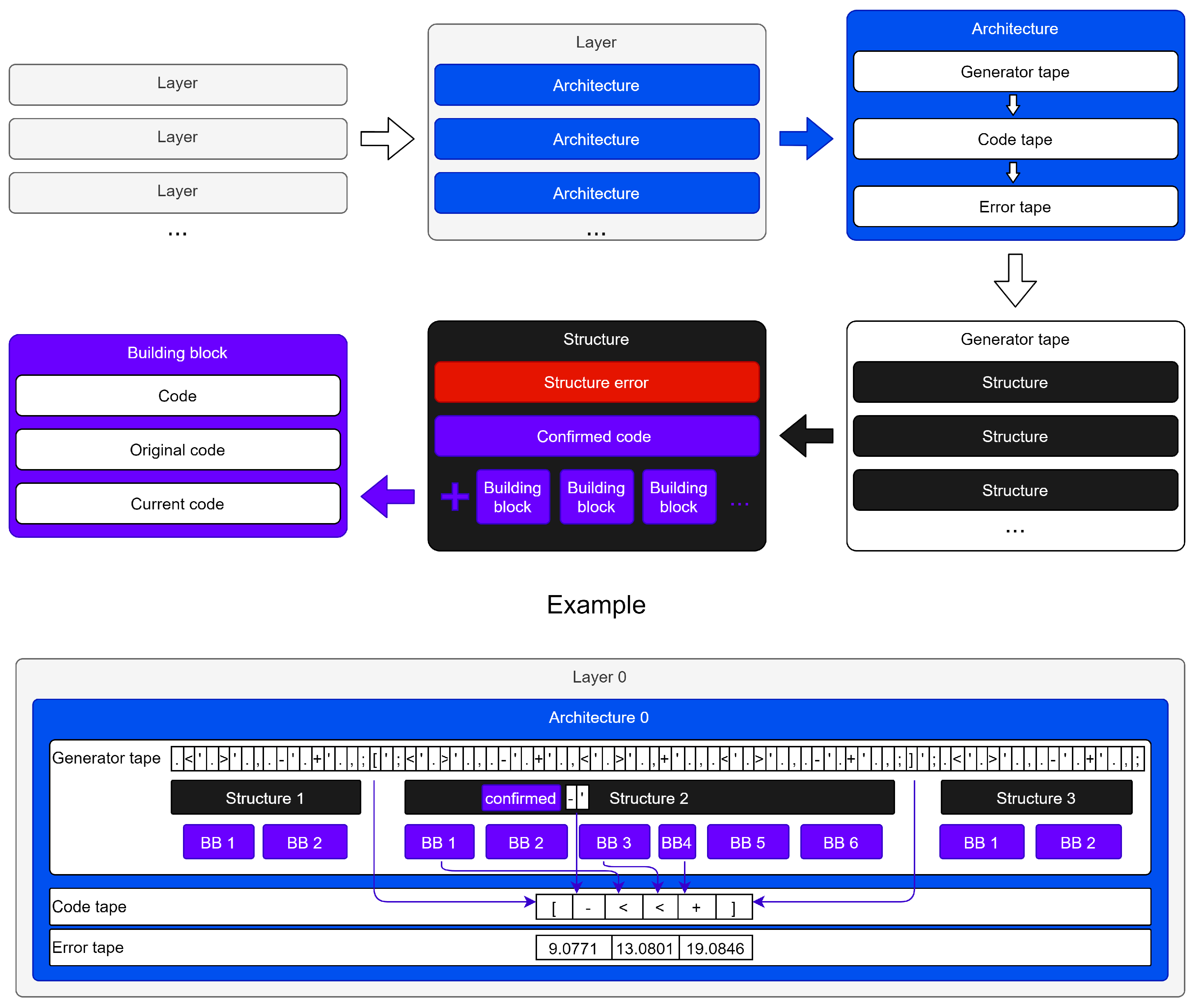
Figure 4.
The generalization problem outside the range of the training values [42]. The authors train an autoencoder to take a scalar value as input, encode the value within its hidden layers, and reconstruct the input value as a linear combination of the last hidden layer. Each autoencoder is identical in its parameterization, tuning, and initialization, differing only in the choice of nonlinearity on hidden layers. For each point in the figure, the authors train 100 models to encode values between −5 and 5 and average their ability to encode values between −20 and 20.

Figure 5.
Neural Arithmetic Logic Units with Bias (NALUB) architecture. The matrices of the parameters , , and of the NALU model proposed in [42] are represented in the lower part of the figure. The matrix (where tanh denotes the hyperbolic tangent function) has all the values within the interval , whilst the matrix (where denotes the sigmoid function) is composed only of values within the interval . Therefore, their elementwise product yields matrices with elements within the interval and polarized towards the stable points . This allows the NALU architecture to make possible some arithmetic operations on the input vector . The introduction of a bias vector (highlighted in red in figure) further extends the set of possible operations. For instance, specific configurations of and enable the NALU model to obtain a component of the output vector as a product of two components of the input vector . The introduction of the bias vector, hence, allows us to multiply, divide, add, and subtract these components with constants. The bias is added after having carried out the matrix product between the matrix and the vector .

Figure 6.
Different plots of the function for , respectively.

Figure 7.
Neural Arithmetic Logic Units with Bias Tetration controlled Cell (NALUBTC) architecture. In the NALU architecture [42], the addition and subtraction operations are obtained by directly multiplying the input vector by the transformation matrix and the resulting vector is . To perform a multiplication or a division, the vector is first transformed by applying the operation to each component. This way, the sum of the logarithms corresponds to the product of the exponents as follows . Therefore, is obtained through the matrix product raised to the exponent. In NALUBTC, we introduce the scalar parameter g (with ), which we use as the height of the tetration function (see Equation (2)). For the value , the possible operations are addition and subtraction, for , multiplication and division, for , exponentiation and root. Hence, the set of possible operations is extended with respect to the NALU architecture, allowing for a more general automated parameter optimization.

Figure 8.
Differentiable Neural Computer (DNC) architecture. The memory is a matrix accessed by content or by address through a reading key. The controller generates the read and write keys. The memory is accessed by the read and write heads, which apply different mechanisms such as attention and gating to determine the extent of the effect of the read/write action on the memory locations. The architecture learns to use memory to represent solutions to the problem. It learns to read and write the data needed to solve the problem. It is able to model, visit, and explore even complex structures, such as networks and graphs, saving the relationships between different inputs in memory. The controller is shown on the left of the figure, along with the input and output of the DNC architecture. The read and write heads are shown on the right of the controller. In the center the memory is represented, the colored lines are the locations accessed. Finally, on the right are represented first the links and then the usage vector, which indicates the locations used recently.
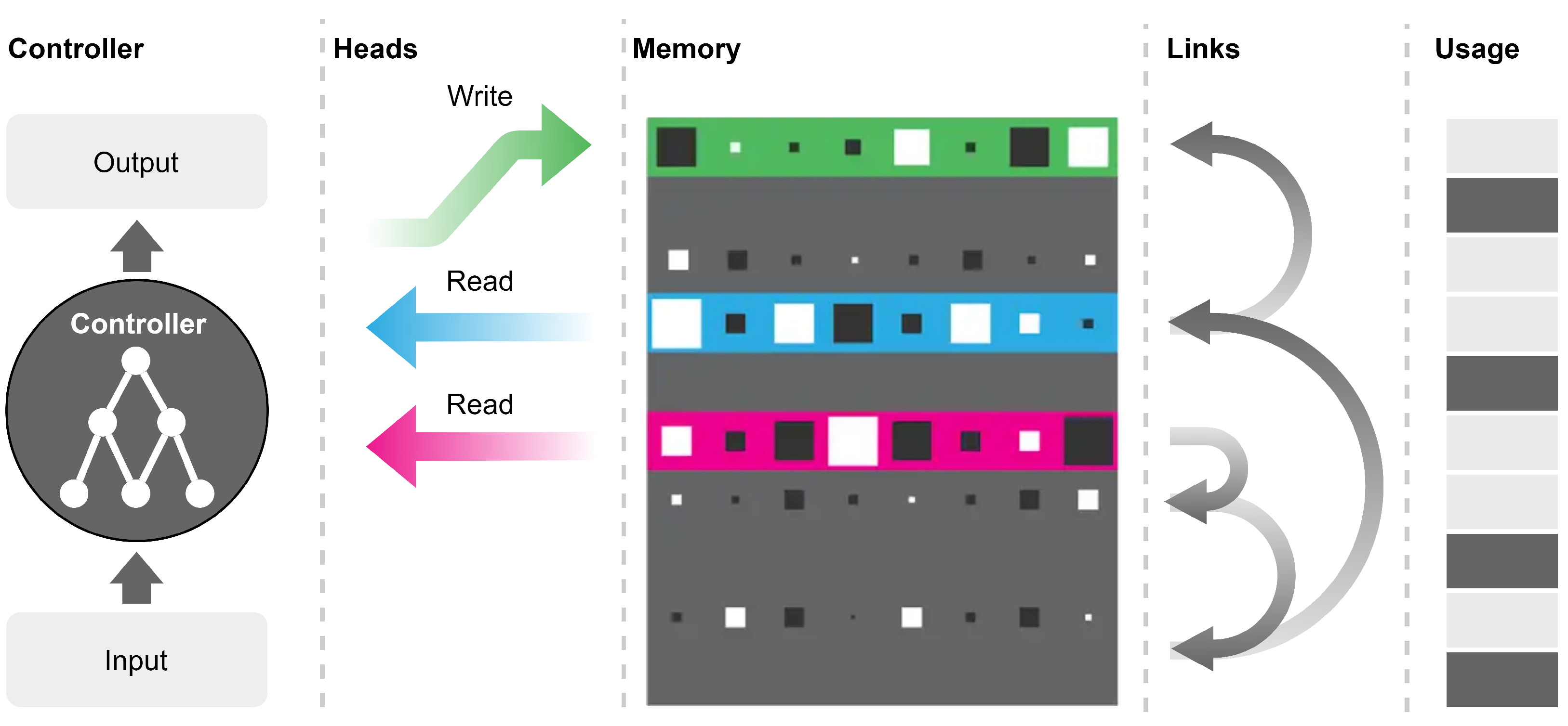
Figure 9.
Differentiable Neural Computer (DNC) grafted model. Compared to the previous figure (i.e., Figure 8) only the controller part has been modified. In the original architecture, the controller is a simple neural network or a recurrent neural network. Differently, in this architecture the controller is itself a DNC.
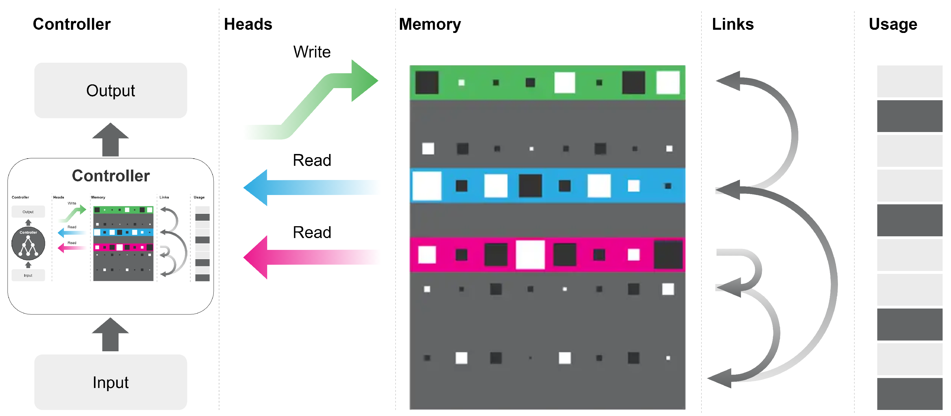
Figure 10.
A diagram showing the high-level functioning of the routing-based Reinforcement Learning architecture implemented on the Deep-Q Network (DQN) model. The first figure on the left shows a frame of the game, cropped and pre-processed. A convolutional network takes the game frame as input and generates the capsules of the first level. Those capsules pass through the capsule network to the final layer: the action capsules. The activated capsule is forwarded to the game environment to select the next action and to the inverse convolutional network. Starting from the activated capsule, the inverse convolutional network reconstructs the prediction of the transaction following the chosen action. The last figure on the right represents a transaction between one frame and the next. The correct figure is obtained by subtracting the game frame reached following an action and the previous frame.

Figure 11.
(a) A graph showing the duration of the experiments in steps for the CartPole-v1 environment during the training for the first experiment on routing applied to Reinforcement Learning. (b) On the top left the current transaction, in the center the prediction of the transition, and on the right the four capsules of the first layer each consisting of four values. The first row displays the current transaction, the second row represents the previous transaction. The numbers above the figure in the last column on the right depend on our choice to adopt the mini-batch normalization as an optimization method. Consequently, the extraction of game frames for training the model occurs randomly. Specifically, the first number (on the left) is the index (assigned randomly) of the transition within the batch. The second number (on the right) denotes the game frame at which the reconstruction is performed. The direction of the arrow connecting the two numbers indicates whether the action chosen by the model is left or right, these being the only two possible actions in the CartPole-v1 game.
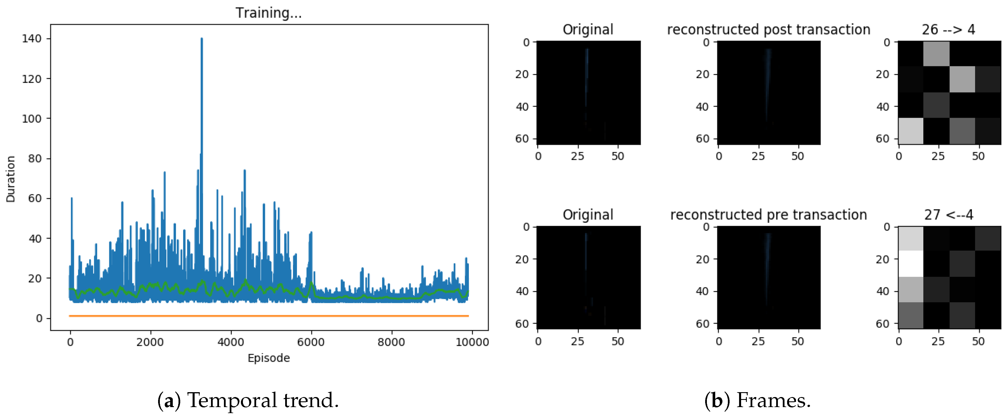
Figure 12.
A different representation for transactions. (b) On the top left the current transaction, in the center the prediction of the transition, and on the right the four capsules of the first layer each consisting of four values. The first row displays the current transaction, the second row represents the previous transaction. The numbers above the figure in the last column on the right depend on our choice to adopt the mini-batch normalization as an optimization method. Consequently, the extraction of game frames for training the model occurs randomly. Specifically, the first number (on the left) is the index (assigned randomly) of the transition within the batch. The second number (on the right) denotes the game frame at which the reconstruction is performed. The direction of the arrow connecting the two numbers indicates whether the action chosen by the model is left or right, these being the only two possible actions in the CartPole-v1 game.

Figure 13.
A diagram showing the high-level functioning of the first Reinforcement Learning architecture with routing implemented on the Advantage Actor-Critic (A2C) algorithm. On the left, a frame of the game with below a four-component vector that encodes the current state of the game. A neural network takes the current state as input and generates the capsules of the first level. Those capsules pass through the capsule network to the final layer: the actor-critic capsules. The A2C algorithm as well as to the inverse convolutional network are applied to the last capsule . Starting from the actor-critic capsule, the inverse convolutional network reconstructs the prediction of the transaction following the chosen action. The transaction is defined as the difference between the vector of the current game state and the previous one.

Figure 14.
A diagram showing the high-level functioning of the second Reinforcement Learning architecture with routing implemented on the Advantage Actor-Critic (A2C) algorithm. This model is similar to the previous one, shown in Figure 13. However, in this case, we have introduced an additional neural network (indicated as Actor in the figure), which returns the chosen action starting from the capsule of the final layer.
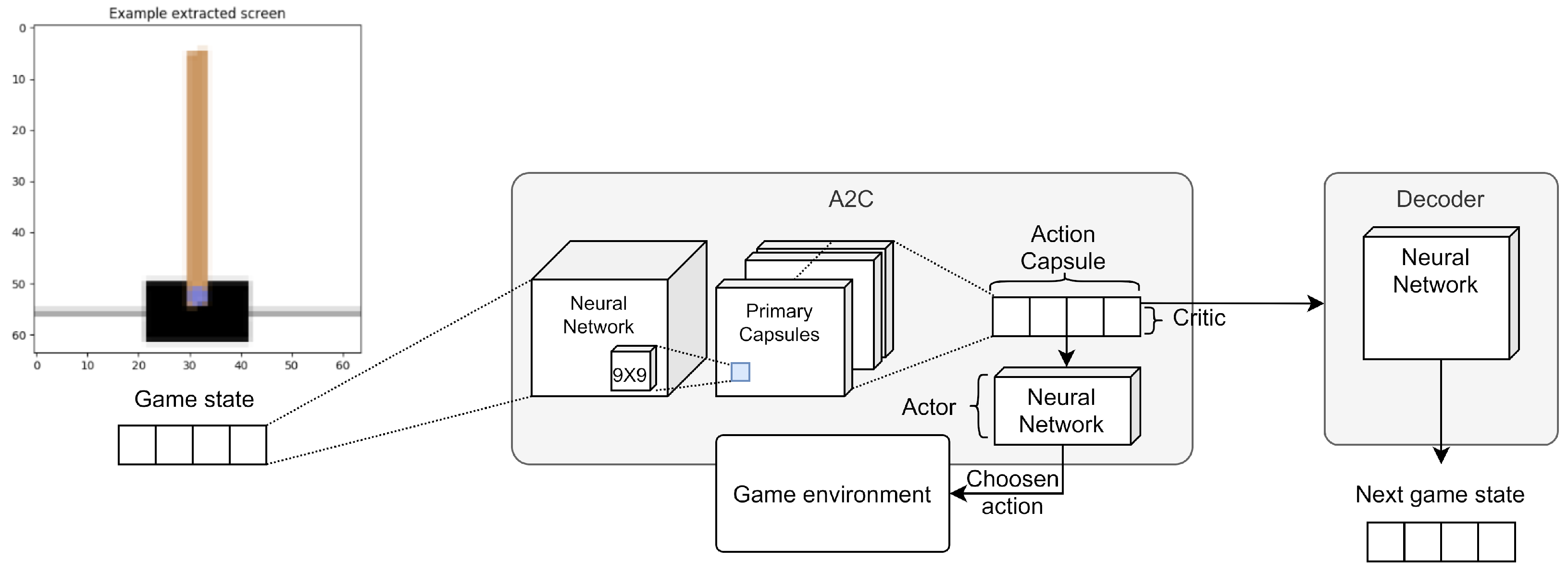
Figure 15.
The experimental path we followed, along with some empirical evaluations of the tested solutions in terms of Interpretability, Efficiency, Structural Invariance, Scale Invariance, and Scalability.
Figure 15.
The experimental path we followed, along with some empirical evaluations of the tested solutions in terms of Interpretability, Efficiency, Structural Invariance, Scale Invariance, and Scalability.
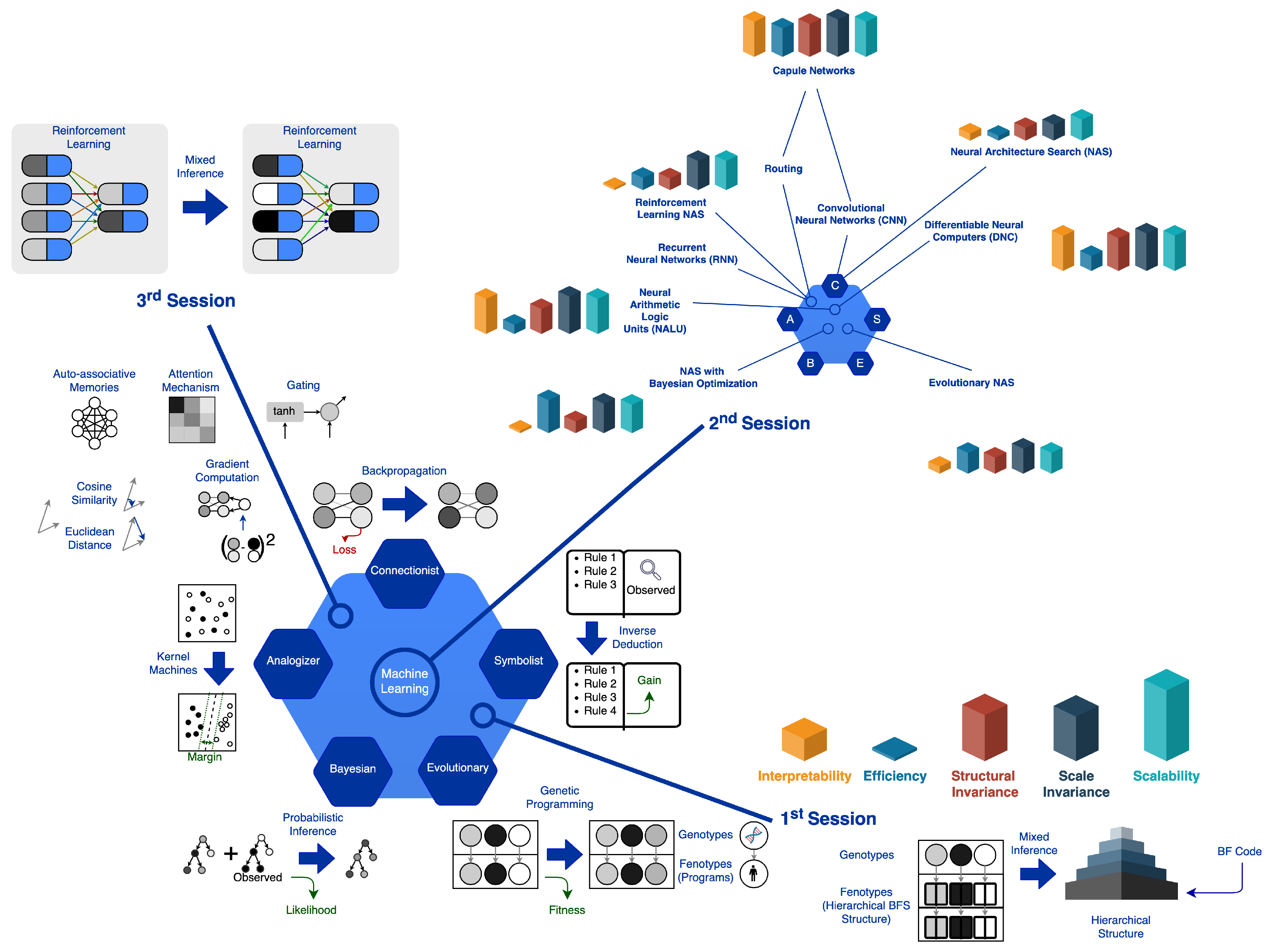

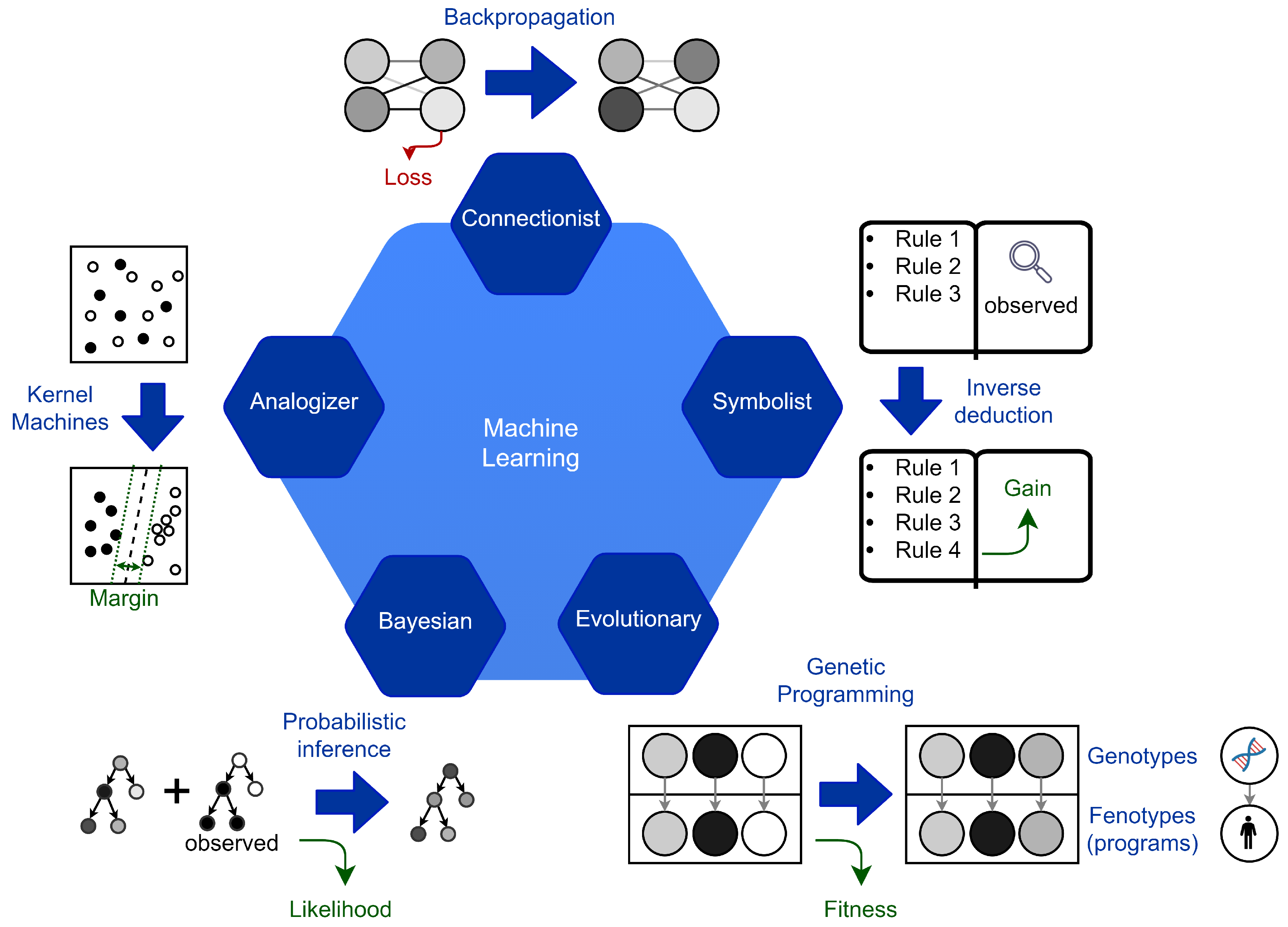
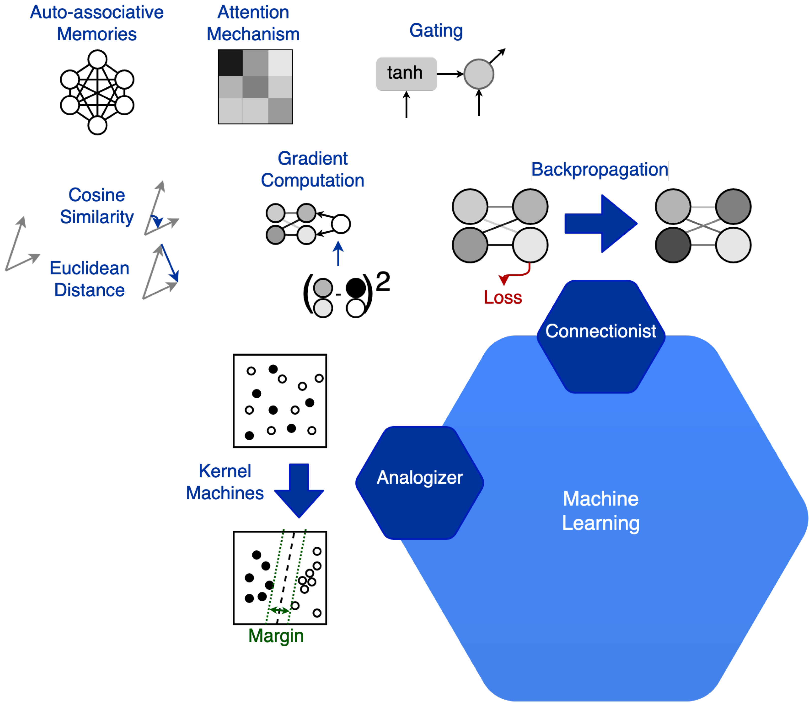
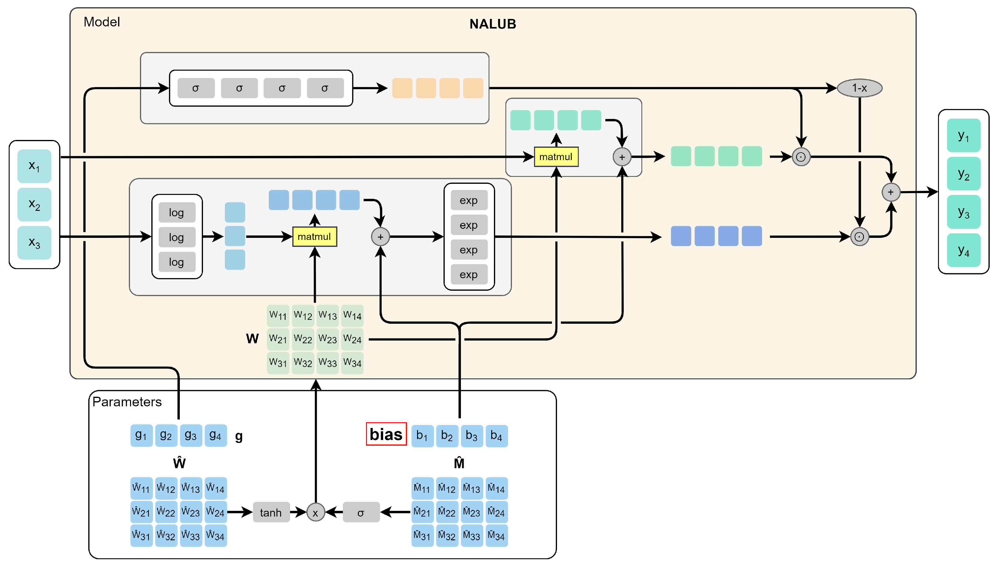
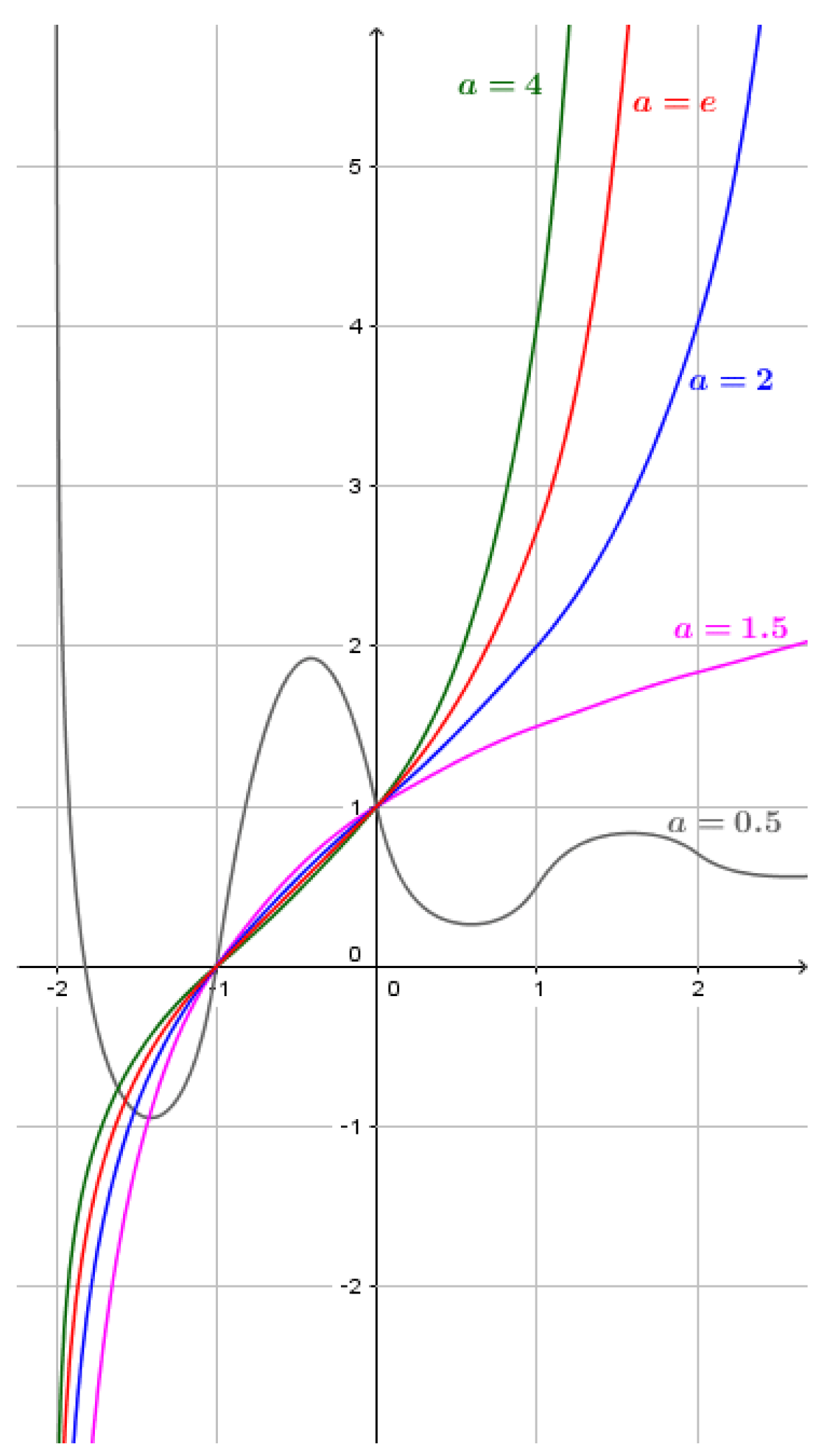
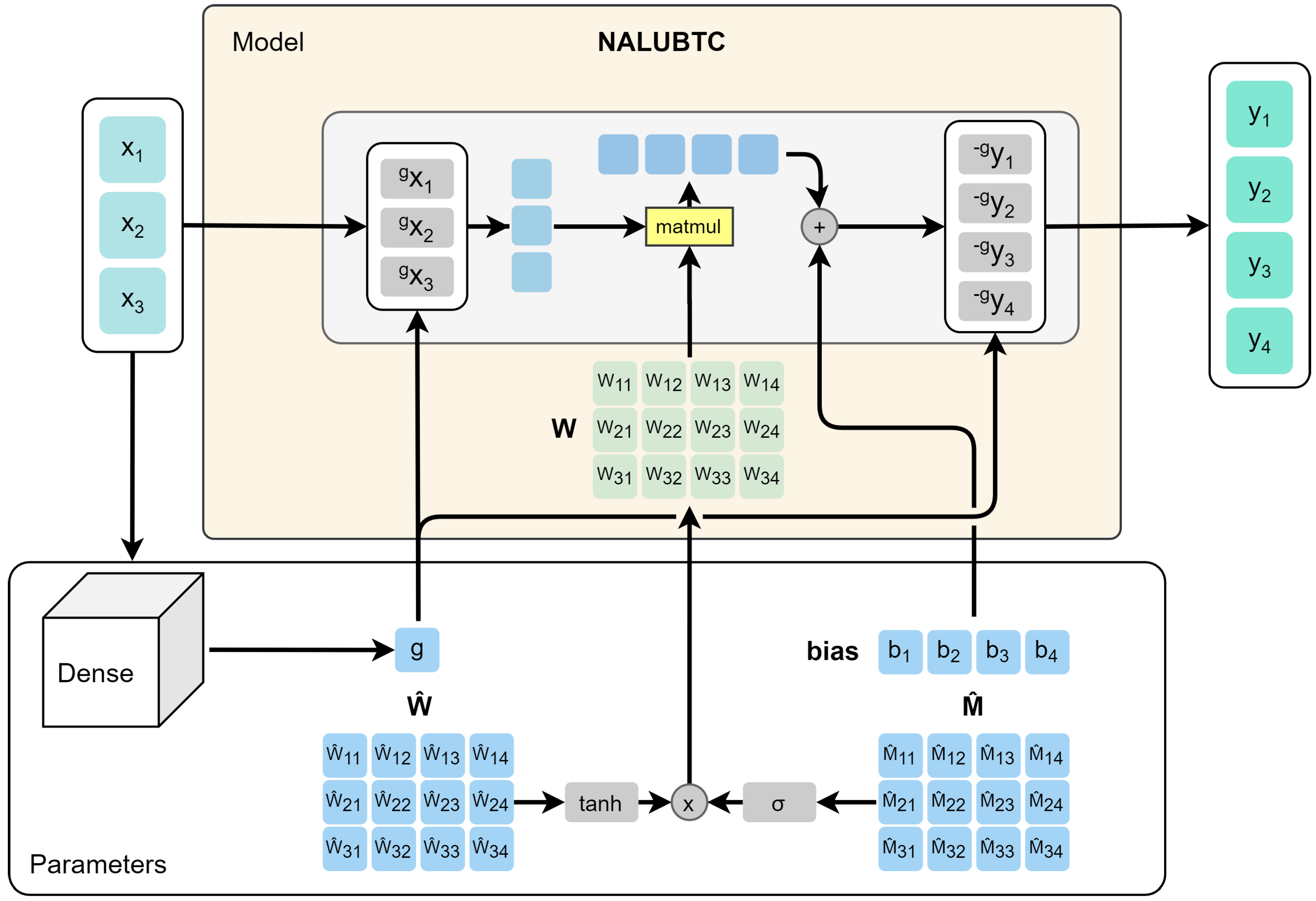
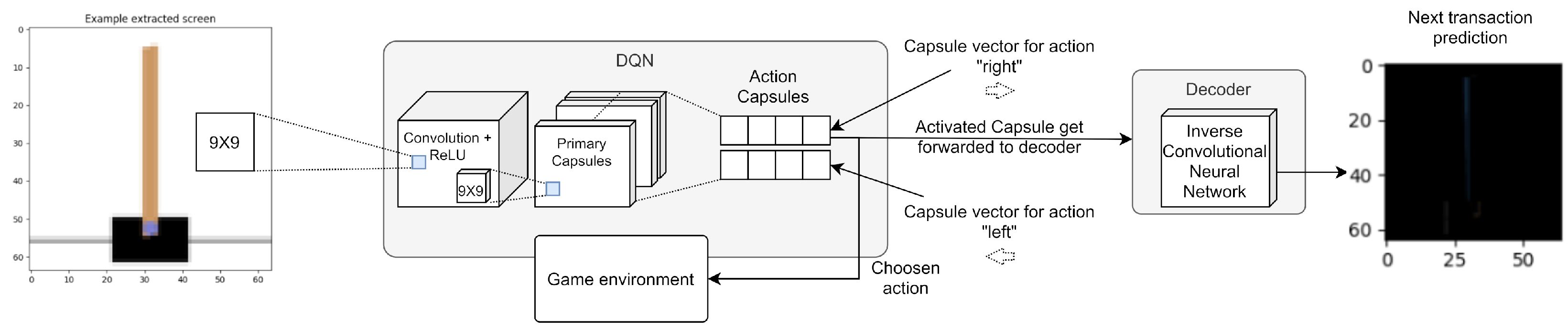
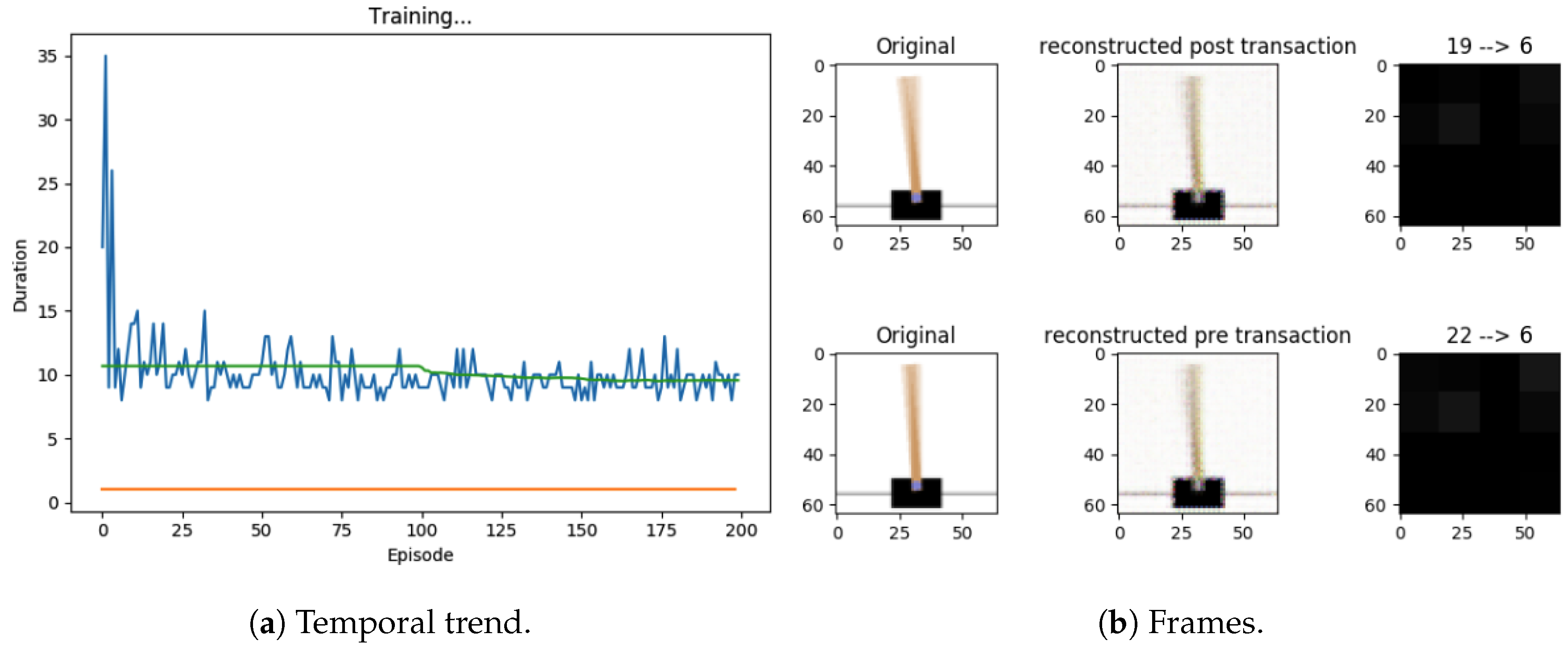
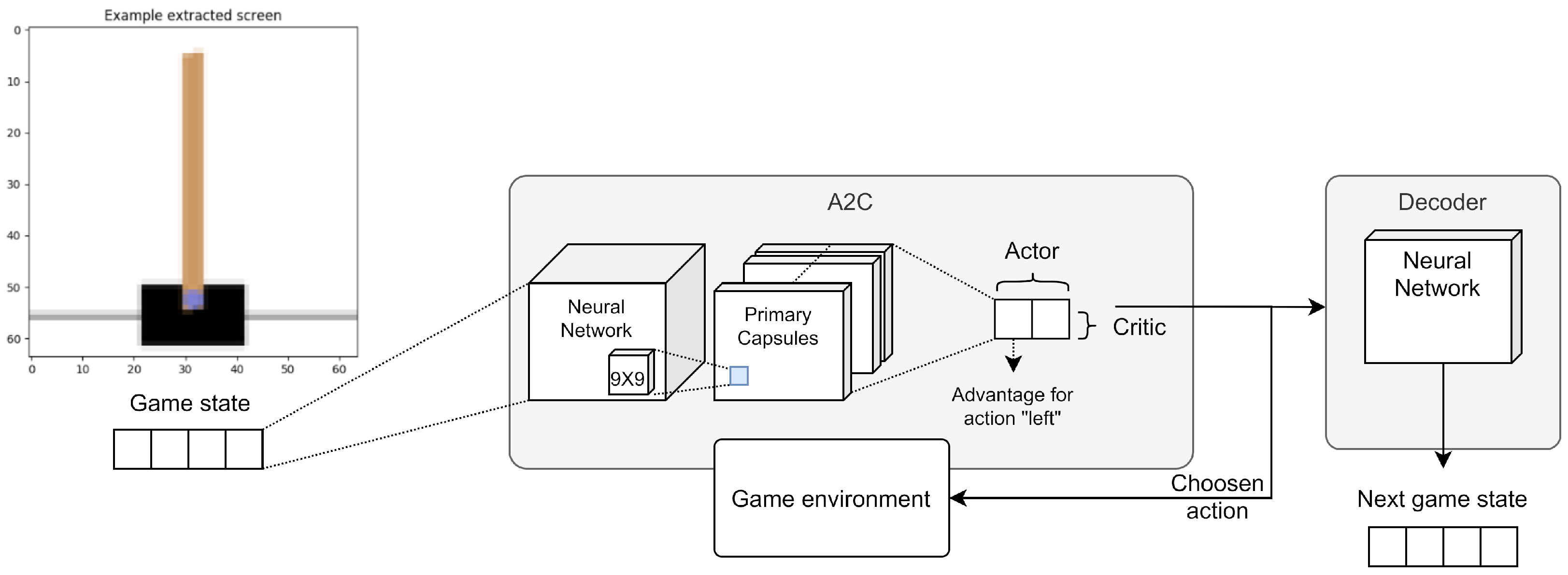
Table 1.
Details of the empirical tests performed on three Atari 2600 games from the Arcade Learning Environment [61].
Table 1.
Details of the empirical tests performed on three Atari 2600 games from the Arcade Learning Environment [61].
| Game | Algorithm | Vision | Capsule Routing | Optimization Algorithm | Learning Rate | Number of Episodes | Solved |
|---|---|---|---|---|---|---|---|
| CartPole-v0 | Actor-Critic (AC) | No | No | Adam | 3.00 | 710 | Yes |
| CartPole-v0 | AC | No | Policy | RAdam | 5.00 | 600 | No |
| CartPole-v0 | AC | No | Policy | RAdam | 5.00 | 600 | No |
| CartPole-v0 | AC | No | Policy | Adam | 5.00 | 600 | No |
| CartPole-v0 | AC | No | Policy | Adam | 1.30 | 1420 | Yes |
| CartPole-v0 | AC | No | Policy | Adam | 2.30 | 1000 | Yes |
| CartPole-v0 | AC | No | Policy | Adam | 2.00 | 710 | Yes |
| CartPole-v0 | AC with corrections | No | Policy | Adam | 2.00 | 710 | Yes |
| CartPole-v0 | AC with memory | No | No | Adam | 3.00 | 1000 | Yes |
| CartPole-v0 | AC with memory | No | No | Adam | 1.30 | 820 | Yes |
| CartPole-v0 | AC | Yes | Vision | RAdam | 5.00 | 1000 | No |
| CartPole-v0 | AC | Yes | Vision | RAdam | 1.30 | 1200 | No |
| CartPole-v0 | AC | Yes | Vision | RAdam | 1.30 | 1000 | No |
| CartPole-v0 | AC without policy | No | No | Adam | 3.00 | 2220 | No |
| CartPole-v0 | AC without policy | No | No | Adam | 3.00 | 1190 | Yes |
| CartPole-v0 | AC without policy | No | No | Adam | 5.00 | 1000 | Yes |
| CartPole-v0 | AC without policy | No | No | Adam | 7.00 | 550 | Yes |
| CartPole-v0 | AC | Yes | No | Adam | 3.00 | 1200 | No |
| CartPole-v0 | AC | Yes | No | RAdam | 5.00 | 3090 | No |
| CartPole-v0 | AC | Yes | No | RAdam | 1.30 | 940 | No |
| CartPole-v0 | AC | Yes | No | RAdam | 5.00 | 1050 | No |
| CartPole-v0 | AC | Yes | No | RAdam | 2.00 | 920 | No |
| CartPole-v0 | AC | Yes | No | RMSProp | 2.00 | 1840 | No |
| CartPole-v0 | AC | Yes | No | RMSProp | 5.00 | 1910 | Yes |
| CartPole-v0 | Deep-Q Network | Yes | Vision+Policy | RAdam | 5.00 | 350 | No |
| CartPole-v0 | Deep-Q Network | Yes | No | RMSProp | 0.01 | 1000 | No |
| CartPole-v0 | Deep-Q Network | Yes | No | RMSProp | 0.01 | 1000 | No |
| CartPole-v0 | Deep-Q Network | Yes | No | RMSProp | 0.01 | 10,000 | No |
| Pong-v0 | AC | Yes | No | Adam | 2.00 | 250 | No |
| MountainCar-v0 | AC | No | No | Adam | 2.00 | 14,000 | No |
Publisher’s Note: MDPI stays neutral with regard to jurisdictional claims in published maps and institutional affiliations. |
© 2021 by the authors. Licensee MDPI, Basel, Switzerland. This article is an open access article distributed under the terms and conditions of the Creative Commons Attribution (CC BY) license (http://creativecommons.org/licenses/by/4.0/).
Share and Cite
MDPI and ACS Style
Vaccaro, L.; Sansonetti, G.; Micarelli, A. An Empirical Review of Automated Machine Learning. Computers 2021, 10, 11. https://0-doi-org.brum.beds.ac.uk/10.3390/computers10010011
AMA Style
Vaccaro L, Sansonetti G, Micarelli A. An Empirical Review of Automated Machine Learning. Computers. 2021; 10(1):11. https://0-doi-org.brum.beds.ac.uk/10.3390/computers10010011
Chicago/Turabian StyleVaccaro, Lorenzo, Giuseppe Sansonetti, and Alessandro Micarelli. 2021. "An Empirical Review of Automated Machine Learning" Computers 10, no. 1: 11. https://0-doi-org.brum.beds.ac.uk/10.3390/computers10010011
Note that from the first issue of 2016, this journal uses article numbers instead of page numbers. See further details here.