Anomalies Detection Using Isolation in Concept-Drifting Data Streams †
by
 ,
,
Maurras Ulbricht Togbe
1,*, 
Yousra Chabchoub
1,
Aliou Boly
2,
Mariam Barry
3,
Raja Chiky
1 and
Maroua Bahri
3 1
ISEP, LISITE, 75006 Paris, France
2
Faculté des Sciences et Techniques (FST)/Département Mathématiques et Informatique, Université Cheikh Anta Diop de Dakar, Dakar-Fann BP 5005, Senegal
3
Télécom Paris, LTCI, Institut Polytechnique de Paris, 91120 Palaiseau, France
*
Author to whom correspondence should be addressed.
†
This paper is an extended version of our paper published in International Conference on Computational Science and Its Applications (ICCSA 2020), Springer.
Computers 2021, 10(1), 13; https://0-doi-org.brum.beds.ac.uk/10.3390/computers10010013
Submission received: 23 December 2020
/
Revised: 9 January 2021
/
Accepted: 12 January 2021
/
Published: 19 January 2021
(This article belongs to the Special Issue Selected Papers from ICCSA 2020)
Abstract
:Detecting anomalies in streaming data is an important issue for many application domains, such as cybersecurity, natural disasters, or bank frauds. Different approaches have been designed in order to detect anomalies: statistics-based, isolation-based, clustering-based, etc. In this paper, we present a structured survey of the existing anomaly detection methods for data streams with a deep view on Isolation Forest (iForest). We first provide an implementation of Isolation Forest Anomalies detection in Stream Data (IForestASD), a variant of iForest for data streams. This implementation is built on top of scikit-multiflow (River), which is an open source machine learning framework for data streams containing a single anomaly detection algorithm in data streams, called Streaming half-space trees. We performed experiments on different real and well known data sets in order to compare the performance of our implementation of IForestASD and half-space trees. Moreover, we extended the IForestASD algorithm to handle drifting data by proposing three algorithms that involve two main well known drift detection methods: ADWIN and KSWIN. ADWIN is an adaptive sliding window algorithm for detecting change in a data stream. KSWIN is a more recent method and it refers to the Kolmogorov–Smirnov Windowing method for concept drift detection. More precisely, we extended KSWIN to be able to deal with n-dimensional data streams. We validated and compared all of the proposed methods on both real and synthetic data sets. In particular, we evaluated the F1-score, the execution time, and the memory consumption. The experiments show that our extensions have lower resource consumption than the original version of IForestASD with a similar or better detection efficiency.
1. Introduction
Data stream mining is a sub-domain of data mining that continuously processes incoming data on the fly. Data stream mining imposes several challenges, such as the evolving nature of data and its huge size, which is potentially infinite. These challenges require efficient and optimized mining methods, in terms of processing time and memory usage, which are adapted to the stream setting. The stream processing must also be performed under the one-pass, aka. single pass, constraint where instances can be accessed a limited number of times (in some cases only once). Multiple applications deal with data streams, such as finance, network monitoring, telecommunications, and sensor networks. The continuous arrival of data streams in rapid, time-varying, and possibly unbounded way may raise new fundamental research problems. As research in the data stream environment keeps progressing, the problem of how to efficiently alert when facing an abnormal behavior, data, or patterns (aka. outliers) still remains a significant challenge to handle. In fact, the outliers should be detected as fast as possible to obtain insights for mining purposes. Stream anomaly detection algorithms refer to the methods that are able to extract enough knowledge from the data in order to compute the anomaly scores while dealing with evolving data streams.
Many solutions have been recently developed for data stream processing that arrive at a single location or at multiple locations. The main idea of these proposed approaches consists in processing data streams on the fly before storing them. In this context, a recent framework has been released for multi-output, multi-label, and data streaming approaches, called scikit-multiflow [1] (see Section 2.2). This framework also includes the popular half-space-trees algorithm [2], a fast anomaly detection for data streams. The principal motivation of the scikit-multiflow developers is to encourage researchers and industrials to easily integrate and share their approaches to the framework and make their work easily accessible by the growing Python community. Therefore, we decided to extend the framework by proposing other anomaly detection approaches that can be applied in the data streams context.
In this paper, we first list the existing frameworks for evolving data streams by highlighting their characteristics. Subsequently, we present the anomaly detection algorithms that have been adapted to the stream setting by discussing the advantages and disadvantages of each of them. Moreover, we present an implementation of some methods that proved to be efficient in the literature within the scikit-multiflow framework. In particular, we implement the isolation-based anomaly detection (IForestASD) algorithm [3] and highlight the simplicity of the framework to ease and accelerate its evolution. Afterwards, we perform different experiments to evaluate the predictive performance and resource consumption (in terms of memory and time) of the IForestASD method and compare it with the well-known state-of-the-art anomaly detection algorithm for data streams, half-space-trees. As far as we know, this is the first open source implementation of this algorithm. Finally, we present some improvements of the methods in order to take the evolution of the stream into account, especially, the appearance of drifts in the data. Because IForestASD does not handle drifts in data, we extend this algorithm by proposing 3 approaches that incorporate efficient drift detection methods (ADWIN and KSWIN, as explained in Section 5) inside the core of the IForestASD algorithm. Therefore, our main contributions are summarized, as follows:
- We survey the anomaly detection methods in data streams with a deep view of the main approaches in the literature.
- We implement the IForestASD algorithm [3]) on top of the scikit-multiflow streaming framework.
The paper is organized, as follows: Section 1 introduces our work and its motivations. Section 2 highlights some background about data stream frameworks and the associated challenges. In Section 3, we provide a survey on anomaly detection for data streams. In Section 4, we discuss isolation-based methods with a focus on the IForestASD algorithm. Section 5 introduces our proposed approaches and how they deal with drifts. We discuss the experimental evaluations of the four implemented methods in Section 6. Finally, Section 7 concludes the work by providing future research directions.
2. Data stream Framework
2.1. Constraints and Synopsis Construction in Data Streams
The evolving nature of data streams raises multiple requirements that need to be addressed by batch algorithms. In this section, we present some principal constraints that are encountered in the stream environment [6,7] that we aim to address in this paper.
- Evolving data: the infinite nature of evolving data streams requires real—or near-real—time processing in order to take the evolution and speed of data into account.
- Memory constraint: since data streams are potentially infinite, therefore, stream algorithms need to work within a limited memory by storing as less as possible of incoming observations as well as statistical information regarding the processed data seen so far.
- Time constraint: stream mining has the virtue of being fast. Accordingly, a stream algorithm needs to process incoming observations in limited time, as fast as they arrive.
- Drifts: concept drift is a phenomenon that occurs when the data stream distribution changes in time. The challenge that is posed by concept drift has been subject to multiple research studies, we direct the reader to a survey on drifts [8].
In order to handle these aforementioned challenges, stream algorithms must use incremental processing strategies to be able to work in a stream fashion. There are several techniques [6,7,9] that can be used in order to address these constraints. We summarize some of them below:
- Single pass: since data stream evolves over time, the stream cannot be examined more that once.
- Windows: window models have been proposed to maintain some of contents the stream in the memory. Different window models exist, such as sliding, landmark, and fading windows [10].
- Synopsis construction: a variety of summarization techniques can be used for synopsis construction in evolving data streams [11], such as sampling methods, histograms, sketching, or dimensionality reduction methods.
2.2. Data Stream Software Packages
Different softwares for data stream mining have been proposed in the literature. In the following, we cite some open-source streaming frameworks with active growing research communities [12].
Massive Online Analysis (MOA) [13] is the most popular open source framework for data stream mining in the research community that was implemented in Java. The MOA software includes a collection of machine learning algorithms (classification, regression, clustering, outlier detection, concept drift detection, and recommender systems) for data stream. Besides, multiple open-source softwares use MOA to perform data stream analytics in their systems [14], including ADAMS, MEKA, and OpenML.
Scikit-multiflow [1] is an open-source framework that is written in Python for multi-label/multi-output and single-label learning for evolving data streams. Scikit-multiflow is inspired by the popular frameworks scikit-learn (https://scikit-learn.org) and MOA.
Similar to the latter, scikit-multiflow also includes a collection of various stream algorithms in different tasks, provides tools for evaluation, and offers the possibility to easily extend algorithms. Given the increasing popularity of the Python programming language, the advantage of scikit-multiflow is that it complements the scikit-learn that is widely used by the data science community, and it mainly focuses on the batch setting. Scikit-multiflow is currently merging with the creme framework, yielding a new python framework for online machine learning in python, named RIVER (https://github.com/online-ml/river), which will be available very soon.
There exist other frameworks for data streams, such as SAMOA [15] and StreamDM (http://huawei-noah.github.io/streamDM/). StreamDM [16] is an open-source framework for online machine learning that is designed on top of Spark Streaming, which an extension of the core Spark API that enables scalable data streams processing. In [17,18], comparative studies of data streams frameworks are presented with a focus on the distributed tools for data stream processing, such as Apache Spark, Storm, Samza, and S4. More frameworks and their details are also provided in [12].
According to the review of big data streams mining frameworks, scikit-multiflow (River) seems to be the most promising one, as it implements the majority of well-known stream learning methods in Python, a programming language with a growing active community. Additionally, since it only contains one anomaly detection method, which is half-space-trees [2], we thus decided to extend this framework by implementing an anomaly detection approach based on Isolation Forest algorithm proposed by Ding and Fei in [3]. Our methods have been implemented using scikit-multiflow as River is not available yet.
Hence, the motivations behind our implementation providing an isolation-based algorithm in scikit-multiflow are the following:
- Isolation Forest is a state-of-the-art algorithm for anomaly detection and the only ensemble method in scikit-learn. It is widely used by the community and it can easily be adapted for online and incremental learning.
- Scikit-multiflow (river) is the main streaming framework in Python, which includes a variety of learning algorithms and streaming methods.
3. Anomaly Detection in Data Streams: Survey
3.1. Existing Methods
Anomaly Detection in Data Stream (ADiDS) presents many challenges due to the characteristics of this type of data. One important issue is that data stream treatment must be performed in a single pass to deal with memory limits and methods have to be used in an online way, as explained in the previous section. Thus, the several existing offline anomaly detection approaches, such as statistical approach, clustering approach, etc., [19,20,21], are not adapted for data stream, because they require many passes over data. They also need to consider the entire dataset to be able to detect anomalies.
Some propositions have been adapted and new designed methods have been performed for ADiDS. The authors of [22] provide a survey on outlier detection methods that can be applied to temporal data with a focus on data streams. They presented evolving prediction models, a distance based approach, and outlier detection in high dimensional data streams. [23,24,25] are all surveys regarding outlier detection in data stream context. In [23], the authors addressed the issues of outlier detection in data stream, like concept drift, uncertainty, and arrival rate.
In the book ([21], Chapter 9), the authors proposed a detailed study of time series and multidimensional streaming outlier detection methods. They presented different approaches, such as probabilistic-based, prediction-based, and distance-based methods.
3.2. Approaches and Methods Classification
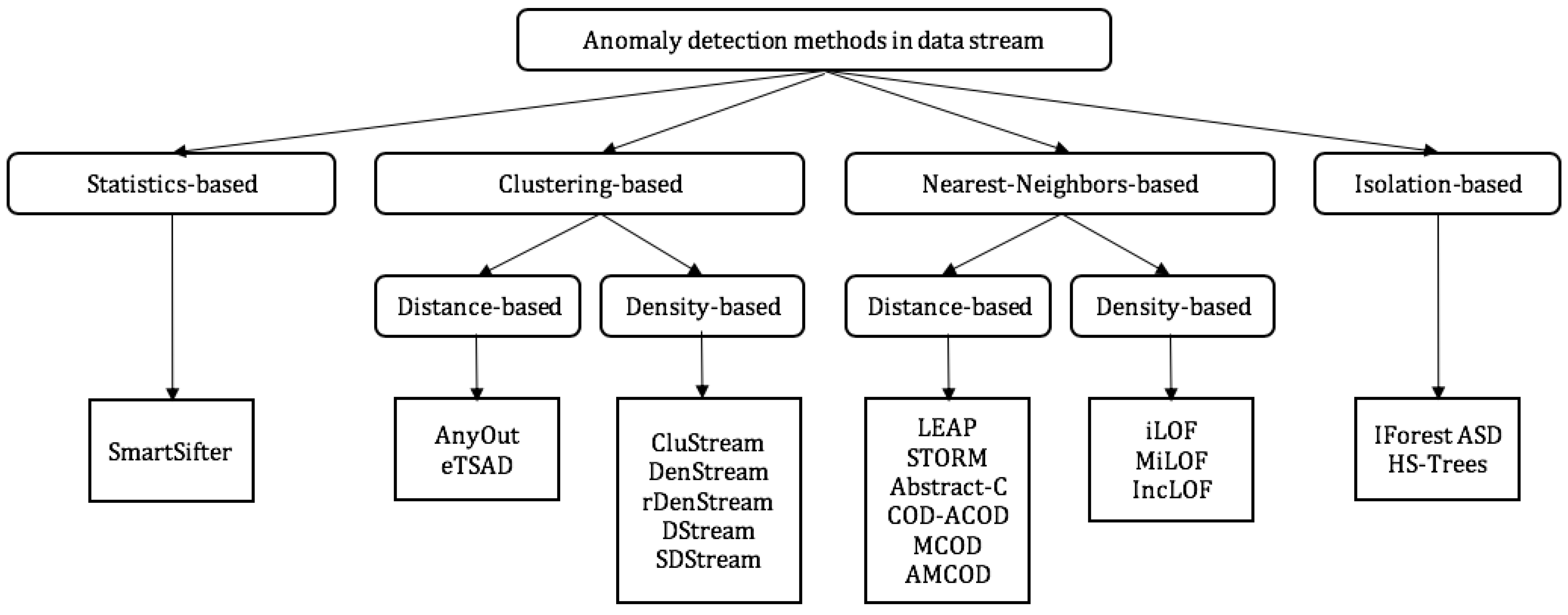
Anomalies are, by definition, rare and they have a different behavior as compared to normal data. These characteristics are correct for static datasets and data streams. In the following, the most used anomalies detection approaches, such as statistics, clustering and, nearest-neighbors, are presented. We will concentrate on an approach that is based on isolation: Isolation Forest, proposed in [26] by Liu et al., as it is the core of our main contributions in this paper.
3.2.1. Statistics-Based
Statistics-based approaches generally define a model that represents the normal behavior that is based on the dataset. Abnormal data are considered to be the new incoming data that do not match the model or have very low probability to correspond the model. In the literature, we find some methods that give a score for the data based on the deviation degree from the model [27].
Statistics-based methods can be parametric, in which case they need to have prior knowledge about the dataset distribution. They can be non-parametric, where they learn from the given dataset in order to obtain the underlying distribution. In the context of data stream, such prior knowledge is not always available.
3.2.2. Clustering-Based and Nearest-Neighbors-Based
Clustering and nearest neighbors approaches are techniques based on the proximity between observations. The methods in these categories are based either on the distance (distance-based) or the density (density-based). Clustering methods split the dataset in different clusters following the similarity between the data. The most distant cluster or the cluster, which has the smallest density, can be considered as an anomaly cluster ([28,29]).
Nearest-neighbors methods determine the neighbors of one observation by calculating the distance between all of the observations in the dataset. An anomaly is considered to be the observation, which is far from its k nearest-neighbors [30]. It is also characterized as the observation that has the most less neighbors in a radius r (a fixed parameter) [31]. These approaches can suffer of a high memory consumption and execution time or a lack of information, since they require computing the distance or density between all of the observations in the dataset or they require having some prior knowledge regarding the dataset.
3.2.3. Isolation-Based
In [26], thw authors present the isolation-based approach, whose principle is to isolate abnormal observations from the dataset. Anomalies data are considered to be very different when compared to normal data. They are also supposed to represent a very small proportion of the whole dataset. Thus, they are likely to be rapidly isolated. In Section 4, some of the isolation-based methods are exposed.
Isolation based methods are different when compared to others statistics, clustering, or nearest-neighbors approaches. They have a lower complexity, are more scalable, and do not suffer from the problem of CPU, memory, or time consumption, since they do not calculate a distance or density from the dataset. Thus, isolation based methods are adapted to the data stream context.
Table 1 summarizes advantages and disadvantages of the existing approaches for ADiDS.
In the literature, several works have been performed for adapting or designing for ADiDS. They generally use the data stream concept of window in order to determine anomaly [25]. Figure 1 presents some anomaly detection methods of these approaches.
A recent work [32] on anomaly detection approaches has shown that the isolation forest algorithm has good performance when compared to other methods. Thus, we decided to implement an adaptation of isolation forest in a data stream mining framework. In the following sections, we will describe our contributions that are based on this algorithm.
4. Isolation Forest, IForestASD and HSTrees Methods
Liu et al. proposed the original version of isolation Forest IForest in 2008 [26,33]. This version addressed static datasets. In 2013, Ding and Fei designed an adaptation of IForest to data stream context while using sliding windows [3]: Isolation Forest Algorithm for Stream Data (IForestASD).
There are many other improvements and extensions of Isolation Forest. As an example, Extended Isolation Forest (EIF) [34] addressed a particular weakness in IForest that is caused by the successive splits according to the randomly chosen dimension. In fact, this splitting method engenders some fictitious zones with inconsistent scores, which gives classification errors. The key idea of EIF is to split data according to a randomly chosen hyper-plan that is generated from data dimensions. Functional Isolation Forest [35] is the adaptation of IForest to functional data. Liu et al. have proposed the SCiForest method [36] to detect local anomalies. Marteau et al. proposed an improvement of IForest, named Hybrid IForest, in order to make IForest able to detect anomalies in various datasets with different distributions [37].
In another context, in [38], the authors recently proposed an adaptation of IForest for categorical and missing data. Entropy IForest (E-IForest) method has been proposed in [39] for the choice of the optimal dimension to split a node. In [40], Zhang et al. proposed LSHIForest (Locality-Sensitive Hashing IForest) to generalize IForest to other measures of distance and data spaces. Simulated Annealing IForest (SA-IForest) [41] is an improvement of IForest, which aims to create a more generic forest in the training phase.
Recently, Bandaragoda et al. proposed isolation while using the Nearest Neighbor Ensemble (iNNE) [42] method to overcome some weaknesses of IForest when detecting local anomalies, anomalies with a high percentage of irrelevant attributes, anomalies that are masked by axis-parallel clusters, and anomalies in multi-modal datasets.
All of those adaptations and improvements cited above are designed for static datasets and they are not adapted for data streams.
A detailed description of IForest and IForestASD is given in the following sections.
4.1. Isolation Forest Method
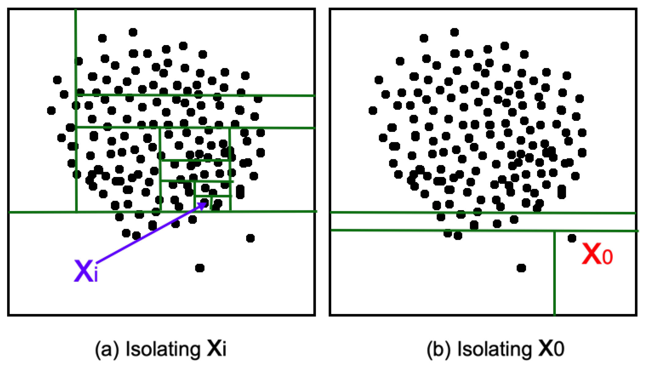
Isolation Forest uses successive data splits to isolate anomalies. It is based on the following two characteristics of anomalies: first, anomalies are supposed to be the exception: they represent a very small proportion of the whole dataset. Second, they have a different behavior when compared to the normal data. With those properties, a relatively small number of partitions is needed in order to isolate anomalies, as shown in Figure 2.
IForest is based on a forest of random distinct itrees. Every tree has to decide whether a considered observation is an anomaly or not. If a random forest of itrees globally considers an observation as an anomaly, then it is very likely to represent an anomaly.
IForest is composed of two phases: the first one is the training phase, which is the construction of the forest of random itrees, and the second one is the scoring phase, where IForest gives an anomaly score for every observation in the dataset.
In the training phase, all of the t random and independent itrees of the forest are built. Using the sample of randomly selected data, every internal node of the binary itree is split in two other nodes (left and right). In order to split one node, IForest randomly chooses one attribute: d from the m data attributes. Subsequently, it randomly chooses a split value v between the min and the max value of d in the considered node. IForest splits internal nodes until a complete data isolation or reaching a maximal tree depth, called , which is equal to .
After the forest training phase, the scoring phase can begin. In this phase, every new observation x has to pass through all of the t itrees to obtain its path length [26]. The anomaly score of x is computed with this formula:
where is the average path length of x over t itrees and is the average path length of unsuccessful search in Binary Search Tree (BST). with ( is Euler’s constant). Finally, if is close to 1, then x is considered as an anomaly. If is less than , x is considered as normal data.
4.2. IForestASD: Isolation Forest Algorithm for Stream Data Method
Isolation Forest is an efficient method for anomaly detection with relatively low complexity, CPU, and time cosunmption. It requires all of the data in the beginning to build t random samples. It also needs many passes over the dataset to build all the random forest. Accordingly, it is not adapted to the data stream context. In [3], the authors have proposed the so-called IForestASD method, which is an improvement of IForest for ADiDS. IForestASD uses sliding window to deal with streaming data. On the current complete window, IForestASD executes the standard IForest method to obtain the random forest. This is the IForest detector model for IForestASD.
IForestASD method can also deal with concept drift in the data stream by maintaining one input desired anomaly rate (u). If the anomaly rate in the considered window is upper than u, then a concept drift occurred, so IForestASD deletes its current IForest detector and builds another one while using all of the data in the considered window.
4.3. Streaming Half-Space Trees
Streaming half-space trees (we will denote by HSTrees) is an online anomaly detection algorithm that is proposed by Tan et al. [2], which deals with streams. This method uses an unsupervised learning approach that can learn patterns from data-streams with continuous numerical attributes where the number of features is constant.
The principle of the algorithm consists of splitting the features space into an ensemble of sub-spaces using a binary trees (called half-space trees ) to build the ensemble. Each node of the trees has a splitting attribute chosen randomly and represents a given work-space (range of values for a given features) and the two children nodes refer to two sub-spaces representing, respectively, the half-space of the parent node space.
Thus, any data point in the domain can traverse a unique path from the root of a HST to one of its leaves, traversing all of the nodes where the data point is contained. The anomaly score of half-space trees relies on Mass profile computation, which refers to the number or points or instance observed in a given half-space. The lower the mass, the higher the anomaly probability.
The data-stream is then also partitioned into short windows of a set length of data points. At any given time, we only consider two consecutive windows, the current one, called latest window, and the preceding one, which is referred to as the reference window. Once the data points have been recorded in a latest window, it is considered to be full, and it becomes the reference window. When the next data point arrives, a new latest window begins. A data stream’s content is used in order to compute and update the mass profile of each node traversed by the instances in the stream, where each node has two counters, r for the reference mass profile and l for the latest mass profile.
One key advantage of the algorithm is that the training phase has constant amortized time complexity and constant memory requirement. When compared with a state-of-the-art method (Hoeffding Trees), it performs favorably in terms of detection accuracy and run-time performance.
4.4. Main Differences between HSTrees and IForestASD
HSTrees and IForestASD have been proposed in order to detect the anomalies in data flows; they are different on several points: training, testing, and model updating phases.
- The training phase: before the trees are built, while IForestASD chooses from the original dataset a sample of data without replacement for each tree planned for the forest, HSTrees creates a fictitious data space. Indeed, for each dimension of the original dataset, HSTrees creates a minimum and maximum value:being a random value in .IForestASD needs a sample of the original dataset to build the ensemble, while HSTrees can build trees structures without any data. During the construction of the trees, to split a node, while IForest ASD chooses a random split value v between and , for HSTrees v is the average of the (fictitious) values of the node, . Note that the maximum size of a tree () with IForestASD is a function of the sample size () while it is a user-defined parameter for HSTrees. Accordingly, to build the trees in the forest, HSTrees has no knowledge of what dataset to use, except the number of attributes. While IForestASD is closely dependent of the dataset.
- Score’s computation: to calculate the score of a given data, IForestASD is based on the length of the path of this data in each tree (as described in Section 4.1) then HSTrees is based on the score of the data for each tree. The overall score of the data is therefore for IForestASD based on the average of the path covered in all the trees in the forest, whereas it will be a sum of the scores that were obtained at the level of each tree in the forest for HSTrees. Unlike IForestASD, which normalizes the average length with when calculating the score, HSTrees limits the number of instances that a node can have in a tree, i.e., sizeLimit. This is a parameter that is predefined by the user.
- Drift Handling approach: the concept drift consists of the normal change of the values of the observations. Both of the methods update the base model (the forest) in order to handle the concept drift. However, while IForestASD updates its model on the condition that the anomaly rate in a window is greater than the preset u parameter, HSTrees automatically updates its model for each new incoming window.
- Model Updates policies: HSTrees updates the model after the completion of each batch by resetting, to 0, the mass value of each node in each tree. However, IForestASD updates the model when the rate of anomalies in the window is greater than a predefined parameter u by retraining a new Isolation Forest model on the last window.
To recap, although IForestASD and HSTrees are both based on the principle of isolation, they have many major differences. In order to compare the performance of these two anomalies detection methods, we carried out, in the following sections, several comparative experiments on different datasets.
5. Drift Detection Methods
IForest ASD [3] (also called IFA in the rest of the paper) is an adaptation of IForest to data stream by simply adding a windowing approach (applying IForest to a window of data). The authors have also added a drift detection phase. Because the stream is evolving, the underlying distribution may change over time. Therefore, the current learned model may be no more representative for the next incoming instances which can impact the quality of learning. In order to cope with this issue, stream algorithms are generally coupled with a drift detection mechanism in order to deal with the new trends as soon as they appear. More details about concept drifts are given by Gama et al. in this survey [8].
In order to detect the concept drift, IForestASD maintains a u parameter that corresponds to the rate of anomalies that should not to be exceeded in the windows. This parameter is given as an input to the algorithm. Thus, if, in a window, the rate of anomalies detected by the model is greater than u, then IForestASD updates its model with the data in the current window, while assuming that data drift has occurred. Two scenarios are possible: the user gives a u lower than the reality, in which case the model will be updated in each window. The second possibility is to give a u higher than the reality which implies that the model will never be updated since drift will never be detect even if it occurred. Thus, u should be correctly defined in order to detect the drift in the data stream. In an unsupervised mode where there is no information or knowledge about the data, providing a u parameter becomes problematic, and IForestASD’s ability to detect drift depends on it. Therefore, in this extended version, we propose improving IForestASD by proposing two approaches based on a drift detection that can be done at two levels: model drift detection ADWIN (ADaptive WINdowing) or data drift detection KSWIN (Kosmolgorov Simirnov WINdows).
5.1. ADWIN for IFA
Several change detection methods have been proposed in the literature [8]. For instance, ADWIN [43], which is a well-known change detector and estimator that consists in maintaining a variable-length window W that keeps the most recent instances of the stream with the constraint that the window has the maximal length statistically consistent with the hypothesis "there has been no change in the average value inside the window" [43]. Technically, ADWIN compares the mean difference of any two sub-windows, of old instances and of recent instances, from W. If the difference is statistically significant, then ADWIN erases all of the instances from , which represent an old concept, and keeps forward.
In the following, we aim to use ADWIN, in a first attempt, to detect changes in the distribution thanks to its strong theoretical guarantees and its capabilities in detecting drifts that have been proved in a wide range of stream algorithms, such as adaptive Hoeffding trees [4] and ensembles [44].
ADWIN provides two methods for detecting drift. First, every instance is added to ADWIN while using the add _element() function. This function takes a one dimensional numeric value (int or float) and adds it into the adaptive window. The second function is detected_change(). It computes the drift detection that is explained above in the current adaptive window and returns a boolean value that informed whether the drift was detected or not. The reader can refer to [1,43] for more information regarding the implementation of ADWIN.
In the IForest model, two results are returned: the data score and the prediction of the model (0 or 1), both can be used as input values for ADWIN. Figure 4 presents our proposed ADWIN based improvements of IForestASD for drift detection. The drift detection phase is managed by ADWIN. Two improvements have been proposed: one based on the model prediction, called PADWIN IFA (Section 5.1.1), and the other one based on the data score that is given by the model, named SADWIN IFA (Section 5.1.2).
5.1.1. PADWIN IFA
The idea behind this improvement is that, in the case of data drift, the prediction will also drift. That is why we decide to use the prediction that is given by IForest as input to ADWIN. In the PADWIN IFA version, the drift detection is based on the predictions of the model (1 or 0) that are given to the add_element() function. If ADWIN detects the drift, we update the model. Otherwise, we handle the following windows while using the existing model.
5.1.2. SADWIN IFA
The prediction of IForest is based on a score computed for each data. Thus, the score is more representative of actual data than its predictive class, since the prediction is dependant on a predefined threshold. Therefore, we propose using the score as input to the add_element() function of ADWIN and call this new version SADWIN IFA. If ADWIN detects the drift, then we update the model; otherwise, we handle the following windows while using the current IForest model.
As explained above, all of the ADWIN based improvements detect the drift of the model after the computation of anomalies detection. This means that the previous window is lost, because all of the predictions are probably false. To solve this problem, we propose another improvement that detects the drift and updates the model before detecting the anomalies. Because ADWIN is designed for assessing a model quality, it cannot be directly applied on raw data. Recently, a new data drift detection method, called Kolmogorov–Smirnov WINdowing (KSWIN) [5], has been proposed in the literature and has been implemented in the scikit-multiflow framework.
5.2. KSWIN for IForestASD
KSWIN and NDKSWIN IForestASD
KSWIN [5] is a recent method for concept drift detection that is based on the well-known Kolmogorov–Smirnov (KS) statistic test [45,46]. The KS-Test is a non-parametric test that does not need any assumption of the underlying data distribution. KS-Test is able to handle only one-dimensional data. It compares the absolute between two empirical cumulative distributions.
Similar to ADWIN, KSWIN also implements the two functions: add_element() to add the new one dimensional data in the local sliding window . The second function is detected_change(), which informs whether the drift is detected or not. has a fixed size. Thus, before adding any new data in , the old data are removed and the new one are added at the queue of the sliding window. Figure 5 describes this process.
Because the KS-Test needs two windows to compute the distance, in KSWIN, authors divide the local sliding window into two parts. The first one R contains the predefined parameter r newest arrived data: . The second window W samples data by uniformly selecting data from the old data in . The uniform distribution used is:
Thus,
The concept drift is detected in KSWIN when , where is the probability for the statistic of the KS-Test.
The KS-Test is a one dimensional method. However, data streams can be multidimensional, thus it is important to adapt KSWIN for this context. For this purpose, we propose a N-Dimensional KSWIN (that we call NDKSWIN in the rest of the paper). The idea of NDKSWIN is to declare a drift if a change is detected for at least one of the n dimensions (while using KSWIN).
Figure 6 shows the workflow of using NDKSWIN as an improvement for IForestASD in order to detect drift before anomalies. A first window is used to create the NDKSWIN instance with all of the needed parameters. It is also used to compute the anomaly detection model while using IForest approach. For the following windows, before applying the anomaly detection, all of the windows must pass through NDKSWIN Step. The add_element() function randomly chooses n samples from the window and randomly selects n dimensions. For every selected data, each value for every selected dimension must pass the KSWIN detected_change() test. If change is detected, the model is updated with all of the data in the current window. No matter the result of the NDKSWIN, the current window must pass through the IForest model for anomaly detection.
6. Experimental Evaluation
This section aims to discuss experiments results to support our two contributions: first, the implementation of IForestASD algorithm in a streaming framework and, secondly, the improvement of this algorithm by incorporating relevant drift detection methods. The section will be organized, as follows:
- explain the experiments set up and material used to reproduce the work;
- provide the results of our implementation with a deep comparison with half-space trees; and,
- compare of the novel proposed algorithms and their performance related to the original version.
6.1. Datasets and Evaluation Metrics
6.1.1. Datasets Description
We tested the different methods discussed above on three well known real datasets [47], which have been used in the original paper of IForestASD.
We also used a simulated stream data with different configurations to compare IForestASD to our proposed improvements. We performed a benchmark with the half-space trees method on a variety of configurations (12 for each dataset). We generate the simulated stream while using the SEAGenerator that is available on scikit-multiflow, which is based on the proposed data stream generator in [48]. As described in the scikit-multiflow documentation, (https://github.com/scikit-multiflow/scikit-multiflow/blob/master/src/skmultiflow/data/sea_generator.py), “It generates 3 numerical attributes, that vary from 0 to 10, where only 2 of them are relevant to the classification task. A classification function is chosen, among four possible ones. These functions compare the sum of the two relevant attributes with a threshold value, which is unique for each of the classification functions. Depending on the comparison, the generator will classify an instance as one of the two possible labels”. These stream data, called SEA, have noise but do not have any drift. Thus, we expect that the experimented methods do not detect any drift. Table 2 summarizes the characteristics of the datasets.
6.1.2. Experimental Setup
In order to compare HSTrees and IForestASD in one hand and compare IForestASD to SADWIN IFA, PADWIN IFA, and NDKSWIN IFA in other hand, we performed experiments while using the hyper-parameters that are described in Table 2.
The number of observations (samples) is 10,000 for both datasets in each experiment. The anomaly threshold is set to . We set the value of the parameter u to the real anomalies rate in the datasets, as proceeded for IForestASD in [3]. This value is used in order to detect drift and reset the anomaly detection model as shown in Figure 3.
According to the results that were obtained in Table 3, with 30 itrees, IForestASD gives good performances. Regarding the window size, the performances decrease after 500. Accordingly, we use and for the comparison between IForestASD IFA, SADWIN IFA, PADWIN IFA, and NDKSWIN IFA.
6.1.3. Evaluation Metrics
We addressed the following three metrics: F1 score, Running Time (training + testing) ratio (IForestASD/HSTrees), and Model Size ratio (HSTrees/IForestASD) for the implementation of IforestASD.
The performance of the models is measured following the prequential (test-then-train method) evaluation strategy that is specifically designed for stream settings, in the sense that each sample serves two purposes (test then train), and that samples are analyzed sequentially, in the order of arrival, and become immediately inaccessible. This approach assures that the model is tested on new samples that have not been used in the training yet. All of the metrics have been provided by the framework scikit-multiflow while using the prequential evaluator (https://scikit-multiflow.github.io/scikit-multiflow/documentation.html).
6.1.4. F1 Metric
It corresponds to the harmonic mean of precision and recall, and it is computed, as follows:
F1 is a useful metric in case of imbalanced class distribution. This is the case of abnormal data that are less represented than normal data.
6.1.5. Model Size Ratio (HSTrees Coefficient Ratio)—HRa
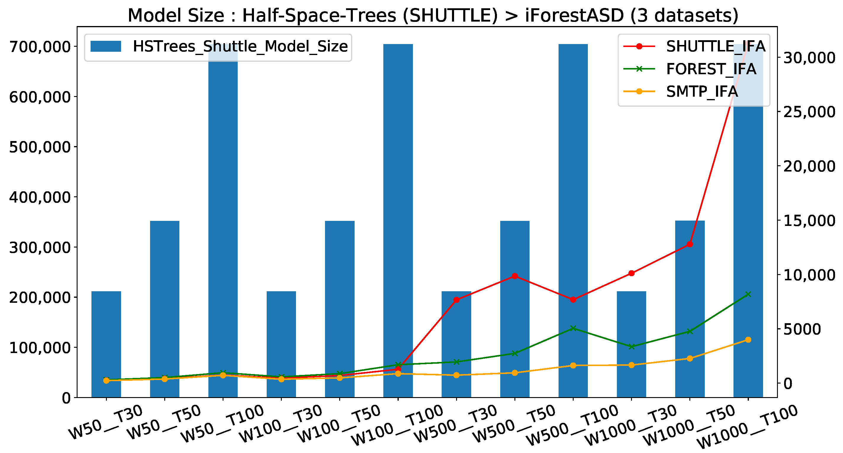
In the opposite of the running time, when we consider the model size, we observe that IFA always used less memory than HST. Hence, to compare these two methods, we compute the ratio of the higher value (HST) over the smaller value (IFA) to obtain the HST coefficient. Figure 7 reports the impact of parameters choice on resources used (model size absolute value in Kilo-bytes) for both HSTrees and the evolution of resources used for the three datasets when window size and number of trees vary. Interpretations are provided below.
6.1.6. Running Time Ratio (IForestASD Coefficient Ratio)—IRa
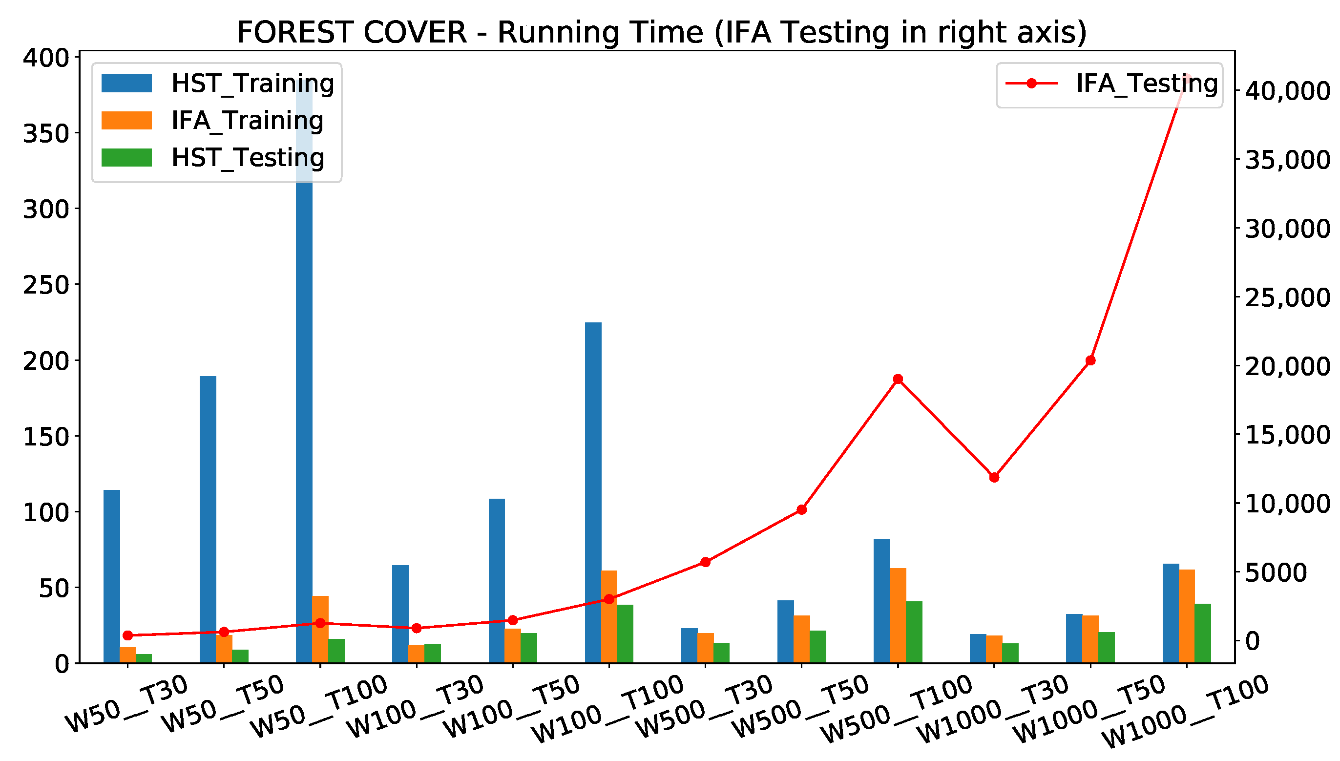
Because half-space trees (HST) is always faster than IForestASD (IFA), for both training and testing time, by an order of 400 for the worst case, we reported the ratio between running time (training and testing) of the two models: IFA over HST. For example, for the Forest-Cover data, IFA is three times slower than HST for , and for the running time ratio is 391 in the Table 3, which means that IFA is 391 slower than HST. The absolute values of running time (in seconds) and their evolution over hyper-parameters variation are reported in Figure 8.
The source code of the different experiments can be found in the Github at https://github.com/Elmecio/IForestASD_based_methods_in_scikit_Multiflow.
6.2. Comparison of Original IForestASD (IFA) and Streaming Half-Space Trees (HST)
Table 3 reports the results that were obtained for each hyper-parameter combination (window size and number of trees) for the three real datasets. We highlighted the best records by putting them in bold.
We observed that, based on the F1 score, IForestASD performs better than HS-Trees for both the Shuttle and SMTP datasets, no matter the window size or the number of trees. Three further points are observed:
First, we noticed that the number of trees has not a significant impact on the prediction performance for all of the datasets. However, when the window size increases (varying from 50, 100, 500, to 1000), the score is better, as the F1 score increases for all data sets. Second, while, for HSTrees, improves for window size ≥500, it decreases for IForestASD. This can be explained by the fact that, unlike HS-Trees, IForestASD deletes its current anomaly detector model (isolation forest) and builds another one while using all pf the data in the current window when the anomaly rate in the window is upper than u. Thirdly, there is a large difference between the performance of the two models, depending on the dataset, especially for Shuttle, which has a larger anomaly rate of 7%, IForestASD outperforms HSTrees with 80% . Therefore, we assume that IForestASD performs better on a data set with a relatively high anomaly rate.
In complement with predictive performance, two important notions in data streaming applications are the time and memory usage of models. Here, we analyze the impact of hyper-parameters (windows size W and number of trees T) on the amount of resources used by each model and then compare them.
Models Memory Consumption Comparison
Regarding the model size evolution from Figure 7, where the model size of both models are represented in 2 Y axis (IForestASD in right), we can highlight three points:
- IForestASD used less memory than HSTrees (≈20× less); this is explained by the fact that with IForestASD, update policy consists on discarding completely old model when drift anomaly rate in sliding window (updates by replacement), while HSTrees continuously updates the model at each observation
- For HSTrees, the window size W has no impact on the model size, only the number of trees T increases the memory used (barplots). This is consistent with the HSTrees update policy, which consists of updating statistics in Tree nodes with a fixed ensemble size.
- For IForestASD, both window size w and the number of trees T have a positive impact on model size, for three datasets (in three linesplot). This is due to the fact that IForestASD uses all of the instances in the window (W) to build the ensemble with T trees.
When it comes to some critical streaming applications, such as a predictive model for Network security intrusion, a fast, but less accurate, model is often preferred over a slow and more accurate one. Indeed, having a high rate of false positive anomalies to investigate is preferred over missing critical true positive anomalies (attack). Therefore, below, we aim to analyze the behavior of the models in terms of training and testing time.
We can observe, from Figure 8, that IForestASD is faster with a small window size, while half-space trees is faster with a bigger window size. The number of estimators increases the running time of both of them. This is consistent with the time complexity of the two base estimators: isolation tree and half-space trees. Indeed, the worst case time complexity for training an iForest is [33] while for the streaming HS-Trees, the (average-case) amortized time complexity for n streaming points is in the worst-case [3], where t is the number of trees in the ensemble, is the subsampling size of the iForest, the window size in HS-Trees, and h the maximum depth (level) of a tree.
Furthermore, the testing time of IForestASD—in the right axis in red line—can be 100× longer than HSTrees testing time (40,000 vs. 400), which is a constraint for critical applications that need anomalies scoring quickly. The difference is significant between the two models, because, in IForestASD, each instance in the window is tested across each of the isolation trees to compute the anomaly score, thus the exponential increase regarding hyper-parameters.
Our results highlight that a trade-off must be made between resources consumption, processing time, and predictive performance (F1 for anomalies) to obtain acceptable results. In the context of anomaly detection (predictive performance), we can conclude that, in terms of F1 score, IForestASD is better than HS-Trees. However, in the context of data streaming applications, running time is an important factor and faster models are preferred. In this sense, half-space trees is a good option due to its lower processing time in the opposite to IForestASD, which is exponential with respect to the windows size. We have seen that the best model can be either HSTrees or IForestASD, depending on the dataset and application requirements, thus we recommend testing models with dataset sample while using scikit-multiflow framework to identify the best parameters for each application.
6.3. Proposed Algorithms to Deal with Drift Detection: SADWIN, PADWIN and NDKSWIN
In this section, we discuss the experimental evaluation obtained by comparing IForestASD with the three new proposed methods SADWIN IFA (SAd), PADWIN IFA (PAd), and NDKSWIN IFA (KSi). For this purpose, we used the real datasets and the synthetic data stream SEA that are presented in Table 2. In the following experiments, we aim to prove that, instead of updating the model in every windowm like IForestASD do in the worst case, it is better to implement a real existing drift detection to collaborate with IForestASD in order to deal with both anomalies and drift detection.
6.3.1. Experiments Results
Based on the previous experimental results, we observed that the number of trees does not significantly impact the performance of models for more than 30 trees, and we also obtained few improvements for window sizes that are greater than 500. Therefore, in the following experiments, we use a window size of 100 and 500 with 30 trees in the ensemble. We compared four methods on the two real datasets (Shuttle, SMTP) and the synthetic dataset, SEA. We particularly choose these real datasets, because they are opposite in terms of characteristics. In fact, Shuttle is composed of 9 attributes, while SMTP only has 3 dimensions. Shuttle contains several anomalies in comparison with SMTP, which only has 0.03% of anomalies. We generated SEA stream, as mentioned above, in order to test the methods in the neutral condition, i.e., in a real stream data that does not contain any anomaly, but only 0.1% of noises.
Moreover, the value of the drift_rate parameter that is supplied to IForestASD corresponds to the percentage of noises or anomalies present in the data stream. However, for the other methods, no information was provided regarding the percentage of anomalies existing in the dataset.
In Table 4, we provide the performance in terms of the -score of the four methods with the different aforementioned configurations. We highlighted the best records by putting them in bold. For window sizes 100 and 500, we noticed that the testing time that is needed to predict the anomalies of the 3 new methods (SAd, PAd, KSi) is lower than the one of the streaming IForestASD. Thus, we provided a metric, which is equal to the ratio of the IForestASD total running time over the other methods (SAd, PAd, Ksi) running time (if the metric is equal to 3, it means that the method is three times faster than original method). We did the same operation to the model size metric. Results are reported in Table 4 as Time ratio and Size ratio, respectively.
6.3.2. Discussion
Table 4 shows that the IForestASD method almost systematically updates the model in each window for SMTP and SEA. Because there are very few anomalies in SMTP and no anomalies in SEA, the false alarms of the method lead IForestASD to conclude a drift because the predefined percentage is exceeded. This is due to the fact that IForestASD does not integrate an explicit drift detection mechanism. Based on the percentage of anomalies detected in the window, IForestASD is highly dependent on the model’s ability to detect anomalies and, especially, true anomalies.
The best performance is obtained on the Shuttle dataset that contains many anomalies. In terms of drift detection, we noticed that the ADWIN-based methods did not detect any drift on Shuttle and SEA. This expected behavior is due to the absence of drifts in the SEA dataset. On the other hand, NDKSWIN IFA detects drift in some windows and updates the model accordingly thanks to its strategy that considers several dimensions during the search for drift. Accordingly, if the statistics change for one dimension, the method assumes that a drift has occurred. This poses the problem of choosing the dimension to consider and the importance to give to each dimension. To mitigate the effect of this problem, a feature selection technique can be integrated in order to make it more robust and efficient. Using the same model from the beginning, without updating it when the stream evolves, leads to similar results, in terms of the F1-score and execution time, of IForestASD, SADWIN IFA and PADWIN IFA. However, SADWIN IFA and PADWIN IFA are slightly slower than IForestASD, which is normal under these circumstances.
The proposed methods are generally faster than the standard IForestASD. Indeed, when updating its model, IForestASD consumes additional time to build the 30 trees from the 100 or 500 instances in the window, according to Table 4. One could initially assume that the SADWIN IFA, PADWIN IFA and NDKSWIN IFA methods should take more time than IForestASD, since they integrate ADWIN and NDKSWIN, which should also consume time during the search for drifts. However, this is not the case, since these methods only update the model when a drift is detected. Therefore, IForestASD ultimately takes more time than they do. On the other hand, IForestASD consumes less memory than these methods, which is explained by the fact that IForestASD completely removes the old model in order to create a new one. Nevertheless, ADWIN and NDKSWIN keep a sliding window in memory in order to detect possible drifts and every time new data is added to the window, ADWIN and NDKSWIN perform statistical calculations for drift detection. In Table 4, we noticed that the performance in terms of F1-score of the new methods is either similar to IForestASD or better, yet IForestASD does more model updating. This implies that there is no need to update the model in every window. Hence, the importance of integrating an explicit drift detection method.
In summary, the main finding points are the following:
- IForestASD does not have a real drift detection method as the model updates policy depends on a user-defined threshold (anomaly-rate), which is not available for real application.
- Integrating a drift detection method in conjunction with the vanilla IForestASD reduces the training time while maintaining similar performance.
7. Conclusions and Future Research Direction
7.1. Concluding Remarks
In this paper, we presented a structured and comprehensive overview of anomaly detection algorithms for streaming data and categorized them according to the underlying methods: statistical, nearest-neighbors, clustering, and isolation based. For each category, we highlighted the advantages and disadvantages of the different approaches. From this study, isolation forest is an accurate method; however, it is not adapted to the stream setting [32]. We thus proposed an incremental implementation, in scikit-multiflow, of the isolation forest while using the sliding window (IForestASD algorithm) in order to make it workable on data streams. The motivation behind this work is raised due to the void of anomaly detection method implemented in the streaming frameworks. Furthermore, the contribution on scikit-multiflow can help companies, researchers, and the growing python community to exploit methods and collaborate for the challenging area of stream anomaly detection.
We highlighted the main drawback of the IForestASD that is not suitable for dealing with evolving data streams and drift detection. Thus, we proposed different versions of IForestASD that include the well-known drift method ADWIN and the recent one KSWIN. We extended this latter one to be able to deal with n-dimensional data streams and called it NDKSWIN. SADWIN IFA and PDAWIN IFA are the improvements of IForestASD based on ADWIN. NDKSWIN IFA is the improvement of IForestASD based on KSWIN. The carried experimentation on both real and simulated datasets shows the ability of our proposed methods in detecting drifts while using less computational resources (in terms of time and memory) than the vanilla method while keeping similar (or better in some cases) performance in terms of anomaly detection rate.
7.2. Future Work
We would like to pursue our promising approaches further in order to enhance their efficiency and accuracy by performing more experiments and analyzing them deeply. The performance of NDKSWIN IFA can be improved using a features selector in order to identify the most relevant dimensions in order to evaluate the drift detection. In fact, the different features do not have the same importance in the dataset and features selection can significantly reduce the execution time of NDKSWIN.
Another major improvement of this work would be to properly update the anomaly detection model by taking previous anomaly detectors and observations into account instead of discarding them completely. This can be done while using adaptive learning approaches. In order to reduce the execution time and also get closer to the IForest principles, one should create the forest with a part of the data in the window and not the whole window, like IForestASD does. Another complementary approach would be to make a partial update of the model, i.e., instead of deleting all the forest, one could update only the trees that are affected by drift.
Author Contributions
Conceptualization, M.U.T. and Y.C.; data curation, M.U.T. and M.B. (Mariam Barry); formal analysis, M.U.T. and M.B. (Mariam Barry); investigation, M.U.T.; methodology, A.B. and R.C.; project administration, M.U.T.; software, M.U.T.; supervision, Y.C., A.B. and R.C.; validation, M.U.T. and M.B. (Mariam Barry); writing—original draft, M.U.T. and M.B. (Mariam Barry); writing—review & editing, Y.C., A.B., R.C. and M.B. (Maroua Bahri); experiments, M.U.T. and M.B. (Mariam Barry); data stream frameworks, M.B. (Maroua Bahri); survey, M.U.T., A.B. and Y.C. All authors have read and agreed to the published version of the manuscript.
Funding
This research received no external funding.
Institutional Review Board Statement
Not applicable.
Informed Consent Statement
Not applicable.
Data Availability Statement
The data presented in this study are available on github (https://github.com/Elmecio/IForestASD_based_methods_in_scikit_Multiflow). Shuttle, Forest-Cover and SMTP are publicly available on UCI Machine Learning Repository [47]. SEA was generated using scikit-multiflow SEAGenerator class.
Acknowledgments
We would like to thank Albert BIFET and Jacob MONTIEL from the University of Waikato and Télécom Paris for their insightful discussions about big data streams mining and feedbacks, Adrien CHESNAUD and Zhansaya SAILAUBEKOVA for their contributions on the github.
Conflicts of Interest
The authors declare no conflict of interest. The funders had no role in the design of the study; in the collection, analyses, or interpretation of data; in the writing of the manuscript, or in the decision to publish the results.
Abbreviations
The following abbreviations are used in this manuscript:
| IForest | Isolation Forest |
| IForestASD | Isolation Forest Anomaly detection in Streaming Data |
| HSTrees | half-space trees |
| ADWIN | ADaptive WINdowing |
| SADWIN IFA | Score based ADWIN with IForestASD |
| PADWIN IFA | Prediction based ADWIN for IForestASD |
| KSWIN | Kolmogorov-Smirnov WINdowing |
| NDKSWIN | N-Dimensional Kolmogorov-Smirnov WINdowing |
| NDKSWIN IFA | NDKSWIN for IForestASD |
References
- Montiel, J.; Read, J.; Bifet, A.; Abdessalem, T. Scikit-Multiflow: A Multi-output Streaming Framework. J. Mach. Learn. Res. 2018, 19, 1–5. [Google Scholar]
- Tan, S.C.; Ting, K.M.; Liu, F.T. Fast Anomaly Detection for Streaming Data. In Proceedings of the Twenty-Second international joint conference on Artificial Intelligence, Catalonia, Spain, 16–22 July 2011. [Google Scholar]
- Ding, Z.; Fei, M. An anomaly detection approach based on isolation forest algorithm for streaming data using sliding window. IFAC Proc. Vol. 2013, 46, 12–17. [Google Scholar] [CrossRef]
- Bifet, A.; Gavaldà, R. Adaptive learning from evolving data streams. In Proceedings of the Intelligent Data Analysis (IDA), Lyon, France, 31August–2 September 2009; Springer: Berlin/Heidelberg, Germany, 2009; pp. 249–260. [Google Scholar]
- Raab, C.; Heusinger, M.; Schleif, F.M. Reactive Soft Prototype Computing for Concept Drift Streams. arXiv 2020, arXiv:2007.05432. [Google Scholar]
- Aggarwal, C.C.; Philip, S.Y. Aggarwal, C.C.; Philip, S.Y. A survey of synopsis construction in data streams. In Data Streams; Springer: Berlin/Heidelberg, Germany, 2007; pp. 169–207. [Google Scholar]
- Gama, J.; Gaber, M.M. Learning from Data Streams: Processing Techniques in Sensor Networks; Springer: Berlin/Heidelberg, Germany, 2007. [Google Scholar]
- Gama, J.; Žliobaitė, I.; Bifet, A.; Pechenizkiy, M.; Bouchachia, A. A survey on concept drift adaptation. Comput. Surv. (CSUR) 2014, 46, 44. [Google Scholar] [CrossRef]
- Ikonomovska, E.; Loskovska, S.; Gjorgjevik, D. A survey of stream data mining. In Proceedings of the 8th National Conference with International Participation, Philadelphia, PA, USA, 20–23 May 2007; pp. 19–25. [Google Scholar]
- Ng, W.; Dash, M. Discovery of frequent patterns in transactional data streams. In Transactions on Large-Scale Data-and Knowledge-Centered Systems II; Springer: Berlin/Heidelberg, Germany, 2010; pp. 1–30. [Google Scholar]
- Aggarwal, C.C. Data Streams: Models and Algorithms; Springer Science & Business Media: Berlin/Heidelberg, Germany, 2007; Volume 31. [Google Scholar]
- Gomes, H.M.; Read, J.; Bifet, A.; Barddal, J.P.; Gama, J. Machine learning for streaming data: State of the art, challenges, and opportunities. ACM SIGKDD Explor. Newsl. 2019, 21, 6–22. [Google Scholar] [CrossRef]
- Bifet, A.; Holmes, G.; Kirkby, R.; Pfahringer, B. MOA: Massive Online Analysis. J. Mach. Learn. Res. 2010, 11, 1601–1604. [Google Scholar]
- Bifet, A.; Gavaldà, R.; Holmes, G.; Pfahringer, B. Machine Learning for Data Streams with Practical Examples in MOA; MIT Press: Cambridge, MA, USA, 2018; Available online: https://moa.cms.waikato.ac.nz/book/ (accessed on 18 January 2021).
- Bifet, A.; Morales, G.D.F. Big Data Stream Learning with SAMOA. In Proceedings of the 2014 IEEE International Conference on Data Mining Workshop, Shenzhen, China, 14 December 2014; pp. 1199–1202. [Google Scholar] [CrossRef]
- Bifet, A.; Maniu, S.; Qian, J.; Tian, G.; He, C.; Fan, W. StreamDM: Advanced Data Mining in Spark Streaming. In Proceedings of the International Conference on Data Mining Workshops (ICDMW), Atlantic City, NJ, USA, 14–17 November 2015. [Google Scholar] [CrossRef] [Green Version]
- Behera, R.K.; Das, S.; Jena, M.; Rath, S.K.; Sahoo, B. A Comparative Study of Distributed Tools for Analyzing Streaming Data. In Proceedings of the International Conference on Information Technology (ICIT), Singapore, 27–29 December 2017; pp. 79–84. [Google Scholar]
- Inoubli, W.; Aridhi, S.; Mezni, H.; Maddouri, M.; Nguifo, E. A comparative study on streaming frameworks for big data. In Proceedings of the Very Large Data Bases (VLDB), Rio de Janeiro, Brazil, 27–31 August 2018. [Google Scholar]
- Hodge, V.; Austin, J. A survey of outlier detection methodologies. Artif. Intell. Rev. 2004, 22, 85–126. [Google Scholar] [CrossRef] [Green Version]
- Chandola, V.; Banerjee, A.; Kumar, V. Anomaly detection: A survey. ACM Comput. Surv. (CSUR) 2009, 41, 15. [Google Scholar] [CrossRef]
- Aggarwal, C.C. Outlier Analysis, 2nd ed.; Springer International Publishing AG: Cham, Switzerland, 2017. [Google Scholar] [CrossRef]
- Gupta, M.; Gao, J.; Aggarwal, C.C.; Han, J. Outlier detection for temporal data: A survey. IEEE Trans. Knowl. Data Eng. 2014, 26, 2250–2267. [Google Scholar] [CrossRef]
- Thakkar, P.; Vala, J.; Prajapati, V. Survey on outlier detection in data stream. Int. J. Comput. Appl. 2016, 136, 13–16. [Google Scholar] [CrossRef]
- Tellis, V.M.; D’Souza, D.J. Detecting Anomalies in Data Stream Using Efficient Techniques: A Review. In Proceedings of the 2018 International Conference ICCPCCT, Kerala, India, 23–24 March 2018. [Google Scholar]
- Salehi, M.; Rashidi, L. A survey on anomaly detection in evolving data: [with application to forest fire risk prediction]. ACM SIGKDD Explor. Newsl. 2018, 20, 13–23. [Google Scholar] [CrossRef]
- Liu, F.T.; Ting, K.M.; Zhou, Z.H. Isolation forest. In Proceedings of the 2008 Eighth IEEE International Conference on Data Mining, Pisa, Italy, 15–19 December 2008; pp. 413–422. [Google Scholar]
- Yamanishi, K.; Takeuchi, J.I.; Williams, G.; Milne, P. On-line unsupervised outlier detection using finite mixtures with discounting learning algorithms. Data Min. Knowl. Discov. 2004, 8, 275–300. [Google Scholar] [CrossRef]
- Aggarwal, C.C.; Han, J.; Wang, J.; Yu, P.S. A framework for clustering evolving data streams. In Proceedings of the 29th International Conference on Very Large Data Bases-Volume 29, VLDB Endowment, Berlin, Germany, 9–12 September 2003; pp. 81–92. [Google Scholar]
- Assent, I.; Kranen, P.; Baldauf, C.; Seidl, T. Anyout: Anytime outlier detection on streaming data. In International Conference on Database Systems for Advanced Applications; Springer: Berlin/Heidelberg, Germany, 2012; pp. 228–242. [Google Scholar]
- Angiulli, F.; Fassetti, F. Detecting distance-based outliers in streams of data. In Proceedings of the Sixteenth ACM Conference on Conference on Information and Knowledge Management, ACM, Lisbon, Portugal, 6–10 November 2007; pp. 811–820. [Google Scholar]
- Pokrajac, D.; Lazarevic, A.; Latecki, L.J. Incremental local outlier detection for data streams. In Proceedings of the 2007 IEEE Symposium on Computational Intelligence and Data Mining, Honolulu, HI, USA, 1–5 April 2007; pp. 504–515. [Google Scholar]
- Togbe, M.U.; Chabchoub, Y.; Boly, A.; Chiky, R. Etude comparative des méthodes de détection d’anomalies. Rev. Des. Nouv. Technol. L’Inf. 2020, RNTI-E-36, 109–120. [Google Scholar]
- Liu, F.T.; Ting, K.M.; Zhou, Z.H. Isolation-based anomaly detection. ACM Trans. Knowl. Discov. Data (TKDD) 2012, 6, 3. [Google Scholar] [CrossRef]
- Hariri, S.; Kind, M.C.; Brunner, R.J. Extended Isolation Forest. arXiv 2018, arXiv:1811.02141. [Google Scholar] [CrossRef] [Green Version]
- Staerman, G.; Mozharovskyi, P.; Clémençon, S.; d’Alché Buc, F. Functional Isolation Forest. arXiv 2019, arXiv:stat.ML/1904.04573. [Google Scholar]
- Liu, F.T.; Ting, K.M.; Zhou, Z.H. On detecting clustered anomalies using SCiForest. In Proceedings of the Joint European Conference on Machine Learning and Knowledge Discovery in Databases, Barcelona, Spain, 20–24 September 2010; Springer: Berlin/Heidelberg, Germany, 2010; pp. 274–290. [Google Scholar]
- Marteau, P.F.; Soheily-Khah, S.; Béchet, N. Hybrid Isolation Forest-Application to Intrusion Detection. arXiv 2017, arXiv:1705.03800. [Google Scholar]
- Cortes, D. Distance approximation using isolation forests. arXiv 2019, arXiv:1910.12362. [Google Scholar]
- Liao, L.; Luo, B. Entropy isolation forest based on dimension entropy for anomaly detection. In Proceedings of the International Symposium on Intelligence Computation and Applications, Guangzhou, China, 16–17 November 2018; Springer: Berlin/Heidelberg, Germany, 2018; pp. 365–376. [Google Scholar]
- Zhang, X.; Dou, W.; He, Q.; Zhou, R.; Leckie, C.; Kotagiri, R.; Salcic, Z. LSHiForest: A generic framework for fast tree isolation based ensemble anomaly analysis. In Proceedings of the 2017 IEEE 33rd International Conference on Data Engineering (ICDE), San Diego, CA, USA, 19–22 April 2017; pp. 983–994. [Google Scholar]
- Xu, D.; Wang, Y.; Meng, Y.; Zhang, Z. An Improved Data Anomaly Detection Method Based on Isolation Forest. In Proceedings of the2017 10th International Symposium on Computational Intelligence and Design (ISCID), Hangzhou, China, 9–10 December 2017; Volume 2, pp. 287–291. [Google Scholar]
- Bandaragoda, T.R.; Ting, K.M.; Albrecht, D.; Liu, F.T.; Zhu, Y.; Wells, J.R. Isolation-based anomaly detection using nearest-neighbor ensembles. Comput. Intell. 2018, 34, 968–998. [Google Scholar] [CrossRef]
- Bifet, A.; Gavalda, R. Learning from time-changing data with adaptive windowing. In Proceedings of the 2007 SIAM International Conference on Data Mining, SIAM, Minneapolis, MN, USA, 26–28 April 2007; pp. 443–448. [Google Scholar]
- Gomes, H.M.; Barddal, J.P.; Enembreck, F.; Bifet, A. A survey on ensemble learning for data stream classification. Comput. Surv. (CSUR) 2017, 50, 23. [Google Scholar] [CrossRef]
- Massey, F.J., Jr. The Kolmogorov-Smirnov test for goodness of fit. J. Am. Stat. Assoc. 1951, 46, 68–78. [Google Scholar] [CrossRef]
- Lopes, R.H.C. Kolmogorov-Smirnov Test. In International Encyclopedia of Statistical Science; Lovric, M., Ed.; Springer: Berlin/Heidelberg, Germany, 2011; pp. 718–720. [Google Scholar] [CrossRef]
- Dua, D.; Graff, C. UCI Machine Learning Repository; UCI: Irvine, CA, USA, 2017. [Google Scholar]
- Street, W.N.; Kim, Y. A streaming ensemble algorithm (SEA) for large-scale classification. In Proceedings of the Seventh ACM SIGKDD International Conference on Knowledge Discovery and Data Mining, San Francisco, CA, USA, 26–29 August 2001; pp. 377–382. [Google Scholar]
Figure 1.
Classification of data stream anomaly detection methods.

Figure 2.
Normal data needs 11 split steps to be isolated. has been isolated very quickly in three steps.
Figure 2.
Normal data needs 11 split steps to be isolated. has been isolated very quickly in three steps.

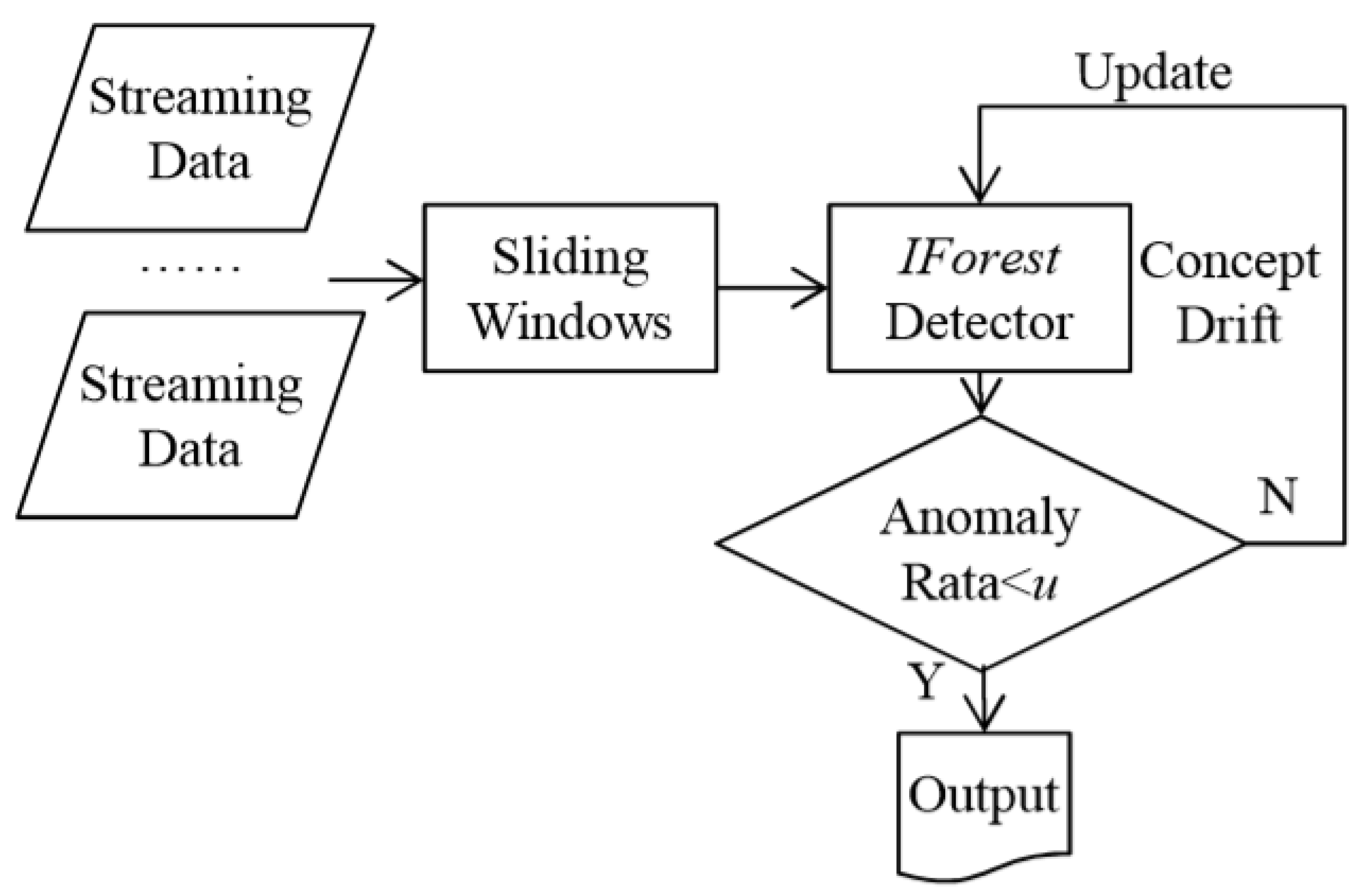
Figure 3.
Isolation Forest ASD algorithm workflow for Drift Detection implemented in scikit-multiflow. Image extracted from the original paper by [Ding & Fei, 2013] [3].
Figure 3.
Isolation Forest ASD algorithm workflow for Drift Detection implemented in scikit-multiflow. Image extracted from the original paper by [Ding & Fei, 2013] [3].

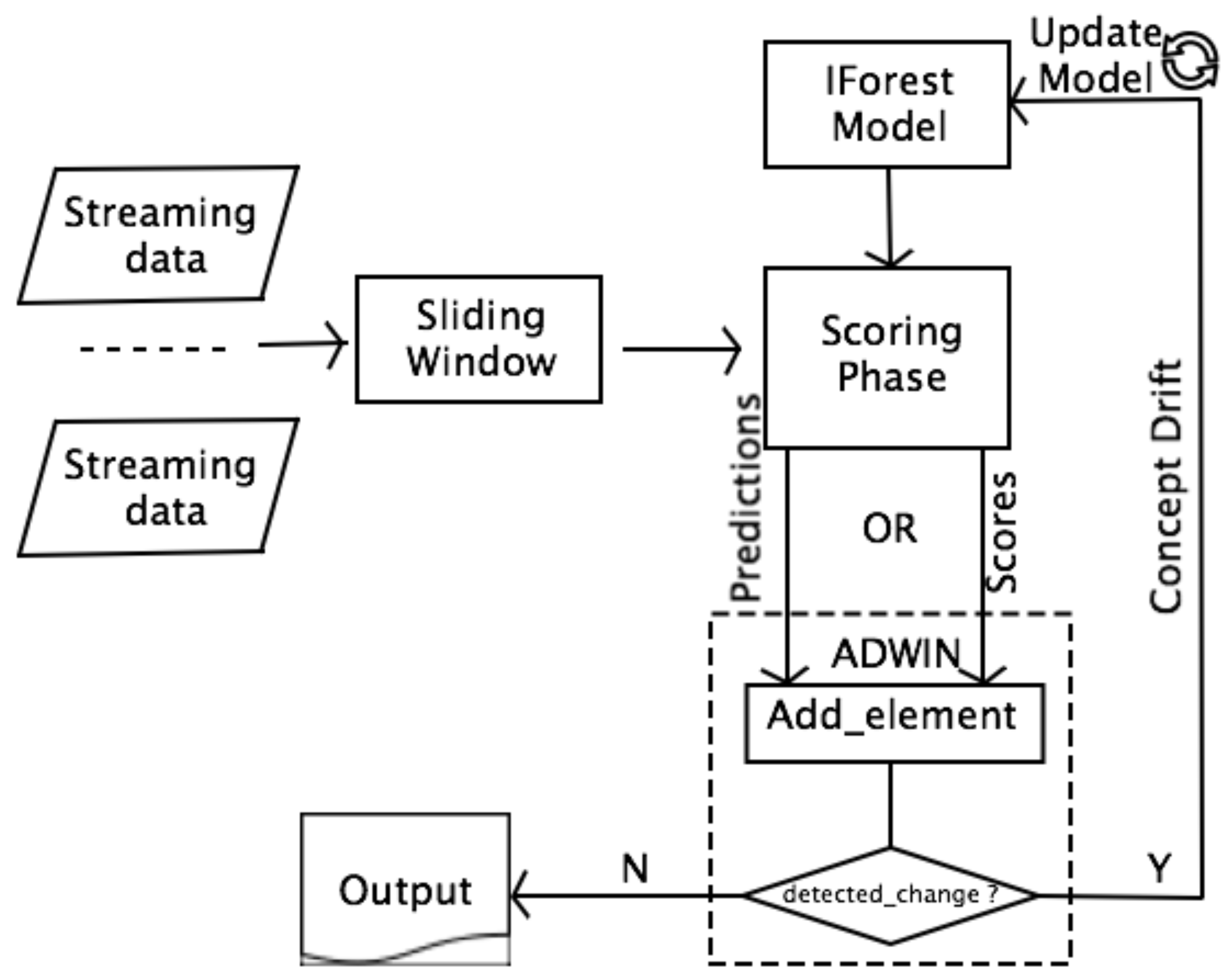
Figure 4.
ADWIN based IForestASD method workflow: PADWIN IFA if predictions are used, SADWIN IFA if scores are considered. Figure inspired from [3].
Figure 4.
ADWIN based IForestASD method workflow: PADWIN IFA if predictions are used, SADWIN IFA if scores are considered. Figure inspired from [3].

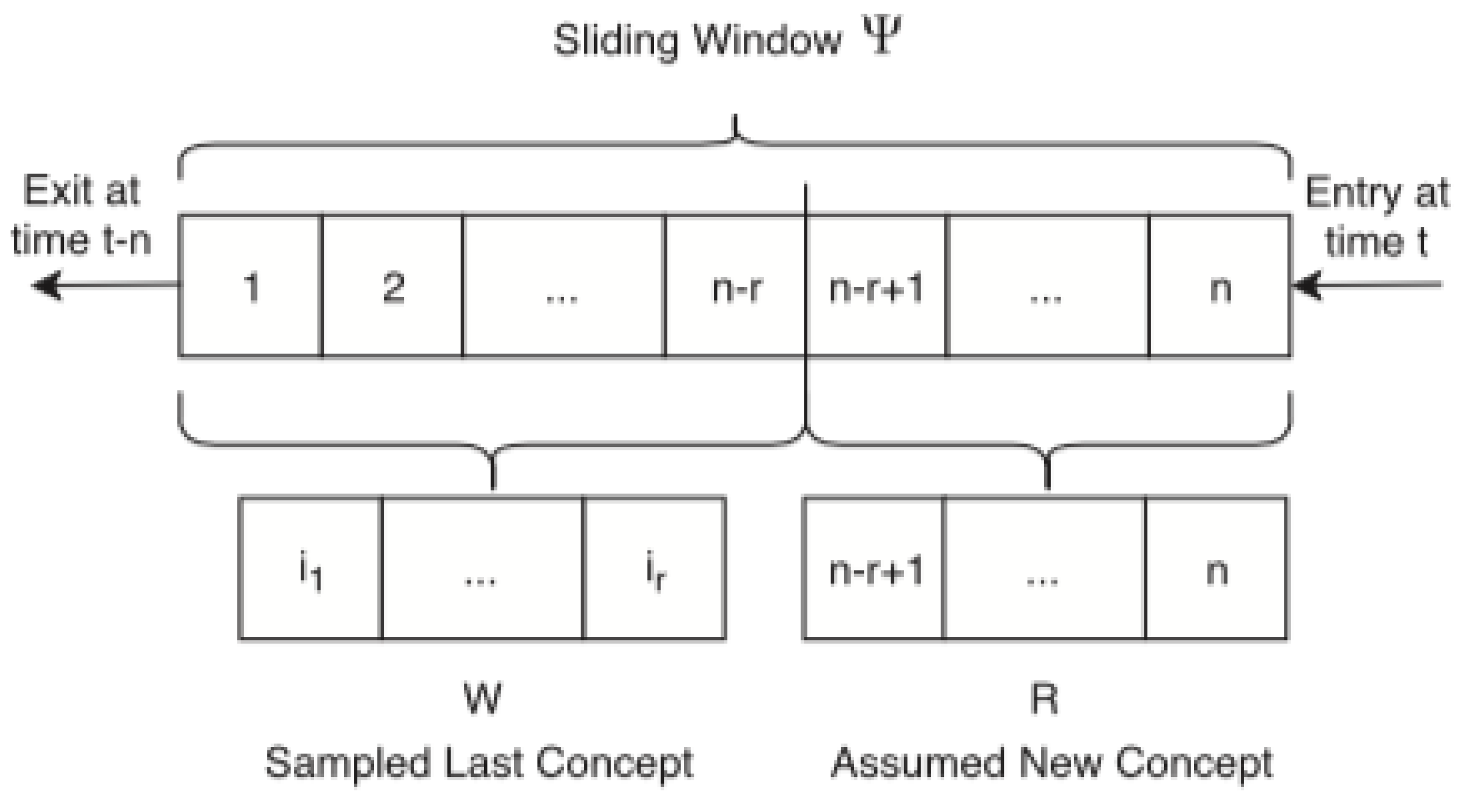
Figure 5.
The memory strategy used by Raab et al. in [5] for the concept drift detector: at every time step, r samples are selected randomly and they are compared against the newest r samples of the window from the stored n samples in a sliding window ().
Figure 5.
The memory strategy used by Raab et al. in [5] for the concept drift detector: at every time step, r samples are selected randomly and they are compared against the newest r samples of the window from the stored n samples in a sliding window ().

Figure 6.
NDKSWIN based IForestASD method workflow (NDKSWIN IFA). Image inspired from [3].
Figure 6.
NDKSWIN based IForestASD method workflow (NDKSWIN IFA). Image inspired from [3].
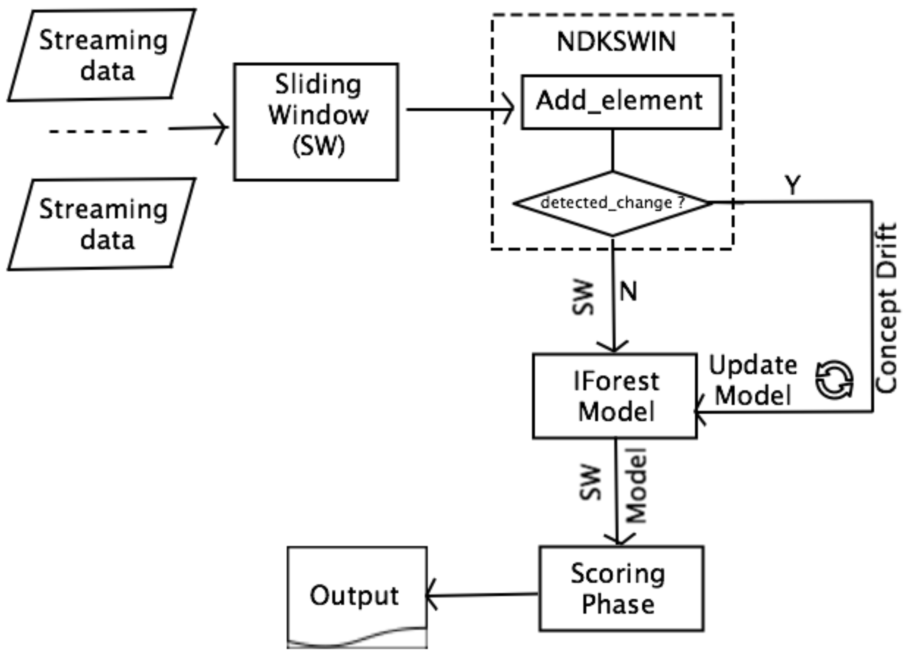
Figure 7.
Impact of window size W and number of trees T on memory consumption (model size metric) for both HSTrees (barplot—left Y axis) with Shuttle and IForestASD (lines—right Y axis) for the three datasets. HST memory consumption is ≈20× bigger than IFA.
Figure 7.
Impact of window size W and number of trees T on memory consumption (model size metric) for both HSTrees (barplot—left Y axis) with Shuttle and IForestASD (lines—right Y axis) for the three datasets. HST memory consumption is ≈20× bigger than IFA.

Figure 8.
Impact of W and T on the Running Time Metric (training and testing time in seconds) for HST and IForestASD, Forest-Cover data set. The IForestASD testing time is represented in another scale on the right Y axis and plotted in red line.
Figure 8.
Impact of W and T on the Running Time Metric (training and testing time in seconds) for HST and IForestASD, Forest-Cover data set. The IForestASD testing time is represented in another scale on the right Y axis and plotted in red line.

Table 1.
Comparison of Anomaly Detection in Data Stream (ADiDS) approaches.
| Approaches | Advantages | Disadvantages |
|---|---|---|
| Statistics-based | Non-parametric methods are adapted to data stream context |
|
| Nearest-neighbors | Distance-based methods
| Distance-based methods
|
Density-based methods
| Density-based methods
| |
| Clustering-based | Adapted for clusters identification | Not optimized for individual anomaly identification |
| Isolation-based |
|
|
Table 2.
Datasets and hyper-parameters set up.
| Shuttle | Forest-Cover | SMTP | SEA | |
|---|---|---|---|---|
| Attributes, Number of features | 9 | 10 | 3 | 3 |
| u—Drift Rate = Anomaly rate | 7.15% | 0.96% | 0.03% | 0.1% |
| Number of samples | 49,097 | 286,048 | 95,156 | 10,000 |
| W—Window size range | [50, 100, 500, 1000] | |||
| T—Number of Trees | [30, 50, 100] |
Table 3.
Comparison between HS-Trees (HST) and IForestASD (IFA). We fixed the window size w (50, 100, 50, 1000) and varied the number of trees T for each dataset Forest Cover, Shuttle, and SMTP (36 configurations)—HRa and IRa represent HSTrees ratio and IFA ratio described in Section 6.1.
Table 3.
Comparison between HS-Trees (HST) and IForestASD (IFA). We fixed the window size w (50, 100, 50, 1000) and varied the number of trees T for each dataset Forest Cover, Shuttle, and SMTP (36 configurations)—HRa and IRa represent HSTrees ratio and IFA ratio described in Section 6.1.
| Forest Cover | Shuttle | SMTP | |||||||||||
|---|---|---|---|---|---|---|---|---|---|---|---|---|---|
| 1 | Time | Size | 1 | Time | Size | 1 | Time | Size | |||||
| HST | IFA | IRa | HRa | HST | IFA | IRa | HRa | HST | IFA | IRa | HRa | ||
| 50 | 30 | 0.36 | 0.22 | 3 | 702 | 0.13 | 0.64 | 3 | 817 | 0 | 0.34 | 3 | 926 |
| 50 | 50 | 0.36 | 0.23 | 3 | 694 | 0.13 | 0.64 | 3 | 854 | 0 | 0.34 | 3 | 940 |
| 50 | 100 | 0.36 | 0.22 | 3 | 737 | 0.13 | 0.64 | 3 | 950 | 0 | 0.34 | 3 | 986 |
| 100 | 30 | 0.39 | 0.30 | 12 | 367 | 0.14 | 0.71 | 12 | 461 | 0 | 0.36 | 9 | 596 |
| 100 | 50 | 0.39 | 0.29 | 12 | 404 | 0.13 | 0.72 | 14 | 505 | 0 | 0.36 | 9 | 734 |
| 100 | 100 | 0.39 | 0.30 | 12 | 416 | 0.13 | 0.71 | 16 | 551 | 0 | 0.36 | 9 | 808 |
| 500 | 30 | 0.39 | 0.49 | 158 | 108 | 0.14 | 0.80 | 519 | 28 | 0 | 0.39 | 106 | 288 |
| 500 | 50 | 0.39 | 0.47 | 152 | 129 | 0.13 | 0.80 | 393 | 36 | 0 | 0.40 | 111 | 372 |
| 500 | 100 | 0.39 | 0.47 | 156 | 140 | 0.15 | 0.80 | 363 | 92 | 0 | 0.40 | 111 | 434 |
| 1000 | 30 | 0.54 | 0.40 | 372 | 63 | 0.17 | 0.78 | 1757 | 21 | 0 | 0.39 | 264 | 127 |
| 1000 | 50 | 0.54 | 0.40 | 387 | 74 | 0.14 | 0.78 | 1175 | 28 | 0 | 0.39 | 272 | 155 |
| 1000 | 100 | 0.55 | 0.40 | 391 | 86 | 0.14 | 0.77 | 1678 | 23 | 0 | 0.39 | 272 | 176 |
Table 4.
Comparison between IForestASD (IFA), SADWIN IFA (SAd), PADWIN IFA (PAd) and NDKSWIN IFA (KSi), on Shuttle, SMTP, and SEA datasets with W = [100, 500] and T = 30.
Table 4.
Comparison between IForestASD (IFA), SADWIN IFA (SAd), PADWIN IFA (PAd) and NDKSWIN IFA (KSi), on Shuttle, SMTP, and SEA datasets with W = [100, 500] and T = 30.
| Shuttle | SMTP | SEA | |||||||||||
|---|---|---|---|---|---|---|---|---|---|---|---|---|---|
| Metrics | W | IFA | SAd | PAd | KSi | IFA | SAd | PAd | KSi | IFA | SAd | PAd | KSi |
| 1 | 100 | 0.72 | 0.74 | 0.73 | 0.70 | 0.37 | 0.33 | 0.33 | 0.34 | 0.41 | 0.39 | 0.42 | 0.41 |
| 500 | 0.80 | 0.81 | 0.80 | 0.80 | 0.41 | 0.40 | 0.39 | 0.39 | 0.39 | 0.40 | 0.39 | 0.38 | |
| Model updated | 100 | 0 | 0 | 0 | 3 | 88 | 6 | 10 | 11 | 99 | 0 | 0 | 7 |
| 500 | 0 | 0 | 0 | 2 | 15 | 3 | 5 | 2 | 19 | 0 | 0 | 2 | |
| Time Ratio | 100 | - | 0.99 | 1.01 | 1.05 | - | 1.09 | 1.03 | 1.08 | - | 1.03 | 1.05 | 1.05 |
| 500 | - | 1.00 | 1.00 | 1.00 | - | 1.07 | 1.09 | 1.10 | - | 1.01 | 1.02 | 1.02 | |
| Size Ratio | 100 | - | 0.94 | 0.97 | 0.94 | - | 1.32 | 1.12 | 1.24 | - | 0.96 | 0.93 | 1.06 |
| 500 | - | 0.97 | 0.98 | 0.98 | - | 0.89 | 1.39 | 1.31 | - | 0.98 | 0.96 | 1.03 | |
Publisher’s Note: MDPI stays neutral with regard to jurisdictional claims in published maps and institutional affiliations. |
© 2021 by the authors. Licensee MDPI, Basel, Switzerland. This article is an open access article distributed under the terms and conditions of the Creative Commons Attribution (CC BY) license (http://creativecommons.org/licenses/by/4.0/).
Share and Cite
MDPI and ACS Style
Togbe, M.U.; Chabchoub, Y.; Boly, A.; Barry, M.; Chiky, R.; Bahri, M. Anomalies Detection Using Isolation in Concept-Drifting Data Streams . Computers 2021, 10, 13. https://0-doi-org.brum.beds.ac.uk/10.3390/computers10010013
AMA Style
Togbe MU, Chabchoub Y, Boly A, Barry M, Chiky R, Bahri M. Anomalies Detection Using Isolation in Concept-Drifting Data Streams . Computers. 2021; 10(1):13. https://0-doi-org.brum.beds.ac.uk/10.3390/computers10010013
Chicago/Turabian StyleTogbe, Maurras Ulbricht, Yousra Chabchoub, Aliou Boly, Mariam Barry, Raja Chiky, and Maroua Bahri. 2021. "Anomalies Detection Using Isolation in Concept-Drifting Data Streams " Computers 10, no. 1: 13. https://0-doi-org.brum.beds.ac.uk/10.3390/computers10010013
Note that from the first issue of 2016, this journal uses article numbers instead of page numbers. See further details here.