Trading-Off Machine Learning Algorithms towards Data-Driven Administrative-Socio-Economic Population Health Management

 ,
,  ,
,
Abstract
:1. Introduction
2. Related Works
3. Materials and Methods
3.1. Data Pre-Processing
- Diagnoses were grouped by single-level Clinical Classification Software (CCS) [55]. They are 283 clinically homogeneous mutually exclusive categories, which cluster all the 14,000 diagnosis codes, according to International Classification of Diseases, 9th Revision, Clinical Modification (ICD-9-CM, Fifth Edition) [56]. We counted the number of hospital admissions and summed the number of days of hospitalisation for each CCS for each patient for different dates. For example, if patient A has been hospitalised on 1st January 2014 for 3 days with ICD-9-CM codes 250.60 (diabetes with neurological manifestations, type II or unspecified type, not stated as uncontrolled), 250.70 (diabetes with peripheral circulatory disorders, type II or unspecified type, not stated as uncontrolled) and 278.00 (obesity), since the two codes 250.60 and 250.70 belong to CCS 50 (diabetes mellitus with complications) and the code 278.00 belongs to CCS 58 (other nutritional endocrine and metabolic disorders), this event counts as 1 hospital admission with 3 days of hospitalisation for CSS 50 and 1 hospital admission with 3 days of hospitalisation for CCS 58. Another admission of 5 days with code 250.60 on 30th March 2014 for the same patient will be summed to the previous one for CCS 50, for a total of 2 hospital admissions and 8 days of hospitalisation for CCS 50 for patient A. Considering admissions and days as two different variables for each CCS, the total number of input attributes for diagnoses was 566.
- Procedures were grouped by single-level CCS. For procedure classification, the scheme contains 231 mutually exclusive categories, grouping 3900 ICD-9-CM procedure codes [57]. The ICD-9-CM codes of each category usually refer to the same system/organ. The number of procedures done for each CCS for each patient on different dates was counted. The total number of input features for procedures was then 231.
- Outpatient services were divided into 76 ad-hoc groups. The outpatient services codes are about 2000, but a unique regrouping method is not defined yet. Therefore, they were divided first in visits, diagnostics, laboratory, therapeutics and rehabilitation and then we went into more detail, considering criteria like methods and purpose, defining 76 mutually exclusive and homogeneous ad-hoc groups. The services made on different dates for every group and every patient were counted. Each group represented an input variable, for a total of 76 variables.
- For drugs, Anatomical Therapeutic Chemical classification system (ATC) [58] was chosen. The third level (ATC3) was selected for classification. It is the therapeutic/pharmacological subgroup of the drug itself and it is usually used to identify 265 therapeutic subgroups of about 3350 chemical substances. The number of drugs taken in the period for different ATC3 classes and on different dates was counted, for a total of 265 attributes for drugs.
- Exemptions were partitioned into 28 ad-hoc mutually exclusive groups. Starting from almost 800 codes, the classification was done considering the motivation of the exemption, according to chronic diseases, specific services (e.g., emergency room or sports medicine) and income. Every class was a categorical variable (for a total of 28 input features) with three values: “0” for no exemptions for the group, “1” meaning at least an active exemption for the group at 1st January 2015, and “2” if the exemption has expired during the period of study.
3.2. Modelling and Feature Selection
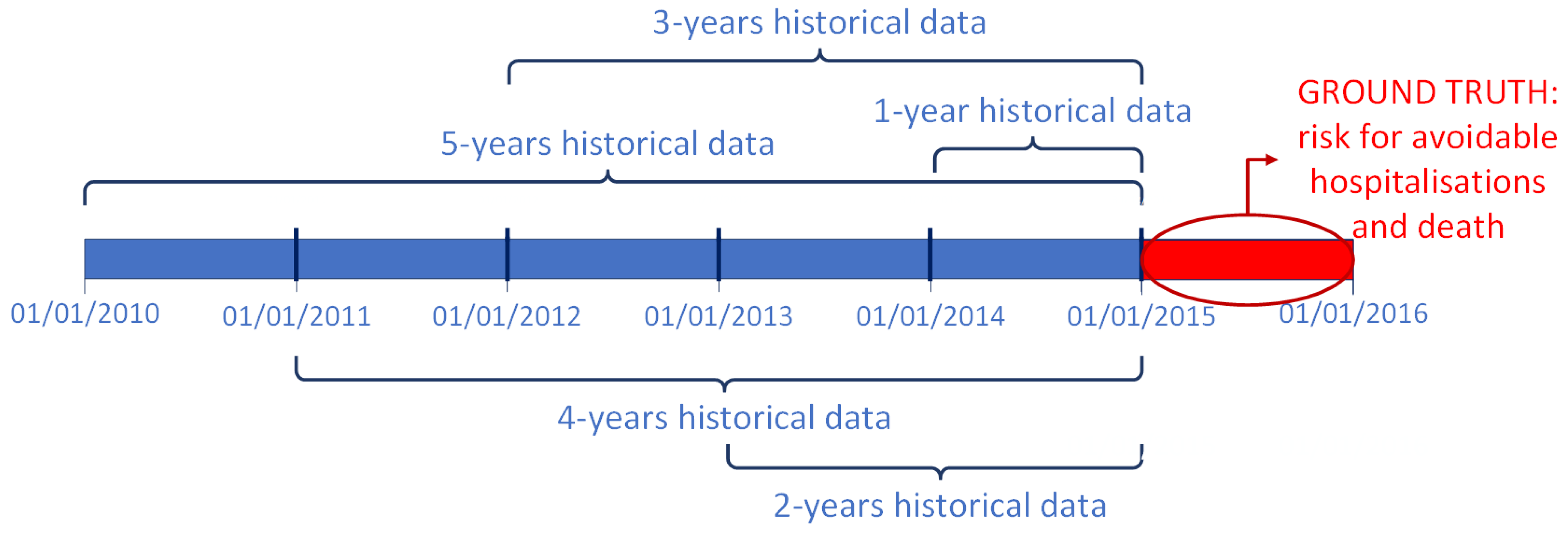
- for the 5-years dataset, 280 variables were confirmed as important (99 diagnoses, 58 procedures, 35 outpatient services, 80 drugs, 6 exemptions, age and gender);
- for the 4-years dataset, 225 features were selected as important (65 diagnoses, 38 procedures, 38 outpatient services, 76 drugs, 6 exemptions, age and gender);
- for the 3-years dataset, 244 variables were chosen (58 diagnoses, 62 procedures, 39 outpatient services, 74 drugs, 9 exemptions, age and gender);
- for the 2-years dataset, 199 attributes were confirmed as important (47 diagnoses, 39 procedures, 29 outpatient services, 71 drugs, 11 exemptions, age and gender);
- for the 1-year dataset, 153 features were selected as important (44 diagnoses, 23 procedures, 24 outpatient services, 54 drugs, 6 exemptions, age and gender).
4. Results
5. Discussion
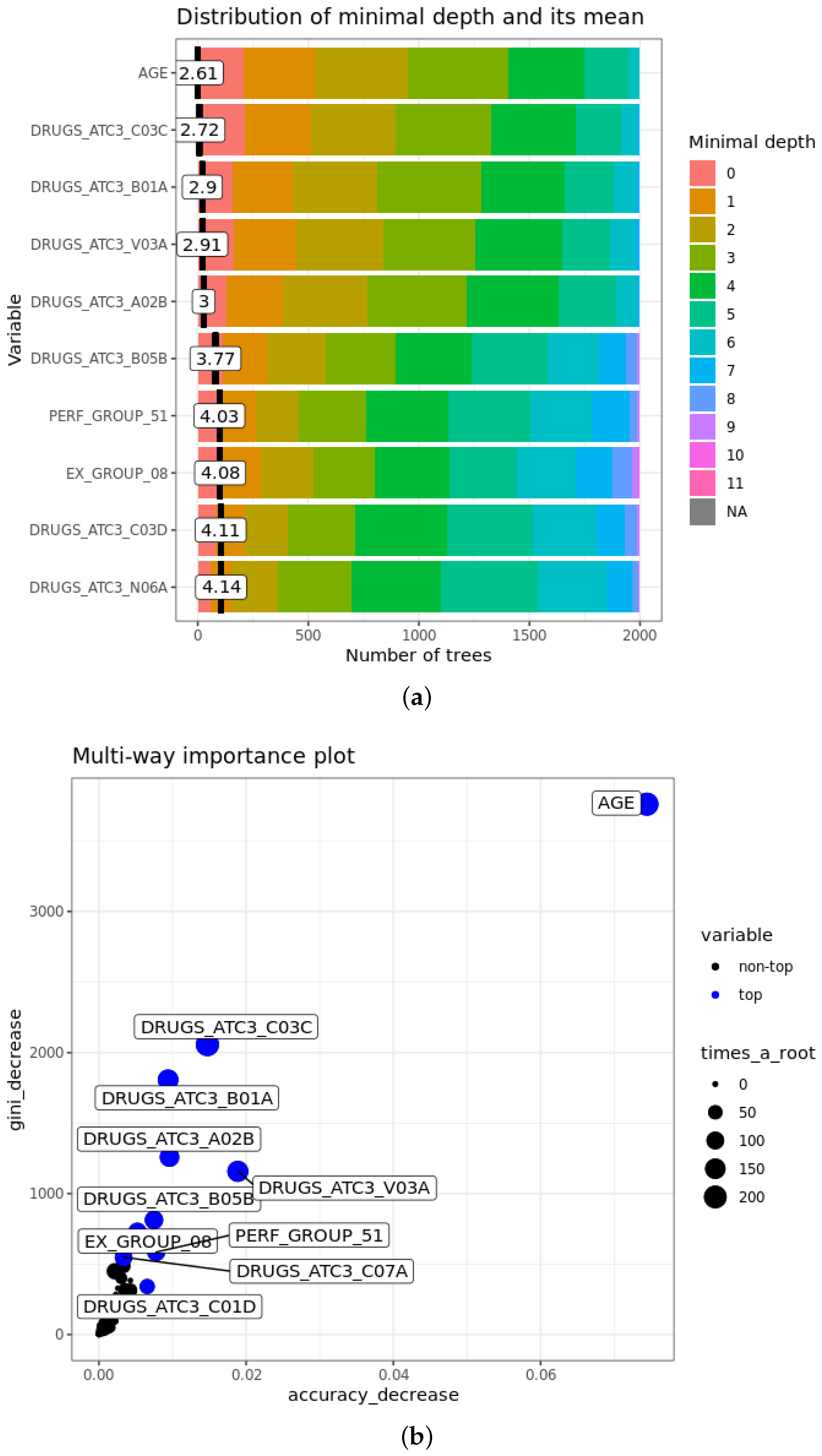
- The mean minimal depth of A is the average of the minimal depth of A in each tree, where the minimal depth of A in each tree represents the length of the path from the root to the node where the variable A is used for splitting. The more important the feature is, the smaller mean minimal depth is, since it means that the variable discriminates well the two classes, maximising the reduction of impurity in the set.
- of A is the number of trees where the variable A is at the root. Obviously, it is strongly related inversely to the mean minimal depth: with the growth of , mean minimal depth decreases.
- Accuracy decrease for variable A is the mean decrease of accuracy in predictions if A is randomly permuted. If it is larger, the variable is more important and affects more the final predictions.
- Gini decrease of A is the mean decrease of Gini index when splitting on A itself. As for accuracy decrease, the larger it is, the greater is the weight of the attribute in the predictions.
6. Conclusions
Author Contributions
Funding
Institutional Review Board Statement
Informed Consent Statement
Data Availability Statement
Conflicts of Interest
References
- Mitchell, E.; Walker, R. Global ageing: Successes, challenges and opportunities. Br. J. Hosp. Med. 2020, 81. [Google Scholar] [CrossRef] [PubMed]
- Anderson, G.F.; Hussey, P.S. Population Aging: A Comparison Among Industrialized Countries. Health Aff. 2000, 19. [Google Scholar] [CrossRef] [PubMed]
- Colby, S.L.; Ortman, J.M. Projections of the Size and Composition of the U.S. Population: 2014 to 2060. Population Estimates and Projections; Current Population Reports; Census Bureau: Washington, DC, USA, 2015.
- Nash, A. National Population Projections: 2018-Based. 2019. Available online: www.ons.gov.uk/peoplepopulationandcommunity/populationandmigration/populationprojections/bulletins/nationalpopulationprojections2018based (accessed on 29 November 2020).
- Légaré, J. Population Aging: Economic and Social Consequences. In International Encyclopedia of the Social & Behavioral Sciences, 2nd ed.; Elsevier: Oxford, UK, 2015; pp. 540–544. [Google Scholar] [CrossRef]
- Kingston, A.; Robinson, L.; Booth, H.; Knapp, M.; Jagger, C. Projections of multi-morbidity in the older population in England to 2035: Estimates from the Population Ageing and Care Simulation (PACSim) model. Age Ageing 2018, 47, 374–380. [Google Scholar] [CrossRef] [PubMed] [Green Version]
- Marengoni, A.; Angleman, S.; Melis, R.; Mangialasche, F.; Karp, A.; Garmen, A.; Meinow, B.; Fratiglioni, L. Aging with multimorbidity: A systematic review of the literature. Ageing Res. Rev. 2011, 10, 430–439. [Google Scholar] [CrossRef] [PubMed]
- Thavorn, K.; Maxwell, C.J.; Gruneir, A.; Bronskill, S.E.; Bai, Y.; Koné Pefoyo, A.J.; Petrosyan, Y.; Wodchis, W.P. Effect of socio-demographic factors on the association between multimorbidity and healthcare costs: A population-based, retrospective cohort study. BMJ Open 2017, 7. [Google Scholar] [CrossRef] [Green Version]
- Bodenheimer, T.; Wagner, E.H.; Grumbach, K. Improving Primary Care for Patients with Chronic Illness. JAMA 2002, 288, 1775–1779. [Google Scholar] [CrossRef]
- Boehmer, K.R.; Dabrh, A.M.A.; Gionfriddo, M.R.; Erwin, P.J.; Montori, V.M. Does the chronic care model meet the emerging needs of people living with multimorbidity? A systematic review and thematic synthesis. PLoS ONE 2018, 13, e0190852. [Google Scholar] [CrossRef] [Green Version]
- Shadmi, E.; Freund, T. Targeting patients for multimorbid care management interventions: The case of equity in high-risk patient identification. Int. J. Equity Health 2013, 12. [Google Scholar] [CrossRef] [Green Version]
- Safford, M.M.; Allison, J.J.; Kiefe, C.I. Patient Complexity: More Than Comorbidity. The Vector Model of Complexity. J. Gen. Intern. Med. 2007, 22, 382–390. [Google Scholar] [CrossRef] [Green Version]
- Andreu-Perez, J.; Poon, C.C.Y.; Merrifield, R.D.; Wong, S.T.C.; Yang, G.Z. Big Data for Health. IEEE J. Biomed. Health Inform. 2015, 19, 1193–1208. [Google Scholar] [CrossRef]
- Bates, D.W.; Saria, S.; Ohno-Machado, L.; Shah, A.; Escobar, G. Big Data in Health Care: Using Analytics to Identify And Manage High-Risk and High-Cost Patients. Health Aff. 2014, 33, 1123–1131. [Google Scholar] [CrossRef] [PubMed] [Green Version]
- Raghupathi, W.; Raghupathi, V. Big Data in Healthcare: Promise and Potential. Health Inf. Sci. Syst. 2014, 2. [Google Scholar] [CrossRef] [PubMed]
- Dash, S.; Shakyawar, S.K.; Sharma, M.; Kaushik, S. Big data in healthcare: Management, analysis and future prospects. J. Big Data 2019, 6, 1–25. [Google Scholar] [CrossRef] [Green Version]
- Bresnick, J. How to Get Started with a Population Health Management Program. 2016. Available online: healthitanalytics.com/features/how-to-get-started-with-a-population-health-management-program (accessed on 29 November 2020).
- Panicacci, S.; Donati, M.; Fanucci, L.; Bellini, I.; Profili, F.; Francesconi, P. Population Health Management Exploiting Machine Learning Algorithms to Identify High-Risk Patients. In Proceedings of the 2018 IEEE 31st International Symposium on Computer-Based Medical Systems (CBMS), Karlstad, Sweden, 18–21 June 2018; pp. 298–303. [Google Scholar] [CrossRef]
- Mehta, N.; Pandit, A. Concurrence of big data analytics and healthcare: A systematic review. Int. J. Med. Inform. 2018, 114, 57–65. [Google Scholar] [CrossRef] [PubMed]
- Swain, A.K. Mining big data to support decision making in healthcare. J. Inf. Technol. Case Appl. Res. 2016, 18, 141–154. [Google Scholar] [CrossRef]
- Chen, M.; Hao, Y.; Hwang, K.; Wang, L.; Wang, L. Disease Prediction by Machine Learning over Big Data from Healthcare Communities. IEEE Access 2017, 5, 8869–8879. [Google Scholar] [CrossRef]
- Meng, X.H.; Huang, Y.X.; Rao, D.P.; Zhang, Q.; Liu, Q. Comparison of three data mining models for predicting diabetes or prediabetes by risk factors. Kaohsiung J. Med. Sci. 2013, 29, 93–99. [Google Scholar] [CrossRef] [Green Version]
- Worachartcheewan, A.; Shoombuatong, W.; Pidetcha, P.; Nopnithipat, W.; Prachayasittikul, V.; Nantasenamat, C. Predicting Metabolic Syndrome Using the Random Forest Method. Sci. World J. 2015. [Google Scholar] [CrossRef] [Green Version]
- Latha, C.B.C.; Jeeva, S.C. Improving the accuracy of prediction of heart disease risk based on ensemble classification techniques. Inform. Med. Unlocked 2019, 16. [Google Scholar] [CrossRef]
- Dinesh, K.G.; Arumugaraj, K.; Santhosh, K.D.; Mareeswari, V. Prediction of Cardiovascular Disease Using Machine Learning Algorithms. In Proceedings of the 2018 International Conference on Current Trends towards Converging Technologies (ICCTCT), Coimbatore, India, 1–3 March 2018; pp. 1–7. [Google Scholar] [CrossRef]
- Panicacci, S.; Donati, M.; Fanucci, L.; Bellini, I.; Profili, F.; Francesconi, P. Exploring Machine Learning Algorithms to Identify Heart Failure Patients: The Tuscany Region Case Study. In Proceedings of the 2019 IEEE 32nd International Symposium on Computer-Based Medical Systems (CBMS), Cordoba, Spain, 5–7 June 2019; pp. 417–422. [Google Scholar] [CrossRef]
- Tengnah, M.A.J.; Sooklall, R.; Nagowah, S.D. Chapter 9-A Predictive Model for Hypertension Diagnosis Using Machine Learning Techniques. In Telemedicine Technologies; Academic Press: New York, NY, USA, 2019; pp. 139–152. [Google Scholar] [CrossRef]
- Yang, H.; Bath, P.A. The Use of Data Mining Methods for the Prediction of Dementia: Evidence from the English Longitudinal Study of Aging. IEEE J. Biomed. Health Inform. 2020, 24, 345–353. [Google Scholar] [CrossRef]
- Cattelani, L.; Murri, M.B.; Chesani, F.; Chiari, L.; Bandinelli, S.; Palumbo, P. Risk Prediction Model for Late Life Depression: Development and Validation on Three Large European Datasets. IEEE J. Biomed. Health Inform. 2019, 23, 2196–2204. [Google Scholar] [CrossRef] [PubMed]
- What Is Electronic Health Record (EHR)? 2019. Available online: https://www.healthit.gov/faq/what-electronic-health-record-ehr (accessed on 29 November 2020).
- Myers, L.; Stevens, J. Using EHR to Conduct Outcome and Health Services Research. In Secondary Analysis of Electronic Health Records; Springer International Publishing: Cham, Switzerland, 2016; pp. 61–70. [Google Scholar] [CrossRef] [Green Version]
- Alamri, A. Ontology Middleware for Integration of IoT Healthcare Information Systems in EHR Systems. Computers 2018, 7, 51. [Google Scholar] [CrossRef] [Green Version]
- Hammond, R.; Athanasiadou, R.; Curado, S.; Aphinyanaphongs, Y.; Abrams, C.; Messito, M.; Gross, R.; Katzow, M.; Jay, M.; Razavian, N.; et al. Predicting childhood obesity using electronic health records and publicly available data. PLoS ONE 2019, 14. [Google Scholar] [CrossRef] [PubMed]
- Anderson, J.P.; Parikh, J.R.; Shenfeld, D.K.; Ivanov, V.; Marks, C.; Church, B.W.; Laramie, J.M.; Mardekian, J.; Piper, B.A.; Willke, R.J.; et al. Reverse Engineering and Evaluation of Prediction Models for Progression to Type 2 Diabetes: An Application of Machine Learning Using Electronic Health Records. J. Diabetes Sci. Technol. 2016, 10, 6–18. [Google Scholar] [CrossRef] [Green Version]
- Panahiazar, M.; Taslimitehrani, V.; Pereira, N.; Pathak, J. Using EHRs and Machine Learning for Heart Failure Survival Analysis. Stud. Health Technol. Inform. 2015, 216, 40–44. [Google Scholar]
- Pike, M.M.; Decker, P.A.; Larson, N.B.; Sauver, J.L.S.; Takahashi, P.Y.; Roger, V.L.; Rocca, W.A.; Miller, V.M.; Olson, J.E.; Pathak, J.; et al. Improvement in Cardiovascular Risk Prediction with Electronic Health Records. J. Cardiovasc. Transl. Res. 2016, 9, 214–222. [Google Scholar] [CrossRef]
- Sun, J.; McNaughton, C.D.; Zhang, P.; Perer, A.; Gkoulalas-Divanis, A.; Denny, J.C.; Kirby, J.; Lasko, T.; Saip, A.; Malin, B.A. Predicting changes in hypertension control using electronic health records from a chronic disease management program. J. Am. Med. Inform. Assoc. 2013, 21, 337–344. [Google Scholar] [CrossRef] [Green Version]
- Barnes, D.E.; Zhou, J.; Walker, R.L.; Larson, E.B.; Lee, S.J.; Boscardin, W.J.; Marcum, Z.A.; Dublin, S. Development and Validation of eRADAR: A Tool Using EHR Data to Detect Unrecognized Dementia. J. Am. Geriatr. Soc. 2020, 68, 103–111. [Google Scholar] [CrossRef]
- Jin, Z.; Cui, S.; Guo, S.; Gotz, D.; Sun, J.; Cao, N. CarePre: An Intelligent Clinical Decision Assistance System. ACM Trans. Comput. Healthc. 2020, 1. [Google Scholar] [CrossRef] [Green Version]
- Morawski, K.; Dvorkis, Y.; Monsen, C.B. Predicting Hospitalizations from Electronic Health Record Data. Am. J. Manag. Care 2020. [Google Scholar] [CrossRef]
- Miotto, R.; Li, L.; Dudley, J.T. Deep Learning to Predict Patient Future Diseases from the Electronic Health Records. In Advances in Information Retrieval; Springer International Publishing: Cham, Switzerland, 2016; pp. 768–774. [Google Scholar]
- Kim, Y.J.; Park, H. Improving Prediction of High-Cost Health Care Users with Medical Check-Up Data. Big Data 2019, 7. [Google Scholar] [CrossRef] [PubMed]
- Shenas, S.A.I.; Raahemi, B.; Tekieh, M.H.; Kuziemsky, C. Identifying high-cost patients using data mining techniques and a small set of non-trivial attributes. Comput. Biol. Med. 2014, 53, 9–18. [Google Scholar] [CrossRef] [PubMed]
- Morid, M.A.; Kawamoto, K.; Ault, T.; Dorius, J.; Abdelrahman, S. Supervised Learning Methods for Predicting Healthcare Costs: Systematic Literature Review and Empirical Evaluation. Amia Annu. Symp. Proc. 2017, 2017, 1312–1321. [Google Scholar] [PubMed]
- Bellini, I.; Barletta, V.R.; Profili, F.; Bussotti, A.; Severi, I.; Isoldi, M.; Bimbi, M.V.F.; Francesconi, P. Identifying High-Cost, High-Risk Patients Using Administrative Databases in Tuscany, Italy. BioMed Res. Int. 2017. [Google Scholar] [CrossRef] [Green Version]
- Louis, D.Z.; Robeson, M.; McAna, J.; Maio, V.; Keith, S.W.; Liu, M.; Gonnella, J.S.; Grilli, R. Predicting risk of hospitalisation or death: A retrospective population-based analysis. BMJ Open 2014, 4. [Google Scholar] [CrossRef] [PubMed] [Green Version]
- Balzi, D.; Carreras, G.; Tonarelli, F.; Degli Esposti, L.; Michelozzi, P.; Ungar, A.; Gabbani, L.; Benvenuti, E.; Landini, G.; Bernabei, R.; et al. Real-time utilisation of administrative data in the ED to identify older patients at risk: Development and validation of the Dynamic Silver Code. BMJ Open 2019, 9. [Google Scholar] [CrossRef] [Green Version]
- Linn, S.; Grunau, P.D. New patient-oriented summary measure of net total gain in certainty for dichotomous diagnostic tests. Epidemiol. Perspect. Innvoation 2006, 3. [Google Scholar] [CrossRef] [Green Version]
- Sokolova, M.; Lapalme, G. A systematic analysis of performance measures for classification tasks. Inf. Process. Manag. 2009, 45, 427–437. [Google Scholar] [CrossRef]
- Tutela Delle Persone e di Altri Soggetti Rispetto al Trattamento dei dati Personali [Protection of Persons and Other Subjects with Regard to Personal Data Processing]. 1996. Available online: http://www.garanteprivacy.it/web/guest/home/docweb/-/docwebdisplay/docweb/28335 (accessed on 29 November 2020).
- Donatini, A. The Italian Health Care System. 2020. Available online: https://international.commonwealthfund.org/countries/italy/ (accessed on 29 November 2020).
- ISTAT. Available online: https://www.istat.it/ (accessed on 29 November 2020).
- Toscana, A.R.S. MARSupio Database. 2018. Available online: https://www.ars.toscana.it/marsupio/database/ (accessed on 29 November 2020).
- AHRQ. Potentially Avoidable Hospitalizations. 2018. Available online: www.ahrq.gov/research/findings/nhqrdr/chartbooks/carecoordination/measure3.html (accessed on 29 November 2020).
- Elixhauser, A.; Steiner, C.; Palmer, L. Clinical Classification Software (CCS). 2016. Available online: http://www.hcup-us.ahrq.gov/toolssoftware/ccs/ccs.jsp (accessed on 29 November 2020).
- ICD-9-CM Diagnosis Codes. Available online: www.icd9data.com/2012/Volume1/default.htm (accessed on 29 November 2020).
- ICD-9-CM Procedure Codes. Available online: www.icd9data.com/2012/Volume3/default.htm (accessed on 29 November 2020).
- WHOCC. Anatomical Therapeutic Chemical Classification System (ATC). 2018. Available online: www.whocc.no/atc/structure_and_principles/ (accessed on 29 November 2020).
- HealthCatalyst. Population Health Management: Systems and Success. 2017. Available online: https://www.healthcatalyst.com/population-health/ (accessed on 29 November 2020).
- Eurostat. Projected Old-Age Dependency Ratio. 2019. Available online: https://ec.europa.eu/eurostat/web/products-datasets/-/tps00200 (accessed on 29 November 2020).
- Brownlee, J. 8 Tactics to Combat Imbalanced Classes in Your Machine Learning Dataset. 2015. Available online: machinelearningmastery.com/tactics-to-combat-imbalanced-classes-in-your-machine-learning-dataset/ (accessed on 29 November 2020).
- Breiman, L.; Friedman, J.; Olsen, R.A.; Stone, C.J. Classification and Regression Trees; Wadsworth International Group: Belmont, CA, USA, 1984. [Google Scholar]
- Therneau, T.; Atkinson, B.; Ripley, B. Package ‘Rpart’. 2019. Available online: https://cran.r-project.org/web/packages/rpart/rpart.pdf (accessed on 29 November 2020).
- Pandya, R.; Pandya, J. C5.0 Algorithm to Improved Decision Tree with Feature Selection and Reduced Error Pruning. Int. J. Comput. Appl. 2015, 117, 18–21. [Google Scholar] [CrossRef]
- Kuhn, M.; Weston, S.; Culp, M.; Coulter, N.; Quinlan, R. Package ‘C50’. 2020. Available online: https://cran.r-project.org/web/packages/C50/C50.pdf (accessed on 29 November 2020).
- Hothorn, T.; Hornik, K.; Zeileis, A. Unbiased Recursive Partitioning: A Conditional Inference Framework. J. Comput. Graph. Stat. 2006, 15, 651–674. [Google Scholar] [CrossRef] [Green Version]
- Hothorn, T.; Hornik, K.; Strobl, C.; Zeileis, A. Package ‘Party’. 2020. Available online: https://cran.r-project.org/web/packages/party/party.pdf (accessed on 29 November 2020).
- Breiman, L. Random Forests. Mach. Learn. 2001, 45, 5–32. [Google Scholar] [CrossRef] [Green Version]
- Wright, M.N.; Wager, S.; Probst, P. Package ‘Ranger’. 2020. Available online: https://cran.r-project.org/web/packages/ranger/ranger.pdf (accessed on 29 November 2020).
- Maind, S.B.; Wankar, P. Research Paper on Basic of Artificial Neural Network. Int. J. Recent Innov. Trends Comput. Commun. 2014, 2, 96–100. [Google Scholar]
- Ripley, B.; Venables, W. Package ‘nnet’. 2020. Available online: https://cran.r-project.org/web/packages/nnet/nnet.pdf (accessed on 29 November 2020).
- Tibshirani, R. Regression Shrinkage and Selection via the Lasso. J. R. Stat. Soc. Ser. B (Methodol.) 1996, 58, 267–288. [Google Scholar] [CrossRef]
- Friedman, J.; Hastie, T.; Tibshirani, R.; Narasimhan, B.; Simon, N.; Qian, J. Package ‘glmnet’. 2020. Available online: https://cran.r-project.org/web/packages/glmnet/glmnet.pdf (accessed on 29 November 2020).
- Kursa, M.B.; Jankowski, A.; Rudnicki, W.R. Boruta—A System for Feature Selection. Fundam. Inform. 2010, 101. [Google Scholar] [CrossRef]
- Donati, M.; Celli, A.; Ruiu, A.; Saponara, S.; Fanucci, L. A Telemedicine Service System Exploiting BT/BLE Wireless Sensors for Remote Management of Chronic Patients. Technologies 2019, 7, 13. [Google Scholar] [CrossRef] [Green Version]
- Altman, D.G.; Bland, J.M. Statistics Notes: Diagnostic tests 2: Predictive values. BMJ 1994, 309, 102. [Google Scholar] [CrossRef] [Green Version]
- Paluszynska, A.; Biecek, P.; Jiang, Y. Package ‘RandomForestExplainer’. 2020. Available online: https://cran.r-project.org/web/packages/randomForestExplainer/randomForestExplainer.pdf (accessed on 29 November 2020).


| Class | Codes | Grouping Method | Groups | Input Variables |
|---|---|---|---|---|
| Diagnoses | ∼14,000 | CCS | 283 | 566 |
| Procedures | ∼3900 | CCS | 231 | 231 |
| Outpatient Services | ∼2000 | Ad-hoc | 76 | 76 |
| Drugs | ∼3350 | ATC3 | 265 | 265 |
| Exemptions | ∼800 | Ad-hoc | 28 | 28 |
| Class | Input Variables | |
|---|---|---|
| Medical Variables | Diagnoses | 566 |
| Procedures | 231 | |
| Outpatient Services | 76 | |
| Drugs | 265 | |
| Exemptions | 28 | |
| Socio-Economic Variables | Personal | 2 |
| Municipality of residence | 3 | |
| Census Section of residence | 7 | |
| Total | 1178 | |
| Class | Complete Dataset | Initial Training Set | Balanced Training Set | Test Set | ||||
|---|---|---|---|---|---|---|---|---|
| Samples | % | Samples | % | Samples | % | Samples | % | |
| 5-years | ||||||||
| B | 21,711 | 1.42 | 15,198 | 1.42 | 15,198 | 22.36 | 6513 | 1.42 |
| G | 1,508,003 | 98.58 | 1,055,603 | 98.58 | 52,780 | 77.64 | 452,400 | 98.58 |
| 4-years | ||||||||
| B | 21,963 | 1.39 | 15,375 | 1.39 | 15,375 | 21.98 | 6588 | 1.39 |
| G | 1,558,936 | 98.61 | 1,091,256 | 98.61 | 54,562 | 78.02 | 467,680 | 98.61 |
| 3-years | ||||||||
| B | 22,033 | 1.37 | 15,424 | 1.37 | 15,424 | 21.77 | 6609 | 1.37 |
| G | 1,583,594 | 98.63 | 1,108,516 | 98.63 | 55,425 | 78.23 | 475,078 | 98.63 |
| 2-years | ||||||||
| B | 22,083 | 1.36 | 15,459 | 1.36 | 15,459 | 21.55 | 6624 | 1.36 |
| G | 1,607,568 | 98.64 | 1,125,298 | 98.64 | 56,264 | 78.45 | 482,270 | 98.64 |
| 1-year | ||||||||
| B | 22,119 | 1.34 | 15,484 | 1.34 | 15,484 | 21.38 | 6635 | 1.34 |
| G | 1,626,778 | 98.66 | 1,138,745 | 98.66 | 56,937 | 78.62 | 488,033 | 98.66 |
| Algorithm | Parameters and Ranges | Training Set | Best Values before FS | Best Values after FS |
|---|---|---|---|---|
| CART | in [10, 10, 10, 10, 10] in [50, 70, 100, 150, 200] | 5-years | (10, 200) | (10, 100) |
| 4-years | (10, 200) | (10, 150) | ||
| 3-years | (10, 100) | (10, 100) | ||
| 2-years | (10, 100) | (10, 100) | ||
| 1-year | (10, 70) | (10, 70) | ||
| C5.0 | in [50, 70, 100, 150, 200] | 5-years | 50 | 50 |
| 4-years | 50 | 50 | ||
| 3-years | 50 | 50 | ||
| 2-years | 50 | 50 | ||
| 1-year | 50 | 50 | ||
| CTree | in [50, 70, 100, 150, 200] | 5-years | 200 | 200 |
| 4-years | 50 | 70 | ||
| 3-years | 50 | 50 | ||
| 2-years | 70 | 50 | ||
| 1-year | 70 | 50 | ||
| RF | in [300, 500, 700, 1000, 1500, 2000] in [10, 16, 24, 34] | 5-years | (1000, 34) | (1000, 34) |
| 4-years | (500, 34) | (500, 24) | ||
| 3-years | (500, 34) | (500, 24) | ||
| 2-years | (800, 34) | (800, 34) | ||
| 1-year | (2000, 34) | (2000, 16) | ||
| ANN | in [2, 3, 4, ..., 13, 14, 15] | 5-years | 10 | 13 |
| 4-years | 11 | 14 | ||
| 3-years | 8 | 12 | ||
| 2-years | 5 | 6 | ||
| 1-year | 9 | 13 | ||
| LASSO | in [4.6 × 10, 2.6 × 10, 1.5 × 10, 1.4 × 10, 1.2 × 10, 7.8 × 10, 5.3 × 10, 4.9 × 10, 3.3 × 10] | 5-years | 1.5 × 10 | 4.9 × 10 |
| 4-years | 4.6 × 10 | 3.3 × 10 | ||
| 3-years | 1.2 × 10 | 7.8 × 10 | ||
| 2-years | 1.4 × 10 | 3.3 × 10 | ||
| 1-year | 2.6 × 10 | 5.3 × 10 |
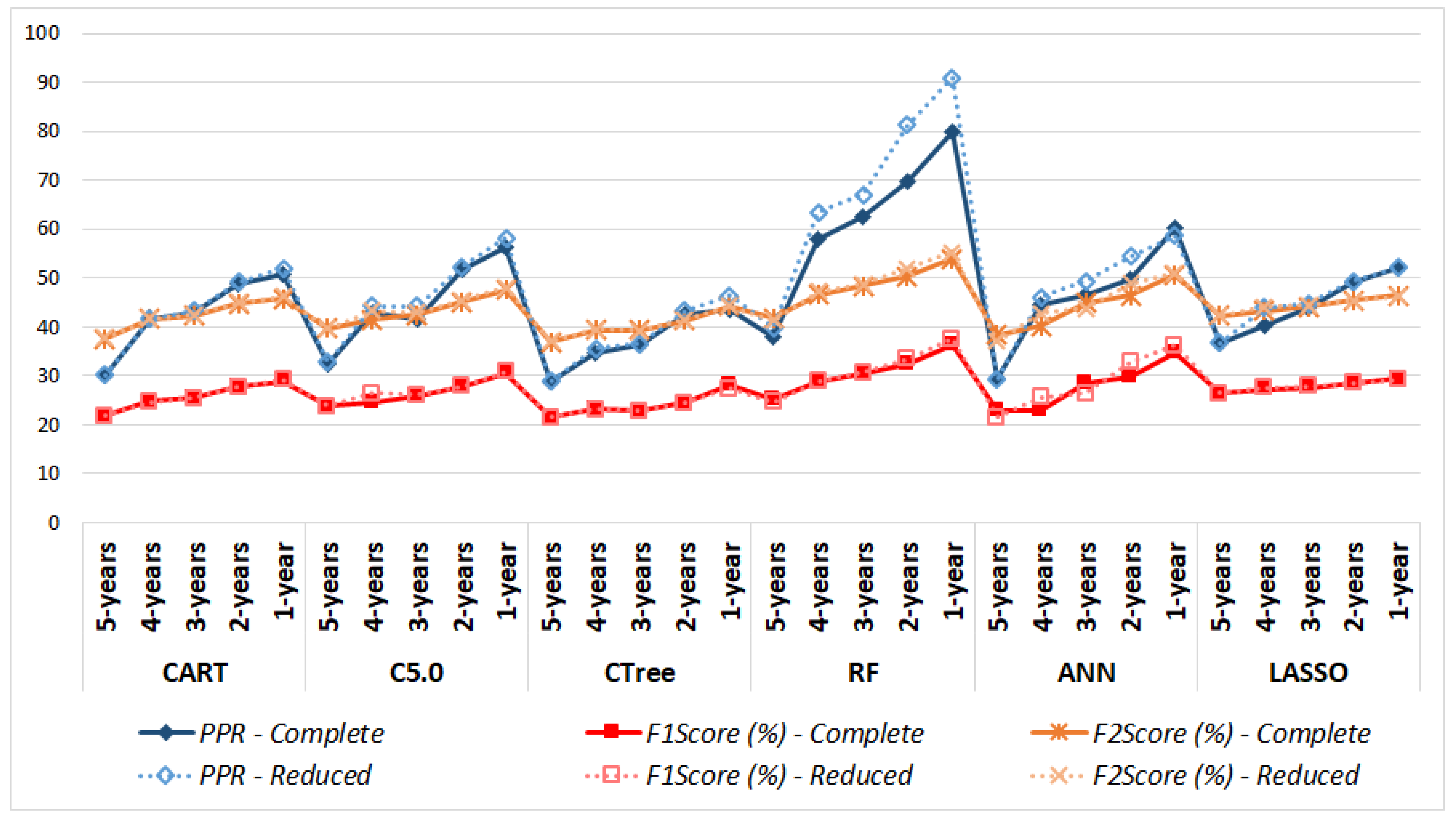
| Model | Dataset | PPR | F1Score (%) | F2Score (%) | SE (%) | SP (%) | PPV (%) | NPV (%) |
|---|---|---|---|---|---|---|---|---|
| CART | Complete | 50.6 | 28.72 | 45.69 | 75.34 | 95.25 | 17.75 | 99.65 |
| Reduced | 51.92 | 29.22 | 46.21 | 75.43 | 95.37 | 18.12 | 99.65 | |
| C5.0 | Complete | 56.31 | 30.31 | 47.48 | 76.32 | 95.55 | 18.91 | 99.66 |
| Reduced | 58.12 | 30.84 | 48.05 | 76.55 | 95.65 | 19.31 | 99.67 | |
| CTree | Complete | 43.68 | 28.12 | 44.28 | 71.8 | 95.39 | 17.48 | 99.6 |
| Reduced | 46.33 | 27.45 | 44.2 | 74.54 | 94.99 | 16.82 | 99.64 | |
| RF | Complete | 79.99 | 36.48 | 53.85 | 78.87 | 96.55 | 23.73 | 99.7 |
| Reduced | 91 | 37.52 | 55.31 | 80.87 | 96.6 | 24.43 | 99.73 | |
| ANN | Complete | 60.09 | 34.7 | 50.63 | 72.98 | 96.63 | 22.76 | 99.62 |
| Reduced | 58.72 | 36.21 | 51.05 | 70.22 | 97.04 | 24.4 | 99.58 | |
| LASSO | Complete | 51.96 | 29.5 | 46.4 | 75.12 | 95.46 | 18.35 | 99.65 |
| Reduced | 52.18 | 29.26 | 46.26 | 75.52 | 95.37 | 18.14 | 99.65 |
| Input Features | Description |
|---|---|
| AGE | Age on 1st January |
| DRUGS_ATC3_A02B | Number of drugs for peptic ulcer and gastro-oesophageal reflux disease |
| DRUGS_ATC3_B01A | Number of antithrombotic agents |
| DRUGS_ATC3_B05B | Number of intravenous solutions |
| DRUGS_ATC3_C01D | Number of vasodilators used in cardiac diseases |
| DRUGS_ATC3_C03C | Number of high-ceiling diuretics |
| DRUGS_ATC3_C03D | Number of potassium-sparing agents |
| DRUGS_ATC3_C07A | Number of beta-blocking agents |
| DRUGS_ATC3_N06A | Number of antidepressant |
| DRUGS_ATC3_V03A | Number of other therapeutic products |
| EX_GROUP_08 | Exemption for disability |
| PERF_GROUP_51 | Number of immunohematology laboratory exams |
Publisher’s Note: MDPI stays neutral with regard to jurisdictional claims in published maps and institutional affiliations. |
© 2020 by the authors. Licensee MDPI, Basel, Switzerland. This article is an open access article distributed under the terms and conditions of the Creative Commons Attribution (CC BY) license (http://creativecommons.org/licenses/by/4.0/).
Share and Cite
Panicacci, S.; Donati, M.; Profili, F.; Francesconi, P.; Fanucci, L. Trading-Off Machine Learning Algorithms towards Data-Driven Administrative-Socio-Economic Population Health Management. Computers 2021, 10, 4. https://0-doi-org.brum.beds.ac.uk/10.3390/computers10010004
Panicacci S, Donati M, Profili F, Francesconi P, Fanucci L. Trading-Off Machine Learning Algorithms towards Data-Driven Administrative-Socio-Economic Population Health Management. Computers. 2021; 10(1):4. https://0-doi-org.brum.beds.ac.uk/10.3390/computers10010004
Chicago/Turabian StylePanicacci, Silvia, Massimiliano Donati, Francesco Profili, Paolo Francesconi, and Luca Fanucci. 2021. "Trading-Off Machine Learning Algorithms towards Data-Driven Administrative-Socio-Economic Population Health Management" Computers 10, no. 1: 4. https://0-doi-org.brum.beds.ac.uk/10.3390/computers10010004