Black-Hole Optimization Applied to the Parametric Estimation in Distribution Transformers Considering Voltage and Current Measures

Abstract

The problem of parametric estimation in single-phase transformers is addressed in this research from the point of view of metaheuristic optimization. The parameters of interest are the series resistance and reactance as well as the magnetization resistance and reactance. To obtain these parameters considering only the voltage and the currents measured in the terminals of the transformer, a nonlinear optimization model that deals with the minimization of the mean square error among the measured and calculated voltage and current variables is formulated. The nonlinear programming model is solved through the implementation of a simple but efficient metaheuristic optimization technique known as the black-hole optimizer. Numerical simulations demonstrate that the proposed optimization method allows for the reduction in the estimation error among the measured and calculated variables when compared with methods that are well established in the literature such as particle swarm optimization and genetic algorithms, among others. All the simulations were carried out in the MATLAB programming environment.

1. Introduction

Electrical transformers are essential devices in the whole electric sector since these devices help with interconnected generation and demand points through transmission lines by increasing the voltage levels from medium-to-high voltage levels [1]. When the transmission lines arrive at the subtramission and distribution substations, the voltage magnitude is again reduced to medium voltage levels to guarantee a secure electricity distribution service [2]; finally, at the load connection points, the voltage is reduced from medium-to-low voltage magnitudes in the final distribution stage [3]. Since the electrical transformers in the transmission and distribution sectors of the electricity service are vitally important, these devices play an important role in the dynamic and static behavior of the whole power system. In the case of static behavior of the grid, one of the main aspects that must be studied corresponds to the number of power losses of the distribution system, since these are an indicator of the grid efficiency, especially in the distribution sector where power losses can vary from 6% to 18% [4], and the transformers can have more than 60% of the total power losses caused mainly by low loadability levels [2]. However, to know the percentage of power losses with a high level of precision, participation of the transformers in the distribution sector is required to reveal the electrical parameters of the transformers. This is not an easy task, since these vary with respect to the nominal values which are influenced by the time of usage, level of loadability, and the weather conditions, among other factors.

Some classical approaches to obtain the electrical parameters of a transformer include laboratory tests such as short-circuit and open-circuit proofs; however, these tests are only possible with transformers that are not being used in the grid, since these tests imply the disconnection of the users to move the transformer from the load point to the laboratory site. This practice is not recommended, as distribution systems can have hundreds of transformers, which implies high expenses as well as affectation of the reliability indexes [5].

To have correct parameters in transformers along distribution test feeders is fundamental for distribution companies, since these parameters help to improve their grid models in order to propose maintaining planes as a function of the grid performance indicators, such as energy losses or transformer loadabilities and efficiencies [6]. To estimate the electrical parameters in transformers without laboratory tests, the literature has proposed multiple approaches that use voltage and current measures to feed an optimization model that determines the best combination of these parameters to reduce the mean square error between the calculated and measured voltages and currents [5]. Some of these literature reports are summarized in

Table 1. Main approaches reported in the specialized literature.

Algorithm	Title	Date
Least Squares	The use of the Least Squares Method to estimate the model parameters of a transformer [7]	September 2009
Bacterial foraging	Parameter estimation of single-phase core type transformer using bacterial foraging algorithm [8]	June 2010
Genetic algorithm	Transformer parameters estimation from nameplate data using evolutionary programming techniques [9]	October 2014
Imperialist competitive	Estimation of transformer parameters from nameplate data by imperialist competitive and gravitational search algorithms [10]	October 2016
Gravitational search	Estimation of transformer parameters from nameplate data by imperialist competitive and gravitational search algorithms [10]	October 2016
Particle swarm optimization	Estimation of equivalent circuit parameters of transformer and induction motor using particle swarm optimization [11]	December 2016
Artificial bee colony	Multi-objective artificial bee colony algorithm to estimate transformer equivalent circuits parameters [12]	November 2017
Chaotic optimization	Estimation of equivalent circuit parameters of single-phase transformer by using chaotic optimization approach [13]	April 2019
Coyote optimization	Parameter estimation of electric power transformers using coyote optimization algorithm with experimental verification [6]	March 2020
Non lineal programming	Parameter estimation in singe-phase transformers employing voltage and current measures [5]	May 2020
Jellyfish Search	Parameter estimation of single-phase transformer using jellyfish search optimizer algorithm [14]	July 2021

.

The main characteristics of the optimization methods listed in Table 1 for solving the parametric estimation in single-phase transformers are as follows:

✓

All of the optimization methods are all from the family of combinatorial optimization approaches, except the work reported in [5] where a large-scale nonlinear solver in the GAMS software was used to solve the model; however, metaheuristic optimization techniques are preferred, since these allow for dealing with the non-convexities of the problem while maintaining the solution space feasible, being implementable in multiple programming languages.

✓

The preferred objective function corresponds to the minimization of the mean square error between the measured and calculated voltages and currents, since this objective function allows for identifying sensitivities among the parameters of the transformers with the main advantage that the transformer is represented using a black-box model, which is internally represented through Kirchoff’s laws.

✓

The main advantage of the metaheuristic optimizers corresponds to their ease of implementation and their low processing times since they only take a few minutes to evaluate a million parameter combinations and possess the ability to explore the whole solution space and exploit some promissory solution regions.

Based on the revision of the state-of-the-art about parametric estimation in transformers, this research identifies the possibility of implementing a new combinatorial optimizer known in the scientific literature as the black-hole optimizer (BHO); this method has not been applied to the problem of parametric estimation in single-phase transformers. The main advantage of this algorithm corresponds to the simple but efficient rules for exploring and exploiting the solution space, which requires the adjusting of only a few parameters.

The main contributions of this research are summarized as follows:

✓

The application of BHO to the parametric estimation in single-phase transformers minimizes the mean square error between the measured and calculated current and voltage variable, with the main advantage that BHO finds minimum errors between the measured and calculated voltage and current variables when compared with classical optimization methods, such as the genetic algorithms, the imperialist competitive algorithm, the particle swarm optimizer, and the gravitational search algorithm.

✓

The reduced computational requirements for the implementation of BHO since the solution of the optimization problem takes about 111.30 s per test system. This is due to its simple evolution rules and the global exploration and exploitation properties of this optimizer, which helps to identify promissory solution regions in a few iterations.

It is worth mentioning that the application of the BHO approach to the problem of parametric estimation in single-phase transformers assumes that the measurements taken in the transformer sizes have been carefully revised and filtered; in addition, the proposed optimization model does not consider additional losses in the transformers due to material deterioration or induced currents in the transformer’s metallic components or three-phase connections. On the other hand, the evaluation of the methodology only covers the fundamental frequency analysis based on the main reports of the specialized literature that accepts the optimization model by considering only the fundamental frequency component to define the electrical parameters of the transformer. Note that these aspects are out of this research’s scope; however, some of these can be considered in future works.

An additional important fact of our research is that we only considers single-phase transformers in the analysis. We selected this type of transformer for two main reasons: (i) in the Colombian context, the vast majority of transformers in medium voltage levels are with single-phase connection with voltages among the primary side in the order of 11 kV to 13.8 kV, which helps with providing electrical service to end users with magnitudes of 120 V or 240 V, depending on the client needs in the secondary side; (ii) most of the research in the literature focus on single-phase transformers, which implies that most of the combinatorial methodologies that are used in this research as comparative methods have previously been validated with high-quality publications.

The remainder of this paper is structured as follows: Section 2 presents the transformer model and the optimization model development; Section 3 presents the main characteristics associated with the implementation of BHO to any optimization problem; Section 4 presents the application of the BHO approach to solve the optimization model defined by Equations (1)–(11); Section 5 presents the implementation of the proposed optimizer to three test systems composed of transformers with nominal powers of 4 kVA, 10 kVA, and 15 kVA, respectively, with their complete analysis and discussions; finally, in Section 6, the main concluding remarks are drawn.

2. Equivalent Transformer Circuit and Optimization Model

The representation of an electrical distribution transformer with an electric circuit depends on the depth of the study [1]; however, two alternatives for representing transformers are widely accepted in the current literature, namely, (i) a circuit equivalent with a magnetization branch in parallel with the voltage source [1]; (ii) the model T of the transformer, i.e., the magnetization branch in the middle in of the series branches [13]. Here, we adopt the second model since this presents a better approximation of the electrical performance of the transformer regarding steady-state studies. 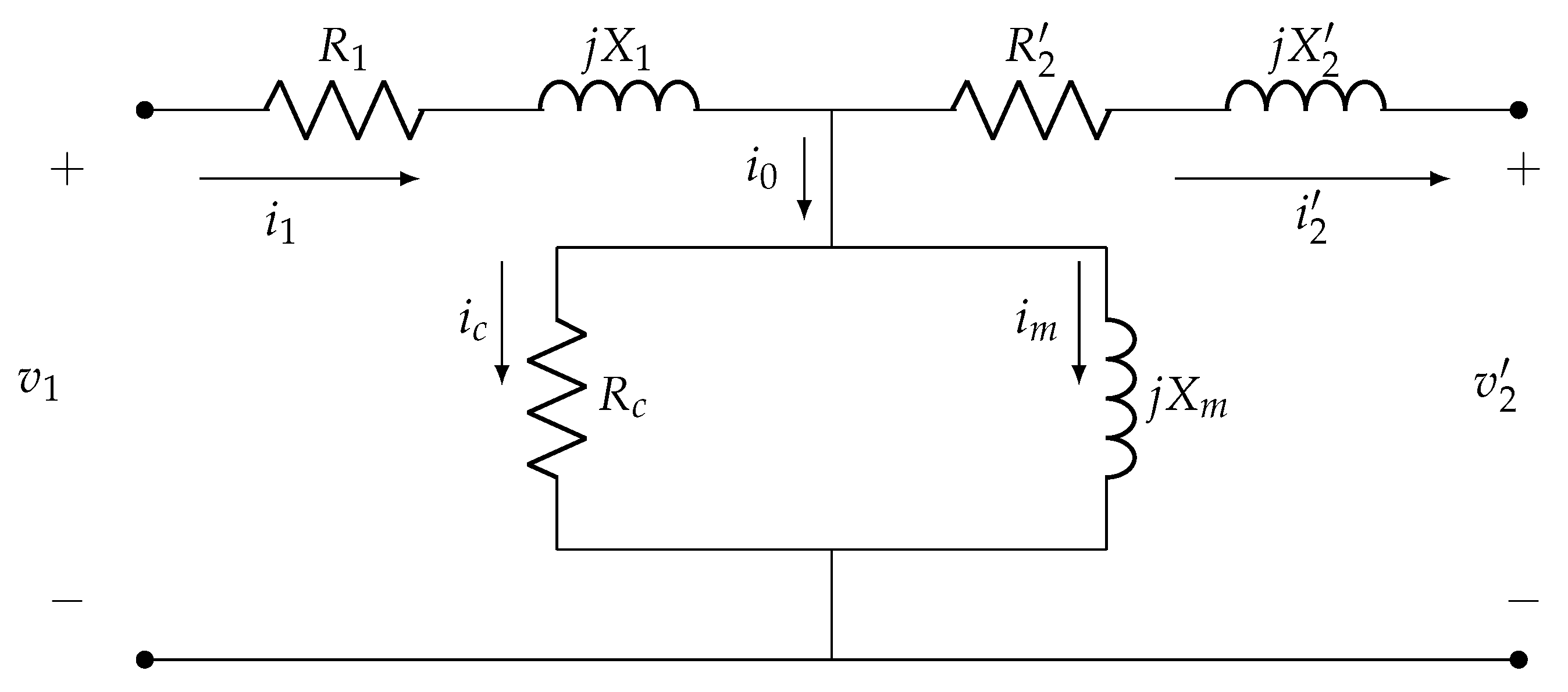Figure 1 depicts the equivalent circuit of the transformer analysed in this research.

From the electrical circuit presented in Figure 1, we can observe the following: $R_1$ and $X_1$ represents the resistance and reactance parameters of the primary side of the transformer, while $R_2^{\prime }$ and $X_2^{\prime }$ correspond to the resistance and reactance parameters in the secondary side of the transformer referred to the primary side; $X_m$ and $R_c$ are the magnetization reactance and resistance that models the energy dissipation effects in the core of the transformer; $R_{\mathrm{load}}$ represents the equivalent resistance associated with the load connected to the transformer in its secondary side. Note that the electrical variables in Figure 1 are the primary current $i_1$ and the secondary current referred to the primary side $i_2^{\prime }$ as well as the secondary voltage in the primary side, i.e., $v_2^{\prime }$. It is important to mention that the primary voltage $v_1$ is considered as an input, which implies that it is a parameter for the problem parametric estimation in transformers [5].

To obtain the equivalent impedance of the transformers at the input terminals, the equivalent resistance load is connected in the $V_2^{\prime }$ terminals is considered, which produces the following equivalent impedance.

$$Z=Z_1+\frac{Z_0\left(Z_2^{\prime }+R_{\mathrm{load}}\right)}{Z_0+Z_2^{\prime }+R_{\mathrm{load}}^{\prime }}$$

(1)

where $Z_1=R_1+j{X}_1$ represents the primary equivalent impedance, $Z_2^{\prime }=R_2^{\prime }+j{X}_2^{\prime }$ corresponds to the secondary impedance referred to the primary side, and $Z_0=j\frac{R_c{X}_m}{R_c+j{X}_m}$ is the magnetization impedance.

Once the equivalent transformer impedance is calculated, then, the primary current can be calculated as follows:

$$i_1=\frac{v_1}{Z}.$$

(2)

Now, using the divisor current concept, the secondary current referred to the primary side is defined as presented below:

$$i_2^{\prime }=\frac{Z_0}{Z_0+Z_2^{\prime }+R_{\mathrm{load}}}\frac{v_1}{Z},$$

(3)

Finally, the value of the secondary voltage referred to the primary side is calculated as follows:

$$V_2^{\prime }=R_{\mathrm{load}}{I}_2^{\prime }.$$

(4)

To formulate the problem of the parametric estimation in single-phase transformers, a quadratic function that determines the average error between the measured and calculated electric variables is considered, which takes the following form:

$$\begin{array}{c}\hfill minz=\frac{1}{2}\left({\left(\frac{{\overline{I}}_1-i_1}{{\overline{I}}_1^2}\right)}^2+{\left(\frac{{\overline{I}}_2^{\prime }-i_2^{\prime }}{{\overline{I}}_2^{\prime }}\right)}^2+{\left(\frac{{\overline{V}}_2^{\prime }-v_2^{\prime }}{{\overline{V}}_2^{\prime }}\right)}^2\right),\end{array}$$

(5)

where z corresponds to the average mean square error. It is important to highlight that ${\overline{I}}_1$, ${\overline{I}}_2^{\prime }$ and ${\overline{V}}_2^{\prime }$ correspond to the primary and secondary measured currents as well as the secondary measured voltage, respectively.

The set of constraints of the parametric estimation problems in transformers is complete with the equality constraints (1)–(4) and the upper and lower bounds of the decision variables presented below:

$$\begin{array}{c}\hfill R_1^{min}\le R_1\le R_1^{max},\end{array}$$

(6)

$$\begin{array}{c}\hfill R_2^{\prime ,min}\le R_2^{\prime }\le R_2^{max,\prime },\end{array}$$

(7)

$$\begin{array}{c}\hfill R_c^{min}\le R_c\le R_c^{max},\end{array}$$

(8)

$$\begin{array}{c}\hfill X_1^{min}\le X_1\le X_1^{max},\end{array}$$

(9)

$$\begin{array}{c}\hfill X_2^{\prime ,min}\le X_2^{\prime }\le X_2^{max,\prime },\end{array}$$

(10)

$$\begin{array}{c}\hfill X_m^{min}\le X_m\le X_c^{max}.\end{array}$$

(11)

where $y^{min}$ and $y_{max}$ represent the minimum and maximum limits of the decision variables.

Remark 1.

The complete optimization model composed for the objective function (5) and the set of constraints (1)–(4) in conjunction with constraints (6)–(11) represents the problem of the parametric estimation problem in single-phase transformers [13]; it has a nonlinear non-convex structure due to the fractions and products among the variables in the calculated voltage and current variables. This situation implies that efficient optimization techniques are required as is the case of the black-hole optimizer presented in this research, which is simple to implement, but is efficient in solving nonlinear continuous optimization problems [15].

3. Black-Hole Optimization Algorithm

The black-hole optimizer (BHO) is a metaheuristic optimization technique from the family of the nature-inspired optimization algorithms [16], which adapt physical behaviors in evolution rules to solve multiple engineering optimization problems [17,18].

The BHO algorithm works by formulating the interaction among stars and black holes in the center of galaxies with some simple mathematical rules that allows exploring and exploiting the solution space in engineering problems; its main characteristic is that it is a population-based optimization algorithm, where the stars are the individuals in the population and the black hole represents the best current solution [15].

The main steps in the implementation of the BHO algorithm are described below.

3.1. Stars’ Birth

As with most population-based optimization algorithms, the BH optimizer starts its exploration and exploitation of the solution space with an initial population (stars uniformly distributed along the solution space), which is randomly generated. The initial population is set with $n_i$ individuals on it, where each one of the rows represents a potential solution of the problem under study [19]. Note that in the case of the parametric estimation in single-phase transformers, the dimension of the initial population is a matrix with $n_i$ rows and $N_v$ columns, where $n_v$ represents the number of variables, i.e., 6 in our study case.

The initial population is generated with the following rule:

$$\begin{array}{c}\hfill P_t=x^{min}o\left(n_i,n_v\right)+\left(x^{max}-x^{min}\right)r\left(n_i,n_v\right),\end{array}$$

(12)

where $P_t$ represents the initial population when $t=0$, being t the iterative counter; $O\left(n_i,n_v\right)$ is a matrix filled by ones with $n_i$ rows and $n_v$ columns; $r\left(n_i,n_v\right)$ is a random matrix filled by numbers between 0 and 1 with a normal distribution; in addition, $x^{min}$ and $x^{max}$ are vectors with dimensions $1\times n_v$ that contains all the lower and upper bounds of the decision variables, i.e.,

$$\begin{array}{c}\hfill x^{min}={\left[R_1^{min}{R}_2^{min}{R}_c^{min}{X}_1^{min}{X}_2^{min}{X}_m^{min}\right]}^T,\\ \hfill x^{max}={\left[R_1^{max}{R}_2^{max}{R}_c^{max}{X}_1^{max}{X}_2^{max}{X}_m^{max}\right]}^T.\end{array}$$

Note that the main advantage of the generation of the initial population, i.e., $P_t$ with Equation (12), is that it generates feasible solutions, since each individual is inside of its lower and upper bounds.

3.2. Stars’ Movement

Owing to the intense gravitational force that black holes have, all the stars in the neighborhood of a black hole is affected, as can be observed in Figure 2.

In this sense, the gravitational force of the black hole makes the stars have dynamic behavior as a function of their relative position with respect to the black hole [15]. To formulate this behavior of the stars, their next position can be formulated as follows:

$$P_{t+1}^i=P_t^i+\left(P{t}^{BH}-P_t^i\right)r\left(1,n_v\right);i=1,2,\dots ,n_i,$$

(13)

where $P_t^{BH}$ represents the relative position of the black hole, i.e., the best current solution in the population, and $P_{t+1}^i$ represents the relative position of the ith star after its interaction with the black hole. Note that during the star’ movements, the position of the black hole remains unaltered.

Remark 2.

To preserve the feasibility of the solution space once the stars interact with the black hole, each one of the individuals $P_{t+1}^i$ is revised to ensure that it is contained between its upper and lower bounds using the following rule:

$$\begin{array}{c}\hfill P_{t+1}^{ij}=\left\{\begin{array}{cccc}{P}_{t+1}^{ij}& if& x_j^{min}\le P_{t+1}^i\le x_j^{max}& \left[\begin{array}{c}i=1,2,...,n_i\\ j=1,2,...,n_v\end{array}\right]\\ x_j^{min}+\left(x_j^{max}-x_j^{min}\right)r\left(1,1\right)& if& P_{t+1}^i<x_j^{min}\left|\right|P_{t+1}^i>x_j^{max}& \left[\begin{array}{c}i=1,2,...,n_i\\ j=1,2,...,n_v\end{array}\right]\end{array}\right.\end{array}$$

(14)

3.3. Black-Hole Updating

Once the descending population is generated, i.e., $P_{t+1}$, the position of the black hole can be modified if one of the stars in the current population has a better objective function value. To verify the change in the position of the black-hole, the following rule is applied:

$$\begin{array}{c}\hfill P_{t+1}^{BH}=\left\{\begin{array}{cccc}{P}_t^{BH}& \mathrm{if}& z_f\left(P_t^{BH}\right)<z_f\left(P_{t+1}^i\right)& i=1,2,...,n_i\\ P_{t+1}^i& \mathrm{if}& z_f\left(P_t^{BH}\right)>z_f\left(P_{t+1}^i\right)& i=1,2,...,n_i\end{array}\right.\end{array}$$

(15)

where $z_f\left(P_{t+1}^i\right)$ represents the objective function value associated with the $\left(i+1\right)$th individual in the next population.

It is worth mentioning that $z_f$ is calculated by using the objective function formulated in Equation (5) and/or an adaptation of this.

3.4. Star’s Replacing

The main characteristic of BHO is the strong interaction among stars and the black hole. The black hole can absorb or eject a star around its neighborhood (see Figure 2). To emulate this behavior in nature, BHO uses a probability of crossing the horizon of events (point where any object absorbed by a black hole is destroyed). In the case of a star crossing the event’s horizon, this will be replacing a new star randomly generated, ensuring the feasibility of the solution space. The key of this process is the determination of the event’s horizon radius, i.e., $R_{EH}$, which as recommended in [19] and can be calculated as follows:

$$R_{EH}=\frac{z_f\left(P_{t+1}^{BH}\right)}{{\displaystyle \sum _{i=1}^{n_i}{z}_f\left(P_{t+1}^i\right)}},$$

(16)

To determine if an arbitrary star inside of the population cross the horizon of events, the ${\mathrm{norm}}_{l_2}$ is used [19], where it is widely known in the current literature as the Euclidean distance, which is calculated as follows:

$$D_{BH-i}=∥{\displaystyle P_{t+1}^{BH}-P_{t+1}^i}∥,i=1,2,\dots ,n_i$$

(17)

Note that if $R_{EH}<D_{BH-i}$, the $\left(i+1\right)$th star will be absorbed (i.e., destroyed) by the black hole, giving the possibility that a new star born in the solution space. It is worth mentioning that once a star is destroyed, a new one is created to maintain the number of individuals inside of the population constant. An important fact associated with the stars’ birth is regarding the ability of BHO to explore and exploit the solution space in a global manner [20].

3.5. Completion Criteria

To finish the exploration and exploitation of the solution space, BHO uses one of the following completion criteria:

• If the objective function $z_f$ does not vary during $k_{max}$ consecutive iterations, then, the optimization process ends, and the optimal solution of the problem corresponds to the $P_{t+1}^{BH}$.
• If the number of iterations $t_{max}$ is reached, then, the final solution $P_{t+1}^{BH}$ is reported and the optimization process ends.

4. Application of BHO to the Studied Problem

Unlike the classical approach where short-circuit and open-circuit tests are employed to determine the electrical parameters of an electrical distribution transformers in a laboratory [9], the main idea of this research is to determine the parameters of the transformers considering only voltage and current measures taken directly from the location of the transformer without disconnecting its local load.

To applied BHO to the parametric estimation problem in single-phase distribution transformers, here, we adopt a modification of the objective function (5) using an equivalent mean square error with the following form:

$$Z_f={\left({\overline{I}}_1-i_1\right)}^2+{\left({\overline{I}}_2^{\prime }-i_2^{\prime }\right)}^2+{\left(V_2^{\prime }-v_2^{\prime }\right)}^2$$

(18)

Note that the summation in (18) is only possible if all the values are normalized using per-unit representation. The application of BHO to the problem of the parametric estimation in single-phase transformers is presented in Algorithm A1 available in the Appendix A. For more details about the BHO approach, the following references can be consulted: [15,19].

Remark 3.

An important fact previous to the implementation of an optimization strategy to determine the electrical parameters in transformers is associated with the data analysis of the voltage and current measured inputs. These data must be filtered and also normalized to avoid spurious information that can alter the final result of the optimization process.

5. Results and Discussion

This section presents the analysis of the results and their discussion when the proposed BHO is applied to solve the problem of the parametric estimation in single-phase transformers with nominal rates of 4 kVA, 10 kVA, and 15 kVA. The parametric information of these transformers was taken from references [9,10]. Different optimization methods reported in the specialized literature were used as comparative methodologies were considered, which includes particle swarm optimization (PSO) [9], genetic algorithms (GA) [9], imperialist competitive algorithm (ICA) [10], and gravitational search algorithm (GSA) [10]. In addition, to determine the average processing times taken by the proposed BHO to solve the studied optimization problem, three consecutive evaluations are made for each test system. All the numerical implementations were carried out in a personal computer AMD Ryzen 5 3500U processor 2.10 GHz. RAM 8 Gb, with a Windows 10 operating system, single language, 64 bits. In the computational evaluation, we have considered 100 consecutive evaluations of the BH optimizer in order to determine the standard deviation of the objective function and the average processing time per execution.

5.1. First Test System: 4 kVA, 50 Hz, 250/125 V Transformer

This is a low-voltage/low-voltage single-phase transformer with a nominal power transference capability of 4 kVA, operated with 50 Hz, with a voltage relation of 250/125 V. For this transformer, all the measures are assumed with full resistive load, i.e., $R_{\mathrm{load}}=15.625$ Ω [9]. It is worth mentioning that the real values associated with the electrical parameters of this transformer were taken from [9], which are named in

Table 2. Numerical comparison among the parameters in the first test system.

Parameter	${\mathit{R}}_1$ (Ω)	${\mathit{X}}_1$ (Ω)	${\mathit{R}}_2^{\mathit{\prime }}$ (Ω)	${\mathit{X}}_2^{\mathit{\prime }}$ (Ω)	${\mathit{R}}_{\mathit{c}}$ (Ω)	${\mathit{X}}_{\mathit{m}}$ (Ω)	Average Error (%)
Actual [9]	0.4	0.2	0.4	2	1500	750	-
PSO [9]	0.587	0.2554	0.209	1.602	1476	738	-
PSO error (%)	46.750	27.700	47.7500	19.900	1.600	1.600	24.218
GA [9]	0.598	0.226	0.336	1.957	1410	707	-
GA error (%)	49.500	13.0000	16.000	2.150	6.000	5.733	15.397
ICA [10]	0.430	0.202	0.394	2.500	1200.00	700.00	-
ICA error (%)	7.500	1.000	1.500	25.000	20.000	6.667	10.278
GSA [10]	0.425	0.203	0.415	2.399	1426.00	745.30	-
GSA error (%)	6.2500	1.500	3.7500	19.950	4.933	0.627	6.168
BHO	0.4512	0.2492	0.3780	1.7016	1478.7763	684.8906	-
BHO error (%)	12.8199	24.6172	5.4908	14.9163	1.4149	8.6812	11.3234

as the actual data.

Numerical results in Table 2 shows that the lowest mean error is provided by the GSA method with a value of 6.168%, followed by the ICA with a value of $10.278\%$ and in third place is located the proposed BHO with an average error about $11.3234\%$; Note that this error is highly influenced by the errors introduced with the parameters with small magnitudes such as series resistance and inductance parameters. However, when is analyzed the level of precision of the proposed BHO to find the error between the calculated and the measured variables our approach presents the best numerical performance as can be seen in

Table 3. Comparison among measured and calculated variables for the first test system.

Transformer Data	${\mathit{I}}_1$ (A)	${\mathit{I}}_2^{\prime }$ (A)	${\mathit{V}}_2^{\mathit{\prime }}$ (V)	Average Error (%)
Actual (Measured)	15.2825	15.0782	235.5967	-
PSO	15.3153	15.1172	236.2065	-
PSO error (%)	0.2146	0.2587	0.2588	0.2440
GA	15.1714	14.9574	233.7093	-
GA error (%)	0.7270	0.8012	0.8011	0.7764
ICA	15.2449	14.9881	234.1894	-
ICA error (%)	0.2460	0.5976	0.5973	0.4803
GSA	15.2091	14.9893	234.2083	-
GSA error (%)	0.4803	0.5896	0.5893	0.5531
BHO	15.2826	15.0782	235.5967	-
BHO error (%)	0.0007	0.0000	0.0000	0.0002

The value of the fitness function is $2.05\times {10}^{-10}$; Average execution time per evaluation 108.5061 s; The standard deviation value is $4.999\times {10}^{-8}$.

.

Numerical results in Table 3 show that BHO has an average error about $2.0\times {10}^{-4}\%$ among the measured and calculated voltage and current variables, followed by the PSO approach with an average error of $0.2440\%$; which implies that the precision of the proposed approach is at least 1000 times better than the PSO approach.

An important fact observed from the results in Table 2 and Table 3 is that even if BHO is the third best approach when compared each individual parameter, it is the best when the difference among measured variables and calculated variables is analyze, which confirms that the problem of the parametric estimation in single-phase transformers is nonlinear and non-convex and can have multiple local optimums; however, the value of the average error among the measured and calculated variables shows that BHO finds a high-quality local optimum when compared with the remainder optimization techniques. Note that the standard deviation value for this test system is about $4.999\times {10}^{-6}\%$, which demonstrates that BHO finds solutions inside of a small ball at each execution, which confirms its efficiency in solving the studied problem by providing the quasi-optimal solutions at each evaluation.

5.2. Second Test System: 10 kVA, 50 Hz, 500/125 V Transformer

This test system corresponds to a low-voltage/low-voltage transformer with a nominal power transference capability of 10 kVA, operated with 50 Hz, and a voltage relation of 500/125 V [10]. The nominal restive load for this transformer is equivalent to $R_{\mathrm{load}}=25$ Ω.

Table 4. Numerical comparison among the parameters in the second test system.

Parameter	${\mathit{R}}_1$ (Ω)	${\mathit{X}}_1$ (Ω)	${\mathit{R}}_2^{\mathit{\prime }}$ (Ω)	${\mathit{X}}_2^{\mathit{\prime }}$ (Ω)	${\mathit{R}}_{\mathit{c}}$ (Ω)	${\mathit{X}}_{\mathit{m}}$ (Ω)	Average Error (%)
Actual [9]	0.9	0.94	1.6	0.44	700	250	-
PSO [9]	0.811	0.8608	1.678	0.7540	713	314.2	-
PSO error (%)	9.8889	8.4255	4.8750	71.3636	1.8571	25.6800	20.3484
GA [9]	1.025	0.8	1.507	0.493	651.5	204.4	-
GA error (%)	13.8889	14.8936	5.8125	12.0455	6.9286	18.2400	11.9682
ICA [10]	0.8	0.8	1.5	0.4259	692.48	255	-
ICA error (%)	11.1111	14.8936	6.2500	3.2045	1.0743	2.0000	6.4223
GSA [10]	0.8001	0.8119	1.5004	0.4236	695.54	251.35	-
GSA error (%)	11.1000	13.6277	6.2250	3.7273	0.6371	0.5400	5.9762
BHO	0.943	1.034	1.535	0.624	698.676	263.512	-
BHO error (%)	4.7778	10.0000	4.0625	41.8182	0.1891	5.4048	11.0421

presents the comparison among the actual (i.e., real) data for each optimization approach.

It is worth mentioning that as has happened for the the first test system, in this simulation case, the GSA approach has the lowest average error per parameter with a value of $5.9762\%$, followed by the ICA with a value of $6.4223\%$, and in the third place is the proposed BHO with an error about $11.0421\%$; however, when the error is observed among the measured and calculated variables (see

Table 5. Comparison among measured and calculated variables for the second test system.

Transformer Data	${\mathit{I}}_1$ (A)	${\mathit{I}}_2^{\prime }$ (A)	${\mathit{V}}_2^{\mathit{\prime }}$ (V)	Average Error (%)
Actual	18.8877	18.0722	451.8047	-
PSO	18.8719	18.0906	452.2639	-
PSO error (%)	0.0837	0.1018	0.1016	0.0957
GA	18.9683	18.0472	451.1802	-
GA error (%)	0.4267	0.1383	0.1382	0.2344
ICA	19.0427	18.2217	455.5431	-
ICA error (%)	0.8206	0.8272	0.8274	0.8251
GSA	19.0405	18.2196	455.4897	-
GSA error (%)	0.8090	0.8156	0.8156	0.8134
BHO	18.8877	18.0722	451.8047	-
BHO error (%)	0.0000	0.0000	0.0000	0.0000

The value of the fitness function is $3.4064\times {10}^{-10}$; Average execution time per evaluation 116.0146 s; The standard deviation value is $2.1398\times {10}^{-9}$.

), BHO is the best methodology to find a solution.

Results in Table 5 demonstrate that BHO is the best optimization method regarding the minimization of the error among the measured and calculated voltage and current variables with an error of $0.0\%$, which implies that the number of decimals considered in the measurement the coincidence with the calculated variables is perfect. When the objective function value is observed, the BHO approach reaches a value lower than $1.44\times {10}^{-10}$, which can be considered as zero for any practical implementation purposes, which is confirmed by a standard deviation of $2.1398\times {10}^{-7}\%$.

5.3. Third Test System: 15 kVA, 50 Hz, 2400/240 V Transformer

The third transformer corresponds to a medium-voltage/low voltage transformer with a nominal power transference capability of 15 kVA, which is operated with 50 Hz, and a voltage relation of 2400/240 V [10]. The nominal equivalent resistive load for this transformer is $R_{\mathrm{load}}=384$ Ω. Comparative results among parameters are reported in

Table 6. Numerical comparison among the parameters in the third test system.

Parameter	${\mathit{R}}_1$ (Ω)	${\mathit{X}}_1$ (Ω)	${\mathit{R}}_2^{\mathit{\prime }}$ (Ω)	${\mathit{X}}_2^{\mathit{\prime }}$ (Ω)	${\mathit{R}}_{\mathit{c}}$ (Ω)	${\mathit{X}}_{\mathit{m}}$ (Ω)	Average Error (%)
Actual [9]	2.45	3.14	2	2.2294	105000	9106	-
PSO [9]	2.25	4.082	2.2	1.8526	99517	9009	-
PSO error (%)	8.1633	30.0000	10.0000	16.9014	5.2219	1.0652	11.8920
GA [9]	2.76	3.414	1.68	1.846	97001	8951	-
GA error (%)	12.6531	8.7261	16.0000	17.1975	7.6181	1.7022	10.6495
ICA [10]	2	3	1.80	2	120000	9200	-
ICA error (%)	18.3673	4.4586	10.0000	10.2898	14.2857	1.0323	9.7390
GSA [10]	2	3.11	1.81	2.26	104281	9094.87	-
GSA error (%)	18.3673	0.9554	9.5000	1.3726	0.6848	0.1222	5.1671
BHO	2.4268	3.915	1.9807	2.670	103891.266	9473.402	-
BHO error (%)	0.9469	24.6815	0.9650	19.7632	1.0559	4.0347	8.5745

for the literature reports and the proposed BHO with respect to the actual data.

The comparison between the average error with respect to the transformer parameters shows once again that the GSA is the better optimization approach with a value of $5.1671\%$; however, for this test system, the proposed BHO falls in the second place with an average error of $8.5745\%$, followed by the third place by the ICA with a value of $9.7390\%$. Notwithstanding, when

Table 7. Comparison among measured and calculated variables for the third test system.

Transformer Data	${\mathit{I}}_1$ (A)	${\mathit{I}}_2^{\prime }$ (A)	${\mathit{V}}_2^{\mathit{\prime }}$ (V)	Average Error (%)
Actual	6.2053	6.1756	2371.4	-
PSO	6.2056	6.1748	2371.1	-
PSO error (%)	0.0048	0.0130	0.0127	0.0101
GA	6.2070	6.1755	2371.4	-
GA error (%)	0.0274	0.0016	0.0000	0.0097
ICA	6.2128	6.1861	2375.5	-
ICA error (%)	0.1209	0.1700	0.1729	0.1546
GSA	6.2157	6.1858	2375.3	-
GSA error (%)	0.1676	0.1652	0.1645	0.1657
BHO	6.2053	6.1755	2371.4	-
BHO error (%)	0.0000	0.0016	0.0000	0.0005

The value of the fitness function is $6.5670\times {10}^{-9}$; Average execution time per evaluation 109.3800 s; The standard deviation value is $5.5668\times {10}^{-10}$.

is observed, it is possible to confirm that as had happened in the previous test systems as well, the proposed BHO reaches the minimum error among the measured and calculated variables with an error of $5\times {10}^{-4}$; this is at least 19 times better than the GA, which has an average error of $9.70\times {10}^{-3}$. In addition, the effectiveness of the BH optimizer to obtain quasi-optimal solutions at each evaluation is confirmed with a standard deviation value of about $5.5668\times {10}^{-8}\%$ that allows ensuring that all the solutions are contained inside a ball with a pretty small radius.

5.4. Complementary Analysis

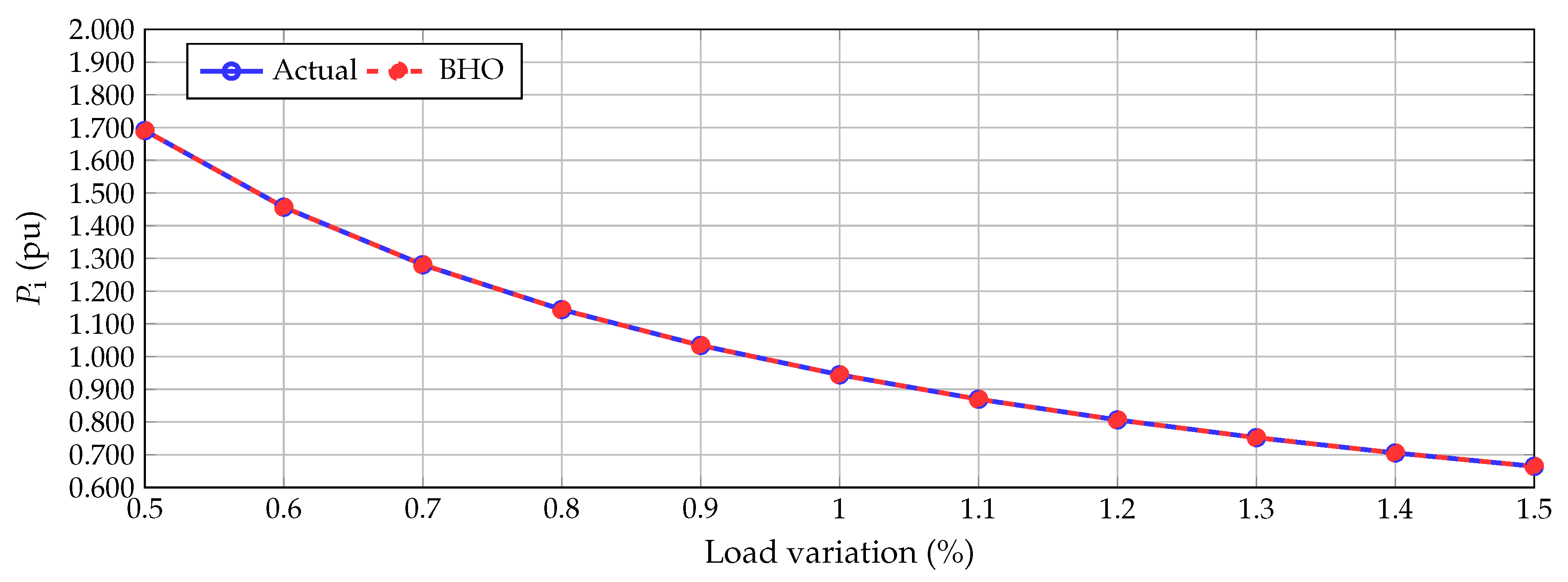
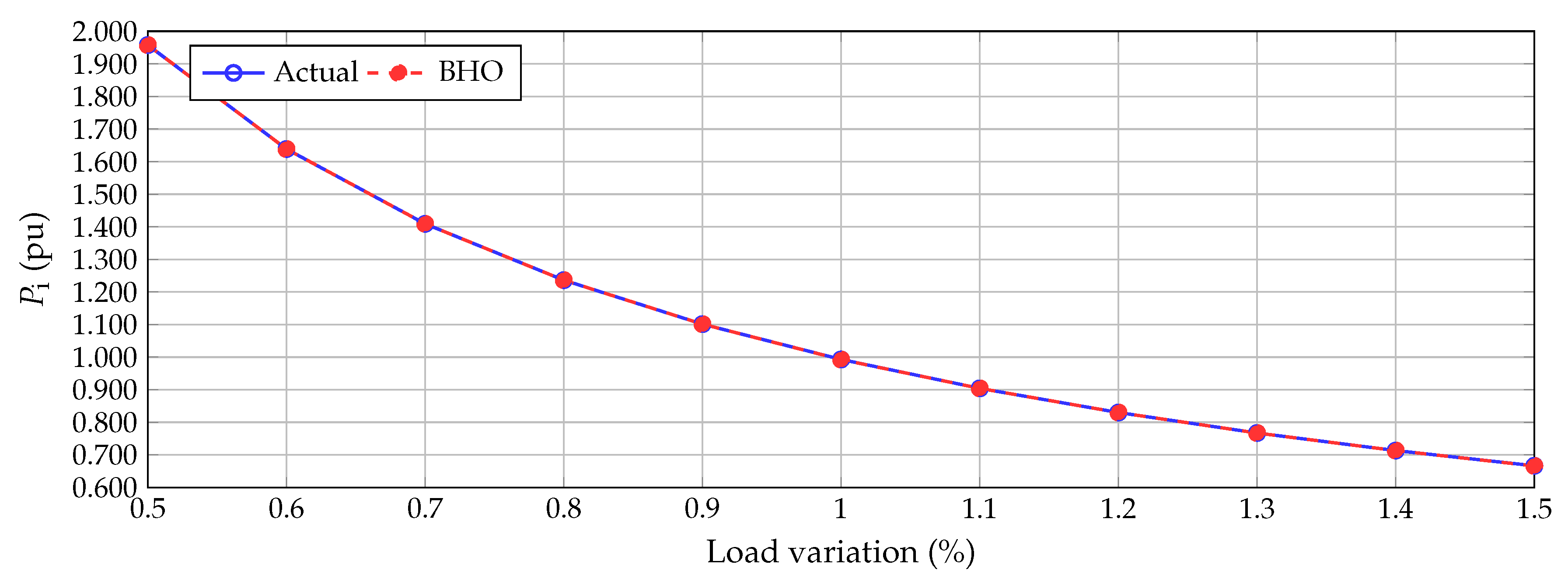
This section shows the effectiveness of the proposed estimation method for the electrical parameters of single-phase transformers with primary and secondary windings and the magnetization branch. To demonstrate that the actual parameters of the transformer and the estimation provided by our proposed BHO have negligible errors, we vary the constant resistive load in its terminals from 50% to 150% of its nominal value, and we plot the per-unit power input calculated with the real and estimated transformer parameters, using the following formula:

$$P_{\mathrm{i}}=\frac{\mathrm{Real}\left\{v_1{i}_1^{★}\right\}}{S_{\mathrm{n}}},$$

(19)

where $P_{\mathrm{i}}$ represents the input power in the primary terminals of the transformer, and $S_{\mathrm{n}}$ is defined as the nominal power rate of the transformer.

The behavior of the input power for each of the test systems is depicted in Figure 3, Figure 4 and Figure 5, respectively.

From these plots, we can observe the following:

✓

An equivalent resistance value of 50% of its nominal value implies different power inputs at each transformer, these being 1.7713 pu, 1.6908 pu, and 1.9578 pu, for the first, second, and third transformer, respectively. This behavior is explained in the power input of any transformer, since if the input voltage is constant, and the resistance load is reduced, then, the amount of current absorbed by the transformer increases.

✓

The minimum power input for each transformer is caused when the equivalent resistive load is 150% of its nominal value, in this case, the first, second, and third transformers consume 0.6539 pu, 0.6645 pu, and 0.6660 pu, respectively. These values imply that the loadabilities of these transformers are between 65% and 67%. Note that the effect of equivalent loads higher than 100% implies that the consumed currents are reduced (Ohm’s law), which is directly connected with the reduction in the power input.

✓

The most important fact in Figure 3, Figure 4 and Figure 5 is that the estimated parameters and the actual data provide overlapped curves, which implies that from the circuital point of view (e.g., voltage, current and power calculations), the BHO approach is an adequate method to solve the problem of parametric estimation in single-phase transformers with errors lower than $1\times {10}^{-3}\%$.

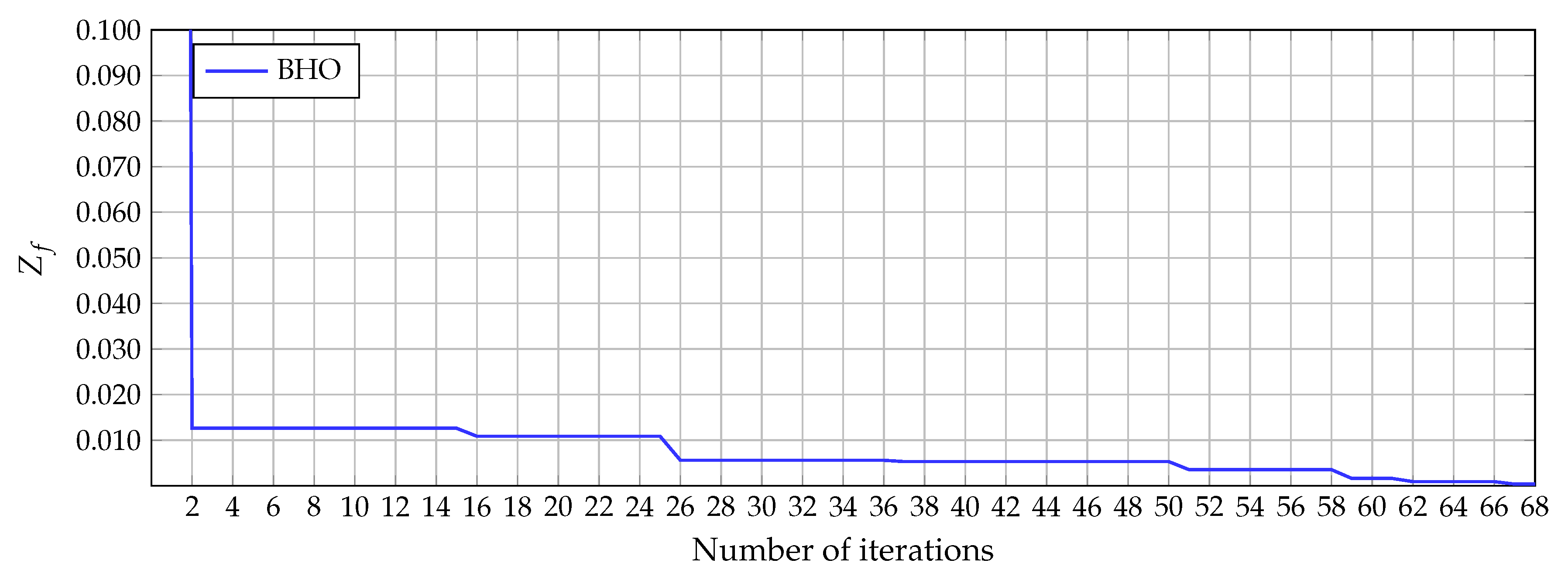
On the other hand, Figure 6 presents the numerical behaviour of the objective function when the proposed BHO is applied to estimate the electric parameters of the third transformer.

From Figure 6, we can note that the objective function is lower than $0.020$ after Iteration 2, which shows that the algorithm rapidly converges to an adequate function value lower than $6.5670\times {10}^{-9}$ in this test system.

After the application of BHO to determine all the electrical parameters of single-phase transformers considering voltage and current measures, we observe the following positive aspects of this algorithm: (i) the effectiveness of the exploration and exploitation of the solution space with simple evolution rules that allows us to identify promissory solution regions at the beginning of the searching process to be exploited when the iteration procedure advances; (ii) the easy adjusting process for the BHO parameters, since it only requires the definition of the population size and the number of iterations. The most important factor in this tuning is to find an adequate trade-off between the reduction in the objective function and the total processing time.

It is worth mentioning that after observing the final results regarding each particular parameter of the transformer and the final objective function value provided by BHO, there exists a low correlation among these variables since higher differences among the actual and calculated parameters do not imply high values in the objective function. This low correlation is explained as follows:

• The nature of the optimization model is indeed nonlinear and non-convex, which implies that there can exist infinite solutions with similar objective functions dispersed along with the solution space, as reported by the different methodologies in the comparative reports.
• The effect of the magnetization branch in the total injected current is minimum since this branch is in the order of kΩ, which implies that values less than 10% of the current flow though of it. This implies that higher variations on these parameters have insignificant effects of the final calculated currents.
• The equivalent impedance of the transformer is dominated by the load resistance, which implies that the equivalent effect of the parameters of the transformers are reduced when the complete circuit is analyzed; this implies that variations in these parameters does not drastically influence the final objective function value.

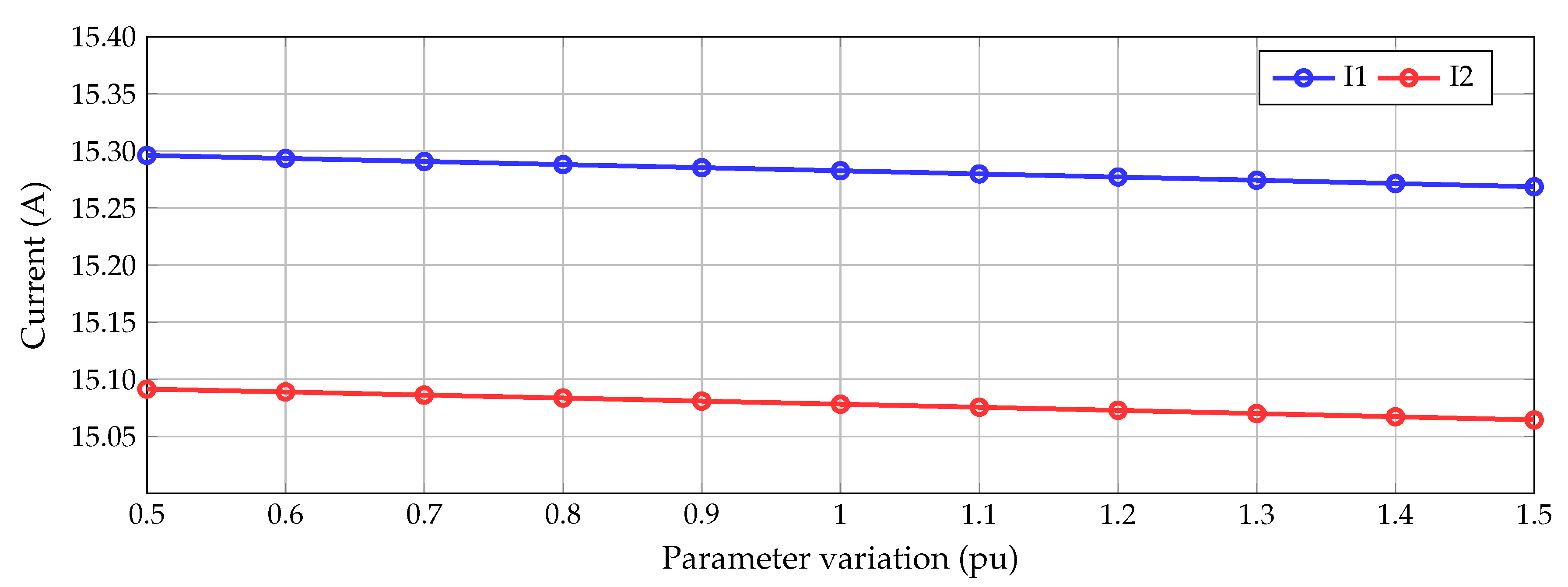
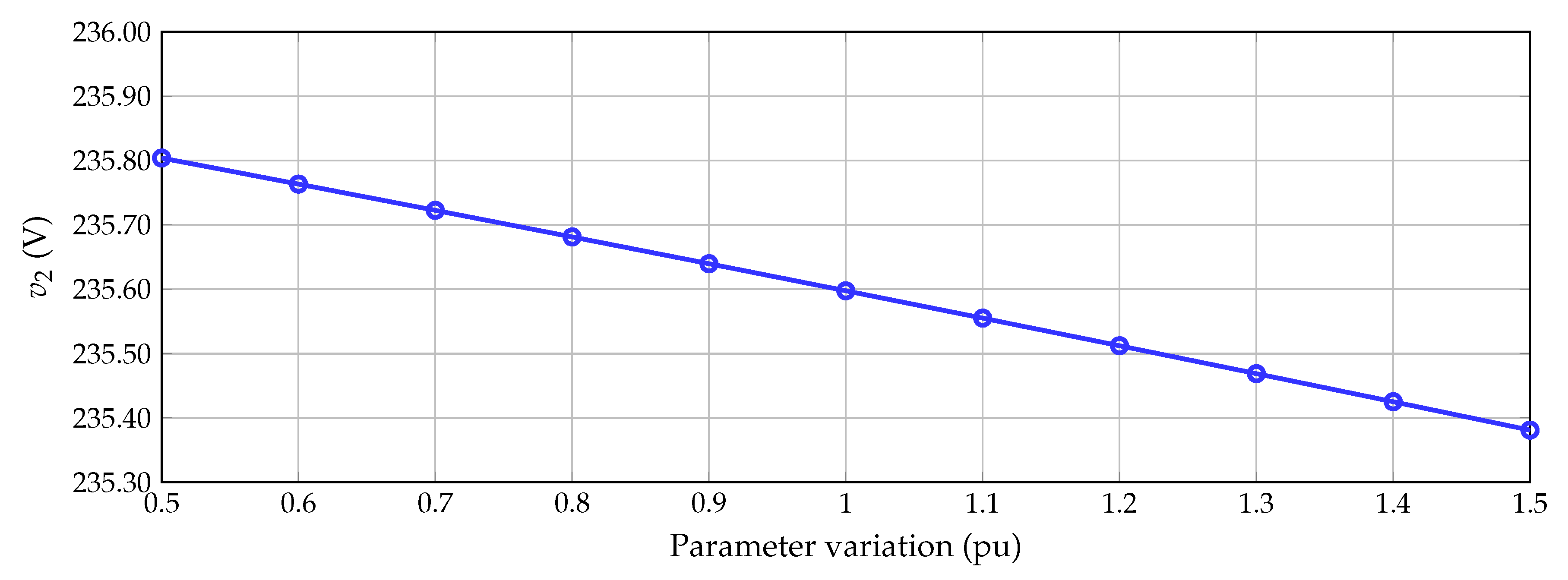
To demonstrated that large differences in the transformer parameters do not drastically affect the calculated variables, i.e., the voltages and the currents, we consider the first test system where the series inductance (i.e., $X_1$) in the primary side is the parameter that presents higher variations with respect to the actual data. For variations in this parameter from $50\%$ to $150\%$ of the value reported by BHO, the behaviours of the calculated primary and secondary currents as well as the output voltage are reported in Figure 7 and Figure 8.

From Figure 7 and Figure 8, it is possible to observe that the slope of the curves is very small, which allows for the conclusion that for variations from $50\%$ to $150\%$ in the value of the $X_1$, the estimation error is lower than $0.10\%$ for the calculated currents and voltages. These results confirm that variation in a single parameter does not drastically influence the calculated variables, which explains the excellent performance of the proposed BHO to minimize the mean square error.

6. Conclusions

The problem of the parametric estimation in single-phase transformers considering voltage and current measures was addressed in this research through the application of the BHO technique in three different test systems. Numerical results demonstrated that in all the simulation cases, the objective function (i.e., mean square error) was lower than $1\times {10}^{-8}$, which, for practical purposes, can be considered null or zero. In addition, BHO showed the best numerical performance when compared with the measured and calculated variables with errors lower than $5\times {10}^{-4}\%$, which was better than the results reported with the rest of the comparative metaheuristic techniques.

Regarding the average error with respect to each one of the transformed parameters, BHO occupied the third place in the first two test systems behind the GSA and the ICA, while in the third test system, BHO was superior to the ICA in the second place. Even if the average error with respect to each one of the transformer parameters was higher than the GSA in all the cases, the calculated voltage and current variables was always better for the proposed BHO; this confirms that there exists infinity possible combinations of transformer parameters that minimize the mean square error between the calculated and measured voltage and currents, which is due to the nonlinear non-convexity of the optimization model.

In future works, it will be possible to develop the following research: (i) Apply recently proposed metaheuristic optimizers, such as the vortex search algorithm and the whale optimization algorithm, to the parametric estimation of transformers considering additional measures such as the input and output powers; (ii) extend the application of BHO to parametric estimation problems in photovoltaic panels and induction motors; and (iii) to propose the application of the combinatorial optimization techniques to three-phase transformers where the complexity of the optimization problem increases since the coupling between phases can produce important challenges in the problem of the parametric estimation.