
Machine Learning Approaches to Traffic Accident Analysis and Hotspot Prediction


Informatics Departament, University of Évora, 7002-554 Évora, Portugal
*
Author to whom correspondence should be addressed.
Computers 2021, 10(12), 157; https://0-doi-org.brum.beds.ac.uk/10.3390/computers10120157
Submission received: 7 October 2021
/
Revised: 17 November 2021
/
Accepted: 22 November 2021
/
Published: 24 November 2021
(This article belongs to the Special Issue Machine Learning for Traffic Modeling and Prediction)
Abstract
:Traffic accidents are one of the most important concerns of the world, since they result in numerous casualties, injuries, and fatalities each year, as well as significant economic losses. There are many factors that are responsible for causing road accidents. If these factors can be better understood and predicted, it might be possible to take measures to mitigate the damages and its severity. The purpose of this work is to identify these factors using accident data from 2016 to 2019 from the district of Setúbal, Portugal. This work aims at developing models that can select a set of influential factors that may be used to classify the severity of an accident, supporting an analysis on the accident data. In addition, this study also proposes a predictive model for future road accidents based on past data. Various machine learning approaches are used to create these models. Supervised machine learning methods such as decision trees (DT), random forests (RF), logistic regression (LR), and naive Bayes (NB) are used, as well as unsupervised machine learning techniques including DBSCAN and hierarchical clustering. Results show that a rule-based model using the C5.0 algorithm is capable of accurately detecting the most relevant factors describing a road accident severity. Further, the results of the predictive model suggests the RF model could be a useful tool for forecasting accident hotspots.
1. Introduction
This work was conducted as part of the MOPREVIS (Modeling and Prediction of Road Accidents in the District of Setúbal) project. MOPREVIS [1] is a project of the University of Évora in partnership with the Territorial Command of the GNR (National Republican Guard) of Setúbal, Portugal, financed by the FCT (Foundation for Science and Technology). The project’s primary goal is to reduce serious accidents in the Setúbal district, which, in 2017, despite not having the highest number of accidents, has the highest number of fatalities. The aim is to figure out what factors increase the likelihood of accidents and the severity of those accidents, develop predictive models for both the number and severity of accidents, and test a predictive model to predict the likelihood of accidents on specific road segments. Currently, the project is only using data from the district of Setúbal, but the plan is to expand it to other districts in the future.
Road traffic accidents are one of the most lethal hazards to people. Predicting potential traffic accidents can help to avoid them, decrease damage from them, give drivers alerts to potential dangers, or improve the emergency management system. A reduction in reaction time may be attained if authorities in an area receive advance notice or warning as to which portions of the district’s roads are more likely to have an accident at various times of the day.
The work and approach described in this paper is based on the extraction of data from various sources and creating an integrated database, using AI methodologies to create new models, integrating and evaluating different AI approaches (machine learning), assessment of the predictive power of the models and its validation. The ultimate goal is to create something that provides real-time assistance to drivers, pedestrians, and authorities.
In this paper, we present a rule generation model to highlight factors responsible for severe accidents as well as a machine learning hotspot detection approach. We would like to mention our contribution as follows:
- For both approaches, we collect and fuse datasets such as weather, time, traffic, and road information.
- The rule generation model supports an analysis on the accident dataset, addressing the responsible factors of severe traffic accidents.
- The predictive model aims at mapping accident hotspots, highlighting areas where in given circumstances, accidents are likely to happen.
2. Literature Review
In this chapter, we present the state-of-the-art in the relevant fields for the work described, which includes: similar works, data, and machine learning algorithms.
We conducted a literature review to study similar papers to support our work. The next paragraphs list related works, with a focus on works that use traffic accident data.
A Concordia University team [2] used a balanced random forest algorithm to study the accidents that occurred in Montreal. Accident data were obtained from three open datasets: Montreal Vehicle Collisions (2012 to 2018), the Historical Climate Dataset for meteorological information, and the National Road Network database, which contained information on roadway segments. BRF (balanced random forest), RF (random forest), XGB (XG boost), and a baseline model were among the models studied. A total of two billion negative samples were created, with the researchers choosing to use only of them. Predictions were made for every hour in each segment. Overall, the algorithms predicted 85 percent of Montreal incidents, with a false positive rate (FPR) of .
A Team from North South University [3], Bangladesh, used a number of machine learning methods to understand and predict the severity of the accidents in Bangladesh. The data used included traffic accidents from 2015, road information, weather conditions, and accident severity. The authors used the agglomerative hierarchical clustering method to extract homogeneous clusters, then used random forest to select the predictor variables for each cluster. From there, prediction rules were generated from the decision tree (C5.0) models for each cluster. Many rules were generated such as a national/regional/rural roads with no divider having more chances of fatal accidents which the authors claim to be true.
Other factors, pointed out by researchers that influence the occurrence of accidents or accident severity include: low visibility and unfavorable weather [4,5]; Traffic flow and speed variations were found to influence powered two-wheeler (PTW) crashes [6]; Theofilatos et al. (2012) [7] compared factors within and outside urban areas. Inside urban areas, factors such as young driver age, bicycles, intersections, and collisions with objects were found to affect accident severity; outside urban areas, weather, and head-on and side collisions affected accident severity.
To forecast the severity of traffic accidents, Iranitalab and Khattak [8] compared Multinomial Logit (MNL), nearest neighbor classification (NNC), support vector machine (SVM), and RF analysis methods. The results show that NNC has the best overall prediction performance for more severe accidents, followed by RF, SVM, and MNL.
Lin et al. [9] investigated various machine learning algorithms, such as random forest, K-nearest neighbor, and Bayesian network, to predict road accidents.The best model could predict 61% of accidents while having a false alarm rate of 38%.
Chang and Chen [10] created a CART (classification and regression trees) model to train and test a classifier that predicts accidents with a training and testing accuracy of 55%.
Caliendo et al. [11] used the Poisson, negative binomial, and negative multinomial regression models to predict the number of accidents on multi-lane highways.
According to Silva et al. [12], nearest neighbor classification, decision trees, evolutionary algorithms, support vector machines, and artificial neural networks are the usual techniques utilized for these purposes. Because of its capacity to deal with both regression and classification problems, as well as multivariate response models, the latter is employed in a variety of ways.
The following works use deep learning approaches to predict traffic accidents.
To investigate the likelihood of road accidents, Theofilatos (2017) [13] used random forest and Bayesian logistic regression models on real-time traffic data from urban arterial roadways. More recently [14], compared several machine learning and deep learning techniques, including kNN, naive Bayes, classification tree, random forest, SVM, shallow neural network, and deep neural network, finding that the deep learning approach produced the best results, while other, less complex methods, such as naive Bayes, performed only slightly worse.
Ren et al. [15] suggested a method for predicting traffic accident risk using long-short term memory (LSTM) model, where risk is defined as the number of accidents in a region at a given period.
In [16], the authors used a ConvLSTM configuration that was applied to a research about vehicular accidents in Iowa, between 2006 and 2013. Data included crash reports from Iowa Department of Transportation (DOT), rainfall data, Roadway Weather Information System (RWIS) reports, and other data from the Iowa DOT such as speed limits, AADT (annual average daily traffic), and traffic camera counts. Reports from 2006 to 2012 were used for training, with 2013 being held for testing. The tests involved predicting locations for the next seven days based on data from the prior seven days. In terms of prediction accuracy, ConvLSTM outperformed all baselines. In addition, the system properly predicted accidents resulting from the case study of 8 December 2013, when a significant snowstorm occurred.
Gutierrez-Osorio and Pedraza [17] reviewed recent literature in the prediction of road accidents. The authors found that neural networks and deep learning methods have showed high accuracy and precision while integrating a wide range of data sources.
It is also worth noting that the majority of road accident data analysis employs data mining techniques, with the goal of identifying factors that influence the severity of an accident. According to Kumar and Toshniwal [18], to analyze the various circumstances of accident occurrences, data mining methods such as clustering algorithms, classification, and association rule mining, as well as defining the various accident-prone geographical locations, are very helpful in evaluating the various relevant factors of road accidents.
Another important aspect, and usually the first step of road safety studies, is the identification of accident hotspots. Errors in hotspot identification may lead to worse final results. Montella [19] has compared various common HotSpot IDentification (HSID) methods. One of the methods is the empirical Bayes method (EB) which was proven to be the most consistent and reliable method, performing better than the other HSID methods. The paper by Szénási and Csiba [20] present an alternative to the traditional HSID methods by applying a clustering method (DBSCAN) in order to search accident hotspots using the accident’s GPS coordinates. The DBSCAN algorithm allows the identification of hotspots (or clusters) with shorter lengths and high density of accidents. The algorithm will also eliminate low density areas.
In order to evaluate the model’s performance, authors use various performance metrics. Common used metrics are accuracy, precision, sensitivity, specificity, and false positive rate (FPR); however, Roshandel et al. [21] have found that not many studies use all of these metrics to comprehensively evaluate their models. The author claims that using a wide range of metrics is important to validate any prediction model.
Summary
The works previously described have provided valuable insights to support our proposed work, which are summarized below:
- Several authors combine various data sources such as weather information, road information and condition, as well as the accident information as the main sources of data. Some works use limited features and small-scale traffic accident data.
- The work by Siam et al. [3] analyzed accident data by finding patterns for the severity of the accidents, thus resulting in a better understanding of the data.
- Most works fall under classification of the severity of accidents or the number of crashes per segment [12]. In the latter case, the study area typically refers to a specific highway, which severely reduces the number accidents included in the dataset. By covering all of the district’s hotspots more accidents are included, leading to a more general approach. The work in [20] is compatible with this approach.
- Decision trees, random forests, K-nearest neighbor, naive Bayes and neural networks are some of the most common algorithms used in accident prediction. In some cases, more complex methods such as deep learning perform similarly to simpler probabilistic classifiers such as naive Bayes.
- Using a wide set of evaluation metrics can be beneficial to present and compare performance of classification algorithms.
For the prediction of accident occurrence, Table 1 describes the most relevant works addressed in this paper.
3. Rule-Based Model
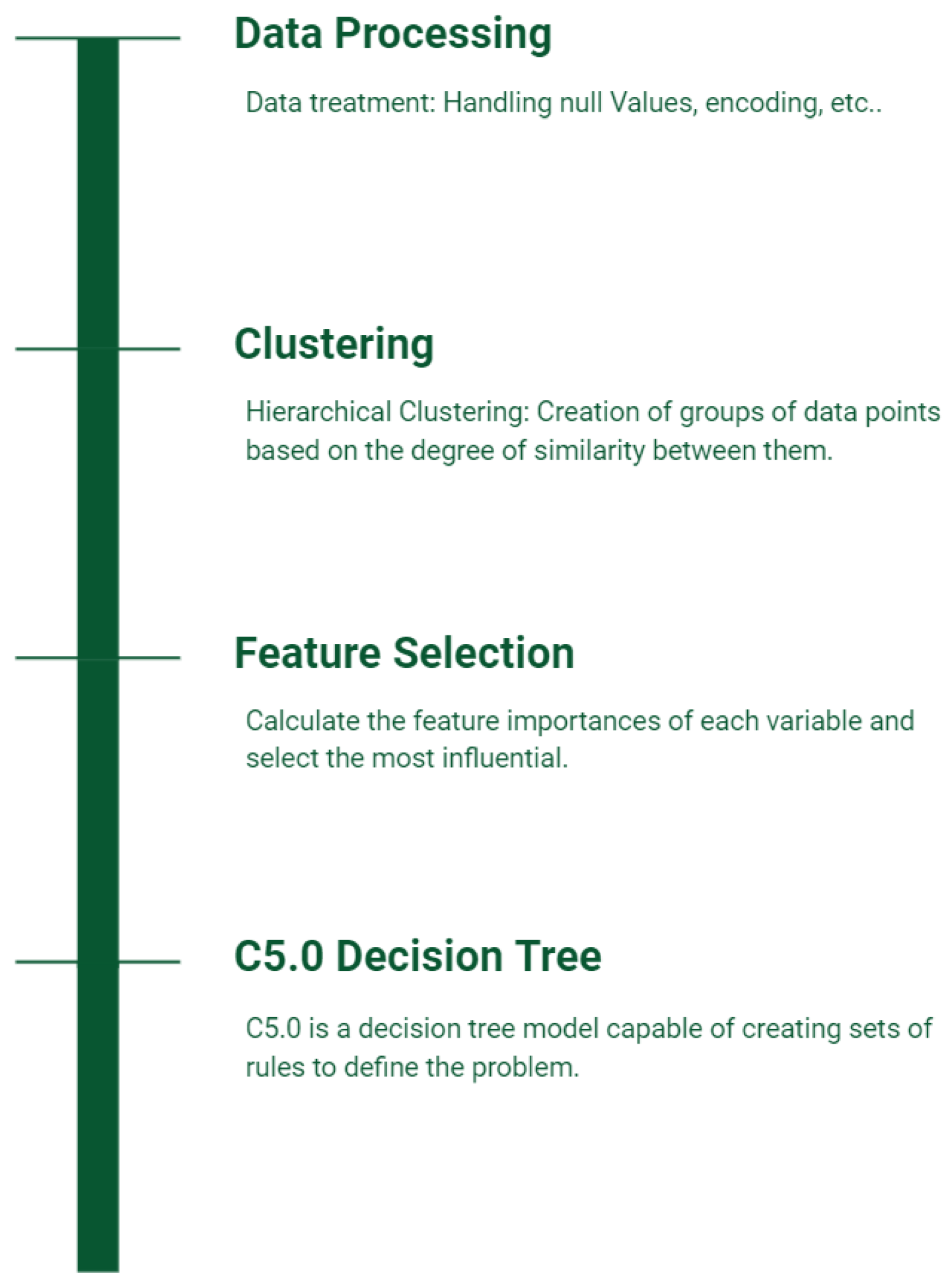
This section presents the proposed approach to find the most influential factors for accident severity and representing those factors in rule sets. Figure 1 illustrates the four stages of the proposed work, namely, data processing, clustering, feature selection, and rule generation.
Data processing is a common step in any study of this kind. For this stage, the data are cleaned and prepared so that it can be properly applied without problems to a machine learning model. This treatment consists of handling null values, encoding values, assigning types to variables, among other changes that are necessary for the correct reading of data by the algorithms.
Clustering or grouping of data is the creation of groups of data defined by their degree of similarity. The main objective of this step is to facilitate the creation of rules for each cluster by the machine learning algorithms.
Feature selection or variable selection consists in identifying the most important/ discriminatory variables in order to simplify the models and eliminate non-impact variables.
Finally, the last step applies the C5.0 algorithm to generate rules. These rules are formed by conditions of several variables to obtain a given class; thus, allowing new ideas and information about the data.
3.1. Dataset
The data used consists of 28,102 observations of traffic accidents from 2016 to 2019 containing various data sources such as, weather, road, driver, victim, and vehicle information, along with many other variables.
Various variables were chosen from this data and new variables were constructed based on this data.
In summary the following variables were used:
- “SeasonMov”—Weekends and holidays between May and September.
- “WorkHours”—Between 7 h and 20 h, excluding weekends and holidays.
- “School”—If accident occurred during school hours.
- “WindSpeed”—Wind speed in m/s on the nearest hour.
- “AirTemp”—Air temperature in ºC, nearest hour.
- “Parking”—Accident occurred in a parking lot.
- “TypeAcid”—Type of accident (collision, crash, or run over).
- “TotalDrivers”—Total number of drivers involved.
- “TypePlace”—Urban or rural.
- “RainQuant”—Precipitation amount in mm on previous hour.
- “HitAndRun”—A driver escaped the scene after the hit.
- “WeekDay”—Week day (1 to 7).
- “County”—County where accident occurred.
- “Month”—Month when accident occurred (1 to 12).
- “HourNear”—Nearest hour.
- “Motorcycle”—Accident involved motorcycle or similar.
- “LightVehicle”—Accident involved light vehicles.
- “HeavyVehicle”—Accident involved heavy vehicles.
- “RoadType”—Type of road.
- “Severity”—Accident severity.
The variable “Severity” is the dependent variable that will classify the accidents with or without victims.
3.2. Clustering
In this section, we explain some methods for clustering and respective algorithms.
Clustering is a common task of unsupervised learning, and unlike supervised learning, it does not require labeled dataset to work, instead, it discovers patterns on its own. Clustering is the process of grouping data points based on the similarity between them. The result of clustering will be groups of similar data points called clusters.
There are various types of Clustering algorithms, the most common being:
- Partitioning methods.
- Hierarchical clustering.
- Density-based clustering.
Partitioning clustering groups a user specified number of clusters k based on a criterion function. Hierarchical clustering builds a hierarchy of clusters and can be represented in dendrograms. Density-based clustering groups together data points that are in a dense region of a data space. Low density regions separate the clusters and are classified as noise. For a more detailed overview consider for instance [22].
For this specific approach, the Silhouette Index [23] was used as an evaluation measure to compare the performance of the agglomerative hierarchical clustering and the k-means algorithms. The silhouette index ranges from [−1, 1], with −1 indicating poor consistency within clusters and 1 indicating excellent consistency within clusters. Values near 0 suggest overlapping clusters.
When both algorithms were applied to the dataset and the silhouette index of the resulting groups was calculated, both approaches had a similar maximum value. Because none of the methods produced better indexes than the other in this circumstance, hierarchical clustering was selected.
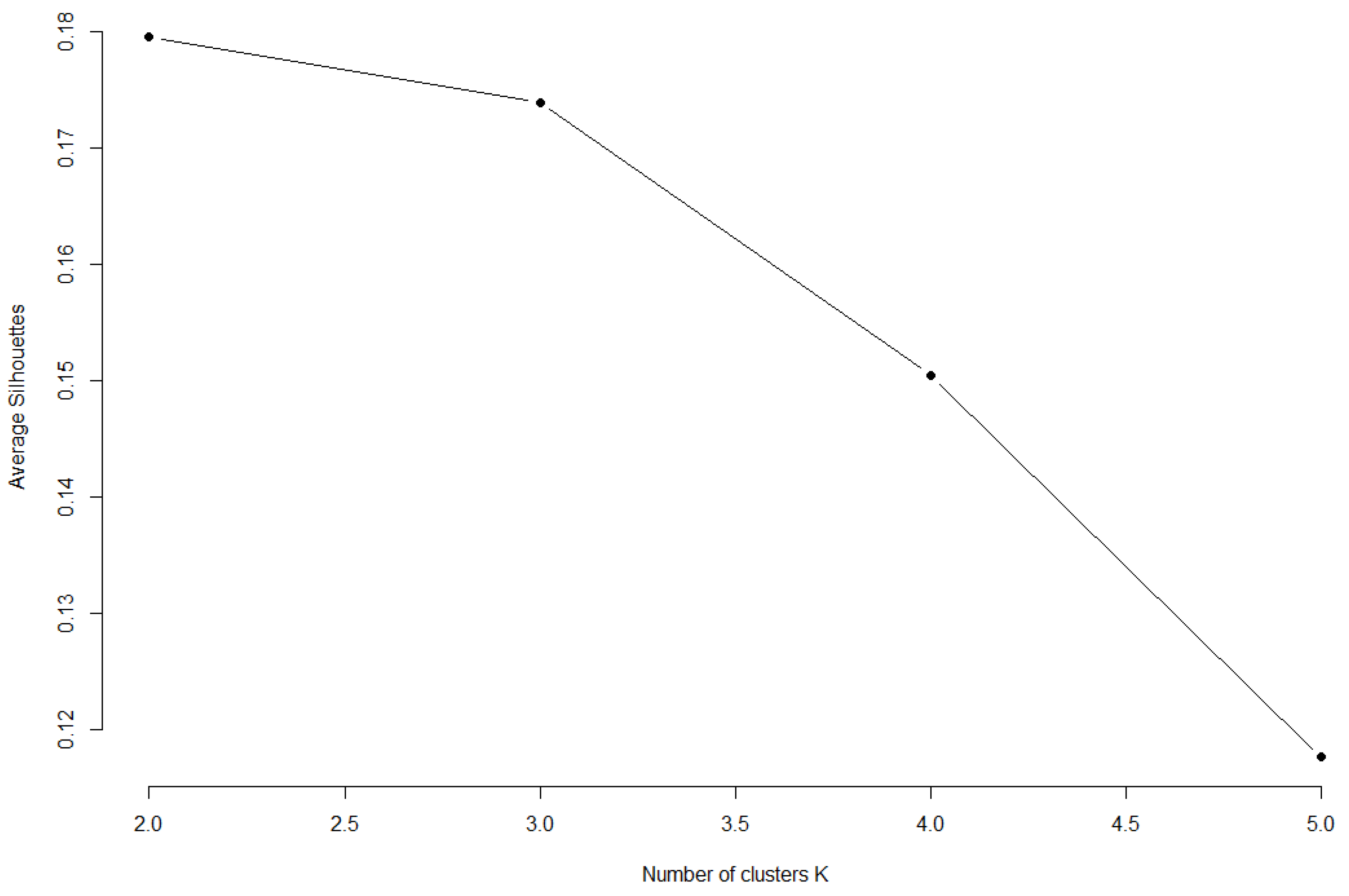
When deciding on the number of groups, it was discovered that the two-cluster models produced the best silhouette index results for both algorithms. The fluctuation of the silhouette index and the number of clusters for hierarchical clustering is shown in Figure 2.
The data were then separated into two clusters, each with 20,732 and 7371 observations, with a 0.18 silhouette index.
3.3. Feature Selection
The most influential variables of each cluster are selected in the next step. The “feature importance”, which reflects the relevance of each variable, was calculated using random forest.
Random forests or random decision forests [24] are an example of ensemble learning technique for classification, regression, and other tasks that operate by combining a collection of random decision trees at training time to achieve high classification accuracy. For classification tasks, the random forest’s output is the class chosen by the majority of trees.
In a regression or classification problem, random forests may also be used to rank the importance of predictors/variables [25]. Based on the mean decrease accuracy (MDA) values, we select the most influential variables in each cluster using the R package “randomForest”. The MDA values of a variable tell us how much that particular variable reduces/decreases the accuracy of the model if removed.
The resulting variables for the first cluster are:
- Motorcycle.
- TypeAcid.
- HitAndRun.
- WorkHours.
- HeavyVehicle.
- TypePlace.
The resulting variables for the second smaller cluster are:
- Motorcycle.
- TypeAcid.
- HitAndRun.
- AirTemp.
- LightVehicle.
- SeasonMov.
We also calculated the feature importance for the whole data set. This second experiment basically ignored the clustering from the previous stage. Its main features are:
- Motorcycle.
- TypeAcid.
- HitAndRun.
- AirTemp.
- HourNear.
- LightVehicle.
- TypePlace.
- RoadType.
3.4. Rule Generation Models
Machine learning algorithms usually fall into two categories, supervised and unsupervised learning. As previously mentioned, supervised learning uses labeled data, or more specifically, data points with correct outputs as opposed to unsupervised learning, which is not a requirement [26]. Supervised learning algorithms attempt to classify and predict the target output values based on the relationship between the outputs and inputs, which is learned from previous data sets.
Classification is a common supervised learning task that separates the data using a discrete target variable, more specifically, binary classification, which has two possible output values, for example, “yes or no”, “0 or 1”. As an illustration of such algorithms, consider for instance logistic regression, random forest, support vector machines, decision trees, naive Bayes, etc. [27]. In this particular work, the output values are “No Victims” or “With Victims”, i.e., 0 or 1, for the “Severity” variable.
The algorithm used in this approach was the C5.0 algorithm, which creates decision trees and can also generate rules.
3.5. Models Results
Models for each cluster and the entire data set were built; however, it is vital to note that the created rules in the models applied to each cluster should not be interpreted as a general rule because they only apply to a part of the data (cluster).
For cluster 1, four rules were created, and Table 2 depicts its result.
Following a thorough examination of some of these rules, the following findings were reached: When we apply the first rule to the complete dataset, we find that this holds true for 83 percent of the accidents. When the requirement “Motorcycle = 1” is removed from the rule, the result is substantially similar. In general, 63% of trampling have victims; therefore, this rule indicates that trampling that occur within the localities are more severe. This observation is backed up by Rule 3. The possibility of being run over by animals in rural areas that do not produce “victims” could explain this observation.
A total of of all accidents result in fatalities. When it comes to accidents involving motorcycles or similar vehicles, the number jumps to . As a result, when motorcycles are involved, accidents are more serious. This is shown by Rules 2 and 4.
For cluster 2, three rules were created, and Table 3 shows the result.
Cluster 2’s results are comparable to Cluster 1’s results in certain ways. Again, we see how serious accidents are when motorcycles or similar vehicles are involved (Rules 1 and 3). As previously said, 63 percent of pedestrians run over become victims, which is a far larger percentage than crashes and collisions, as this rule demonstrates.
Finally, Table 4 shows results of the model applied to the whole dataset.
The severity of pedestrian accidents is addressed under Rules 1 and 4. The severity of incidents involving motorbikes and similar vehicles is addressed under Rules 2, 3, and 6.
Rule 5 is particularly intriguing: there have been 3990 hit and run incidents, yet only 233 (about 6%) have resulted in victims. As previously stated, casualties are present in 21% of all accidents.
4. Prediction Model
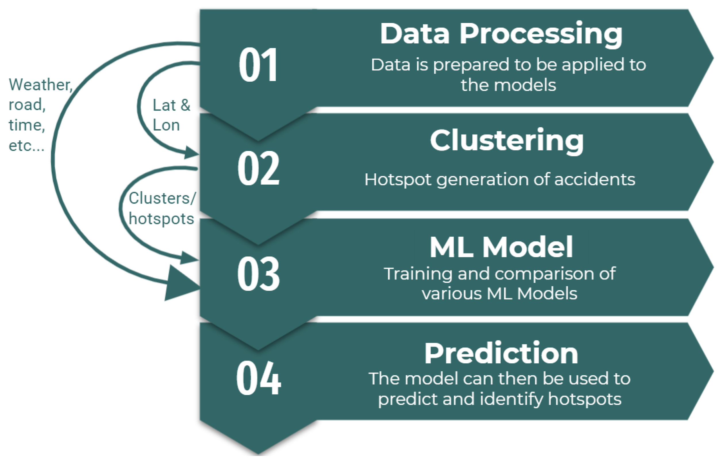
After the generation of rules and better understanding of the dataset, another approach was created that aims to create a system capable of predicting traffic accident hotspots. Figure 3 gives an outlook of the overall workings of the system.
The Figure shows the clustering algorithm taking as input the geographical coordinates of the accidents and adding its output as input of the predictive model. Moreover, the data inputs of the predictive model also contain weather, road, and time information. Finally, given a date and time, the system will then predict and map the traffic accidents hotspots.
This work can be divided into data processing, clustering, predictive model training, and prediction. In the following sections, we briefly explain these stages.
4.1. Data Processing
Again, the same data containing the 28,102 observations of traffic accidents were prepared for this new approach. The main criteria for variable selection in this is approach is including variables that can be predicted for a set location and future date/time such as weather; thus, in this case, information regarding the date, time, weather condition, and location of the accidents are the main features. In summary, the following new variables were used:
- “Latitude/Longitude”—The Latitude and Longitude coordinates.
- “WindDirection”—Average Wind Direction (Degrees).
- “DayOfYear”—Day of year (1 to 365/366).
- “Hour”—Nearest hour.
- “Day”—Day of month.
- “RegularSpeed”—Historical regular speed in segment in km/h.
- “DayShift”—Periods of the day.
- “Year”—Year when accident occurred.
- “HasDivider”—Road has a divider that separates the traffic flow in opposite direction.
- “TrafficPeak”—Accident occurred in a rush hour.
- “PathType”—Whether it occurred in a turn or straight.
- “Holidays”—The day is an holiday.
- “DamagedRoad”—Whether the road as significant damage.
Further, variables described previously were used: SeasonalMov, WorkHours, School, AirTemp, TypePlace, RainQuant, DayOfWeek, Month, Hour, and RoadType. See Section 3.1 for more details.
Another important task is the generation of the negative samples. Negative samples are necessary for the binary classification models, as the original dataset contains only positive samples (actual accidents). For the negative sampling generation, we followed an approach used in [28] that basically generates three negative samples for each accident randomly changing the date and time and consequently obtaining updated weather conditions for said date/time; making sure there are no negative samples equal to existing positive samples.
Various tests were conducted with a different number of negative samples including full negative sampling (for every single hour when no accidents occurred). Results showed that having three times negative samples than positive samples had the best balance of sensitivity, specificity, and accuracy metrics in the model evaluation stage.
4.2. Clustering
One of the first steps in road safety improvement is the identification of hotspots or hazardous road locations, also known as black spots. There is no commonly agreed definition of a ‘hotspot’ in the road accident literature [29]. Elvik, R. [30] conducted a survey on various European countries to describe the various hotspots definitions. The author included Portugal in the survey, where one of the definitions used was road segments with a maximum length of 200 m, with five or more accidents and a severity index greater than 20, in one year. Severity index weights fatal accidents with a a greater value than accidents with only slight injuries. The detection is performed with the sliding window technique that moves along the road. This and other definitions are usually applied depending on the road characteristics, typically highways, and the techniques are not optimal to deal with multiple road types or road junctions.
Another way to find accident hotspots is to detect areas with high accident density. As mentioned in Section 2, the paper by Szénási and Csiba [20] uses a clustering method (DBSCAN) in order to find accident hotspots using the accident’s GPS coordinates. This gives us the possibility to use the whole dataset regardless of road characteristics and group accidents that are in proximity to one another. This hotspot concept and this method of identifying hotspots are also used in our work.
DBSCAN works with two important parameters: epsilon and minimum points. Epsilon or eps, determines the maximum distance between two points to be considered neighbors (belonging to the same cluster). Minimum points or MinPts determine the minimum data points that are necessary to form a cluster. Otherwise, the data points are declared as noise (do not form a cluster).
There are no general methods for determining the ideal Eps and MinPts in this situation, as we want a certain area size for the clusters. Using such methods such as silhouette score, elbow curve, etc., would result in a few very large clusters of a few kilometers wide. The idea is to have a cluster size no larger than a few road segments or intersections, although it might still occur.
After a few experiments with changing Eps and MinPts, we found that assigning 150 m to Epsilon and 10 accidents as minimum points provided an acceptable size for the clusters, similar to the area size of a few intersections or road segments. Basically, a cluster will have at least 10 accidents, and in each cluster, the accidents will have in a 150 m radius, at least one other accident of the same cluster.
4.3. The Model
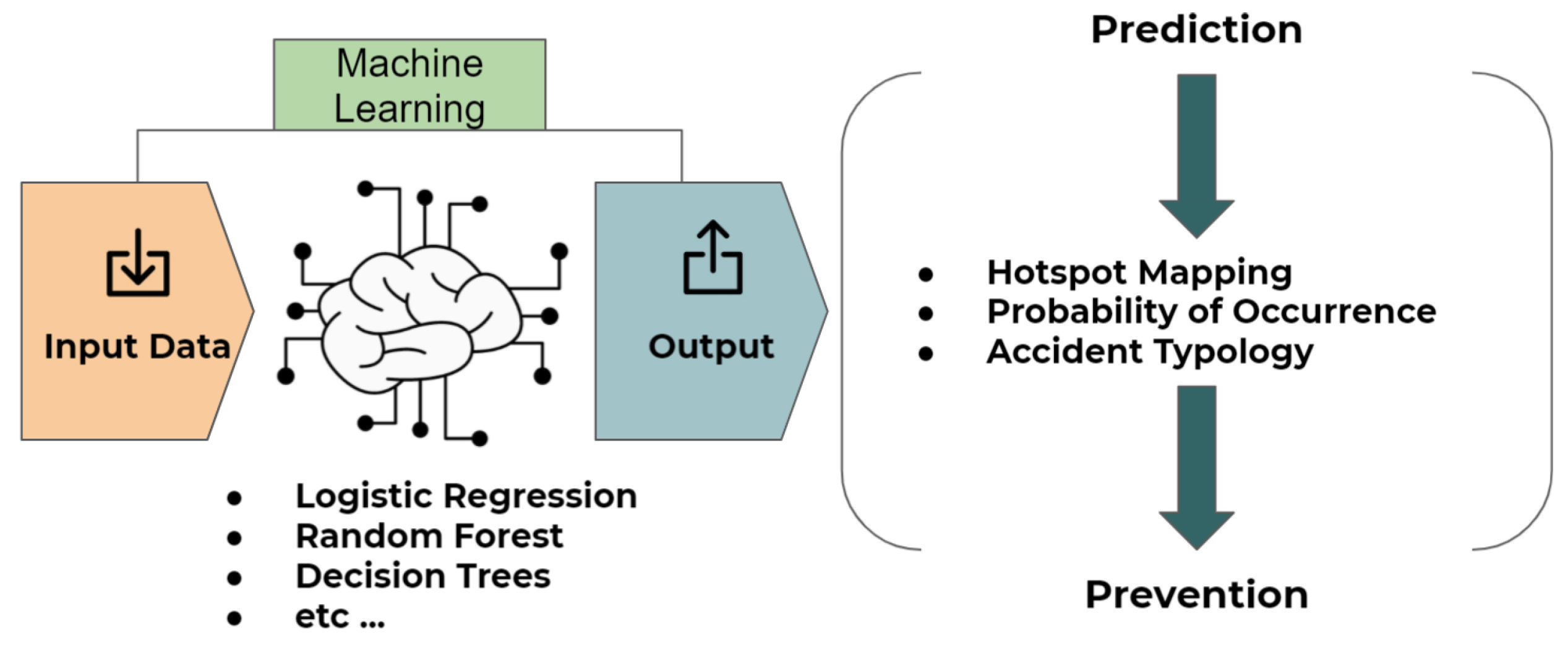
This work falls under the category of a classification problem, as we want to classify which hotspots are “activated” in given circumstances.
Figure 6 describes the general topic of the classification problem specific to this work.
As we want to comprehensively validate and compare our models, we consider various performance metrics such as accuracy, sensitivity, specificity, precision, false positive rate, and AUC Score. To calculate these metric’s values the following measures are needed:
- True positives (TP)—The model correctly predicts the positive class.
- False positives (FP)—The model of incorrectly predicts the positive class.
- True negatives (TN)—The model of correctly predicts the negative class.
- False negatives (FN)—The model of incorrectly predicts the negative class.
After counting the number of the different outcomes the following performance metrics can be calculated:
AUC score (area under the curve) measures the area underneath the ROC curve (receiver operating characteristic curve), which is a graph that plots the TPR and FPR. The higher the AUC value, the better the model is at distinguishing crashes and non-crashes.
4.4. Model Results
The initial tests were made using logistic regression, decision trees, and random forests, the latter having the better results. The data were split into 70% training data and 30% test data. The evaluation can be seen in Table 5.
Results in Table 5 show that random forests have the best results. Its sensitivity and specificity tells us that the model is quite conservative, having many false negatives, but is quite good at preventing “false alarms” with a false positive rate (FPR) of 3%.
An advantage of random forests is the visualization of the feature importance, as shown in Figure 7. Observing this figure, we can make changes to the dataset eliminating features that do not influence the results while having a better understanding of which features are the most influential.
5. Discussion
The results from the rule generation model were successful in finding patterns for fatal and non-fatal traffic accidents. According to the model, pedestrian accidents and accidents involving motorcycles are the main factors that have a higher chance of resulting in victims, whereas most collisions and crashes that do not involve motorcycles do not result in injuries. Intriguingly, hit-and-run incidents are less likely to result in a victim. These results were discussed and validated by the MOPREVIS project team, which include road safety experts from GNR.
By clustering the data prior to the generation of the rules will facilitate the rule generation by the model but it should be taken into account that such rules should not be interpreted as a general rule of the entire data and should be tested for its veracity afterwards.
Comparing this results to the similar work by Siam et al. [3], both theirs and our work reached different conclusions and highlighted factors, which is expected as there are differences in the data itself and how it was processed and divided. For example they found that national/regional/rural roads with no divider have more chances of fatal accidents. The same can be said about other factors highlighted by researchers in Section 2. Overall, these results can help us understand hidden aspects of our data, that are not easily obtained in statistical data distributions or common univariate/bivariate analysis.
In the accident prediction study, we have used a dataset containing vehicle accidents in the road network of the district of Setúbal, as well as historical weather information for such accidents. Using this dataset, we extracted the relevant features for accident prediction and created positive examples, corresponding to the occurrence of a collision, single vehicle crash or pedestrian accidents, and negative examples corresponding to non-occurrences of accidents. Then we focused on random forest algorithm as it proved to be a popular choice. The model proved to be quite conservative with a false positive rate (FPR) of 3%, specificity of 0.97, and sensitivity of 0.08, reaching an accuracy of 73%; further development of this approach is required to improve these results.
When comparing these results to literature, it is important to note that, as most examples belong to the negative class, the model that contains the higher negative/positive samples ratio is usually the one with the highest accuracy. Considering this, our work achieved an excellent FPR when compared to other works [2,9,14] mentioned in Section 2, Table 1, while sensitivity is still not in an acceptable range.
Future Work
Initial tests are quite inconsistent and more work and data are required in this task before obtaining conclusive results. For future work, more recent data (2020/2021) will be provided to us that will allow us to improve the proposed work. Since we have highlighted motorcycles accidents as the main factor influencing accident severity it would be interesting to include traffic parameters and intensity to our approaches and compare the results to the results of Theofilatos et al. (2016) [6], which has identified traffic flow and speed variations to influence powered two-wheeler (PTW) crashes. Additional machine learning algorithms and especially neural networks and deep learning approaches will also be applied as it has proven to be successful and sometimes outperforming simpler algorithms [14,15,16]. Further, other paths may be taken, such as using crash frequency as dependent variable, which is also a popular approach in literature.
Author Contributions
Conceptualization, D.S., J.S., P.Q. and V.B.N.; methodology, D.S., J.S., P.Q. and V.B.N.; investigation, D.S., J.S., P.Q. and V.B.N.; data curation, D.S., J.S., P.Q. and V.B.N.; writing—original draft preparation, D.S.; writing—review and editing, D.S., J.S., P.Q. and V.B.N.; supervision, J.S., P.Q. and V.B.N.; All authors have read and agreed to the published version of the manuscript.
Funding
This work is financed by National Funds through the Portuguese funding agency, FCTFundação para a Ciência e a Tecnologia, under the project with reference FCT DSAIPA/DS/0090/2018, “MOPREVIS—Modelação e Predição deAcidentes de Viação no Distrito de Setúbal”.
Institutional Review Board Statement
Not applicable.
Informed Consent Statement
Not applicable.
Data Availability Statement
Restrictions apply to the availability of these data. Data was obtained from the Portuguese GNR in the context of the MOPREVIS project.
Acknowledgments
The authors would like to thank project “MOPREVIS—Modelação e Predição de Acidentes de Viação no Distrito de Setúbal”, with reference FCT DSAIPA/DS/0090/2018, financed by the Foundation for Science and Technology (FCT) within the scope of the National Initiative on Digital Skills e.2030, Portugal INCoDe.2030.
Conflicts of Interest
The authors declare no conflict of interest.
Abbreviations
The following abbreviations are used in this manuscript:
| DT | Decision trees |
| RF | Random forests |
| BRF | Balanced random forest |
| XGB | eXtreme gradient boosting |
| CART | Classification and regression trees |
| LR | Logistic regression |
| NB | Naive Bayes |
| NNC | nearest neighbor classification |
| SVM | support vector machine |
| kNN | k-nearest neighbor |
| CNN | Convolutional neural networks |
| LSTM | long-short term memory |
| DBSCAN | Density-based spatial clustering of applications with noise |
| MOPREVIS | Modeling and Prediction of Road Accidents in the District of Setúbal |
| GNR | National Republican Guard |
| FCT | Foundation for Science and Technology |
| AI | Artificial intelligence |
| LSTM | Long short-term memory |
| ConvLSTM | Convolutional LSTM network |
| DOT | Department of Transportation |
| RWIS | Roadway Weather Information System |
| AADT | Annual average daily traffic |
| MDA | Mean decrease accuracy |
| FPR | False positive rate |
| HSID | Hotspot identification |
| TPR | True Positive Rate |
| PTW | Powered Two-Wheeler |
| MNL | Multinomial Logit |
| EB | Empirical Bayes |
References
- Moprevis. Available online: https://moprevis.uevora.pt/en/ (accessed on 2 August 2021).
- Hébert, A.; Guédon, T.; Glatard, T.; Jaumard, B. High-Resolution Road Vehicle Collision Prediction for the City of Montreal. In Proceedings of the 2019 IEEE International Conference on Big Data (Big Data), Los Angeles, CA, USA, 9–12 December 2019. [Google Scholar]
- Siam, Z.S.; Hasan, R.T.; Anik, S.S.; Dev, A.; Alita, S.I.; Rahaman, M.; Rahman, R.M. Study of Machine Learning Techniques on Accident Data. In Advances in Computational Collective Intelligence; Hernes, M., Wojtkiewicz, K., Szczerbicki, E., Eds.; Springer International Publishing: Cham, Switzerland, 2020; pp. 25–37. [Google Scholar]
- Xu, C.; Wang, W.; Liu, P. Identifying crash-prone traffic conditions under different weather on freeways. J. Saf. Res. 2013, 46, 135–144. [Google Scholar] [CrossRef] [PubMed]
- Yu, R.; Xiong, Y.; Abdel-Aty, M. A correlated random parameter approach to investigate the effects of weather conditions on crash risk for a mountainous freeway. Transp. Res. Part C Emerg. Technol. 2014, 50, 68–77. [Google Scholar] [CrossRef]
- Theofilatos, A.A.; Yannis, G. Investigation of Powered-Two-Wheeler accident involvement in urban arterials by considering real-time traffic and weather data. Traffic Inj. Prev. 2016, 18, 293–298. [Google Scholar] [CrossRef] [PubMed]
- Theofilatos, A.; Graham, D.; Yannis, G. Factors Affecting Accident Severity Inside and Outside Urban Areas in Greece. Traffic Inj. Prev. 2012, 13, 458–467. [Google Scholar] [CrossRef]
- Iranitalab, A.; Khattak, A. Comparison of four statistical and machine learning methods for crash severity prediction. Accid. Anal. Prev. 2017, 108, 27–36. [Google Scholar] [CrossRef] [PubMed]
- Lin, L.; Wang, Q.; Sadek, A. A Novel Variable Selection Method based on Frequent Pattern Tree for Real-time Traffic Accident Risk Prediction. Transp. Res. Part C Emerg. Technol. 2015, 55, 444–459. [Google Scholar] [CrossRef]
- Chang, L.Y.; Chen, W.C. Data mining of tree-based models to analyze freeway accident frequency. J. Saf. Res. 2005, 36, 365–375. [Google Scholar] [CrossRef] [PubMed]
- Caliendo, C.; Guida, M.; Parisi, A. A crash-prediction model for multilane roads. Accid. Anal. Prev. 2007, 39, 657–670. [Google Scholar] [CrossRef]
- Silva, P.; Andrade, M.; Ferreira, S. Machine learning applied to road safety modeling: A systematic literature review. J. Traffic Transp. Eng. (Engl. Ed.) 2020, 7, 775–790. [Google Scholar] [CrossRef]
- Theofilatos, A. Incorporating real-time traffic and weather data to explore road accident likelihood and severity in urban arterials. J. Saf. Res. 2017, 61, 9–21. [Google Scholar] [CrossRef]
- Theofilatos, A.A.; Chen, C.; Antoniou, C. Comparing Machine Learning and Deep Learning Methods for Real-Time Crash Prediction. Transp. Res. Rec. J. Transp. Res. Board 2019, 2673, 036119811984157. [Google Scholar] [CrossRef]
- Ren, H.; Song, Y.; Wang, J.; Hu, Y.; Lei, J. A Deep Learning Approach to the Citywide Traffic Accident Risk Prediction. In Proceedings of the 2018 21st International Conference on Intelligent Transportation Systems (ITSC), Maui, HI, USA, 4–7 November 2018; pp. 3346–3351. [Google Scholar] [CrossRef] [Green Version]
- Yuan, Z.; Zhou, X.; Yang, T. Hetero-ConvLSTM: A Deep Learning Approach to Traffic Accident Prediction on Heterogeneous Spatio-Temporal Data. In Proceedings of the KDD’18: 24th ACM SIGKDD International Conference on Knowledge Discovery & Data Mining, New York, NY, USA, 24 August 2018; Association for Computing Machinery: New York, NY, USA, 2018; pp. 984–992. [Google Scholar] [CrossRef]
- Gutierrez-Osorio, C.; Pedraza, C. Modern data sources and techniques for analysis and forecast of road accidents: A review. J. Traffic Transp. Eng. (Engl. Ed.) 2020, 7, 432–446. [Google Scholar] [CrossRef]
- Kumar, S.; Toshniwal, D. A data mining approach to characterize road accident locations. J. Mod. Transp. 2016, 24, 43–56. [Google Scholar] [CrossRef] [Green Version]
- Montella, A. A comparative analysis of hotspot identification methods. Accid. Anal. Prev. 2010, 42, 571–581. [Google Scholar] [CrossRef] [PubMed]
- Szenasi, S.; Csiba, P. Clustering Algorithm in Order to Find Accident Black Spots Identified By GPS Coordinates. In Proceedings of the 14th GeoConference on Informatics, Geoinformatics, and Remote Sensing, Ilza, Poland, 19–25 June 2014; Volume 1. [Google Scholar] [CrossRef]
- Roshandel, S.; Zheng, Z.; Washington, S. Impact of real-time traffic characteristics on freeway crash occurrence: Systematic review and meta-analysis. Accid. Anal. Prev. 2015, 79, 198–211. [Google Scholar] [CrossRef] [PubMed]
- Sisodia, D.; Singh, L.; Sisodia, S. Clustering Techniques: A Brief Survey of Different Clustering Algorithms. Int. J. Latest Trends Eng. Technol. 2012, 1, 82–87. [Google Scholar]
- Rousseeuw, P. Silhouettes: A Graphical Aid to the Interpretation and Validation of Cluster Analysis. J. Comput. Appl. Math. 1987, 20, 53–65. [Google Scholar] [CrossRef] [Green Version]
- Ho, T.K. Random decision forests. In Proceedings of the 3rd International Conference on Document Analysis and Recognition, Montreal, QC, Canada, 14–16 August 1995; Volume 1, pp. 278–282. [Google Scholar] [CrossRef]
- Breiman, L. Random Forests. Mach. Learn. 2001, 45, 5–32. [Google Scholar] [CrossRef] [Green Version]
- Kotsiantis, S.; Zaharakis, I.; Pintelas, P. Machine learning: A review of classification and combining techniques. Artif. Intell. Rev. 2006, 26, 159–190. [Google Scholar] [CrossRef]
- Sarker, I. Machine Learning: Algorithms, Real-World Applications and Research Directions. SN Comput. Sci. 2021, 2, 1–21. [Google Scholar] [CrossRef]
- Yuan, Z.; Zhou, X.; Yang, T.; Tamerius, J. Predicting Traffic Accidents Through Heterogeneous Urban Data: A Case Study. In Proceedings of the 6th international workshop on urban computing (UrbComp 2017), Halifax, NS, Canada, 13–17 August 2017. [Google Scholar]
- Anderson, T. Kernel density estimation and K-means clustering to profile road accident hotspots. Accid. Anal. Prev. 2009, 41, 359–364. [Google Scholar] [CrossRef] [PubMed]
- Elvik, R. A Survey of Operational Definitions of Hazardous Road Locations in Some European Countries; Accident Analysis & Prevention: Amsterdam, The Netherlands, 2008. [Google Scholar]
Figure 1.
Description of the rule generation approach.

Figure 2.
Silhouette index variation and number of clusters.

Figure 3.
Description of the hotspot prediction approach.

Figure 4.
Overview of the clusters in the whole district.

Figure 5.
Zoom of the map that shows an acceptable size for the clusters (three separate clusters).

Figure 6.
Overview of the classification problem is this work.

Figure 7.
Random forest feature importance.


Table 1.
Description of systematized papers (accident occurrence).
| Reference | Algorithms Used | Imbalance Ratio | Performance (Best Model) |
|---|---|---|---|
| Hébert et al. (2019) | BRF, RF, XGB | 42:1 | 85% Acc., 15% FPR |
| Lin and Wang (2017) | RF, kNN, Bayes net | 3.3:1 | 61% Acc., 38% FPR |
| Theofilatos et al. (2019) | kNN, NB, DT, RF, SVM, LR, NN, DNN | 2:1 | 68.95% Acc., 52% TPR, 77% TNR |
Table 2.
Rule results for Cluster 1.
| Rule n° | Rule | Obs. n° | Error % | Class |
|---|---|---|---|---|
| 1 | Trampling in urban areas, no motorcycles involved | 460 | 15% | With Victims |
| 2 | Motorcycles involved | 1575 | 37% | With Victims |
| 3 | Trampling in rural areas | 263 | 16% | No Victims |
| 4 | Collisions and crashes, no motorcycles involved | 18,434 | 16% | No Victims |
Table 3.
Rule results for Cluster 2.
| Rule n° | Rule | Obs. n° | Error % | Class |
|---|---|---|---|---|
| 1 | Motorcycles involved | 1133 | 24% | With Victims |
| 2 | Trampling | 247 | 26% | With Victims |
| 3 | Collisions and crashes, no motorcycles involved | 6030 | 9% | No Victims |
Table 4.
Rule results for the whole dataset.
| Rule n° | Rule | Obs. n° | Error % | Class |
|---|---|---|---|---|
| 1 | Trampling in urban areas | 681 | 17% | With Victims |
| 2 | Accidents With Motorcycles, no Light Vehicles involved | 915 | 19% | With Victims |
| 3 | Accidents With Motorcycles, no Hit and Run | 2525 | 30% | With Victims |
| 4 | Trampling | 977 | 37% | With Victims |
| 5 | Accidents with Light vehicles, with a Hit And Run | 3803 | 4% | No victims |
| 6 | Accidents without motorcycles | 25,395 | 16% | No Victims |
Table 5.
Model evaluation metrics.
| Model | Accuracy | AUC Score | Precision | Recall/ Sensitivity | Recall/ Specificity |
|---|---|---|---|---|---|
| Random Forest | 0.73 | 0.68 | 0.44 | 0.08 | 0.97 |
| Logistic Regression | 0.73 | 0.66 | 0.27 | 0.00 | 1.00 |
| Decision Trees | 0.65 | 0.55 | 0.35 | 0.34 | 0.76 |
Publisher’s Note: MDPI stays neutral with regard to jurisdictional claims in published maps and institutional affiliations. |
© 2021 by the authors. Licensee MDPI, Basel, Switzerland. This article is an open access article distributed under the terms and conditions of the Creative Commons Attribution (CC BY) license (https://creativecommons.org/licenses/by/4.0/).
Share and Cite
MDPI and ACS Style
Santos, D.; Saias, J.; Quaresma, P.; Nogueira, V.B. Machine Learning Approaches to Traffic Accident Analysis and Hotspot Prediction. Computers 2021, 10, 157. https://0-doi-org.brum.beds.ac.uk/10.3390/computers10120157
AMA Style
Santos D, Saias J, Quaresma P, Nogueira VB. Machine Learning Approaches to Traffic Accident Analysis and Hotspot Prediction. Computers. 2021; 10(12):157. https://0-doi-org.brum.beds.ac.uk/10.3390/computers10120157
Chicago/Turabian StyleSantos, Daniel, José Saias, Paulo Quaresma, and Vítor Beires Nogueira. 2021. "Machine Learning Approaches to Traffic Accident Analysis and Hotspot Prediction" Computers 10, no. 12: 157. https://0-doi-org.brum.beds.ac.uk/10.3390/computers10120157
Note that from the first issue of 2016, this journal uses article numbers instead of page numbers. See further details here.