
A Geometric Approach to Noisy EDM Resolution in FTM Measurements †


1
Cisco Systems, Research Triangle Park, NC 27560, USA
2
IMT Atlantique, IRISA, 35510 Cesson-Sévigné, France
3
Cisco Systems, 821 09 Bratislava, Slovakia
*
Author to whom correspondence should be addressed.
†
This paper is an extended version of our paper published in 16th Wireless and Mobile Computing, Networking And Communications (WiMob 2020).
Computers 2021, 10(3), 33; https://0-doi-org.brum.beds.ac.uk/10.3390/computers10030033
Submission received: 31 January 2021
/
Revised: 9 March 2021
/
Accepted: 9 March 2021
/
Published: 12 March 2021
(This article belongs to the Special Issue Selected Papers from 16th&17th Wireless and Mobile Computing, Networking And Communications (WiMob 2020&2021))
Abstract
:Metric Multidimensional Scaling is commonly used to solve multi-sensor location problems in 2D or 3D spaces. In this paper, we show that such technique provides poor results in the case of indoor location problems based on 802.11 Fine Timing Measurements, because the number of anchors is small and the ranging error asymmetrically distributed. We then propose a two-step iterative approach based on geometric resolution of angle inaccuracies. The first step reduces the effect of poor ranging exchanges. The second step reconstructs the anchor positions, starting from the distances of highest likely-accuracy. We show that this geometric approach provides better location accuracy results than other Euclidean Distance Metric techniques based on Least Square Error logic. We also show that the proposed technique, with the input of one or more known location, can allow a set of fixed sensors to auto-determine their position on a floor plan.
1. Introduction
With Global Positioning System (GPS) augmented with fusion techniques (cellular trilateration, dead reckoning, etc.), outdoor location has become a reality on a large part of the planet. Location is more challenged indoor. The ability for a personal device (phone, tablet) to display the user location is useful, but GPS availability is often limited indoor.
1.1. FTM Approach to Indoor Location
Alternative techniques have been sought for decades. Among them, 802.11-2016 [1] Fine Timing Measurement (FTM), expanded in the 802.11az amendment, defines a procedure for indoor location tracking based on Wi-Fi ranging. Wi-Fi is massively deployed all over the planet. With common spectrum available worldwide, more than 16 billion devices in use and more than 4 billion new supporting devices shipped each year, according to the Wi-Fi Alliance, it is expected than any personal device (phone or tablet) would support Wi-Fi, and that Wi-Fi would be available in about any public place, anywhere. As such, a location method relying on Wi-Fi technologies has all the chances of seeing a large adoption, and is therefore of high interest. With FTM, an initiating station (ISTA) exchanges frames with a responding station (RSTA) and uses the times of the exchanges to deduce its own position relative to the RSTA. Specifically, after negotiating the exchange parameters, ranging measurements operate through bursts. At the beginning of each burst, the RSTA sends a frame (at time ) that reaches the ISTA at time . The ISTA sends an acknowledgement frame at time , that reaches the RSTA at time . In the subsequent frame, the RSTA communicates the and values. The ISTA can now compute the time of flight of the exchange and its distance d to the RSTA by a simple:
where c refers to the speed of light. This computation is only valid if a number of conditions are met:
- The drift in timestamp measurement at the RSTA is linear. The RSTA provides a time value for its frames, but a clock time difference between the ISTA and the RSTA is inconsequential as only () is considered (thus the interval between the associated frames, not the local time at which each value was measured), removing the need for synchronized clocks. However, a difference in drift rate between the RSTA and ISTA clocks may cause the () and () intervals to be counted at different tic speeds [2], leading to time and therefore range imprecision.
- Each side can measure accurately the time of arrival (ToA) and the time of departure (ToD) of each frame. This time is measured as the arrival (or departure) at the antenna of the beginning of the first training symbol (the beginning of the frame preamble). As the part of the system that measures time is not located in the physical antenna, each system needs to be calibrated to account for the delay between the antenna and the time measurement module. This calibration is usually done in Line of Sight (LoS) conditions. Different factors (temperature, noise, etc.) may render this calibration only partially accurate, thus resulting in larger estimated distances than the ground truth [3].
- Measurements are done in LoS conditions. The distance between the ISTA and the RSTA should be a straight line. If the considered signal is instead a reflection, then distance accuracy is lost. 802.11az includes mechanisms to detect Line of Sight vs non-Line-of-Sight (nLoS) signals. 802.11-2016 FTM does not include such mechanism, causing in some cases the receiver to associate the ToA with the first strong reflected component instead of the weaker primary LoS component. In some other scenarios, the signal traverses a strong obstacle where c is different than in the air. With a technique where each nanosecond represents a travelled distance of approximately a foot (30 cm), such mismatch can contribute to ranging inaccuracies in a measurable way.
All these elements play a role in ranging accuracy and need to be accounted for, as will be shown in this work.
Once computation of the range to multiple RSTAs has been completed, the ISTA only knows its distance to a set of anchors, but does not know its location. FTM allows the RSTA to send its Location Configuration Information (LCI) to the ISTA, a geo-position and height element which content follows a format defined in RFC 6225 [4].
1.2. The Challenges of FTM for Indoor Location and this Article Contribution
The FTM procedure introduces the very problem that it aims to solve. Outdoor, Global Positioning System (GPS) technologies provide location information to mobile devices in most environments where LoS to GPS satellites can be established. Indoor, GPS becomes difficult to use for the same reason and devices cannot reliably establish their geo-position anymore. But FTM supposes that RSTAs, positioned indoor, can be configured with their correct geo-position. A common assumption is that these RSTAs would be Wi-Fi access points (APs). In fact, any other type of 802.11 device could support the RSTA function (digital signage, printers, Wi-Fi cameras, etc.). We will call all these objects sensors for simplicity. In most cases, these sensors would be positioned at a static location (or a location that changes only occasionally). Yet configuring their geo-position is difficult. These objects typically do not include a GPS sensor. Even if they would, GPS is challenged indoor. Many implementers are left with manual and time consuming techniques, where the geo-positions of points at the edge of the building are fist established (using mobile devices GPS functions outside, or high-resolution reference aerial pictures), then high precision ranging techniques (laser, Ultra Wide Band, etc.) are used to finally come to an evaluation of each sensor position and location. The process has to be reiterated each time an RSTA is moved or added.
Yet, as soon as the geo-position of one or more device is known, this paper shows that the other sensors can use FTM to self-locate one another, considerably simplifying the deployment of an FTM-ready infrastructure. Solving this problem implies seeding the system with one or more initial positions, which is trivial and can be achieved with a mobile device ranging to one or more RSTAs from outside the building. The solution also implies solving the issue of self-positioning, where the various anchors can reliably establish their respective position based on noisy environments. Thus, the contributions of this article are as follows: noting that pairwise FTM distance noise is not symmetrical, this paper first proposes to reduce the noise by identifying its contribution to geometric distortion of the triangles formed by AP sets, in a phase called Wall Remover. By identifying the effect of inner walls of FTM exchanges between AP pairs, this phase allows for the reduction of the effect of walls on FTM measurements. In a second phase, a recursive examination of all possible Euclidean distance matrices is conducted, to identify the anchors least affected by noise. By combining standard EDM techniques with geometric projections, this phase allows the selection of the best sub-matrices (least effected by remaining measurement noises) to compute the positions of anchors which are most likely to be accurate. From their position, the location of all other anchors is computed, leading to a better position accuracy than EDM resolution techniques alone.
An early version of this work was presented in [5]. In this article, we deepen our proof and extend the applicability of the method to different types of buildings. The rest of this article is organized as follows: Section 2 briefly examines possible techniques to augment GPS for indoor location. Section 4 details the general problem space of noisy Euclidian matrix completion. Section 5 explains our approach, with an asymmetry reduction phase and an algebro-geometric approach. Section 6 presents numerical validation through experimental measurements, and compares the accuracy of our proposed method to other classical Euclidean Distance Matrix (EDM) resolution methods. Section 7 concludes this paper.
2. Related Work
Outdoor location based on GPS can commonly provide accuracy down to a meter or less [3]. When nearing a building, the accuracy gets diluted as the building hides some GPS satellites from view [6]. Different augmentation techniques were proposed to limit this issue. For example, Liu et al. [7] proposed using detection of the building and comparison with publicly available aerial imagery to revert to meter precision. Other authors propose to use the known degradation pattern of the signal [8,9] to adjust the location calculation. Our measurements in this paper show that accuracy can be maintained at a sub-meter level in many cases, even near buildings. This will prove useful, as the method proposed in this paper uses outdoor GPS measurements as a final seed to reorient the graph formed by APs having computed their relative positions (but not knowing the position of the graph in the building). Indoor however, GPS accuracy depends heavily on the building structure (windows, floor size and plan etc.). In some scenarios, location can be obtained [7], but in most, the signal is lost. Other technologies are then commonly used to deploy anchors with known positions and perform measurements (signal or distance) against them [10,11]. FTM, studied in this paper, is one of such technologies.
Although FTM is intended for indoor location, the technology allows a mobile device, still outside and detecting GPS satellites, to range and seed its location to one or more indoor RSTAs. The idea of seeding GPS measurements from outdoor to indoor systems is not new, and has for example been studied in [12] and [13]. Once they have ranged to an initial known outdoor location, these RSTAs could range to one another and determine their relative position. Such task falls into the general domain of sensor location in a noisy environment. This field has been explored widely in multiple contexts, as it represents the need for several systems to evaluate their distance to one another, thus building a distance matrix, and then resolving the inconsistencies between measurements. In wireless technologies, the distance can be evaluated with a variety of techniques (time of flight measurements, signal estimations), but most of them are noisy, resulting in an imperfect, or incomplete, distance matrix. Resolving such matrix is a complex problem, which challenges are summarized in [14]. Ref [15] provides an overview of the main resolution techniques. In the particular case of sensor location, [16] shows that the problem can be convex if the dimension space is known, which is often the case for RSTAs in FTM (but not when using FTM alone, as we will show). An approach close to ours, to reduce the problem with sub-matrix spaces, is detailed in [7], although the proposed method is strictly algebraic (while we propose a geometric component). As the distances are organized in a matrix, algebraic approaches are natural. Some authors, like Doherty and al. [17], explore geometric resolutions in scenarios where link directionality matters. We will show that the addition of learning machine can considerably enhance the resulting accuracy.
3. Multidimensional Scaling (MDS) Background
This work focuses on FTM exchanges between fixed points. In this context, Wi-Fi access points and other static devices (e.g., digital signage) can be configured to play the role of ISTAs and RSTAs, alternating between one and the other and ranging to one another over time. As the points are fixed, and as each ranging burst takes a few hundreds of milliseconds (e.g., a burst of 30 exchanges would consume about 250 ms in good RF conditions), a large number of samples can be taken (e.g., a burst per minute represents 43,200 samples per 24-hour period). This flexibility allows for obtaining ranges between pairs far apart, and for which only a few exchanges succeed. From all exchanges, only the best (typically smallest) distance is retained, as will be seen later. The output of these FTM measurements is a network of nodes, among which nodes have a known position.
The measured distance between these nodes can be organized in a matrix that we will note . Conceptually, the set is similar to any other noisy Euclidean Distance Matrix (EDM). The set contains an exhaustive table of distances between points taken by pairs from a list of points x in N dimensions and for any point . Each point is labelled ordinally, hence each row or column of an EDM, i.e., , individually addresses all the points in the list. The main task of the experimenter is then to find the dimension N and construct a matrix of distances that on one hand best resolves the noise (which causes inconsistencies between the various measured pairs), and on the the other hand is closest to the real physical distances between points, called ground truth, and which matrix is noted D. Such task is one main object of Multidimensional Scaling (MDS).
MDS draws its origin from psychometrics and psychophysics. MDS considers a set of n elements and attempts to evaluate similarities or dissimilarities between them. These properties are measured by organizing the set elements in a multi-dimensional geometric object where the properties under evaluation are represented by distances between the various elements. MDS thus surfaces geometrical proximity between elements displaying similar properties in some dimension of an space. The properties can be qualitative (non-metric MDS, nMDS), where proximity may be a similarity ranking value, or quantitative (metric MDS, mMDS), where distances are expressed. This paper will focus on mMDS.
Two main principles lie at the heart of mMDS: the idea that distances can be converted to coordinates, and the idea that during such process dimensions can be evaluated. The coordinate matrix X is an object, where each row i expresses the coordinate of the point i in N dimensions. Applying the squared Euclidean distance equation to all points i and j in X (Euclidean distance , which we write for simplicity) allows for an interesting observation:
Applying this equation to the distance matrix D, noting the squared distance matrix for all , c an column vector of all ones, the column a of matrix X, noting e a vector that has elements , and writing the transpose of any matrix A, the equation becomes:
This observation is interesting, in particular because it can be verified that the diagonal elements of are , i.e., the elements of e. Thus, from X, it is quite simple to compute the distance matrix D. However, mMDS usually starts from the distance matrix D, and attempts to find the position matrix X, or its closest expression U. This is also FTM approach, that starts from distances and attempt to deduce location. As such, mMDS is directly applicable to FTM.
Such reverse process is possible, because one can observe that D, being the sum of scalar products of consistent dimensions, is square and symmetric (and with only positive values). This observation is intuitively obvious, as D expresses the distance between all point pairs, and thus each point represents one row and one column in D. These properties are very useful, because a matrix with such structure can be transformed in multiple ways, in particular through the process of eigendecomposition, by which the square, positive and symmetric matrix B of size can be decomposed as follows: , where matrix Q is orthonormal (i.e., Q is invertible and we have ) and is a diagonal matrix such that . Values of are the eigenvalues of B. Eigenvalues are useful to find eigenvectors, which are sets of individual non-null vectors that satisfy the property: , i.e., the direction of does not change when transformed by B.
In the context of MDS, this decomposition is in fact an extension of general properties of Hermitian matrices, for which real and symmetric matrices are a special case. A square matrix B is Hermitian if it is equal to its complex conjugate transpose , i.e., .
In terms of the matrix elements, such equality means that . A symmetric MDS matrix in obviously respects this property, and has the associated property that the matrix can be expressed as the product of two matrices, formed from one matrix U and its transpose , thus . Because this expression can be found, B is said to be positive semi-definite (definite because it can be classified as positive or negative, positive because the determinant of every principal submatrix is positive, and positive semi-definite if 0 is also a possible solution). A positive semi-definite matrix has non-negative eigenvalues.
This last property is important for mMDS and for the FTM case addressed in this paper. As can be rewritten as , it follows that non-null eigenvectors are orthogonal. As such, the number of non-null eigenvalues is equal to the rank of the matrix, i.e., its dimension. This dimension is understood as the dimension of the object studied by MDS. With FTM, this outcome determines if the graph formed by APs ranging once another is in 2 dimensions (e.g., all APs on the same floor, at ceiling level) or in 3 dimension (e.g., APs on different floors). In a real world experiment, B is derived from and is therefore noisy. But one interpretation of the eigendecomposition of B is that it approximates B by a matrix of lower rank k, where k is the number of non-null eigenvalues, which can then represent the real dimensions of the space where B was produced. This is because, if is the i-th column vector of Q (and therefore the i-th row vector of ), then can be written as:
And thus
Therefore, if eigenvalues are 0, so is their individual product, and an image of B can be written as:
C and B have the same non-null eigenvectors, i.e., C is a submatrix of B restricted to the dimension of B’s non-null eigenvalues. In noisy matrices, where distances are approximated, it is common that all eigenvalues will be non-null. However, the decomposition should expose large eigenvalues (i.e., values that have a large effect on found eigenvectors) and comparatively small eigenvalues (i.e., values that tend to reduce eigenvectors close to the null vector). Small eigenvalues are therefore ignored and considered to be null values that appear as non-zero because of the matrix noise.
An additional property listed above is that positive semi-definite matrices only have non-negative eigenvalues. In the context of MDS, this is all the more logical, as each eigenvector expresses one dimension of the space. However, noisy matrices may practically also surface some negative eigenvalues. The common practice is to ignore them for rank estimation, and consider them as undesirable but unavoidable result of noise. We will apply the same principles for measurements obtained with FTM. However, it is clear that the presence of many and/or large negative eigenvalues is either a sign that the geometric object studied under the MDS process is not Euclidian, or that noise is large, thus limiting the possibilities of using the matrix directly, without further manipulation.
Therefore, if from Equation (3) above, one defines , then an eigendecomposition of B can be performed as . As scalar product matrices are symmetric and have non-negative eigenvalues, one can define as a diagonal matrix with diagonal elements . From this, one can write The coordinates in U differ from those in X, which means that they are expressed relative to different coordinate systems. However, they represent the geometric object studied by MDS with the same dimensions and scale. Thus, a rotation can be found to transform one into the other.
With these transformations, mMDS can convert a distance matrix into a coordinate matrix, while estimating the space dimension in the process. Thus, classical mMDS starts by computing, from all measured distances, the squared distance matrix . The measured distance matrix is also commonly called, in MDS in general, the proximity matrix, or the similarity matrix. Next, a matrix called the J is computed, that is in the form where c is an column vector of all ones. Such matrix is a set of weights which column or row-wise sum is twice the mean of the number of entries n. This matrix has useful properties described in [18]. In particular, applied to , it allows the determination of the centered matrix , which is a transformation of around the mean positions of . This can be seen as follows:
By transposing J into the expression, it can easily be seen that, as and :
At this point, the distance matrix is centered. This phase has a particular importance for the method proposed in this paper, because we will see below that its direct effect is to dilute the noise of one pair into the measurements reported by other pairs, thus causing mMDS to fail in highly asymmetric measurements like FTM. mMDS then computes the eigendecomposition of . Next, the experimenter has the possibility to decide of the dimensions of the projection space ( or in our case, but the dimension can be any in mMDS). This can be done by arbitrarily choosing the m largest eigenvalues and their corresponding eigenvectors of B. This choice is useful when the experimenter decides to project the distance matrix into m dimensions, and has decided of what value m should be. Alternatively, the experimenter can observe all eigenvalues in B and decide that the dimension space matches all m large positive eigenvalues in B, ignoring the (comparatively) small positive eigenvalues, along with the null and negative eigenvalues as detailed in the previous section.
Then, if we write the matrix of these m largest positive eigenvalues, and the first m columns in Q (thus the matrix of eigenvalues matching the dimensions decided by the experimenter), the coordinate matrix is determined to be .
4. Problem Space Framework
4.1. mMDS Limitations in FTM Measurements
We note that mMDS is a family of techniques, with multiple possible variations, but all of them abide by the general core principles expressed in the previous section. These principles present properties of great value for multiple distance applications, but also three unsolvable limitations for indoor measurements like FTM: pairwise asymmetry is ignored, dimension space cannot be determined, and as the errors are centered, location accuracy is always typically poor. This section examines these issues in turn.
4.1.1. Pairwise Asymmetry
Although FTM does build a square distance matrix , the FTM distance matrix displays several specific properties. One such property is asymmetry. In most cases, measurements are unidirectional, one side acting as the initiator, the other as the responder. In the case of static anchors, the roles can be inverted at the conclusion of each exchange. The process repeats for each sensor pair. These exchanges are affected by localities. As the measurements are collected in a noisy environment, they suffer from the side effects of multipath. Although most sensors attempt to determine the first signal to establish the line of sight (and therefore shortest distance), it is common that strong multipath may drown that signal to a point where the receiver identifies the first strong reflection as the first signal. In an environment where the position of reflective surfaces cannot be predicted, such effect may affect differently each receiver. As a consequence, the initial distance matrix set is asymmetric, where, for many pairs, .
If obstacles or reflection sources are static (e.g., walls), such asymmetry cannot be resolved by continuous measurements or by averaging over a long period (asymmetry persists). In an implementation where FTM sensors are calibrated (i.e., where the computed distance in line of sight is close to, but never less than, the ground truth), a simple corrective measure consists to only consider the smaller value for each reported pair distance, thus allowing .
4.1.2. Dimension Determination
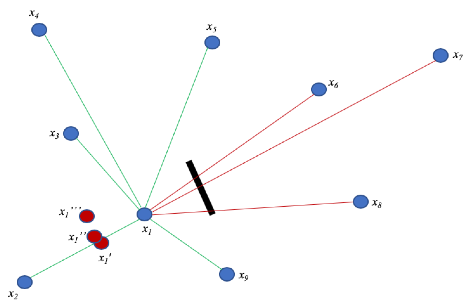
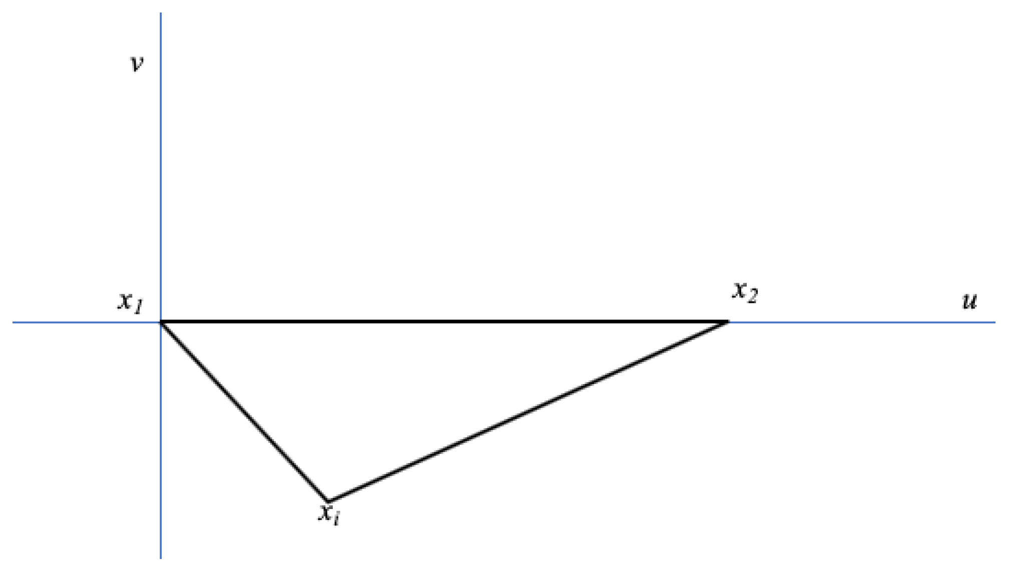
This approximation solves single pair distance inequalities, but indoor measurements surface another type of asymmetry. As illustrated in Figure 1, indoor walls are local objects. As the signal passes through a wall, it can be slowed down enough to induce an increased travel time between the ISTA and the RSTA, and thus a measured distance dilated by a factor (compared to the ground truth ) different than the dilation for another pair, between which a wall would not be found, and thus, for 3 APs i, j and l:
Algebraically, a similar dilation factor k for all measured distances would be ideal and would make the dilation easy to resolve. Each measured distance would then be a simple (dilated) single scalar representation of the ground value matrix. As:
Then would be a simple homothetic transformation of D, and our only task would be to find the scalar k, the dilation factor. But in real measurements, noise is not linear and each is affected by a different dilation. Finding individual values becomes challenging, even if we reduce the scope by half by making the hypothesis that as above (thus considering that the smallest distance is likely closest to the true LoS distance), and thus that . This geometry of the indoor space results in two additional major difficulties when attempting to use mMDS.
The first difficulty relates to dimension definition. FTM measurements are collected either in 2 dimensions (all APs or sensors at the same level, e.g., at ground or ceiling level on the same floor) or 3 dimensions (multi-floor scenario). One task is therefore to determine the dimensions of the collection space, expecting 2 or 3 as a result. However, the interference locality expressed before results in different inaccuracies between measurements. This problem is difficult to resolve. A common MDS approach in this case is to let the experimenter decide of the dimensions, then use the least square error technique to project the matrix in the assigned space. But this approach is only valid if the experimenter knows a priori the dimension n. In an indoor setting where RF travels in all directions and where distances are only measured by time of flight, such an arbitrary decision puts an unacceptable burden of knowledge on the FTM experimenter. Without knowing a priori , the determination of the vertical component of a set of sensors is only possible if happens to be small relative to .
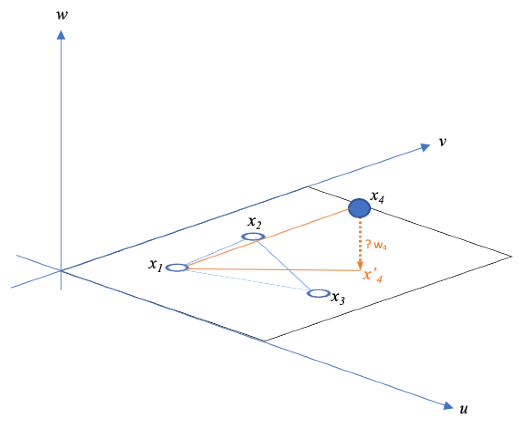
This constraint can easily be understood with the geometric representation of an example. Suppose 4 sensors. A plane is defined by three non-collinear points. As such, any set of 3 sensors and will define a plane and their distance matrix will surface 2 positive eigenvalues. Adding a fourth sensor introduces two possibilities: the additional sensor will either be on the plane (or close to it), or away from the plane (thus indicating or , and thus a three dimensional space ) as shown in Figure 2.
Thus, if we note the distance between points i and j, the component of point along the u axis, and and its components along the v and w axis respectively, it is possible that , bringing to the plane defined by and . Quite naturally, in a multi-storey building, it could also happen that , and are on different floors, forming a plane that is not parallel to the ground (and could be yet on a third floor). However, as will be seen below, this scenario does not apply in the case of FTM, as the signal from one sensor would not be detected across two floors.
However, FTM does not provide and , but and . Determining the dimension of the linear span of is congruent to computing . As , and therefore, considering a evaluated distance matrix reduced to the pair (), then the matrix obtained after double centering becomes:
And the simple resolution to U shows that:
If to inscribe onto the plane defined by , then:
And naturally:
Even if , any imprecision in the measurement of generates a dilation that is directly translated into a non-null proportional to . In an environment where vertical separation is often considerably less than horizontal separation, an unknown pairwise soon prevents the resolution of . For example, in a deployment where APs or sensors are positioned every 20 to 25 meters and floors (including slabs and isolation) are 4 meters apart, a measurement of prevents the experimenter from determining if and = 0 or if and , if cannot deterministically be determined to be 1.2 or lower.
In the case of Wi-Fi ranging, this issue is easily solved with Received Signal Strength Indicator (RSSI) evaluations and LoS path loss equations. But we postulate that time of flight techniques alone cannot solve this issue unless k is consistent across all and estimated precisely. As will be demonstrated below, such quantization and uniformization of k is possible, but the experimenter cannot know if the dilation is due to a wall or the material separating two floors.
mMDS does introduce the idea of different dilation values with several possible techniques, commonly centered around the idea of defining a cost function, often called the strain or stress function. Such function is defined for example in [19] as
where is an ideal distance set between the points i, j and k, given the observed measurement , and is a weight used to express the relative importance or precision of a given measurement . This relative importance does not aim at resolving dilation asymmetries. In fact, the resolution to U can take several iterative forms around mechanisms all aiming at minimizing the cost function . In all cases, the choice of is critical, as it can be different for each . However, in most cases, is modulated based either on confidence indices ( is high for known to be close to the ground truth) or on point criticality ( is high for i and j being anchors important to the problem to solve, e.g., connection points to other networks etc.), not on dilation asymmetries. Other MDS techniques proceed with similar logic, with the general idea that distances may be noisy, but the noise being unknown, it can be considered as Gaussian, i.e., symmetric in most directions. Regardless of the method chosen, both the minimization and the double centering techniques tend, as noted in [20], to center the points along the mean of the error, and therefore to center the error. However, in the case of FTM (and probably multiple other time-of-flight-based distance estimation techniques), the noise is not Gaussian throughout the matrix.
4.1.3. Error Averaging
This last point causes the third additional difficulty. mMDS only considers the positive eigenvalues. This is a necessary requirement of the distance-to-coordinate resolution process, which needs the coordinate U to be derived from a centered matrix B eigendecomposition ( described in the previous section). Through this process, the coordinate matrix U is found as . To maintain in R (i.e., ensure that such matrix does not have a complex part), and working on the principle that the number of eigenvalues reflects the object dimension, needs to have an expression solely in R (i.e., no complex part). This requirement means that negative eigenvalues are ignored.
However, as displayed in Table 1, real world FTM measurements typically produce through the mMDS process multiple large positive eigenvalues, but also, sometimes large, negative eigenvalues. As demonstrated in [20], B is an approximation of XX’, because it is built from , not from D. As a consequence, writing and the square of R Frobenius norm, and its trace, [20] shows that the resulting coordinates estimation error can be found to be:
This result shows that the error increases as the difference between and increases. It is also easily seen that the mMDS process centers the error. This issue can easily be seen through a simple example. Suppose a simple measured distance matrix with 3 points, each distance being affected by a specific dilation factor:
In this simple configuration:
And thus:
From B, it can clearly be seen that dilation factors that affect a single distance pair in are projected as weights for the computation of the centered matrix B, affecting all other entries of B in the process. The weights, because of the structure of J, affect differently the various pairs. The sum of the contribution of each dilation factor in B is now 1 for each row or column where the factor was present in and for each row or column where the factor was not present. Overall, the contribution in B is reflective of the overall contribution in . However, centering the matrix also has the effect of distributing the dilation factors, and thus distributing individual dilation factors.
The outcome of such distribution is that a single large dilation factor will then affect the computed position of all points in U, thus distributing the error to all positions. In a distance setting where the noise is Gaussian across all sensors, this distribution has only minor effects. However, in settings, like indoor location with FTM, where noise asymmetry is present, and where accuracy depends on identifying the RF interference localities and the associated dilation differences between pairs, mMDS, used alone, can provide an acceptable result, but that will always be worse than quality LoS measurements. As a consequence, highly dilated distance pairs get hidden in the transformation, and precise measurements get degraded by the contribution of dilated pairs.
Therefore, there is a need for a method that can identify and compensate for the highly dilated segments, to attempt to reduce their dilation before they are injected in a method, such as mMDS, where all segment contributions are treated equally.
5. Materials and Methods
5.1. First Component: Wall Remover-Minimization of Asymmetric Errors
One first contribution of this paper is a method to reduce dilation asymmetry. Space dimension is resolved using other techniques (e.g., RSSI-based), and Section 6 will provide an example. Once the dimension space has been reduced to and only sensors on the same floor, we want to reduce the dilation asymmetry. Figure 1 illustrates a typical asymmetry scenario. In this simplified representation, a strong obstacle appears between the sensor and sensors and , causing the distances , and to be appear as , and respectively. At the same time, supposing that the system is calibrated properly and LoS conditions exist elsewhere, the obstacle does not affect distance measurements between and and , that are all approximated along the same linear dilation factor k.
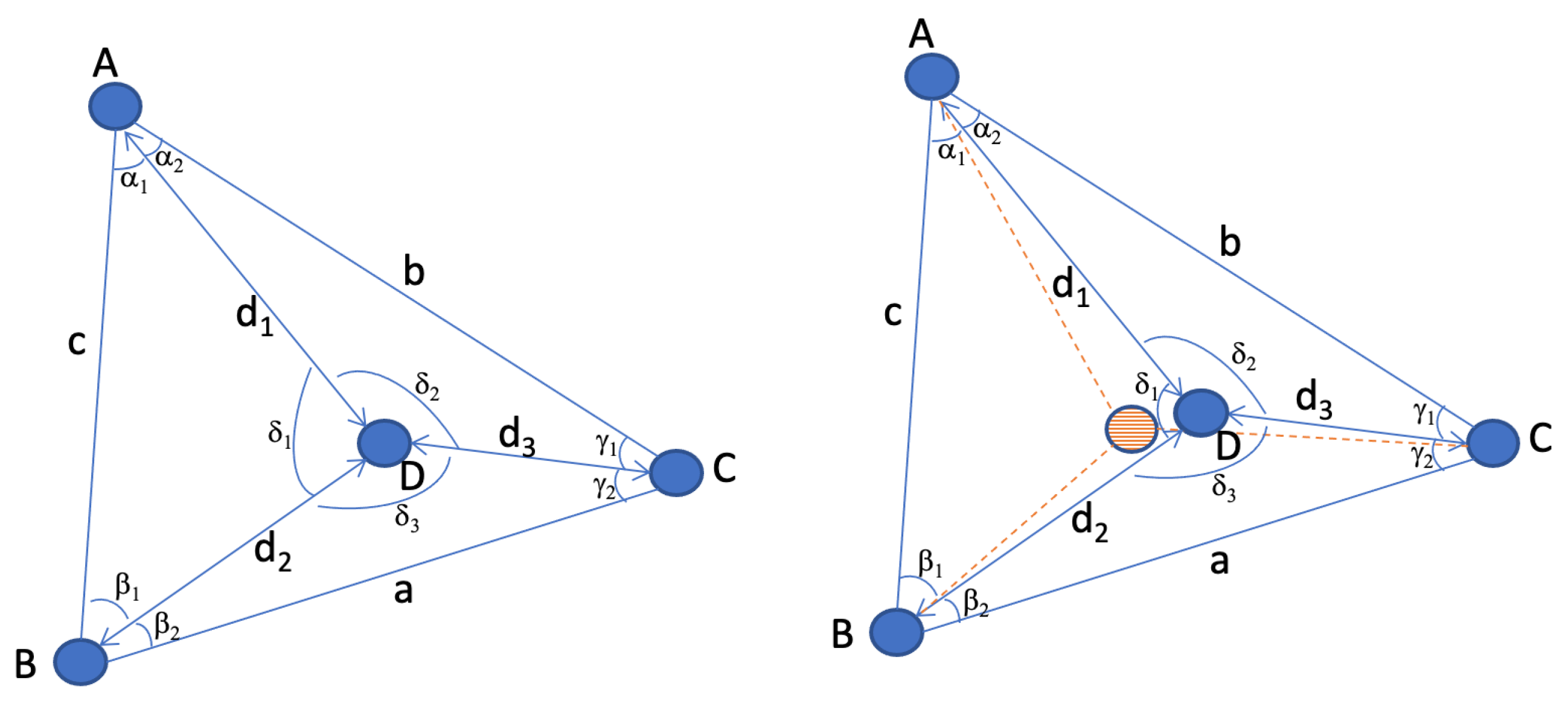
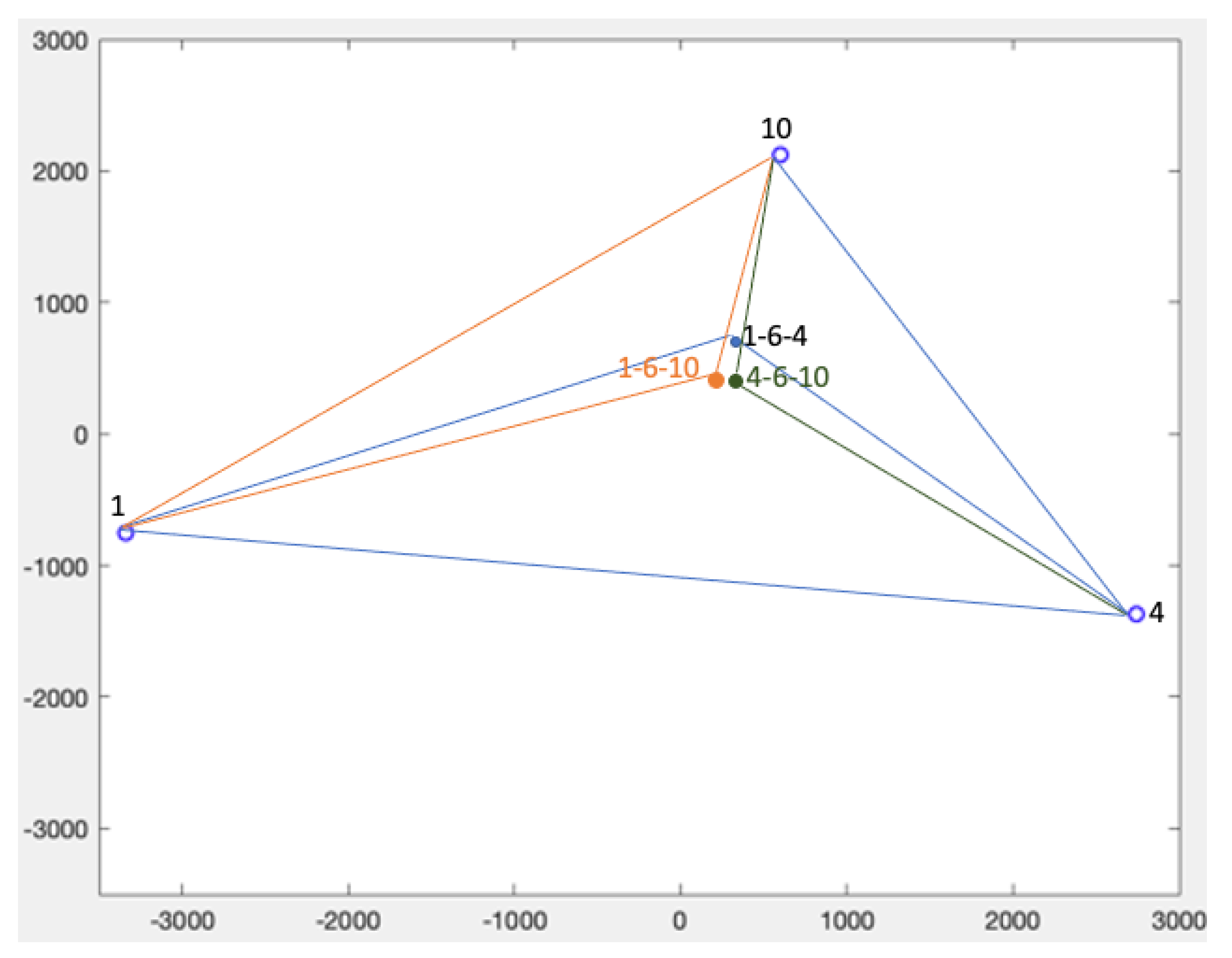
In such case, using a centering technique to average the error may make sense algebraically, but not geometrically. Finding a method to reduce the error while detecting its directionality is therefore highly desirable. Luckily, geometry provides great methods to this mean, that only have the inconvenience of requiring multiple comparisons. Such process may be difficult when performing individual and mobile station ranging, but becomes accessible when all sensors are static. When implemented in a learning machine, this method can be implemented at scale and reduce the distance error only when it is directional, thus outputting a matrix which k factor is closer to uniformity. It should be noted that the purpose of such method should not be to fully solve the MDS problem, as some pair-distances are usually not known, and the method has a limited scope (i.e., it cannot assess some of the pairs, as will be seen below). However, in many cases, sensors can be found that display interesting properties displayed on the left part of Figure 3. In this scenario, 3 sensors and are selected that form a triangle. The triangle represented in the left part of Figure 3 is scalene, but the same principle applies to any triangle. A fourth sensor is found which distance to and is less than or , thus placing within the triangle formed by .
A natural property of such configuration is that and, in any of the triangles or , one side can be expressed as a combination of the other two and of its opposite angle. For example, in can be expressed as:
The above easily allows us to find and can also be used to determine angles from known distances, for example , knowing that:
Therefore, angles and missing distances can be found from known distances. In an ideal world, properties (20) and (21) are verified for each observed triangle ( and ()). In a noisy measurement scenario, inconsistencies are found. For example, an evaluation of the triangle may be consistent with the left side of Figure 3, but an evaluation of triangle may position in the hashed representation of the right part of Figure 3. It would be algebraically tempting to resolve as the middle point between both possibilities (mean error). However, this is not the best solution. In Figure 3 simplified example, the most probable reason for the inconsistency is the presence of an obstacle or reflection source between and . If all distances are approximations, some of them being close to the ground truth and some of them displaying a larger k factor, a congruent representation of such asymmetry is that k is larger for than it is for the other segments. Quite obviously, other possibilities can be found. For example, in the individual triangle , it is possible that k is larger for the segments than it is for segments and . However, as is compared to other segments and the same anomaly repeats, the probability that the cause is an excessive stretch on increases.
As the same measurements are performed for more points, the same type of inconsistency appears for other segments. Thus an efficient resolution method is to identify these inconsistencies, determine that the distance surfaced for the affected segment is larger than a LoS measurement would estimate, then attempt to individually and progressively reduce the distance (by a local contraction factor that we call ), until inconsistencies are reduced to an acceptable level (that we call ).
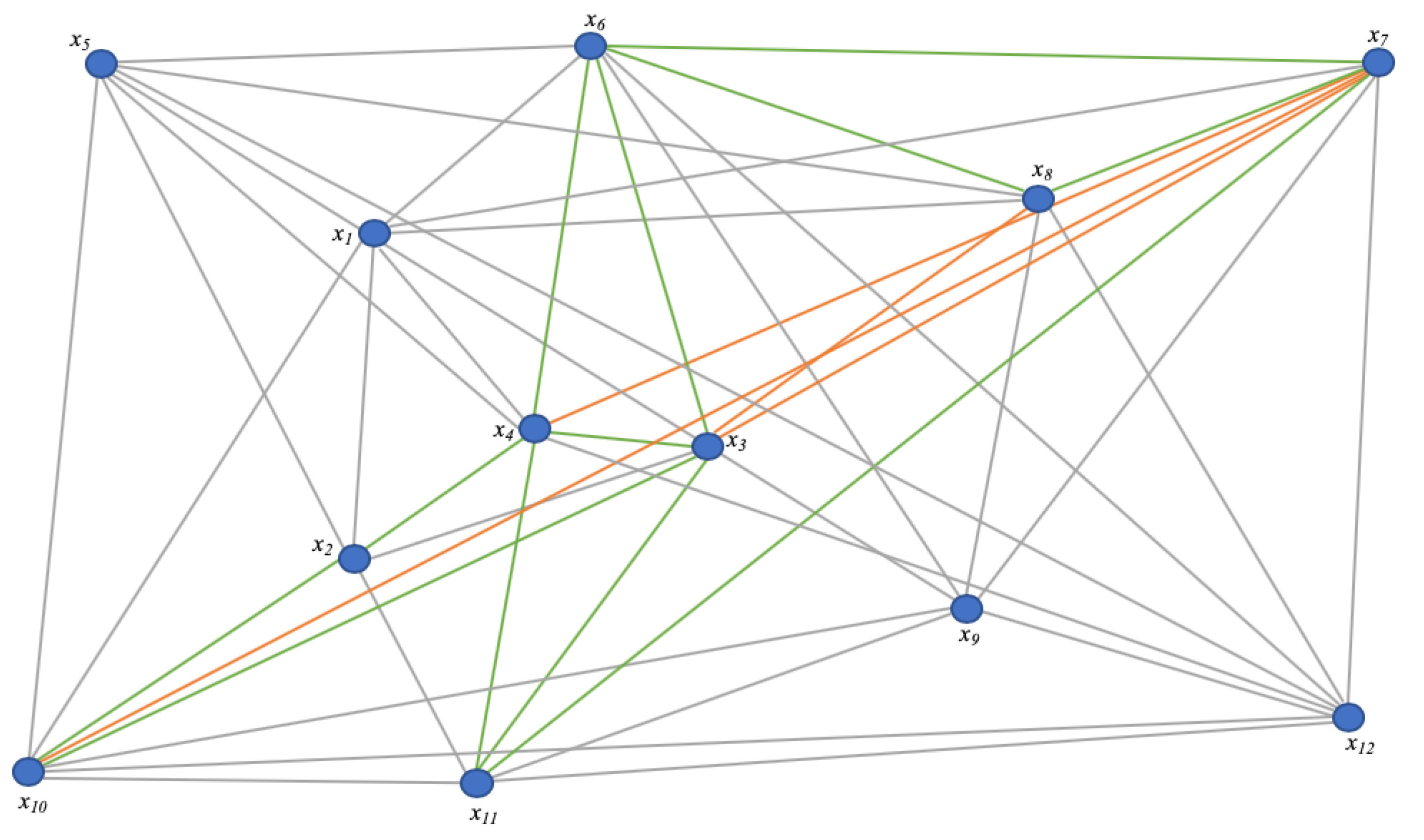
Thus, formally, a learning machine that we call a geometric Wall Remover engine, is fed with all possible individual distances in the matrix, and compares all possible iterations of sensors forming a triangle and also containing another sensor. Distance matrices do not have orientation properties. When considering for example, can be found on either side of segment , and the solution can also be a triangle in any orientation. However, adding a fourth point (), which distance to is evaluated, can constrain within the triangle. As the evaluation proceeds iteratively throughout all possible triangles that can be formed from the distance matrix, the system first learns to place the sensors relative to each other. The resulting sensor constellation can have globally any orientation, but the contributing points partially appear in their correct relative position.
Then, each time a scenario matching the right side of Figure 3 is found, the algorithm learns the asymmetry and increases the weight w of the probability p that the matching segment ( in this example) has a dilated factor (cf. Algorithm 1). As a segment may be evaluated against many others, its w may accordingly increase several times at each run. The algorithm starts by evaluating the largest found triangles first (sorted distances from large to small), because they are the most likely to be edge sensors. This order is important, because in Figure 3 example, a stretched value may cause to be graphed on the right side of segment , and thus outside of . This risk is mitigated if multiple other triangles within can also be evaluated. An example is depicted by Figure 4. In this simplified representation (not all segments are marked), the position of is constrained by first evaluating and against and . This evaluation allows the system to surface the high probability of the stretch of segment , suggesting that should be closer to than the measured distance suggests, but not to the point of being on the right side of . The system can similarly detect a stretch between points and (but not between and or and ).
| Algorithm 1: Wall Remover Algorithm |
| Input : : learning rate : acceptable error range |
| Output: optimized |
 |
At the end of the first training iteration, the system outputs a sorted list of segments with the largest stretch probabilities (largest w and therefore largest p). The system then picks that segment with that largest stretch, and attempts to reduce its stretch by proposing a contraction of the distance by an individual factor. The factor can be a step increment (similar to other machine learning algorithms learning rate logic) or can be proportional to the stretch probability. After applying the contraction, the system runs the next iteration, evaluating progressively from outside in, each possible triangle combination. The system then recomputes the stretch probabilities and proposes the next contraction cycle. In other words, by examining all possible triangle combinations, the system learns stretched segments and attempts to reduce the stretch by progressively applying contractions until inner neighboring angles become as coherent as possible, i.e., until the largest stretch is within a (configurable) acceptable range from the others.
This method has the merit of surfacing points internal to the constellation that display large k factors, but is also limited in scope and intent. In particular, it cannot determine large k factors for outer segments, as the matching points cannot be inserted within triangles formed by other points. However, its purpose is to limit the effect on measurements of asymmetric obstacles or sources of reflection.
5.2. Second Component: Iterative Algebro-Geometric EDM Resolution
The output of the wall remover method is a matrix with lower variability to the dilation factor k, but the method does not provide a solution for an incomplete and noisy EDM. Such reduction still limits the asymmetry of the noise, which will therefore also limit the error and its locality when resolving the EDM, as will be shown below. Noise reduction can be used on its own as a preparatory step to classical EDM resolution techniques. It can also be used in combination with the iterative method we propose in this section, although the iterative method has the advantage of also surfacing dilation asymmetries, and thus could be used directly (without prior dilation reduction). Combined together, these two techniques provide better result than standard EDM techniques.
EDM resolution can borrow from many techniques, which address two contiguous but discrete problems: matrix completion and matrix resolution. In most cases, the measured distance matrix has missing entries, indicating unobserved distances. In the case of FTM, these missing distances represent out-of-range pairs (e.g., sensors at opposite positions on a floor or separated by a strong obstacle, and that cannot detect each other). A first task is to complete the matrix, by estimating these missing distances. Once the matrix contains non-zero numerical values (except for the diagonal, which is always the distance and therefore always 0), the next task is to reconcile the inconsistencies and find the best possible distance combination.
Several methods solve both problems with the same algorithm and [21] provides a description of the most popular implementations. We propose a geometric method, that we call Iterative Algebro-Geometric EDM resolver (Algorithm 2), which uses partial matrix resolution as a way to project sensor positions geometrically onto a plane, then a mean cluster error method to identify individual points in individual sets that display large asymmetric distortions (and should therefore be voted out from the matrix reconstruction). By iteratively attempting to determine and graph the position of all possible matrices for which point distances are available, then by discarding the poor (point pairs, matrices) performers and recomputing positions without them, then by finding the position of the resulting position clusters, the system reduces asymmetries and computes the most likely position for each sensor.
We want to graph the position of each point in the sub-matrix. A pivot is chosen iteratively in . In the first iteration, , then in the second iteration, and in the last iteration. For each iteration, is set as the origin, and . An example is displayed in Figure 5. The next point in the matrix () is iteratively set along the x-axis, and . If , then the position of each other point of the set is found using standard triangular formula illustrated by the points in Figure 5 and where:
and
| Algorithm 2: Iterative algebro-geometric EDM resolution algorithm |
| Input: |
 |
Formally, the measured distance matrix of n sensor distances is separated in sub-matrices. Each sub-matrix contains points for which inter-distances were measured, so that:
Such formula fixes the position of above the u-axis (because is always positive). This may be ’s correct position in the sensor constellation in some cases, but can also result in an incorrect representation as soon as the next point is introduced in the graph. A simple determination of the respective positions of and can be made by evaluating their distances, as in the wall remover method. In short, if , then and are on opposite sides of the u-axis and becomes .
As the process completes within the first matrix, the position of m points are determined using the first pair of points and as the reference. In the next iteration, is kept but changes from to . Algebraically, the first iteration determines the positions based on the pairwise distances expressed in the first 2 columns of the distance matrix, while the second iteration determines the positions based on the pairwise distances expressed in the first and third columns. Both results overlap for the first 3 points and , but not for the subsequent points. This can be easily understood with an example. Recall that for any pair of points i and j, . Using as a representation of both and , and the following small matrix of 5 points as an example:
The first iteration ignores and that are represented in the second iteration (but the second iteration does not represent or ).
As in the second iteration is used as a reference point for the x axis, the geometrical representations of the first and the second iterations are misaligned. However, is at the origin in both cases, and is represented in both graphs (we note them and ). Using Equation (22), finding the angle formed by the points is straightforward, and projecting the second matrix into the same coordinate reference as the first matrix is a simple rotation of the second matrix, defined by T as:
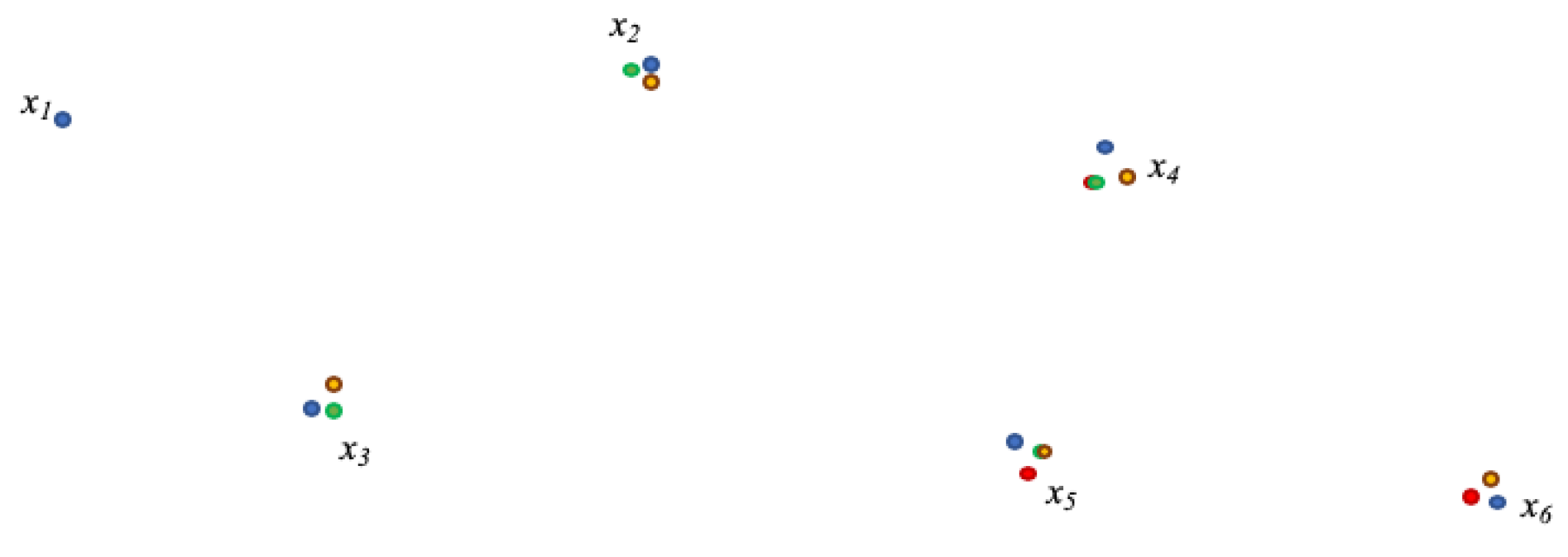
In the subsequent iterations, ceases to be at the origin. Depending on the sub-matrix and the iteration, may or may not be in the new matrix. However, 2 points and can always be found that are common to both the previous matrix and the next matrix . Projecting into the same coordinate reference as is here again trivial, by first moving the coordinates of each point found from by and then perform a rotation using Equation (22). These operations are conducted iteratively. As measured distances are noisy, for each point represented in , different coordinates appear at the end of each iteration, thus surfacing for each point a cluster of computed coordinates. Figure 6 represents this outcome after 4 iterations over a 5-point matrix and fixed about the first point.
The effect of projection and rotation makes that the red and green points are overlapping in , and the green and orange point are overlapping in . The choice to determine which points should be used to project onto is sequentially obvious, but arbitrary otherwise. In the example displayed in Figure 6, instead of could have been chosen to project iteration green onto iteration red etc. A reasonable approach could be to compute iteratively, another one to compute all possible combinations, a third approach is to compute the mean of the positions determined for a point as the best representation of the likely position of a given point for a given iteration. The second method is obviously more computationally intensive, but provides a higher precision in the final outcome. As a cluster of positions appears for each point, representing the computed position of each sensor, asymmetries and anomalies can here as well be surfaced. All points associated with a sensor form a cluster, which center can be determined by a simple mean calculation, where for each cluster center ,) and m associated points:
And
Projections that are congruent will display points that are close to one another for a given cluster. However, the graph will also display some representations that display a large deviation. This deviation can be asymmetric. It is then caused by a dilation factor k different for a sensor pair than for the others. In most cases, strong obstacles or reflection sources may increase the dilation factor. The geometric wall remover method exposed in the previous section of this work is intended to reduce such effect. As the algorithm acts on the angles of adjacent triangles, it is more precise than this section of our proposed method. However, it may happen that the dilation occurs among pairs than the geometric wall remover cannot identify (for example because the pair is formed with sensors at the edge of the constellation).
The deviation also surfaces matrices coherence. A coherent matrix contains a set of distances displaying a similar dilation factor k. An incoherent matrix contains one or more distance displaying a k factor largely above or below the others. For example, several sensors may be separated from each other by walls, but be in LoS of a common sensor, which will display a k factor smaller than the others. Such sensor is an efficient anchor, i.e., an interesting point or for the next iteration. On the other hand, some sensors may be positioned in a challenging location and display large inconsistencies when ranging against multiple other sensors. The position of these sensors needs to be estimated, but they are poor anchors for any iteration.
An additional step is therefore to identify good, medium and poor anchors and discard all distances that were computed using poor anchors. The same step can identify and remove outliers pairwise computed positions that deviate too widely from the other computed positions for the same points), and thus accelerate convergence. For each cluster i of m points for a given sensor, each at an Euclidian distance from the cluster center , a mean distance to the cluster center can be expressed as:
where thus expresses the mean radius of the cluster. By comparing radii between clusters, points displaying large values are surfaced. Different comparison techniques can be used for such comparison. We found efficient the straightforward method of using the rule, where a cluster which radius is more than 2 standard deviations larger than all clusters mean radii is highlighted as an outlier. The associated sensor therefore displays unusually large noise in its distance measurement to the other sensors, and is therefore a poor anchor. Matrices using this sensor as an anchor are removed from the batch and clusters are recomputed without these sensors’ contribution as anchors. As the computation completes, each cluster center is used as the best estimate of the associated sensor position. By reducing the variance of the dilation factor k, by removing sub-matrices and sensor pairs that bring poor accuracy contribution, this method outperforms standard EDM completion methods when is known, because it reduces asymmetries before computing positions, but also because the geometric method tends to rotate the asymmetries as multiple small matrices are evaluated, thus centering the asymmetries around the sensor most likely position.
6. Results
6.1. Experiment Methodology
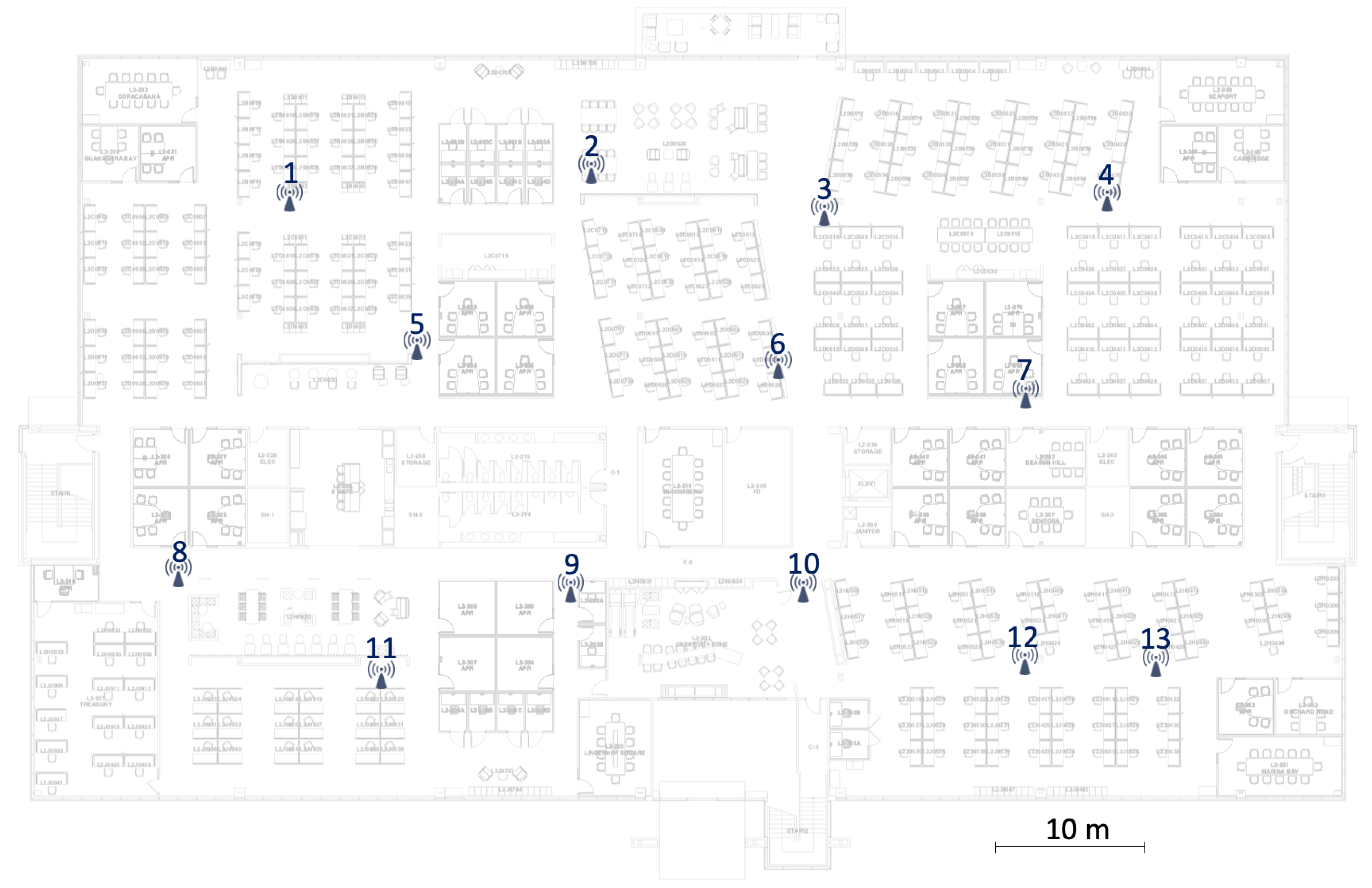
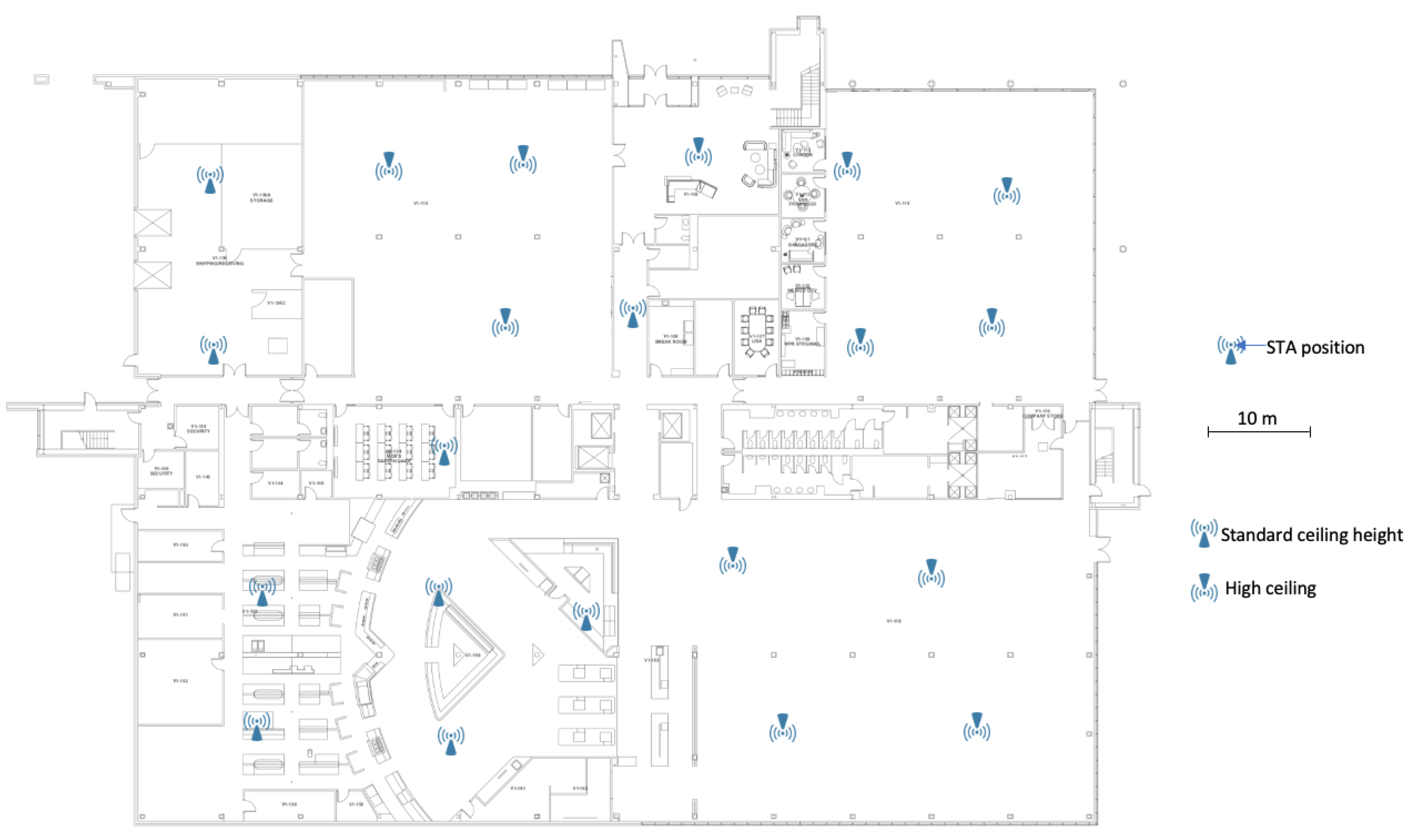
We tested this method in five different buildings already equipped with Wi-Fi APs providing active coverage. As the active APs do not support FTM, we position FTM devices near each active AP (typically 15 cm, of half a foot, from each active AP position). Building 1 is a three-storey office building with cubicle areas alternating with blocks of small offices. Our testbed is installed on the second floor. Building 1 is interesting, because the wall structure is irregular, causing different reflection and absorption patterns for each AP pair. The test floor is already equipped with 13 access points positioned at ceiling level. We therefore positioned 13 FTM stations at ceiling level, one near each AP, as represented in Figure 7.
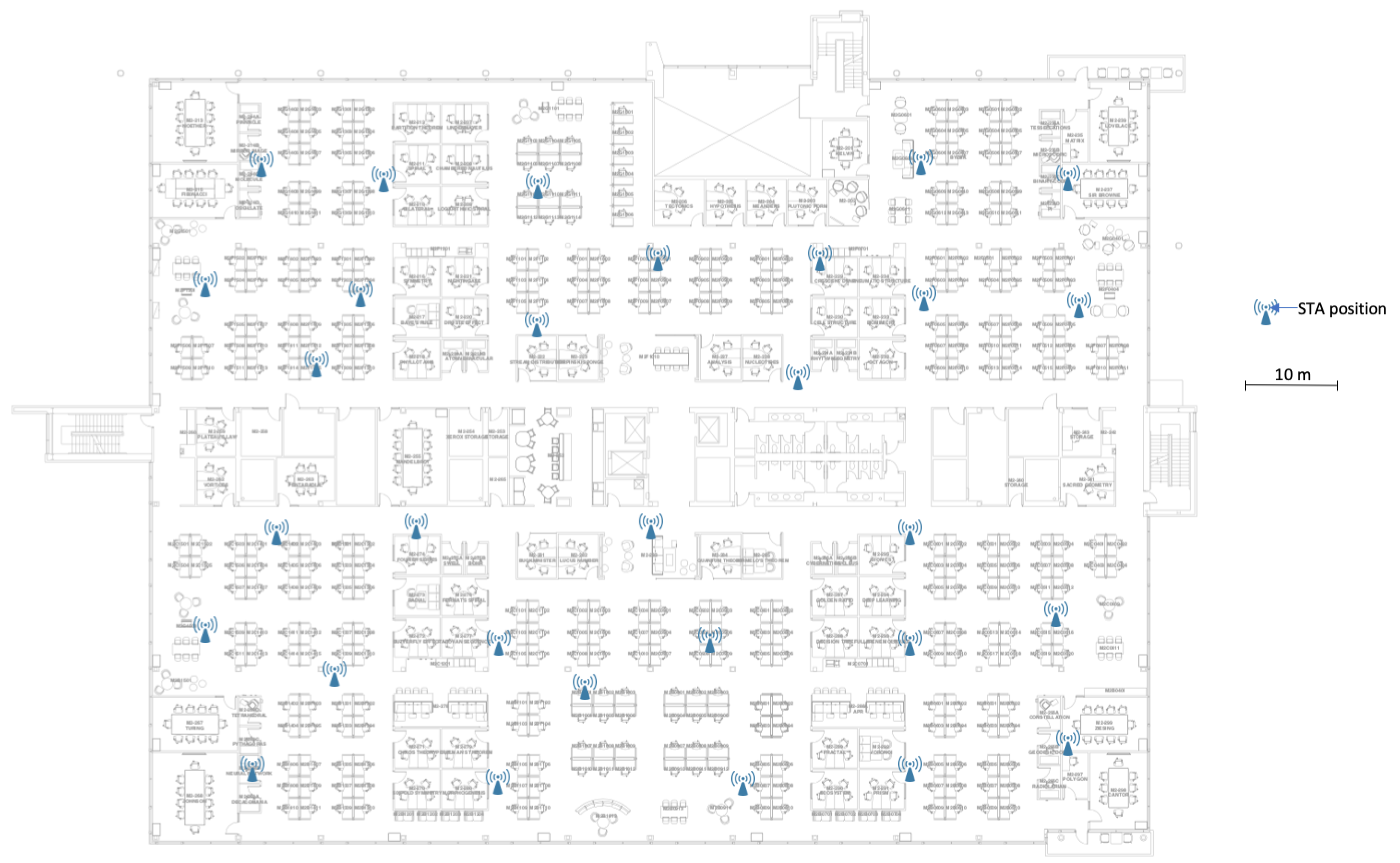
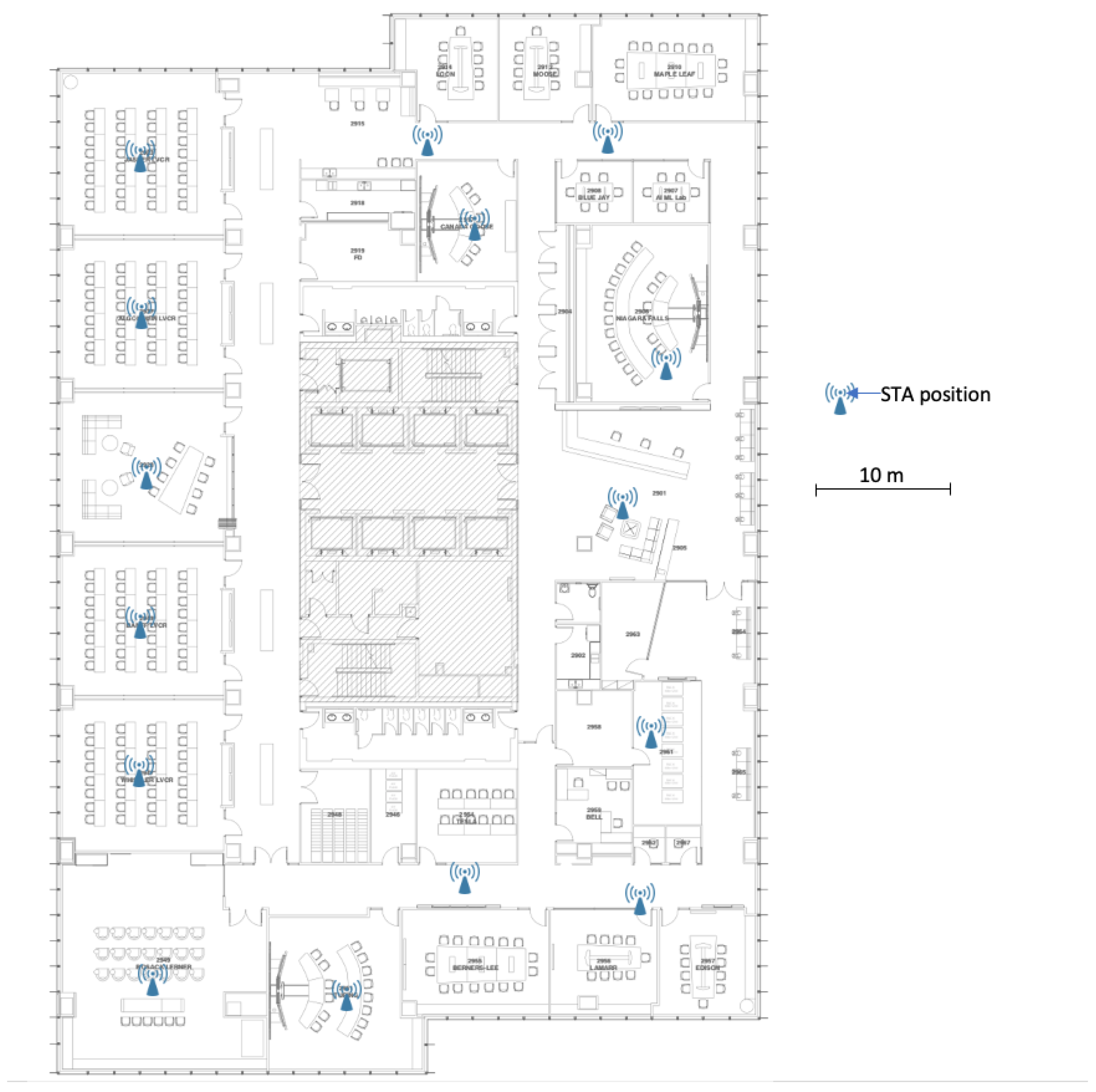
Building 2 is also an office building with 30 APs, with denser sitting density than building 1 and where zones of open space alternate with strong obstacles. Similarly to building 1, one FTM device is positioned 15 cm (1/2 foot) away from each existing AP, as represented in Figure 8.
Building 3 is a large open space building with partial high ceilings, used as an enterprise restaurant. It presents high peaks of user and Wi-Fi traffic alternating with no activity. This traffic pattern allows us to evaluate the effect of traffic (or lack thereof) on ranging accuracy. Additionally, the building structure makes that AP height is not consistent throughout the floor, thus presenting an interesting geometry. Building 3 is represented in Figure 9. High-ceiling APs are represented by upside down icons. In this setting, all APs are the same model and use omnidirectional antennas. Thus, the only difference between APs is their height, 3.2 meters for standard ceiling heights, and 7.3 meters for high ceiling APs. Our FTM devices are positioned near each AP as in the previous buildings.
Building 4 is a warehouse, with metallic racks, high ceilings and some APs mounted with directional antennas. An office space is present in the upper right corner of the building. High ceiling APs use omnidirectional antennas and are positioned on poles hanging from the ceiling, between 6.4 and 8.1 meters above the ground. On the side of the aisles, some APs are mounted at 3.4 meters height and equipped with directional patch antennas, as represented in Figure 10. For our experiments, we use these antennas to evaluate the effect of directionality.
Building 5 is a training center with small to medium-sized classrooms. It presents an interesting denser wall structure (as walls separate the classrooms). As represented in Figure 11, each classroom has its own AP in the center. The dense (hashed) non-accessible technical area at the center makes that APs on one side do not detect APs on the other side.
For the main presentation of this section, we will focus on building 1 as the main example, and will highlight the other buildings when they present interesting variations. In all cases, our FTM devices are Linux systems equipped with Intel 8260 cards enabled for FTM. In the rest of this section, we will refer to AP-to-AP distances and measurements, although it should be clear that the FTM device associated to each AP was used to operate the measurement. Ground truth distances are known and confirmed with floorplan blueprint and onsite laser ranging. The FTM devices can be configured to act as ISTAs or RSTAs. The system is left active for two days (with the exception of the warehouse, where the system is left active for 6 hours, so as to minimize the disruptions to the warehouse operations). Every hour, the system wakes up, and each station is randomly affected the role of ISTA or RSTA. Each ISTA ranges against the detected RSTAs on various channels for 10 minutes and logs the result. At the end of the collection phase, the logs of all stations are collected and injected into the learning machine.
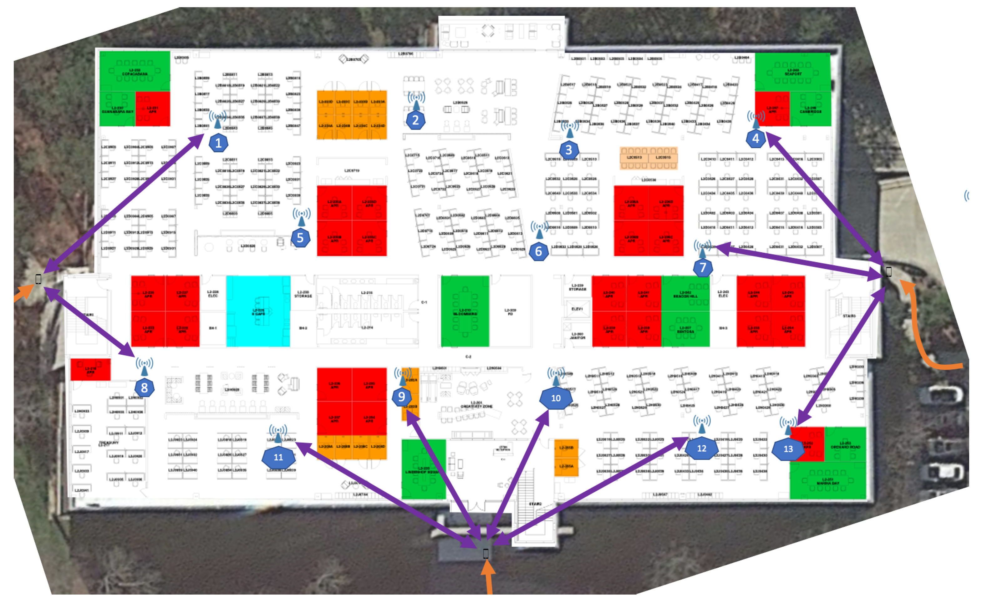
This duration was chosen to ensure that collection would happen both at quiet times (at night, with no user is in the building) as well as during busy day times. Although daytime measurements do show larger collision and retry counts, no significant difference could be observed in ranging accuracy. It is therefore likely that the system could only be left active for a shorter duration and yet obtain convergence. Mobile stations are also walked around the building, to determine locations where ranging to indoor APs would be possible. From left entrance and stairs, APs 01, 08 and 11 are reachable. From the main entrance (bottom), APs 11, 09, 10 12 and 13 are reachable. From the right entrance and stairs, APs 13, 07 and 04 are reachable as can be seen in Figure 12.
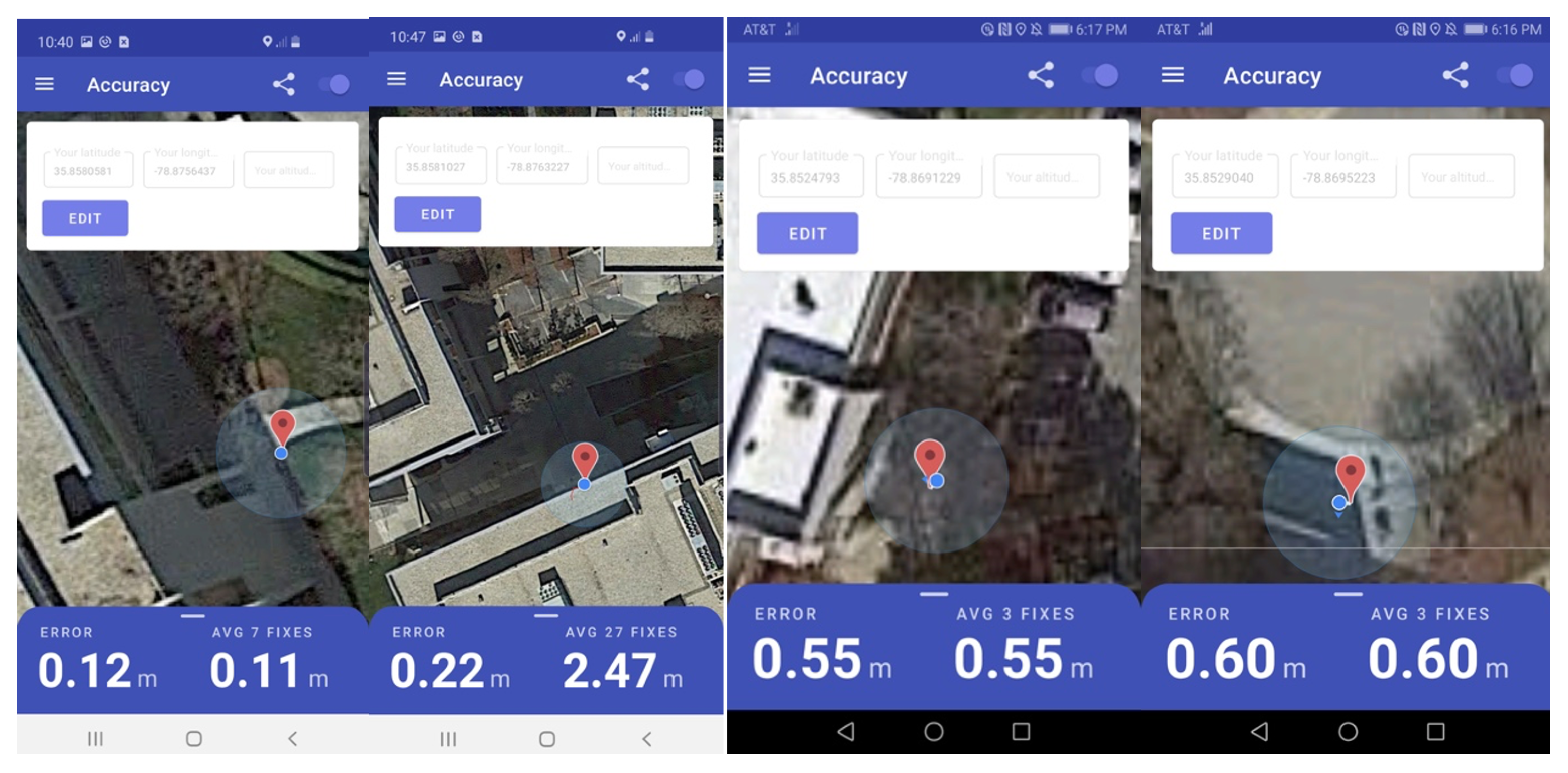
The purpose of the outdoor mobile stations is to serve as a seed for an initial GPS position communicated to the APs in range of the station. One key determinator is the accuracy of the GPS value seeded by the mobile station. GPS accuracy utilities are installed on different phones. As GPS position is computed, the operator clicks the real location, based on high resolution aerial maps, and the system outputs the error of the computed GPS estimation. As displayed in Figure 13, the error is commonly within half a meter. Inside the building, accuracy collapses (not represented here).
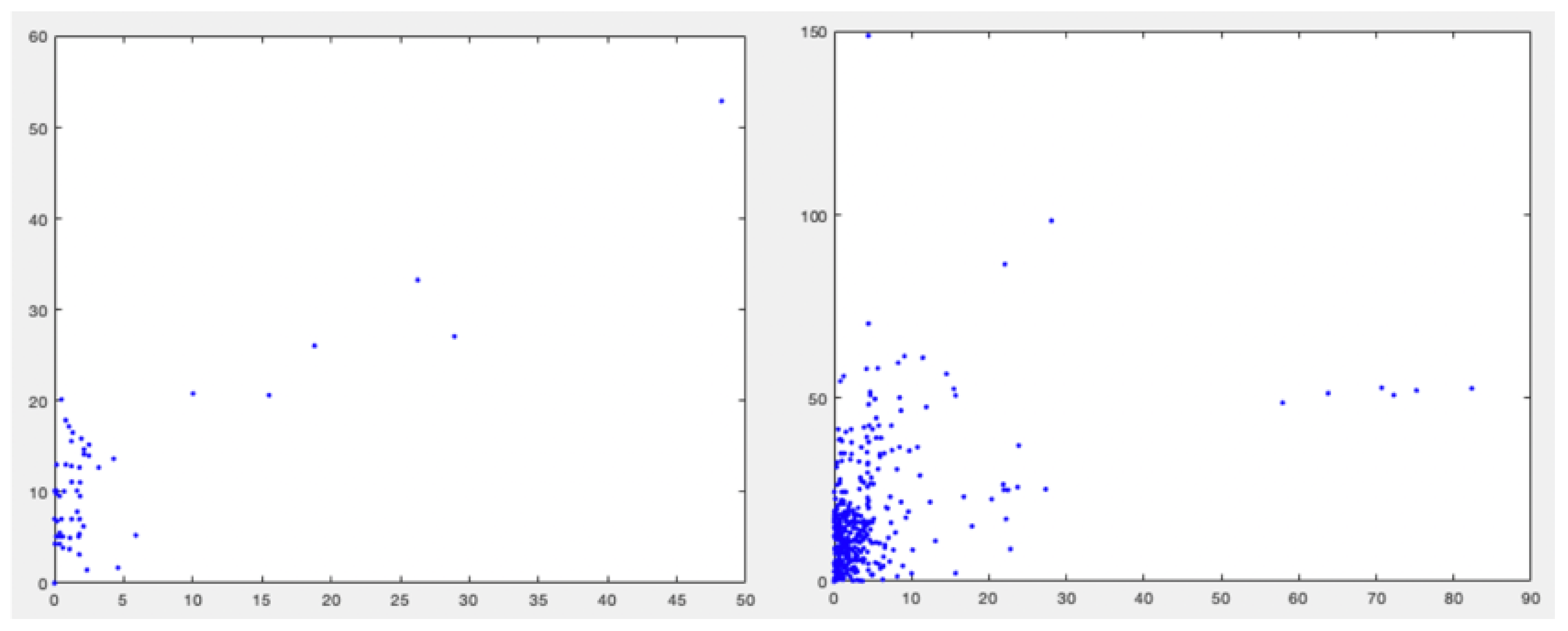
An examination of the distance matrix for all APs (measured through their associated FTM devices) shows high noise. Table 1 displays the ground truth (real distances) and Table 2 the distances obtained via FTM measurements, after applying the simplification. The ground truth matrix surfaces 9 positive eigenvalues, because measurements suffered from natural scale and rounding inaccuracies. However, only 2 of these eigenvalues are large, indicating a 2-dimensional geometrical object. The measured FTM matrix, on the other hand, surfaces ‘only’ 7 positive eigenvalues, but all of them are large. The first two eigenvalues are larger by a factor of 10 compared to the others, but this factor is not sufficient to discount the other 5 large positive eigenvalues.
The measured FTM matrix generated from the other buildings present the same type of difficulty. Building 2 (also office building, but with 30 APs), the matrix surfaces 9 large eigenvalues. In building 3 (restaurant with partial high ceiling), 6 large positive eigenvalues are seen, obfuscating the fact that the deployment is three-dimensional. In building 4 (partial high ceiling warehouse), 11 large engeinvalues are seen. In building 5, 3 large eigenvalues are seen (while all the APs are on the same plane). This last observation may be caused by the strong obstacle in the center of the building, which reduces the number of measurable distances (although 14 APs are deployed, no AP/ FTM device has measurable distance to more than 8 other APs (FTM devices); i.e., throughout the matrix each AP has no measured distance to 8 to 11 APs). As such, it is clear that the distance matrix alone is not sufficient to assert the dimensionality of the space. However, complementing with RSSI evaluation easily solves the issue. In building 1, another AP (AP15) is positioned on the upper floor, above AP05, and another (AP16) above AP06. As the ISTAs and RSTAs exchange at constant power (20 dBm), and although the RSSI is an inaccurate representation of the received power, a simple linearization and comparison between the distance computed by FTM and the expcted signal (in free path) at that distance shows that AP15 signal to any AP systematically appears 12 to 28 dB below the pairwise signal between these APs at equivalent distance. By contrast, AP16 to AP15 signal appears 10 to 25 dB above the signal from AP16 to AP01 or AP07. This result immediately indicates that AP15 and AP16 are on different floor from the others (and that both AP15 and AP16 are on the same floor). The same logic is applicable to the other buildings.
6.2. Geometric Wall Remover Phase
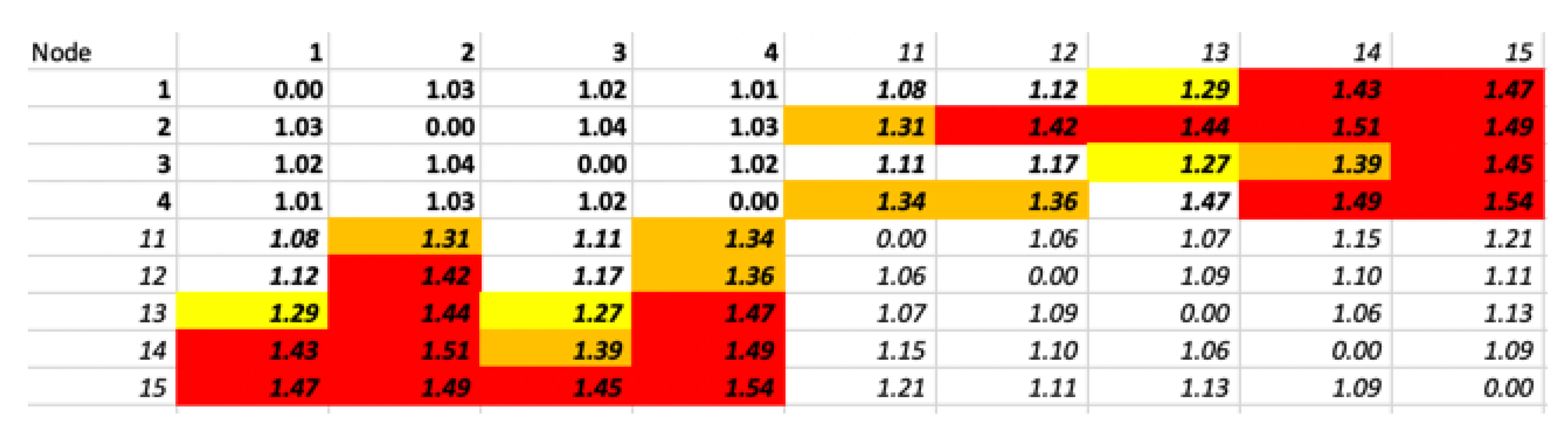
Table 3 displays the ratio between the mean of the measured distance and the ground truth in building 1. Highlighted in yellow, orange and red the distances that the geometric wall remover engine identifies as deviating from the others (small, medium or large identified deviation, respectively). Some devices are out of range from one another (e.g., device 1 against sensor 13) and are not addressed in this phase.
As can be seen, the geometric wall remover engine correctly identifies most incorrect distances, except those affecting devices positioned at the edge of the floor. A geometric illustration of this detection is represented in Figure 14, where stretches on AP6 position are detected through measuring its distance to APs 1, 4 and 10.
At the scale of the entire floor, the method initially identified pairs highlighted in red and orange in Table 3. A contraction factor was applied to each of these outliers (the step value of was chosen to be static and small, set to 0.98). As more iterations were run, each with an additional applied to identified distance dilations, the yellow pairs surfaced as abnormal. On the last iteration, the engine did not surface any more outlier, and the largest deviation from the ground truth (for the flagged pairs) was brought down to 1.13. This validation indicates that the geometric wall remover can correctly identify inner outliers and reduce the associated error, without distorting the graph (over or under reduction).
Comparable display is visible in the other buildings. FTM devices near APs on high ceiling display large distance stretches when ranging against devices near APs on lower ceilings, but devices at the edge of both domains display LoS distances and link both domains. The Geometric Wall Remover correctly identifies the high ceiling / low ceiling distant pairs as stretched, which a subset is illustrated in Figure 15. Here as well, highlighted in yellow, orange and red the distances that the geometric wall remover engine identifies as deviating from the others (small, medium or large identified deviation, respectively). High ceiling APs are 1 to 4, APs in low ceiling are 11 to 15, in italic.
6.3. Iterative Algebro-Geometric Phase
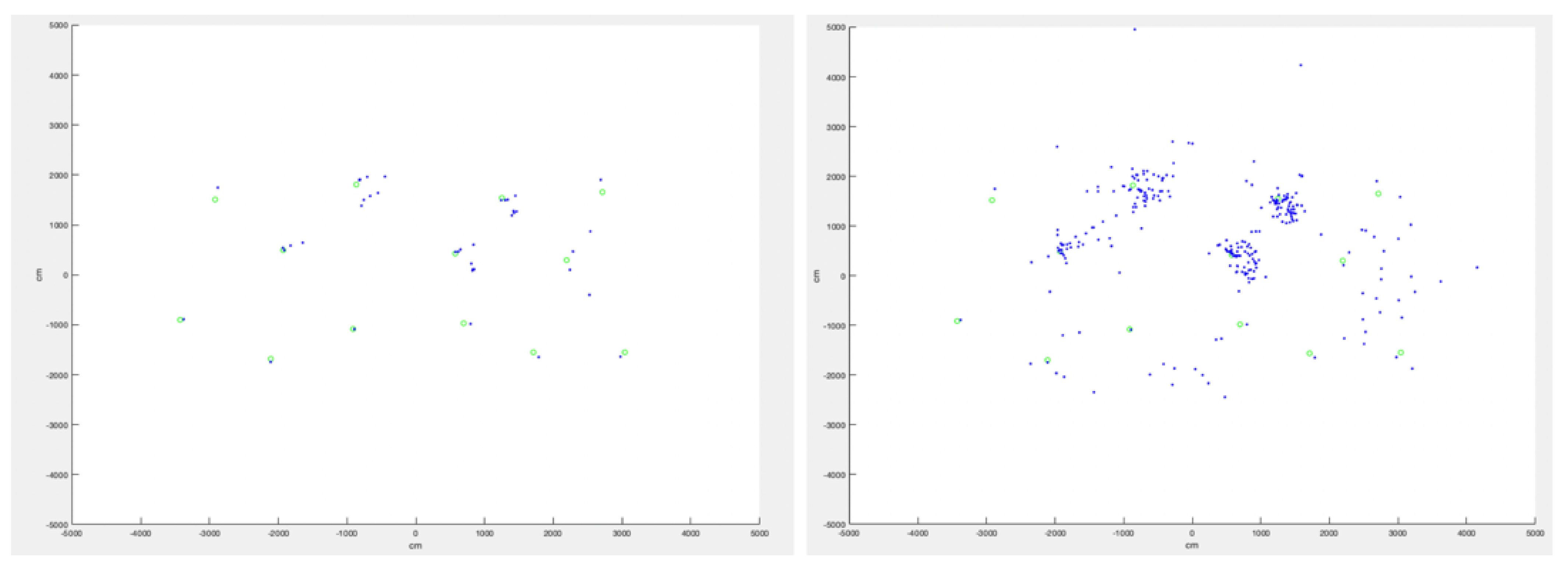
In this phase, we start with the largest possible matrix. Building 1 has 13 APs and FTM devices, and with missing distance pairs (out-of-range APs), the system iteratively finds that a matrix of size 9 starts allowing for multiple usable solutions to appear with different individual pivots, as displayed in Figure 16 (left).
Some points are used as pivots for all combinations in this iteration (and thus display a single position). As the matrix size decreases, more combinations appear. As the pivots change, noise also appears, as is visible in Figure 16 right, displaying the output of a matrix of size 8.
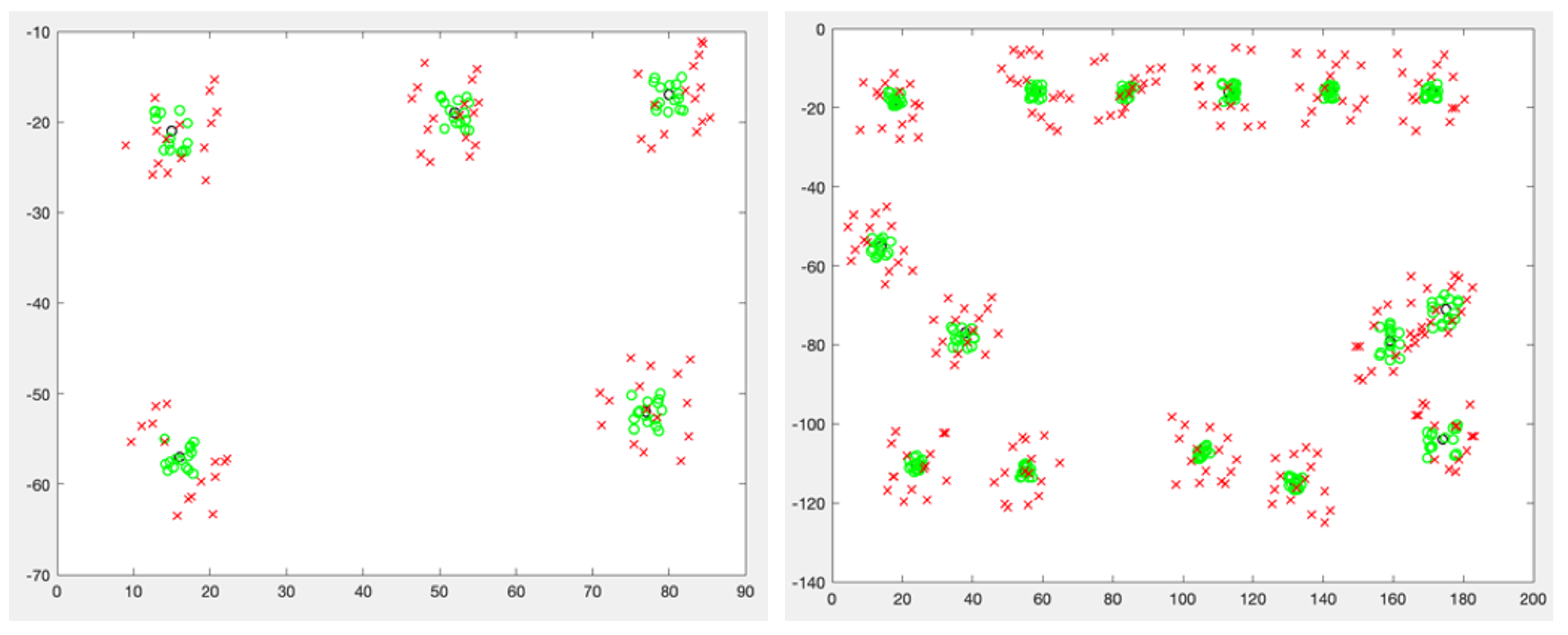
The process repeats iteratively. With smaller matrices and more combinations, clusters start to appear for each sensor, with various densities. In buildings 3 and 4, APs and devices in individual zones (low ceiling or high ceiling) are in LoS condition to each other. This is visible in Figure 17 (left), where a subset of building 3 is displayed (APs in the upper left part of the building). Green circles represent LoS (same height) matrices, while red crosses represent matrices with cross-height distances. The same density difference can be seen in building 5 (Figure 17 right), where APs/devices on the same side of the central block display close measurements (narrow clusters) while measurements through the block, when they succeed, display large variations (larger clusters).
Therefore, for any cumulated graph, cluster centers can be defined and the mean cluster radius compared between clusters. Then, outliers (points more than away from the cluster center) can be removed from each cluster, not only within each cluster individually, but also for individual pairs, where deviation from the mean pair distance can be used to identify matrix combinations that surface large individual error. As a matrix of size m is used to compute positions, the position for each device is compared through each iteration, and the difference between the coordinates found at each iteration can be graphed, as shown in Figure 18 for building 1. As the matrix size gets smaller, the noise increases, and so do deviations between computed positions, as can be seen on the right side of Figure 18. We found that starting from matrices as large as possible was computationally more efficient (as there are less large matrix combinations than small matrix combinations), and that accurate location was found with matrix of 6 or more for building 1. Smaller matrices only marginally improved the results, and the computation cost increased. The same logic was observed for the other buildings, where matrices containing at least half the floor devices (or more) produced better results.
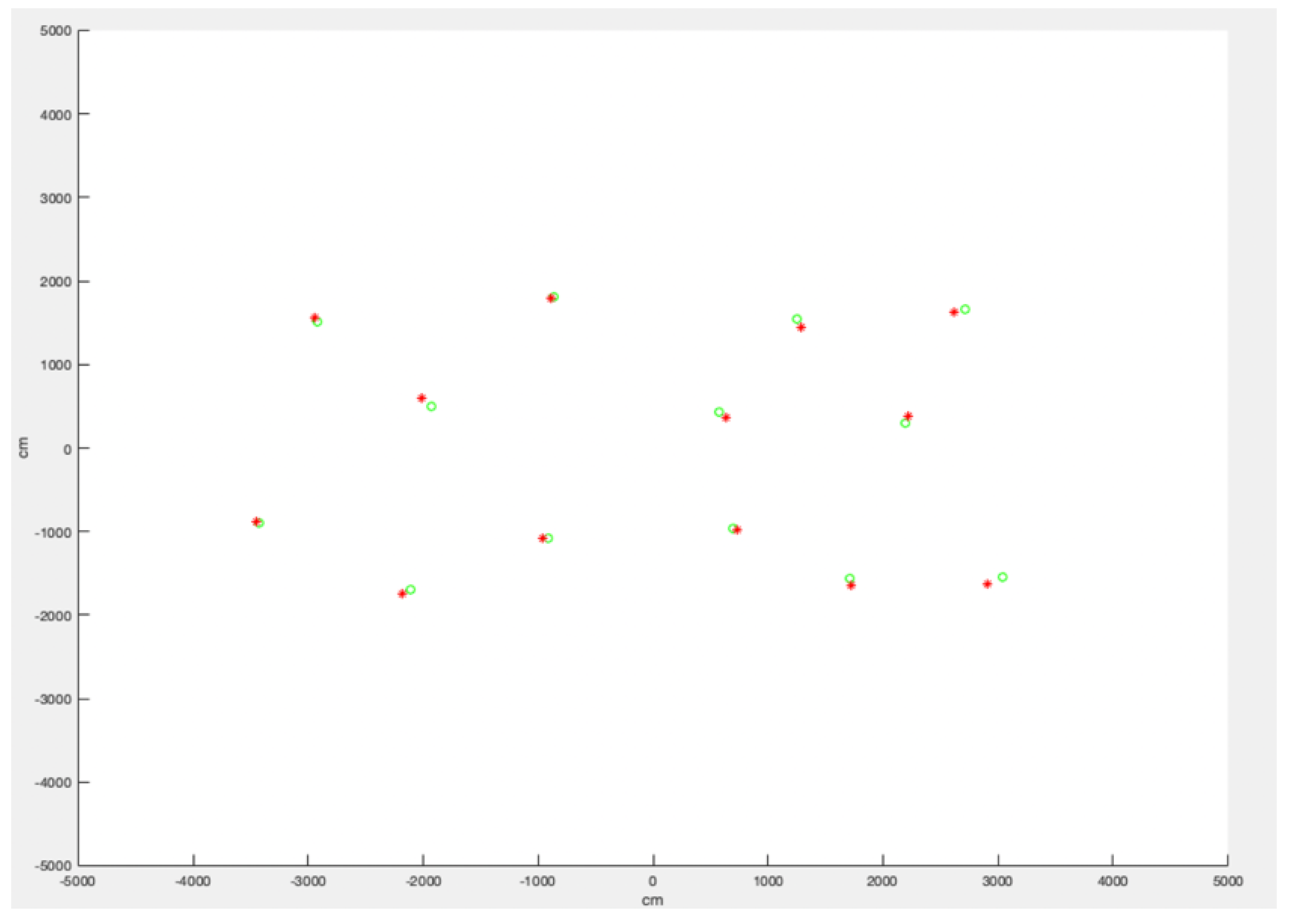
After removing the outliers, each cluster center is re-computed. The final cluster centers are displayed in Figure 19. Ground truth positions are green circles, the computed cluster position for each device is represented as a red star. The maximum error is observed at 1.1143 meter in building 1, 1.2194 meter in building 2, and 0.9621 meter in building 5. In building 3 and 4, error is small in areas at the same height (0.7304 meter and 0.6812 meters respectively). When treating the APs / devices at different height as different floor levels, this result can be sufficient to move on to the next phase.
At this stage, the relative device positions are estimated, but their orientation is not known. However, using the ranging information from one or more mobile phones, walking outside the building, to two or more FTM devices, and sending to the device the GPS location of the mobile phone as seed, the graph can be rotated to its correct orientation and the phone GPS location can be used to populate the LCI values of all devices on the graph (and therefore all APs).
6.4. Comparison with Other Methods
Noisy EDM completion is a complex problem that has been explored in multiple contexts. We will limit our comparison to the main methods listed in [21]. Naturally, using classic MDS boils down to performing an eigenvalue decomposition and geometric centering. As the matrix is noisy, the error is large. Additionally, the algorithm interprets missing distances as 0 values, which introduces irreconcilable inconsistencies in the matrix in all dimensions. The effect is worsened when the projection is constrained into . This affect can be attenuated by constructing and overlapping partial matrices for which distances are known [22]. Even in this case, the effect of asymmetry can be dire.
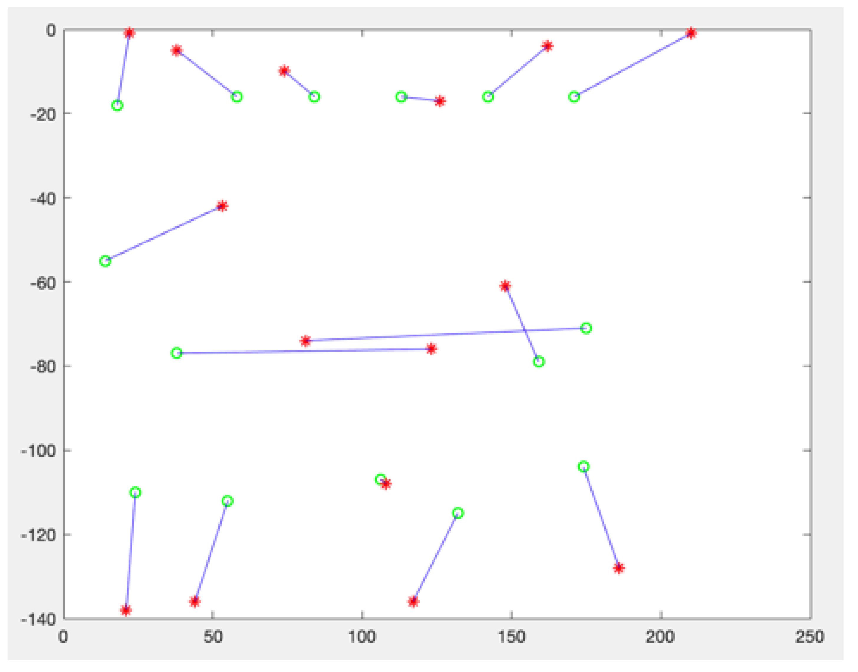
Many optimizations methods aim at finding missing elements from a matrix, but that is assumed to be noiseless. This assumption is necessary to maintain convexity, with the consequence of being unusable in our scenario. For incomplete and noisy matrices, a classical solution is to use semidefinite relaxation. This technique has multiple variants to adapt to different matrix sizes or sparsity scenarios, and both [22] and [23] are typical illustration of the associated reasoning. In all cases, the goal is to bound the rank of the Gram matrix to the target dimension space, thus constraining the number of positive and non-null eigenvalues. The process is efficient, especially for large matrices. As it proceeds iteratively, it also has the virtue of minimizing the error. In buildings where measurements errors are averaged over a large number of APs/FTM devices, the error may also be simplified to Gaussian. However, FTM works with a limited number of devices, making the limitation obvious. When the stretch is asymmetric, the error reaches a point where the method is not usable anymore. Building 5 is a typical example, where a strong obstacle is in the middle of the block, while light walls do not prevent the signal from reaching the neighboring classes. The result of classical MDS projection for this building is visible in Figure 20.
7. Conclusions
We presented a method to solve noisy Euclidian distance matrices (EDM). We showed that in the case of sensor time-of-flight measurements, measured distances are dilations of ground truth distance, but that the dilations are asymmetric, thus rendering classical EDM methods generally inaccurate, as they tend to assume noisy symmetry and therefore tend to center the error. We propose a machine learning method for identifying and reducing noise asymmetry based on evaluation of angles within overlapping triangles. We then propose a second machine learning method, aimed at graphing the positions of sensors derived from distance sub-matrices, and at identifying and removing combinations that surface excessive distances, thus progressively removing edge asymmetries and reducing the distance errors. We show that this method outperforms standard EDM resolution methods.
Author Contributions
Conceptualization, J.H., I.H.; methodology, J.H., I.H.; software, J.H., I.H.; validation, J.H., R.L., Y.B.; formal analysis, J.H., R.L.; investigation, J.H.; data curation, I.H.; writing—original draft preparation, J.H.; writing—review and editing, Y.B., R.L., N.M.; visualization, J.H., I.H.; supervision, N.M.; project administration, N.M.; funding acquisition, J.H. All authors have read and agreed to the published version of the manuscript.
Funding
This research received no external funding.
Data Availability Statement
Authors can confirm that all relevant data are included in the article.
Conflicts of Interest
The authors declare no conflict of interest.
References
- Wireless LAN Medium Access Control (MAC) and Physical Layer (PHY) Specification. 2016. Available online: https://0-standards-ieee-org.brum.beds.ac.uk/standard/802_11-2016.html (accessed on 11 March 2021).
- Yue, Y.; Ruizhi, C.; Liang, C.; Guangyi, G.; Feng, Y. A Robust Dead Reckoning Algorithm Based on Wi-Fi FTM and Multiple Sensors. Remote Sens. 2019, 11, 504. [Google Scholar] [CrossRef] [Green Version]
- Dvorecki, N.; Bar-Shalom, O.; Banin, L.; Amizur, Y. A Machine Learning Approach for Wi-Fi RTT Ranging. In Proceedings of the 2019 International Technical Meeting of The Institute of Navigation, Reston, VA, USA, 28–31 January 2019; pp. 435–444. [Google Scholar] [CrossRef]
- Polk, Y.; Linser, M.; Thomson, M.; Aboba, B. Dynamic Host Configuration Protocol Options for Coordinate-Based Location Configuration Information. Available online: https://tools.ietf.org/html/rfc6225 (accessed on 11 March 2021).
- Henry, J.; Montavont, N.; Busnel, Y.; Ludinard, R.; Hrasko, I. Sensor Self-location with FTM Measurements. In Proceedings of the 2020 16th International Conference on Wireless and Mobile Computing, Networking and Communications (WiMob), Thessaloniki, Greece, 12–14 October 2020; pp. 1–6. [Google Scholar] [CrossRef]
- Lee, L.; Jones, M.; Ridenour, G.S.; Bennett, S.J.; Majors, A.C.; Melito, B.L.; Wilson, M.J. Comparison of Accuracy and Precision of GPS-Enabled Mobile Devices. In Proceedings of the 2016 IEEE International Conference on Computer and Information Technology (CIT), Nadi, Fiji, 8–10 December 2016; pp. 73–82. [Google Scholar] [CrossRef]
- Liu, X.; Nath, S.K.; Govindan, R. Gnome: A Practical Approach to NLOS Mitigation for GPS Positioning in Smartphones. In Proceedings of the 16th Annual International Conference on Mobile Systems, Applications, and Services, Munich, Germany, 10–15 June 2018. [Google Scholar]
- Ma, L.; Zhang, C.; Wang, Y.; Peng, G.; Chen, C.; Zhao, J.; Wang, J. Estimating Urban Road GPS Environment Friendliness with Bus Trajectories: A City-Scale Approach. Sensors 2020, 20, 1580. [Google Scholar] [CrossRef] [PubMed] [Green Version]
- Mun, S.; An, J.; Lee, J. Robust Positioning Algorithm for a Yard Transporter Using GPS Signals with a Modified FDI and HDOP. Int. J. Precis. Eng. Manuf. 2018, 19, 1107–1113. [Google Scholar] [CrossRef]
- Zhao, C.; Wang, B. A UWB/Bluetooth Fusion Algorithm for Indoor Localization. In Proceedings of the 2019 Chinese Control Conference (CCC), Guangzhou, China, 27–30 July 2019; pp. 4142–4146. [Google Scholar] [CrossRef]
- Wang, P.; Luo, Y. Research on WiFi Indoor Location Algorithm Based on RSSI Ranging. In Proceedings of the 2017 4th International Conference on Information Science and Control Engineering (ICISCE), Changsha, China, 21–23 July 2017; pp. 1694–1698. [Google Scholar] [CrossRef]
- Dattorro, J. Convex Optimization Euclidean Distance Geometry 2e; Meboo Publishing: Palo Alto, CA, USA, 2019; ISBN 9780578161402. [Google Scholar]
- Zhang, K.; Shen, C.; Zhou, Q. A combined GPS UWB and MARG locationing algorithm for indoor and outdoor mixed scenario. Clust. Comput. 2019, 22, 5965–5974. [Google Scholar] [CrossRef]
- Kjærgaard, M.B.; Blunck, H.; Godsk, T.; Toftkjær, T.; Christensen, D.L.; Grønbæk, K. Indoor Positioning Using GPS Revisited. Int. Conf. Pervasive Comput. 2010, 2010, 38–56. [Google Scholar]
- Liberti, L. Distance Geometry and Data Science. TOP 2020, 28, 271–339. [Google Scholar] [CrossRef]
- Eren, T. Rigidity, computation, and randomization in network localization. IEEE Infocom. 2004, 4, 2673–2684. [Google Scholar]
- Doherty, L.; Pister, K.S.J.; Ghaoui, L.E. Convex position estimation in wireless sensor networks. In Proceedings of the Twentieth Annual Joint Conference of the IEEE Computer and Communications Society, Anchorage, AK, USA, 22–26 April 2001; pp. 1655–1663. [Google Scholar]
- Jacobs, D. Multidimensional Scaling: More Complete Proof and Some Insights Not Mentioned in Class. 2016. Available online: http://www.cs.umd.edu/~djacobs/CMSC828/MDSexplain.pdf (accessed on 11 March 2021).
- de Leeuw, J. Applications of Convex Analysis to Multidimensional Scaling. 2005. Available online: https://escholarship.org/uc/item/7wg0k7xq (accessed on 11 March 2021).
- Tsang, J.; Pereira, R. Taking All Positive Eigenvectors Is Suboptimal in Classical Multidimensional Scaling. arXiv 2016, arXiv:abs/1402.2703. [Google Scholar] [CrossRef] [Green Version]
- Dokmanic, I.; Parhizkar, R.; Ranieri, J.; Vetterli, M. Euclidean Distance Matrices: Essential theory, algorithms, and applications. IEEE Signal Process. Mag. 2015, 32, 12–30. [Google Scholar] [CrossRef] [Green Version]
- Candes, E.; Plan, Y. Matrix Completion With Noise. Proc. IEEE 2010, 98, 925–936. [Google Scholar] [CrossRef] [Green Version]
- Guo, X.; Chu, L.; Sun, X. Accurate Localization of Multiple Sources Using Semidefinite Programming Based on Incomplete Range Matrix. IEEE Sens. J. 2016, 16, 5319–5324. [Google Scholar] [CrossRef]
Figure 1.
Directionality of measurement errors.

Figure 2.
Plane determination from AP sub-sets.

Figure 3.
Sensor geometric relationship.

Figure 4.
Stretch detection between and .

Figure 5.
Geometric representation of a set of 3 points in a submatrix.

Figure 6.
Graphing points in a 5 × 5 matrix using the geometric approach.

Figure 7.
Building 1 experimental setup.

Figure 8.
Building 2 experimental setup.

Figure 9.
Building 3 experimental setup.

Figure 10.
Building 4 experimental setup.

Figure 11.
Building 5 experimental setup.

Figure 12.
Detectability of RSTAs from outside the building.

Figure 13.
GPS measurement accuracy near the experimental building.

Figure 14.
Stretches detected for AP6 position.

Figure 15.
Measured distances to ground truth ratios, and pairs identified by the geometric wall remover method as ‘abnormal’ in building 3, lower half.
Figure 15.
Measured distances to ground truth ratios, and pairs identified by the geometric wall remover method as ‘abnormal’ in building 3, lower half.

Figure 16.
Size 9 matrix positions (left), and size 8 matrix positions (right), before outlier filtering, in building 1.
Figure 16.
Size 9 matrix positions (left), and size 8 matrix positions (right), before outlier filtering, in building 1.

Figure 17.
Bldg. 3 (left, partial) and Bldg 5: position graph resulting from matrices built with APs in LoS (green circles) or nLoS (red crosses).
Figure 17.
Bldg. 3 (left, partial) and Bldg 5: position graph resulting from matrices built with APs in LoS (green circles) or nLoS (red crosses).

Figure 18.
Device 9 position deviations with matrix of 6 (left) and matrix of 5 (right).

Figure 19.
Cluster center position computation (red star) vs ground truth position (green circles) in Building 1.
Figure 19.
Cluster center position computation (red star) vs ground truth position (green circles) in Building 1.

Figure 20.
Classical MDS projection (after rotation) in building 5.


Table 1.
Building 1—Matrix of ground truth distances and related eigenvalues.
| Device | 1 | 2 | 3 | 4 | 5 | 6 | 7 | 8 | 9 | 10 | 11 | 12 | 13 | Eigenvalues |
|---|---|---|---|---|---|---|---|---|---|---|---|---|---|---|
| 1 | 0 | 2086 | 4183 | 5632 | 1430 | 3655 | 5262 | 2452 | 3275 | 4387 | 3295 | 5564 | 6702 | |
| 2 | 2086 | 0 | 2135 | 3581 | 1704 | 1999 | 3414 | 3734 | 2895 | 3187 | 3722 | 4242 | 5150 | |
| 3 | 4183 | 2135 | 0 | 1470 | 3362 | 1312 | 1564 | 5278 | 3405 | 2582 | 4672 | 3137 | 3579 | 42,674 |
| 4 | 5632 | 3581 | 1470 | 0 | 4789 | 2475 | 1442 | 6650 | 4543 | 3310 | 5875 | 3352 | 3221 | 34,379 |
| 5 | 1430 | 1704 | 3362 | 4789 | 0 | 2507 | 4135 | 2045 | 1875 | 3007 | 2200 | 4182 | 5375 | 28,945 |
| 6 | 3655 | 1999 | 1312 | 2475 | 2507 | 0 | 1623 | 4218 | 2118 | 1407 | 3422 | 2275 | 3156 | 27,480 |
| 7 | 5262 | 3414 | 1564 | 1442 | 4135 | 1623 | 0 | 5749 | 3404 | 1978 | 4750 | 1920 | 2033 | 21,641 |
| 8 | 2452 | 3734 | 5278 | 6650 | 2045 | 4218 | 5749 | 0 | 2504 | 4118 | 1530 | 5172 | 6490 | 5206.5 |
| 9 | 3275 | 2895 | 3405 | 4543 | 1875 | 2118 | 3404 | 2504 | 0 | 1605 | 1345 | 2670 | 3987 | |
| 10 | 4387 | 3187 | 2582 | 3310 | 3007 | 1407 | 1978 | 4118 | 1605 | 0 | 2892 | 1175 | 2415 | −10,435 |
| 11 | 3295 | 3722 | 4672 | 5875 | 2200 | 3422 | 4750 | 1530 | 1345 | 2892 | 0 | 3825 | 5153 | −11,658 |
| 12 | 5564 | 4242 | 3137 | 3352 | 4182 | 2275 | 1920 | 5172 | 2670 | 1175 | 3825 | 0 | 1318 | −46,289 |
| 13 | 6702 | 5150 | 3579 | 3221 | 5375 | 3156 | 2033 | 6490 | 3987 | 2415 | 5153 | 1318 | 0 |
Table 2.
Building 1—Distance matrix of FTM distances and related eigenvalues.
| Device | 1 | 2 | 3 | 4 | 5 | 6 | 7 | 8 | 9 | 10 | 11 | 12 | 13 | Eigenvalues |
|---|---|---|---|---|---|---|---|---|---|---|---|---|---|---|
| 1 | 0 | 2409 | 4363 | 6108 | 1454 | 4022 | 5501 | 2847 | 3936 | 4870 | 3471 | 6411 | 7610 | |
| 2 | 2409 | 0 | 2266 | 3713 | 1894 | 2387 | 3959 | 4800 | 2971 | 3809 | 4732 | 4848 | 5734 | |
| 3 | 4363 | 2266 | 0 | 1896 | 3624 | 1535 | 1969 | 7619 | 3520 | 2739 | 6702 | 3376 | 4514 | |
| 4 | 6308 | 3713 | 1896 | 0 | 5273 | 3114 | 1582 | 9680 | 4880 | 4101 | 8321 | 3672 | 3557 | |
| 5 | 1454 | 1894 | 3624 | 5273 | 0 | 2712 | 4211 | 2813 | 2786 | 3467 | 2596 | 5166 | 6476 | |
| 6 | 4022 | 2387 | 1535 | 3114 | 2712 | 0 | 1775 | 4796 | 2582 | 1620 | 4636 | 2734 | 3587 | |
| 7 | 5501 | 3959 | 1969 | 1582 | 4211 | 1775 | 0 | 7472 | 4030 | 2717 | 6293 | 2241 | 2390 | |
| 8 | 2847 | 4800 | 7619 | 9680 | 2813 | 4796 | 7472 | 0 | 2787 | 4218 | 1745 | 5481 | 6283 | |
| 9 | 3936 | 2971 | 3520 | 4880 | 2786 | 2582 | 4030 | 2787 | 0 | 2007 | 1880 | 2940 | 4246 | |
| 10 | 4870 | 3809 | 2739 | 4101 | 3467 | 1620 | 2717 | 4218 | 2007 | 0 | 3345 | 1277 | 2649 | |
| 11 | 3471 | 4732 | 6702 | 8321 | 2596 | 4636 | 6293 | 1745 | 1880 | 3345 | 0 | 3842 | 5296 | |
| 12 | 6411 | 4848 | 3376 | 3672 | 5166 | 2734 | 2241 | 5481 | 2940 | 1277 | 3842 | 0 | 1464 | |
| 13 | 7610 | 5734 | 4514 | 3557 | 6476 | 3587 | 2390 | 6283 | 4246 | 2649 | 5296 | 1464 | 0 |
Table 3.
Measured distances to ground truth ratios, and pairs identified by the geometric wall remover method as “abnormal” in building 1.
Table 3.
Measured distances to ground truth ratios, and pairs identified by the geometric wall remover method as “abnormal” in building 1.
| Node | 1 | 2 | 3 | 4 | 5 | 6 | 7 | 8 | 9 | 10 | 11 | 12 | 13 |
|---|---|---|---|---|---|---|---|---|---|---|---|---|---|
| 1 | 0.00 | 1.15 | 1.04 | 1.08 | 1.02 | 1.10 | 1.05 | 1.16 | 1.20 | 1.11 | 1.05 | NaN | NaN |
| 2 | 1.15 | 0.00 | 1.06 | 1.04 | 1.11 | 1.19 | 1.16 | 1.29 | 1.03 | 1.20 | 1.27 | 1.14 | 1.11 |
| 3 | 1.04 | 1.06 | 0.00 | 1.29 | 1.08 | 1.17 | 1.26 | NaN | 1.03 | 1.06 | NaN | 1.08 | 1.26 |
| 4 | 1.08 | 1.04 | 1.29 | 0.00 | 1.10 | 1.26 | 1.10 | Nan | 1.07 | 1.24 | NaN | 1.10 | 1.10 |
| 5 | 1.02 | 1.11 | 1.08 | 1.10 | 0.00 | 1.08 | 1.02 | 1.38 | 1.49 | 1.15 | 1.18 | NaN | NaN |
| 6 | 1.10 | 1.19 | 1.17 | 1.26 | 1.08 | 0.00 | 1.09 | 1.19 | 1.22 | 1.15 | 1.35 | 1.20 | 1.14 |
| 7 | 1.05 | 1.16 | 1.26 | 1.10 | 1.02 | 1.09 | 0.00 | NaN | 1.18 | 1.37 | NaN | 1.17 | 1.18 |
| 8 | 1.16 | 1.29 | NaN | NaN | 1.38 | 1.19 | NaN | 0.00 | 1.11 | 1.02 | 1.14 | 1.06 | 1.00 |
| 9 | 1.20 | 1.03 | 1.03 | 1.07 | 1.49 | 1.22 | 1.18 | 1.11 | 0.00 | 1.25 | 1.40 | 1.10 | 1.06 |
| 10 | 1.11 | 1.20 | 1.06 | 1.24 | 1.15 | 1.15 | 1.37 | 1.02 | 1.25 | 0.00 | 1.16 | 1.09 | 1.10 |
| 11 | 1.05 | 1.27 | NaN | NaN | 1.18 | 1.35 | NaN | 1.14 | 1.40 | 1.16 | 0.00 | 1.00 | 1.03 |
| 12 | NaN | 1.14 | 1.08 | 1.10 | NaN | 1.20 | 1.17 | 1.06 | 1.10 | 1.09 | 1.00 | 0.00 | 1.11 |
| 13 | NaN | 1.11 | 1.26 | 1.10 | NaN | 1.14 | 1.18 | 1.00 | 1.06 | 1.10 | 1.03 | 1.11 | 0.00 |
Publisher’s Note: MDPI stays neutral with regard to jurisdictional claims in published maps and institutional affiliations. |
© 2021 by the authors. Licensee MDPI, Basel, Switzerland. This article is an open access article distributed under the terms and conditions of the Creative Commons Attribution (CC BY) license (http://creativecommons.org/licenses/by/4.0/).
Share and Cite
MDPI and ACS Style
Henry, J.; Montavont, N.; Busnel, Y.; Ludinard, R.; Hrasko, I. A Geometric Approach to Noisy EDM Resolution in FTM Measurements. Computers 2021, 10, 33. https://0-doi-org.brum.beds.ac.uk/10.3390/computers10030033
AMA Style
Henry J, Montavont N, Busnel Y, Ludinard R, Hrasko I. A Geometric Approach to Noisy EDM Resolution in FTM Measurements. Computers. 2021; 10(3):33. https://0-doi-org.brum.beds.ac.uk/10.3390/computers10030033
Chicago/Turabian StyleHenry, Jerome, Nicolas Montavont, Yann Busnel, Romaric Ludinard, and Ivan Hrasko. 2021. "A Geometric Approach to Noisy EDM Resolution in FTM Measurements" Computers 10, no. 3: 33. https://0-doi-org.brum.beds.ac.uk/10.3390/computers10030033
Note that from the first issue of 2016, this journal uses article numbers instead of page numbers. See further details here.