
Machine-Learned Recognition of Network Traffic for Optimization through Protocol Selection

Department of Computing Science, University of Alberta, Edmonton, AB T6G 2E8, Canada
*
Author to whom correspondence should be addressed.
Computers 2021, 10(6), 76; https://0-doi-org.brum.beds.ac.uk/10.3390/computers10060076
Submission received: 1 May 2021
/
Revised: 1 June 2021
/
Accepted: 4 June 2021
/
Published: 11 June 2021
(This article belongs to the Special Issue Selected Papers from the 3rd International Conference on Machine Learning for Networking (MLN'2020))
Abstract
:We introduce optimization through protocol selection (OPS) as a technique to improve bulk-data transfer on shared wide-area networks (WANs). Instead of just fine-tuning the parameters of a network protocol, our empirical results show that the selection of the protocol itself can result in up to four times higher throughput in some key cases. However, OPS for the foreground traffic (e.g., TCP CUBIC, TCP BBR, UDT) depends on knowledge about the network protocols used by the background traffic (i.e., other users). Therefore, we build and empirically evaluate several machine-learned (ML) classifiers, trained on local round-trip time (RTT) time-series data gathered using active probing, to recognize the mix of network protocols in the background with an accuracy of up to 0.96.
1. Introduction
Distributed, cloud-based computing often requires dozens of gigabytes-to-terabytes of data (and more in the future, of course) to be transferred between local and cloud storage. Hybrid public–private clouds and clouds that span geographically separated data centres can often have wide-area networks (WANs) connecting key systems. If the data-transfer stages are bottlenecks, the overall data-processing pipeline will be affected.
High-performance tools and protocols exist for bulk-data transfer over WANs. While much of the related work has been in the context of dedicated (non-shared) networks, many networks are likely to be shared in practice. As a result, applying the existing data-transfer tools, without appropriate selection and tuning, may result in unexpected behavior or sub-optimal performance on bandwidth-sharing networks.
A number of world-wide science projects depend on large data transfers. For example, a community of over 8000 physicists across more than 40 countries have been served with advanced particle physics data, at the scale of petabytes per year, generated at the Large Hadron Collider (LHC) at CERN [1]. The experimental data were generated at CERN (Tier 0) but were transferred to several Tier 1 data sites around the world. From the Tier 1 sites, the data were processed and transferred to Tier 2 sites for more processing, and the results were then transferred back to the Tier 1, and then back to CERN. The LHC tier-based architecture was created, in part, because no single organisation had the space or resources to handle all of the data and processing. Consequently, GridFTP [2], a well-known tool for transferring files across WANs, was developed as part of the LHC project.
In another case, the Square Kilometre Array (SKA) radio telescope project has generated data at approximately 400 Tb/s, which needed to be sent to a supercomputer centre 1000 km away for analysis [3]. As with the LHC, there are geographical, technical, and project-specific reasons to transfer large amounts of data across WANs for SKA [4].
When allowed by service-level agreements (SLA), and for short periods of time, it is useful to have a tool that can aggressively utilise the available bandwidth on the WAN, even if the sharing is unfair for a limited amount of time. The ability to utilise all of the available bandwidth is a matter of having the right mechanism or tool. Choosing to be unfair in sharing bandwidth is a matter of policy.
The Transmission Control Protocol (TCP) is the backbone of the Internet because of its ability to share the network among competing data streams. However, there are well-known challenges with using TCP/IP on WANs for transferring large data files [5]. Although non-TCP-based networks exist (e.g., Obsidian Research [6]), there are significant technical and commercial reasons why TCP currently dominates WAN networks at the transport layer. On a private, non-shared network, TCP can be overly conservative, therefore GridFTP (in effect) parameterizes the aggressiveness of claiming bandwidth for a specific data transfer. Specifically, the number of parallel streams used by GridFTP is a run-time parameter. Since the network is private, aggressiveness is not necessarily a problem. However, on shared TCP networks, relatively little has been empirically quantified about the performance of the standard tools and protocols for large data transfers.
We consider both synthetic and application-based data-transfer workloads. A synthetic workload can be easier to describe, automate and reproduce than some other workloads. Using a variety of synthetic background network traffic (e.g., uniform, TCP, User Datagram Protocol (UDP), square waveform, bursty), we compare the performance of well-known tools and protocols (e.g., GridFTP, UDT [7], CUBIC [8], BBR [9]) on an emulated WAN network (Section 3.1). A noteworthy result of the synthetic workload experiments is the ability to quantify how poorly GridFTP performs when competing with UDP-based traffic. In particular, GridFTP’s throughput drops to less than 10% of the theoretical maximum when competing with bursty UDP traffic.
We also consider application-based workloads for the background traffic, to complement the synthetic workloads. Specifically, we used traffic based on the well-known Network File System (NFS) protocol over TCP. There are no standard benchmarks or workloads for background traffic; NFS has the advantage of being familiar to many Unix-based environments, it is representative of classic client-server systems, and it is easy to set up without a lot of additional software or data files. Although NFS is not a typical WAN workload, many WAN data transfers will span a local-area network (LAN) segment shared with client-server applications, such as NFS.
Curiously, the use of an NFS-based workload allows us to quantify the impact of foreground GridFTP-traffic, on other traffic. Prior performance evaluations on private networks could not characterize the impact of a bulk-data transfer on other users who are not doing bulk-data transfers themselves. Yet, there are many scenarios (e.g., cloud systems) where not only are the administrators interested in how much performance is possible in the foreground, but also how large of an impact is made on background traffic.
- Empirical quantification of the poor performance of some combinations of foreground and background network protocols:Many data networks are likely to share bandwidth, carrying data using a mix of protocols (both TCP-based and UDP-based). Yet most previous work on bulk-data transfer have (1) focused on TCP-only traffic, and (2) assumed a dedicated bandwidth, or negligible effect of background traffic. We detail an empirical study to quantify the throughput and fairness of high-performance protocols (TCP CUBIC, TCP BBR, UDP) and tools (GridFTP, UDT), in the context of a shared network (Section 6). We also quantify the variation in network round-trip time (RTT) latency caused by these tools (Section 6.4). Our mixed-protocol workload includes TCP-based foreground traffic with both TCP-based and UDP-based background traffic. In fact, our unique workload has led to interesting results.
- Introducing multi-profile passive and active probing for accurate recognition of background protocol mixture:We introduce and provide a proof-of-concept of two network probing profiles, passive probing and active probing. These probing schemes enable us to gather representative end-to-end insights about the network, without any global knowledge present. Such an insight could potentially be utilised for different real-world use-cases, including workload discovery, protocol recognition, performance profiling, and more. With passive probing, we measure local, end-to-end RTT in regular time intervals, forming time-series data. We show that such a probing strategy will result in distinct time-series signatures for different background protocol mixtures. Active probing is an extension of passive probing, adding a systematic and deliberate perturbation of traffic on a network for the purpose of gathering more distilled information. The time-series data generated by active probing improves the distinguishability of the time-series for different workloads, evident by our machine-learning evaluation (Section 6.6).
- A novel machine-learning approach for background workload recognition and foreground protocol selection:Knowledge about the protocols in use by the background traffic might influence which protocol to choose for a new foreground data transfer. Unfortunately, global knowledge can be difficult to obtain in a dynamic distributed system like a WAN. We introduce and evaluate a novel machine learning (ML) approach to network performance, called optimization through protocol selection (OPS). Using either passive or active probing, a classifier predicts the mix of TCP-based protocols in current use by the background workload. Then, we use that insight to build a decision process for selecting the best protocol to use for the new foreground transfer, so as to maximize throughput while maintaining fairness. The OPS approach’s throughput is four times higher than that achieved with a sub-optimal protocol choice (Figure 29). Furthermore, the OPS approach has a Jain fairness index of 0.96 to 0.99, as compared to a Jain fairness of 0.60 to 0.62, if a sub-optimal protocol is selected (Section 6.7).
Based on these contributions, here is a summary of lessons learned:
- Throughput: Despite the popularity of GridFTP, we conclude that GridFTP is not always the highest performing tool for bulk-data transfers on shared networks. We show that if there is a significant amount of UDP background traffic, especially bursty UDP traffic, GridFTP is negatively affected. The mix of TCP and UDP traffic on shared networks do change over time, but there are emerging application protocols that do use UDP (e.g., [14,15])For example, our empirical results show that if the competing background traffic is UDP-based, then UDT (which is UDP-based itself) can actually have significantly higher throughput (Figure 13a, BG-SQ-UDP1 and BG-SQ-UDP2; Figure 13b all combinations except for No-BG).
- Fairness: GridFTP can have a quantifiably large impact on other network traffic and users. Anecdotally, people know that GridFTP can use so much network bandwidth that other workloads are affected. However, it is important to quantify that effect and the large dynamic range of that effect (e.g., a range of 22 Mb/s, from a peak of 30 Mb/s to a valley of 8 Mb/s of NFS throughput, due to Grid FTP; discussed above and in Section 6.3).Similarly, in a purely TCP-based mixture of traffic, TCP BBR has a large impact on other TCP schemes, TCP CUBIC in particular (Figure 17 and Figure 18).
- Fixed vs. Adaptive Protocol Selection: When transferring data over a shared network, it is important to investigate the workload, and the type of background traffic, on the network. Despite the conventional wisdom for always selecting a specific protocol or tool (e.g., TCP BBR, or GridFTP), one size does not fit all. Distinct settings of background workload could manifest different levels of impact on different protocols. Hence selecting a fixed protocol or tool might yield sub-optimal performance on different metrics of interest (throughput, fairness, etc.). In contrast, through investigating the background workload (e.g., using passive or active probing techniques) and adaptively selecting appropriate protocol (e.g., using OPS) we could gain overall performance improvement (Figure 29).
The remainder of the paper is structured as follows: In Section 2, we introduce the background of this study, network protocols and data transfer techniques. In Section 3, our testbed methodology and experimental design are introduced. In Section 4, we review our main approach towards the ML recognition of traffic on a shared network. Our methodology and the implementation details for OPS are presented in Section 5. The evaluation results are presented and discussed in Section 6. In Section 7, we review some of the related work and studies, and Section 8 concludes the paper.
2. High-Performance Data Transfer: Background
An important goal of many network protocols, exemplified by TCP, is to provide reliable data transfer over the network. The main technique for implementing reliability is via delivery acknowledgement and resend (aka retransmit). If a data packet is not acknowledged by a specific time-out after sending, the sender will resend it. Upon receipt of an acknowledgement, the sender may increase the sending rate toward saturating the network capacity (Figure 1a) [16].
As just touched upon, TCP wants to maximize the sending rate but TCP does not want to cause unnecessary packet loss due to congestion, so the congestion control algorithm (CCA) of TCP adjusts the packet sending rate to match the available bandwidth. CCAs use a combination of a ramping-up strategy for the send rate, and a strategy for decreasing the send rate, based on particular events or factors. Examples of those factors include the receipt of acknowledgements for previously sent packets, when a packet loss is detected, when end-to-end latency is increasing, and more.
One inherent challenge in designing CCA algorithms is to provide efficient bandwidth utilisation [17,18,19]. Based on the described packet delivery acknowledgement, for higher RTTs it takes longer for the CCA to increase the sending rate. In addition, the higher the bandwidth, the longer it takes to fully utilise the available physical bandwidth. As a result, the performance of classic network protocols can be sub-optimal in so-called high bandwidth-delay-product (BDP) networks, identified to have high capacity (i.e., bandwidth), and relatively high latency (i.e., delay, represented by RTT) [20].
Moreover, a packet loss aggravates the low-utilisation problem in high-BDP networks. For some CCAs, a lost packet is used as an indication that the network is overloaded, so the CCA drops the sending rate to avoid further network congestion (Figure 1b). It is worth noting that, in practice, data does become corrupted or is dropped due to router buffer overflows, contention, noise or other effects.
2.1. High-Performance Data Transfer Techniques
Some common strategies to overcome performance issues in high-BDP networks are through (1) parallel TCP channels, (2) Custom UDP-based, reliable protocols, and (3) Enhancing a TCP CCA.
Parallelism and Data Striping: One of the most popular techniques to optimize data transfers over WANs is to establish multiple connections in parallel, striping data over them between two ends (Figure 2a). As a result, if some streams experience a decrease in the sending rate due to packet loss, the overall rate will not experience a significant drop due to other concurrent streams sending at full rate (Figure 2b) [21,22]. This technique is well investigated and widely applied on top of the TCP protocol. There are several research projects which provide parallel protocol solutions for wide-area data transfer, ranging from prototypes to full-fledged tools and frameworks. GridFTP is one of the most popular data transfer protocols in this category [2]. Parallel Data Streams (PDS) is another tool that stripes data over either cleartext (TCP) or encrypted (SSH) parallel connections [23]. Multipath TCP (MPTCP) is another proposal to utilise multiple connections but in a different dimension. Rather than establishing parallel connections over the same network connection, MPTCP advocates for creating concurrent connections over different interfaces available to the host [24,25].
UDP-based Protocols: Some reliable data-transfer protocols are based on unreliable UDP [7,15,26]. Arguably, these approaches use UDP because modifying the CCA within TCP is more restrictive. A new CCA within TCP might require kernel-level changes to either the sender or the receiver. Therefore, pragmatically, layering on top of UDP with a user-level implementation has been popular. UDT is one of the most popular data transfer protocols in this category [7].
The reliability of the data transfer is implemented as a user-level solution (Figure 3a). Compared to TCP-based tools, one of the strengths of this approach is the flexibility and wider range of design options, which provides a platform for applying different ideas and heuristics toward improving the data-transfer performance. As an example, the congestion control algorithm for one UDP-based protocol, namely RBUDP [26], is illustrated in Figure 3b. The pitfalls of all UDP-based approaches include, first, both end hosts must be configured by installing the user-level protocol stack prior to data transfer. User-level changes are easier than kernel-level changes, but still require configuration. Second, sub-optimal design decisions and implementations may result in high resource requirements and CPU utilisation from user-level procedures and task handlers. Furthermore, UDP-based protocols may not be able to take advantage of various hardware-based TCP offload engines and mechanisms.
Enhanced TCP CCAs: Another approach to solving the underutilisation problem is to modify TCP, improving the efficiency of CCA algorithms. This approach has been addressed by many research papers and several high-performance TCP variants were proposed, such as TCP NewReno, High-speed TCP, BIC-TCP, Compound TCP, CUBIC TCP [27], TCP Proportional Rate Reduction [28], BBR [9], and LoLa [29]. Modifying TCP is effective and at the same time very challenging, because of the possible compatibility problems with the middleboxes along the path and deployment challenges.
2.2. Bandwidth Utilisation Models in WANs
One important property of computer networks is the distinction between dedicated and shared bandwidths. In this section, we briefly review common network utilisation models.
Dedicated Networks. In this model, a private network is constructed between two or more end-points. This approach is only feasible for a niche sector in research or industry. Examples of this approach include Google’s B4 private world-wide network [30] and Microsoft’s private WAN resources [31].
Bandwidth Reservation in a Shared Network. Another approach to establish dedicated bandwidth, is to employ scheduling and bandwidth reservation techniques as a means to provide dedicated bandwidth over a common network path. For example, the On-demand Secure Circuits and Advance Reservation System (OSCARS) is one technique for bandwidth reservation [32]. An example of the state-of-the-art research in this category is the On-demand Overlay Network. This framework provides dedicated bandwidth using bandwidth reservation techniques [33]. In this model, aggressiveness is a desired property for the network protocols for the efficient utilisation of the reserved (dedicated) bandwidth.
Shared Bandwidth. In contrast to dedicated bandwidth, bandwidth-sharing networks are still the common practice for a large portion of research and industry users. Two common challenges are attributed to shared WANs. First, network resources are being shared between several users at a time, which results in dynamic behavior and workloads on the network. One consequence of this dynamic behavior is the emergence of periodic burstiness of the traffic over the network [34,35]. This burstiness may result in various levels of contention for network resources, which could lead to an increased packet loss rate and therefore decreased bandwidth utilisation. Second, in the networks with shared bandwidth, the criteria changes for an ideal data-transfer tool. In this case, aggressiveness is not necessarily considered a good quality and there are some implications which have to be taken into account. The protocols should provide a good trade-off between efficiency and being fair to other traffic (i.e, background traffic).
2.3. Fairness in Bandwidth-Sharing Networks
Fairness, at a high level of abstraction, is defined as a protocol’s tendency and commitment toward utilising an equal share of bandwidth with other concurrent traffic streams. There have been several proposals for quantifying fairness. Two popular definitions are Jain fairness [36] and max-min fairness [37]. We revisit the concept of fairness in Section 6.5.
2.4. Modelling the Network Topology
Network topology defines how end-nodes are connected through network links and intermediate nodes. The layout, capacity, and bandwidth of the intermediate elements in a path will impact the performance of the network traffic. Therefore, it is important to identify and appropriately model network topology for studying various aspects of a networked system.
Depending on the type of the study, different levels of abstraction might be needed to build representative topology models. For example, in end-to-end performance studies, a simple dumbbell model would represent a network path, including an end-to-end RTT and a global bottleneck bandwidth as the contributing factors to a data stream performance [38]. Alternatively, in performance studies where internal network signals are in use, a more detailed network model might be needed to appropriately distinguish the properties of different network segments and hops (RTT, Bandwidth, contention, etc.) [39].
3. Testbed Network Design and Methodology
In this section, we introduce our methodology for investigating performance impacts of cross traffic in the context of shared, high-BDP networks. Our methodology consists of the set up and configuration of the testbed as well as designing test scenarios for conducting background traffic across the network.
3.1. Testbed Configuration
While the ideal environment for our network experiments is a real WAN, it does not offer enough control for the exploration and tuning of different network parameters and to study their effect. Therefore, we designed an emulated high-BDP testbed, implemented on a research computing cluster at the University of Alberta. The experiments are being conducted over a physical network, making sure we capture the full impact of the network stack at the end-nodes, while emulating the capacity and RTT delay for the high-BDP bottleneck link (Figure 4). Our physical testbed configuration is depicted in Figure 4a. All nodes are connected using a 1 Gb/s connection, while a subset of nodes are also interconnected using a 10 Gb/s connection over a separate NIC interface.
Our high-BDP testbed employs a dumbbell topology, implemented as a logical overlay network over our physical infrastructure. We deploy two configurations of the overlay network: Overlay-1 (Figure 4b), and Overlay-2 (Figure 4c). The network specification for the two overlay networks are provided in Figure 5a. Each overlay network consists of 7 or 8 end-nodes grouped into 2 virtual LANs, and 2 machines as virtual router nodes. The virtual routers are configured to relay traffic between the two LANs, while applying the desired configuration for bandwidth and delay to the network.
Dummynet [40], a well-known open-source network emulation software tool, is used on nodes and for implementing the router functionality. We used Dummynet version tag ipfw-2012, from 16 January 2015 (https://github.com/luigirizzo/dummynet accessed on 8 June 2021).Our configuration mimics a high-BDP network between the two LANs.
As an aside, although 40 Gb/s (or faster) networks are becoming more common, and may be the subject of future work, our experiments on 1 Gb/s (Overlay-1) and 10 Gb/s (Overlay-2) testbeds already provide some key insights (Section 6.1 and Section 6.2).
The testbed is utilised in shared mode, transferring various traffic patterns between / node pairs. To extend the flexibility of our testbed, we deployed three groups of end-nodes: 1 pair of older, commodity client machines, 1 pair of more-powerful server nodes with AMD Opteron CPUs, and 2 pairs of higher-end client machines. The configuration of the hardware nodes in the testbed are depicted in Figure 5. The nodes run Linux CentOS 6 (kernel 2.6.32), all equipped with Gigabit Ethernet NICs, and a subset of nodes are also equipped and interconnected over a 10 Gb/s Ethernet network. For all the TCP-based transfers, unless otherwise mentioned, CUBIC is the default CCA in use.
The network configuration parameters are summarized in Figure 5a, depicted in Figure 4. For Overlay-1, all links (except the intended bottleneck) are rated at 1 Gb/s and the emulated bottleneck bandwidth between and is set to 500 Mb/s. For Overlay-2, network links (except the intended bottleneck) are rated at 10 Gb/s, and the emulated WAN bandwidth between and is 1 Gb/s. The hardware configuration for Overlay-1 and Overlay-2 nodes are provided in Figure 5b,c. As noted earlier, 40 Gb/s and faster WANs are currently available, but our observations and results are mainly orthogonal to the raw bandwidth of the underlying network (Section 6.1 and Section 6.2).
For both Overlay-1 and -2 networks, the end-to-end delay (RTT) are set to 128 milliseconds between the two local networks. The 128 ms is taken from a real network path connecting a computational center in Eastern Canada (located in Sherbrooke, Quebec) to a research center in Western Canada (located at the University of Alberta). The router queue buffer size at and are set to 6 MB for both Overlays. The 6 MB is roughly equal one BDP for the Overlay-1 network, which would prevent the effects of a shallow buffer ( BDP) while avoiding the extended delays resulting from a deep queue size ( BDP).
Due to technical issues with the unmodified Dummynet library for Linux, we were not able to adjust the buffer size beyond 6 MB to match the BDP for the Overlay-2 network. However, the buffer size does not appear to be the primary rate-limiting bottleneck in our Overlay-2 experiments, since Overlay-2 foreground throughputs are greater than 500 Mb/s (for example, in Figure 14, to be discussed below). For the future work we are looking to overcome this limitation.
Pragmatically, the (C3, C4) and (H1, H2) node pairs were used as routing nodes in Overlay-1 and Overlay-2, respectively, to avoid having to change Dummynet parameters between 1 Gb and 10 Gb experiments. The Dummynet and routing parameters are left unchanged for (C3, C4) and (H1, H2), and only the overlay network changes between experiments.
We confirmed that the 8 GB of RAM for Overlay-1 routing nodes and 4 GB for Overlay-2 routing nodes are sufficient our experiments. Even with our most intensive workloads, we observed no memory paging on the routing nodes (i.e., C3, C4, H1 and H2), with memory utilisation at around 20%.
We transfer 14 GB worth of data, which is large enough of a transfer for the protocols to reach steady state in terms of throughput. The specific value of 14 GB of data was a practical limit, given the available main memory on our testbed nodes, and our desire to perform memory-to-memory data transfers. All data transfers are from memory-to-memory, to avoid disk I/O as a possible bottleneck. All reported results are the average of 3 runs, with error bars representing the standard deviation from the average.
3.2. Foreground Traffic
We experiment with a variety of sources for foreground traffic. To quantify the impact of different protocols, we use both TCP- and UDP-based traffic, generated used standard tools and applications. It includes iperf, NFS-based data transfers, GridFTP, and UDT. We also extend this list to include popular TCP CCAs, namely CUBIC and BBR.
3.3. Background Traffic
One important requirement for studying shared networks is the ability to generate various (and, arguably, representative) background traffic patterns. One important property of background traffic is the adjustable burstiness of data streams at different time scales [41]. Here we investigate scenarios with both synthetic and application-based background traffic.
Synthetic Traffic. For this study, we developed a traffic generator script which is capable of creating traffic with adjustable burstiness at different time scales. The features of our traffic generator are summarized in Figure 7. It can be set to create constant or parameterized square-wave traffic patterns, using either TCP or UDP transport channels.
Our study uses the following tools:
We developed the following bandwidth-sharing scenarios to study the effect of background traffic on GridFTP and UDT.
The key patterns of the background traffic, summarized in Figure 7a,b are:
- No background: as with data transfers on dedicated networks.
- Uniform TCP (BG-TCP-Const): A constant, single-stream TCP connection has been set up between two LANs.
- Square-waveform UDP 1 (BG-SQ-UDP1): A square waveform of 10 s data burst followed by 10 s of no data, using iperf generating UDP traffic.
- Square-waveform UDP 2 (BG-SQ-UDP2): same as previous scenario, except that data bursts are generated using RBUDP transferring a 1 GB file between two LANs.
- Square-waveform TCP (BG-SQ-TCP): same as previous scenario, except that data bursts are generated using iperf generating TCP traffic.
- Variable length bursty UDP (Bursty-UDP(x,y)): the UDP traffic is generated based on a square waveform pattern while data burst and gap time lengths are parametrized as user inputs.
The use of a square waveform is intended to be an initial, simplified approach to non-uniform, and bursty traffic pattern. Other waveform shapes can be considered for future work. Orthogonal to the tools and shape of the background traffic, note that active and passive probing (Section 4, Figure 8) are designed to recognize the CCA used by the background traffic.
Application Traffic. While synthetic traffic could represent a wide range of real-world traffic patterns, we further extend our experiment scenarios to conduct real application traffic patterns. We employ NFS for generating the patterns of application traffic. We use , filesystem copy, to generate network traffic between an NFS client and server. This configuration enables us to study (1) the effect of NFS as background traffic on foreground traffic, and (2) the impact of other data-transfer tasks as background traffic on NFS performance as foreground traffic.
Historically, NFS used UDP as the transport protocol. However, for many years now, NFS can be used over TCP links. For our experiments, we use NFS over TCP because we had issues with stability and repeatability of our empirical results when using NFS over UDP.
4. Machine-Learned Recognition of Network Traffic
Can ML classify the background traffic in bandwidth-sharing networks? This question serves as our main motivation to design a machine-learning pipeline for recognizing the mixture of traffic workload on a shared network. The characterization of network background traffic is a novel approach in our study, discussed in further detail in upcoming sections. Our machine-learning pipeline starts by probing the background traffic (Section 4.1). Then, the result of probing is used to train classifiers for identifying the mixture the background traffic (Section 4.2).
4.1. Recognizing Background Workload: Passive vs. Active Probing
Recognizing the available network resources and workload could provide key insights towards efficient management and utilisation of the network. Probing network workload is ideally performed from a local, non-global, perspective, viewing the network as an end-to-end black box. Such an insight could potentially be utilised for different real-world use-cases, including workload discovery, protocol recognition, performance profiling and more. In one particular scenario, such knowledge would allow better, more-efficient adjustments of the network configurations and choosing appropriate data-transfer tools (Section 5).
We introduce two probing techniques, passive and active, trying to generate representative end-to-end signals for the network workload. We later use those signals in a machine-learning task to build and train classification models for recognizing the background workload. Samples of generated RTT time-series using both techniques are presented in Figure 8 (traffic mixtures are further discussed in Section 5.1).
Passive Probing. Network protocols may follow different, sometimes contradictory, design principles. As such, we hypothesize that different mixtures of protocols would imply distinct workload patterns on the network. To quantify those workload patterns, we adopt RTT as the representative, end-to-end signal for the network workload over time. We periodically measure local, end-to-end RTT in regular time intervals, forming time-series data (Figure 9, top section). As we will see, such a probing strategy will result in distinct time-series signatures for different background protocol mixtures.
Active Probing. As an extension of passive probing, we add a systematic and deliberate perturbation of traffic on a network for the purpose of gathering more discriminative information (Figure 9, bottom section). We conduct active probing in the form of short bursts of traffic, while concurrently RTT is being probed. To trigger background streams to reveal their unique patterns, as opposed to a single traffic burst, we use a sequence of short traffic bursts with different configurations (e.g., different CCAs). We refer to such a sequence of short bursts as an active probing profile, illustrated as dashed boxes in Figure 9. The time-series data generated by active probing improves the distinguishability of the time-series for different workloads, evident by our machine-learning evaluation (Section 6.6).
4.2. Time-Series Classification
Classification is a common technique in ML [44]. Here we investigated several supervised classification models, namely k-nearest-neighbours (K-NN), a multi-layer perceptron (MLP) neural network, Support Vector Machines (SVM) and naive Bayes (NB) [44]. For this study, we train classification models for RTT-based representations of the workload, generated using passive and active probing schemes. (Figure 8). Even though time-series RTT data violates the assumption of independent features in the feature vector, we still evaluate SVM and NB.
For K-NN classification, the k closest training samples to the input time-series are selected and then the class label for the input is predicted using a majority vote of its K-nearest-neighbours’ labels. A multi-layer perceptron (MLP) is a type of feedforward artificial neural network, consisting of one or more fully-connected hidden layers. The activation output of the nodes in a hidden layer are all fed forward as the input to the next layer. While more sophisticated models, such as LSTM and ResNet, exist for time-series classification [45], for the purpose of building a model we limit our study here to a simple MLP. For SVM classification, a hyperplane or a set of hyperplanes, in high-dimensional space, are constructed. The hyperplanes are then used to classify the unseen data-points to one of the predefined classes. The hyperplanes are constructed in a way to maximize the marginal distance with the training samples of each class. A naive Bayes classifier is a probabilistic model, assigning a probability for each class conditional to the feature values of the input vector. Notably, the naive Bayes model assumes the features to be independent, while for time-series data the data-point values could be dependant on the previous ones. Despite this problem, we included naive Bayes as another point of comparison.
Distance Measure. Time-series classification is a special case where the input data being classified are time-series vectors. While Euclidean distance is widely used as the standard distance metric in many ML applications, it is not well-suited for time-series data, since there is noise and distortion over the time axis [46]. More sophisticated approaches are needed for comparing time-series data. Two common approaches for handling time-series data are, (1) quantizing a time-series into discrete feature vectors [47], and, (2) using new distance metrics [48].
For the K-NN classification model, we utilise the well-known dynamic time warping (DTW) distance metric for the time-series data. DTW was originally used for speech recognition. It was then proposed to be used for pattern finding in time-series data, where Euclidean distance results in poor accuracy due to possible time-shifts in the time-series [49,50].
We will discuss our machine-learning process in more details in Section 5.
5. OPS: Optimization through Protocol Selection
Can network performance be improved by selecting an appropriate protocol for the foreground traffic? To answer this question, we build an ML-based decision-making model to choose an optimal protocol for transferring data over the network. First we specify TCP as the scope of target protocols (Section 5.1). Then, we present our machine-learning process, which includes data generation (Section 5.2), preprocessing (Section 5.3), and finally training and validating the classifier models (Section 5.4). Finally, we present our decision-making model for protocol selection (Section 5.5).
5.1. Scope: TCP Schemes, CUBIC and BBR
While a diverse collection of reliable and unreliable tools and protocols are in use on the Internet, TCP-based protocols are the predominant type of traffic on data networks. For the purpose of building our model, we only consider TCP-based background traffic, under the simplified assumption that CUBIC and BBR are the only protocols available. According to our previous study [11,12,13], the interaction between CUBIC and BBR schemes could be characterized as in Figure 10a.
In particular, we will consider six distinct classes of background traffic to train a classifier for them. These six classes include various mixtures of up to two streams of CUBIC and BBR, where either or both are present on the network, as summarized in Figure 10b.
5.2. Generating RTT Data
For a classifier problem, we need to gather sufficient data for training our model. We generate RTT time-series using both passive and active probing schemes (Section 4.1). Our target classes to be decided are the combination of CCAs in background traffic. We designed a controlled experiment to gather RTT data as a time-series, with a 1-second sampling rate, over a one hour period of time. To smooth out the possible noise in the measured RTT value, each probing step consists of sending ten ping requests to the other end-host, with 1 milliseconds delay in between, and the average value is recorded as the RTT value for that second. We repeated this experiment for the six traffic combinations in Figure 10b.
For gathering data, we used the aforementioned network testbed to conduct traffic between the two LANs, sharing the same bottleneck bandwidth. We conduct the background traffic between the and pair of nodes. In the cases where we need a second stream of background traffic, the and pair of nodes are used. For the foreground traffic we used the and pair of nodes. Finally, the and nodes are used to probe the RTT over the shared network link. For all data-transfer tasks, we used the iperf tool for generating TCP traffic of the desired CCA. A sample of the time-series data is presented in Figure 8.
In the case of active probing, we scripted our experimental environment with the probing profile as a module. This would enable us to extend our experiments to more probing profiles in the future; for example, varying the number of parallel streams, TCP and UDP streams and more. For this study in particular, we defined the active probing profile as a sequence of four short bursts of TCP streams of different CCAs:
- CUBIC (5 s)
- BBR (5 s)
- CUBIC (5 s)
- None (5 s)
5.3. Data Preparation and Preprocessing
To prepare the gathered data (c.f. Section 5.2) for ML, we partition the one-hour RTT time-series into smaller chunks. We developed software to partition the data based on a given parameter w, representing a window size measured in data points (which also corresponds to a window in seconds, given the one second gap between RTT probes). We experimented with both non-overlapping and overlapping (or sliding) windows. In this paper, we only discuss non-overlapping windows.
5.4. Training, Cross-Validation, and Parameter Tuning
For classification, as earlier discussed in Section 4.2, we implement K-NN, MLP, SVM, and NB classifiers. As for K-NN classification, the DTW distance metric is used. Each classifier takes an RTT time-series of length w as an input vector, and predicts the class label for that time-series as the output. The schematic model of our classifier is depicted in Figure 11a.
K-NN. For a K-NN classifier, the two main parameters are: k as the number of neighbours involved in a majority vote for decision making, and w the length of the RTT time-series vector to train the network on. Notably, the DTW distance metric has a warping parameter for which we used value 10. We tested different values for this parameter as well, settling on 10.
MLP. For the MLP neural network model (Figure 11b), we designed a network of two fully-connected hidden layers of size 64. The input layer is of size w (i.e., the length of RTT time-series vector) and the output layer consists of six nodes. The output layer generates a one-hot-encoded prediction, consisting of six values where only one value is one (i.e., predicted class) and the rest are zero. The nodes of the two hidden layers deploy Rectified Linear Unit (ReLU) activation, while the output layer uses a Softmax activation function.
SVM and NB. The SVM and naive Bayes classifiers were implemented using the default configurations from the scikit-learn library. As for SVM, the Radial Basis Function (RBF) kernel is used. The naive Bayes implementation we used is a Gaussian naive Bayes classifier (GNB).
Selecting the appropriate time-length parameter w is a trade-off between the amount of information provided to the classifier and the RTT probing latency. On the one hand, the larger the w becomes, the more information will be provided to the classifier, providing a better opportunity to recognize the traffic pattern. On the other hand, a larger w means it would take more time for the probing phase of a real system to gather RTT data to use as input to a classifier. To make an appropriate decision about the parameter value w, we did a parameter-sweep experiment where we calculated the classification accuracy for all the classifiers, varying parameter w from 5 s to 60 s, with a 5 s step (Figure 22a).
To estimate accuracy and overfitting, we use 5-fold cross-validation, where 20% of the data from each traffic class are in a hold-out set, not used for training, and then tested with classifier. The reported results are the average accuracy over the five folds on the cross-validation scheme.
Background recognition performance results for all classification models are provided and discussed in Section 6.6.
5.5. Decision Making: Protocol Selection
The last step in the OPS pipeline is to decide on a protocol to be used for data transfer to optimize the overall performance (hence named optimization through protocol selection). This decision making is informed by the result of the classifiers for background recognition. We need to map each predicted class (Figure 10b) to an appropriate action, namely, to choose an appropriate network protocol, in particular a CCA. We investigate a decision model where one of either CUBIC or BBR is chosen for foreground data transfer over the network.
Earlier in Section 5.1 (Figure 10a), we summarized the interaction dynamics between CUBIC and BBR. We apply that heuristic to generate a decision model for mapping the classification prediction to an appropriate action. The suggested decision model is presented in Figure 12. According to this decision model, we consider the presence of BBR on the network as the deciding factor, to either use CUBIC or BBR for sending data on a shared path.
The intuition behind this decision strategy is as follows: BBR significantly hurts CUBIC performance on the network. Hence, if we discover that the existing traffic on the network includes at least one BBR stream, we use BBR for the new data transfer task; BBR will be fair to the other BBR traffic on the network, and it also will be able to claim a fair share of bandwidth for data transfer. In contrast, if we predict the network traffic to be CUBIC only, we choose CUBIC for the new data transfer. This scheme will claim a reasonable share of the bandwidth from the network, while not hurting the other users, possibly from the same organization.
The performance results of applying this decision model to a data transfer tasks are discussed in Section 6.7.
6. Evaluation and Discussion
In this section, the empirical results are provided and discussed in three parts: (1) characterization of cross-protocol performance and impact of protocols under a shared network (Section 6.1, Section 6.2, Section 6.3, Section 6.4, Section 6.5), (2) Performance of ML-based traffic recognition (Section 6.6), and (3) Performance of data transfer using OPS (Section 6.7). At the end of the section we summarize the evaluation and provide an overall discussion of our findings (Section 6.8).
A summary of all the results for part (1) and the testbed in use (Section 3.1) is provided in Table 1. For parts (2) and (3), all the experiments and results are populated using Overlay-1 testbed (Figure 4b).
6.1. Impact of Cross Traffic on High-Performance Tools
To investigate the behavior of some high-performance data-transfer tools, namely GridFTP and UDT, in the presence of background traffic, we experiment with different patterns of TCP and UDP cross traffic. The performance numbers for transferring data over a single TCP connection (iperf) is provided as the baseline. For GridFTP, we conduct the data-transfer tasks in two configurations with 8 and 16 parallel connections, denoted by GridFTP-8 and GridFTP-16, respectively.
Scenario One. In the first scenario (Figure 13a and Figure 14a), we transfer 14 GB worth of data between and (Figure 4), while using our synthetic traffic generator (Section 3.3) to run background traffic between and , traversing the same bottleneck. The background traffic patterns include constant TCP stream, square-wave TCP and UDP streams, and square-wave RBUDP stream (cf., Figure 7b). In all cases, the background traffic is a single stream, periodically cycling ON and OFF in square-wave mode (Figure 7a). The performance in absence of background traffic (No-BG) is also provided as a performance baseline. Both GridFTP and UDT have robust performance in the presence of TCP-based background traffic, comparable to the baseline of No-BG. However, when competing with UDP-based background traffic patterns, GridFTP and UDT start to experience significant performance degradation. UDT, as compared to GridFTP, claims a higher throughput in the presence of UDP-based background traffic. The results for the first scenario under Overlay-1 and Overlay-2 testbeds are provided in Figure 13a and Figure 14a, respectively.
Scenario Two. UDP traffic constitutes a non-trivial share of Internet traffic in terms of telephony, media streaming, teleconferencing, and more, reinforced by the recent surge of people working remotely from home [51]. In addition, using UDP as the basis for designing new transport protocols is common [14]. In the second scenario (Figure 13b and Figure 14b), to further investigate the performance inefficiencies in the presence of bursty UDP traffic, we expose the same foreground data transfer to more dynamic UDP background traffic patterns. To generate this background traffic, we use our traffic generator in parameterized mode (Section 3.3), denoted by UDP(x, y), under several configurations. The results are depicted in Figure 13b and Figure 14b for Overlay-1 and Overlay-2 networks, respectively. We included three configurations of UDP(1,2), UDP(1,5), and UDP(1,10), where the UDP-based traffic cycles ON every 2, 5, and 10 s, respectively, transferring a 1 s burst of UDP traffic before cycling OFF. This scenario further uncovers the sensitivity of GridFTP traffic to the bursty UDP cross traffic, experiencing a drop in throughput as low as . In summary, the observed performance drop is the typical behavior of multi-stream TCP-based protocols in the presence of UDP traffic bursts. UDT proves to be more robust than GridFTP in this scenario, which makes UDT a better option for shared networks with considerable UDP-based traffic over the network. In this scenario netperf is used as a baseline, representing a single TCP stream (similar to iperf).
Scenario Three. In the third scenario (Figure 15), we use application-based traffic, generated using NFS. The nodes , , and are the NFS servers, while , , and are NFS clients (Figure 16). We deploy several configurations with a variable number of NFS clients, between 1 and 16, all on nodes , , and . To generate traffic over the network, we copy 1 GB worth of data from local memory to the NFS mounted folder. This workload could represent a file-backup workload, file transfer between remote user-folders, or other use-cases of NFS.
By design, GridFTP and UDT aggressively contend for network bandwidth, to the point of being unfair, and are not experiencing performance loss with NFS background traffic. The performance results of the effect of NFS as background traffic on GridFTP and UDT are presented in Figure 15 for Overlay-1 network (No similar results are available for Overlay-2 network). We revisit this scenario in Section 6.3 to study the impact of bulk-data transfers on NFS performance.
6.2. Impact of TCP CCAs: CUBIC versus BBR
So far, we have been utilising CUBIC as the default TCP CCA for all the experiments. In this section, we study the impact of different TCP CCAs on each other by introducing BBR into the network. BBR is a relatively new CCA designed at Google and has been gaining popularity over the past few years [9]. As briefly discussed in Section 5.1, BBR manifests unfair behavior and negative impacts when competing with CUBIC. Here, we try to quantify that impact in terms of throughput performance. Instead of GridFTP, we establish a similar configuration using the iperf tool, with a variable number of parallel streams.
The performance results for the BBC and CUBIC interoperability on Overlay-1 and Overlay-2 networks are provided in Figure 17 and Figure 18, respectively. The results are provided under two scenarios for background traffic: first, constant TCP stream (Figure 17a and Figure 18a), and second, square-wave TCP stream (Figure 17b and Figure 18b).
The results follow a similar pattern across both testbeds. For both constant and square-wave background patterns, BBR manifests an adverse impact on CUBIC, used either for the foreground or background streams.
6.3. NFS Performance Over a Shared Network
In this section, we investigate the effect of bulk-data transfers on the performance of NFS client-server communication. Our approach is identical to the third test scenario in Section 6.1, but instead we consider the NFS as foreground traffic. We only present the configuration with 16 concurrent NFS connections and streams. We also experimented with fewer than 16 streams but the performance characteristics are similar to the case with 16 streams. The choice of 16 NFS streams matches GridFTP-16’s use of 16 TCP streams. The choice of three node-pairs is the maximum possible on our testbed.
In our test scenario, a total of 16 NFS connections are established between three pairs of nodes (, ), (, ), (, ), repeatedly transferring 1 GB files over the network (copying file to NFS mount points). Each NFS foreground data transfer is one iteration. The baseline, copying a local 1 GB file to a mounted NFS folder, takes about 20 s (at 410 Mb/s) in our Overlay-1 network, with no background traffic. We will study how this performance is affected in the bandwidth-sharing scenario.
For background traffic, we conduct a series of bulk-data transfers between and over the same high-BDP path, consecutively transferring 14 GB data using iperf-TCP (1 stream), GridFTP-8 (8 streams), GridFTP-16 (16 streams), and UDT (not based on streams). Therefore, each background run transfers 56 GB in total (i.e., 4 × 14 GB) and the progression from iperf-TCP to UDT represents a growing aggressiveness of the background traffic. As in previous test scenarios, we run the same set of tests three times. Therefore, the foreground NFS traffic is a series of iterations of 1 GB data transfers. The background traffic is three runs of 56 GB data transfers.
The results are presented in Figure 19. For better readability, the results are aggregated per NFS node-pair of foreground traffic.
Figure 19a reports the average throughput of NFS foreground data transfers between each node-pair. The x-axis correlates with time, specifically consecutive iterations of NFS data transfer in the foreground. The y-axis is throughput (in Mbps). The individual three lines represent the throughput for a given node-pair of NFS server and client (i.e., three node-pairs: S2-D2, S3-D3, S4-D4). Note that the number of streams varies between node-pairs.
The average throughput of each NFS stream (i.e., average of either 4 or 6 streams) is approximately 29 Mbps in the best case (marked as circle-`A’ in Figure 19a), dropping to less than 10 Mbps in the worst case (marked as circle-`B’ in Figure 19a).
The three peaks (marked as circle-`A’) correspond to the start of each three background runs, starting with iperf (only a single TCP CUBIC stream). As shown in earlier experiments, TCP CUBIC is fair in bandwidth sharing. Recall that we are using NFS over TCP CUBIC, so this is a scenario of sharing between TCP CUBIC streams. The 3 troughs (marked as circle-`B’) correspond to the extreme case of transferring data using GridFTP-16 and UDT. As discussed before, GridFTP-16 is aggressive in capturing bandwidth, and is unfair in sharing the network with the foreground NFS traffic. TCP BBR is another example of an aggressive, unfair sharer of bandwidth, and is not considered separately from GridFTP-16. The total accumulated throughput of the NFS streams are reported in Figure 19b. The orange line (the highest curve) represents the overall bandwidth utilisation of 16 NFS connections. One caveat on utilising NFS in our experiments is that the NFS is not designed to be used over high-BDP networks; so it might not be efficient and optimised for such a testbed. However, its communication pattern could be representative of various TCP-based application traffic over the network, with the same impacts from the bulk-data transfer tasks.
To summarise this test scenario, we observe that the GridFTP and UDT could impose considerable performance degradation on standard network traffic, which could hurt the notion of fairness over the shared networks. We further discuss the fairness issues in Section 6.5.
6.4. Network Congestion Impact on Latency
As part of our experiments, we quantified the effect of network congestion on latency, using the standard ping tool. Figure 20 depicts the variation in end-to-end RTT on our testbed over a 5-min time window. While the static RTT on the network is 128 ms, the observed latency experiences increases of up to 100 ms (i.e., between 128 ms and 228 ms) in the event of congestion in network. This increased RTT could have a further negative impact on the network utilisation. The study of RTT dynamics in shared networks and its impacts on performance metrics constitutes an interesting direction for extending this empirical study.
6.5. Fairness
Fairness is a measure of how consistently a network stream shares the bandwidth with other streams, either of the same or heterogeneous protocol. One form of ideal fairness is that all traffic streams consume the same amount of shared bandwidth.
There are a number of proposals for quantifying fairness. Jain fairness is one well-known fairness index which serves as a measure of how fair are the traffic streams in sharing network resources [36]. The value of this metric falls between 0 and 1 representing the worst and the perfect fairness, respectively. The Jain metric is provided in Equation (1), where represents the allocated resource (i.e., bandwidth) to the i-th consumer (i.e., traffic stream).
To verify the effect of GridFTP and UDT on background traffic in shared networks, we conducted a series of test for benchmarking the effect of these tools (as background traffic) on a single, classic TCP stream (as foreground traffic). CUBIC CCA is used for all TCP-based streams. The results for Overlay-1 and Overlay-2 networks are presented in Figure 21a,b, respectively. The foreground single TCP connection is established using the iperf tool. The performance of this connection is measured in 4 different scenarios in terms of background traffic type: no background (no_bg), single TCP (bg_iperf), GridFTP with 16 concurrent TCP streams (bg_gftp16), and UDT (bg_udt). For each scenario, the foreground connection was running for 300 s while the background traffic was a file transfer of 14 GB (which takes roughly the same time when run by itself).
The quantified throughputs along with the calculated Jain fairness index are represented in Table 2 and Table 3. It is worth noting that the background connections were established with a 10 s delay from the foreground traffic, which is represented with a vertical dashed line in Figure 21.
The extreme effect of the GridFTP and UDT protocols on the foreground protocol is significant. For example, in Figure 21, notice how the green and orange lines drop well below under 100 Mbps after 60 s, because the background traffic is aggressively occupying the whole available bandwidth. Both GridFTP and UDT protocols tend to occupy more that 80% of available bandwidth, allowing less than 20% of bandwidth to be used by the other concurrent traffic stream.
While this behavior is consistent with the design principles of those tools, from a traffic-management point of view this is not a fair resource allocation between two or more concurrent connections over the network. Not only does it affect the other traffic using the shared WAN, it also may result in poor performance of other network applications running on the LANs. One immediate remedy to this last issue is to make a separation between the traffic going over a WAN and the LAN, as discussed in [52].
6.6. Classification of Background Traffic
In this section, we provide and discuss the performance evaluation results of the developed classifier for characterizing the mixture of background traffic (out of the six classes of background traffic in Figure 10b). We first discuss the classification performance when passive probing is used for generating RTT time-series. We then introduce and compare the results for classifiers trained using time-series generated using active probing. All the accuracy results are reported as an average over 5-fold cross validation.
Passive probing.Figure 22a represents the average accuracy per window size w (in seconds), calculated for 1-NN, MLP, GNB, and SVM classifiers. We include the box plot for each classification model in Figure 22b.
For the K-NN model, we examined three different configurations with k equal to 1, 5, or 10, where the 1-NN tends to offer a better overall accuracy. Hence, we use K-NN with , where the single closest neighbour to the input would be used for predicting the class label. So for the comparison in Figure 22 only 1-NN variation is provided. Comparing performance of different classifiers, the 1-NN classifier outperforms the other models in most cases. According to the box plot, 1-NN presents the most consistency in accuracy for varying window sizes, with a narrow variation in observed performance. SVM tends to have the best performance after 1-NN for smaller window sizes. However, its accuracy drops significantly as we increase the time-series length. MLP and GNB represent a similar pattern in accuracy, following 1-NN with a slight margin.
For reference, the detailed confusion matrix and classification report for a single configuration (1-NN, ) are provided in Figure 23.
Active probing. We now introduce the performance results for classifiers trained using active probing. As discussed before, K-NN outperforms the rest of the classifiers for all windows sizes. So for the rest of discussions we only provide results for K-NN classifiers of different k parameter (1, 3, 5). Across all the figures, best viewed in colour, corresponding colours are used to highlight the corresponding variation of the K-NN classifier model.
The accuracy results for different classifiers per time length w of the input time-series are provided in Figure 24. Along with the results for classifiers trained using active probing, The results for the 1-NN classifier with passive probing (labelled as 1-NN-MLN18) are also provided for reference and comparison. All active-probing classifiers outperform passive-probing classifiers by between 7% (for w = 5) to 16% (for w = 50) (depending on window size) (Figure 24a). This performance improvement verifies our hypothesis that systematic perturbation using active probing will reinforce unique patterns in RTT time-series for different background traffic mixtures.
Across different configurations for active-probing classifiers, the 1-NN tends to offer a better overall accuracy (Figure 24a). According to the box plot, 1-NN presents the most consistency in accuracy for varying window sizes, with a narrow variation in observed performance (Figure 24b).
To further analyze the performance consistency and variation, the accuracy results along with accuracy variation across five folds are provided in Figure 25 for all four classifiers (1-NN, 3-NN, 5-NN with active probing, and 1-NN with passive probing). For better interpretability, instead of standard error bars, the box plot is provided across five folds for each window size. In most cases, 1-NN (Figure 25a) outperforms 3-NN (Figure 25b) and 5-NN (Figure 25c) with active probing.
To better realize the classifiers’ performance and their challenges in predicting traffic classes, the confusion matrices for are provided in Figure 26, corresponding to the four classifiers in previous figures. As expected, the classifiers with active probing consistently manifest more diagonal confusion matrices, representing more accurate predictions across 6 classes. 1-NN with active probing (Figure 26a) and 1-NN with passive probing (Figure 26d) correspondingly represent the highest and lowest performance across all classifiers.
To take a close look at how active probing helps improve the quality of prediction, the isolated version of confusion matrices for 1-NN with and without active probing along with other classification reports are provided in Figure 27 and Figure 28, respectively. As one concrete observation, active probing has resolved the confusion in making a distinction between B1-C1 and B1-B1 classes (annotated in Figure 28a). The distinction between these two classes is important, since (as we will see in following sections) it affects our ability to decide if we have homogeneous or heterogeneous protocols in use by the background traffic. With active probing, the confusion in determining CCAs is mostly eliminated, and only the less critical confusion remains the distinction between the number of streams of the same protocol running on the network (annotated in Figure 27a).
6.7. Using OPS for Protocol Selection
In this section, we utilise the workload recognition classifiers trained in the last section for protocol selection, utilised in a real data-transfer scenario.
While the classifiers built using active probing present higher accuracy, in our first implementation version of OPS we do not have the ability to conduct probing patterns yet. As such, we present our OPS performance based on the 1-NN classifier with passive probing. Notably, higher accuracy for active probing implies that the overall performance of our OPS software when extended to use active probing will be at least similar to, and more likely to be better than, the results we present in this section.
As for the w parameter, the global peak is for w = 35∼40, while there are two local peaks for and (Figure 22a). As the performance gap in the worst case is less than 5% (between 80% for and 85% for ), and considering the aforementioned trade-off, we decided to use the as the window size for the remaining experiments. It presents a reasonable accuracy relative to the size of training data we used, and we predict that by increasing the size of training data this accuracy would gradually increase. Consequently, we will be using the classifier 1-NN (passive probing) with window size . A more-detailed parameter-sweep experiment is planned as future work.
The OPS operation model consists of repeating a series of steps until the data transfer completion. Those steps are:
- Probe the network and generate RTT time-series (10 s).
- Classify the RTT time-series to predict the background workload.
- Decide on which protocol (CCA) to use for data transfer (§ Section 5.5).
- Transfer data using the decided protocol (CCA).
Using this model configuration, we conducted a series of experiments, running a 30 min long traffic over the network as the background traffic of either CUBIC or BBR scheme. We repeated this test three times, each time using one of the following strategies for sending foreground traffic. (A total of six experiments were conducted with a combination of two background and three foreground schemes.):
- Fixed: CUBIC. Always CUBIC is used for data-transfer phase.
- Fixed: BBR. Always BBR is used for data-transfer phase.
- Adaptive (OPS): Dynamically determines which protocol to be used for each data-transfer cycle.
Figure 29 presents the average throughput of background (BG) and foreground (FG) streams per background traffic. The results for the fixed foreground traffic schemes (Fixed:CUBIC and Fixed:BBR). In Figure 29a, by introducing BBR traffic in Fixed:BBR (middle bars) the shared bandwidth of background CUBIC drops drastically, resulting in poor fairness with a Jain index of . In contrast, the Adaptive(OPS) mode (right-hand-side bars) dynamically probes the network condition and adjusts the network protocol, reclaiming four times more bandwidth, comparable to the ideal case of Fixed:CUBIC scenario with a Jain index of . Similarly, in Figure 29b, the Fixed:CUBIC mode (left-hand-side bars) suffers from extreme unfair bandwidth sharing in presence of background BBR (Jain index: ). Using the Adaptive(OPS) (right-hand-side bars) significantly improves on fairness, again reclaiming four times more share of the bandwidth (Jain index: ).
While the accuracy of our utilised classifier is 80% (Figure 22a), the outcome is quite satisfactory, comparing the extreme cases of blindly choosing a sub-optimal protocol for data communication over the network. On the one hand, choosing CUBIC to use over a BBR-present network will significantly degrade our data-transfer performance. On the other hand, choosing BBR over a CUBIC-only network would severely hurt the other network users sharing the same organizational or research bandwidth. This in turn might imply negative consequences to our own workflow, pausing a whole data communication pipeline because of an aggressive traffic stream over the network.
6.8. Discussion
Decades of research and tuning of network protocols (e.g., TCP) and congestion control algorithms (e.g., CUBIC, BBR) have been in the service of fair sharing with high performance of foreground and background network traffic. Our empirical results show that sharing is not fair under some combinations of use-cases and protocols. In particular, due to specific design decisions, various TCP CCAs could be unfair to each other. An example of this unfair sharing includes BBR streams’ unfair behavior against CUBIC streams. Furthermore, the interaction of TCP and UDP traffic can lead to unfair sharing and low performance. Tools that have been built on top of TCP (e.g., GridFTP) and UDP (e.g., UDT, QUIC [15]) to address various performance problems, can aggravate the sharing and performance problem for other traffic.
As a result of our experiments, the main observations and lessons learned are:
- Throughput: A poor choice of foreground protocol can reduce throughput by up to 80% (Figure 13a, GridFTP reduced throughput versus UDT). Different combinations of protocols on shared networks have different dynamic behaviors. One might naturally assume that all network protocols designed for shared networks interact both reasonably and fairly. However, that is not necessarily true.The mixture of CUBIC and BBR, both based on TCP, can lead to poor throughput for CUBIC streams competing against BBR (e.g., Figure 17 and Figure 18). Using TCP for the foreground, with UDP as the background, results in poor foreground throughput (e.g., Figure 13 and Figure 14). For example, our empirical results show that if the competing background traffic is UDP-based, then UDT (which is UDP-based itself) can actually have significantly higher throughput (Figure 13a, BG-SQ-UDP1 and BG-SQ-UDP2; Figure 13b all except for No-BG).
- Fairness: Jain fairness (Section 6.5) varies by up to 0.35 (Table 3, between 0.64 to 0.99) representing poor fairness for some combinations of tools and protocols. On the one hand, using an aggressive tool would highly degrade the performance of the cross traffic (e.g., Jain index of 0.68 in Table 2, and 0.64 in Table 3 for GridFTP). On the other hand, depending on the type of background traffic, the performance of a traffic stream would be impacted (e.g., iperf foreground in Table 2 and Table 3) . Of course, using GridFTP is a voluntary policy choice, and we quantified the impact of such tools on fairness. GridFTP can have a quantifiably large impact on other network traffic and users. Anecdotally, people know that GridFTP can use so much network bandwidth that other workloads are affected. However, it is important to quantify that effect and the large dynamic range of that effect (e.g., a range of 22 Mb/s, from a peak of 30 Mb/s to a valley of 8 Mb/s of NFS throughput, due to GridFTP; discussed above and in Section 6.3). Similarly, in a purely TCP-based mixture of traffic, TCP BBR has a large impact on other TCP schemes, TCP CUBIC in particular (Figure 17 and Figure 18).
- Fixed vs. Adaptive Protocol Selection: While global knowledge about the mixture of traffic on a shared network is hard to obtain, our ML-based classifier is able, with up to 85% accuracy, to identify different mixtures of TCP-BBR and TCP-CUBIC background traffic (Figure 23). Furthermore, active probing (as compared to passive probing) improves ML-based classifiers to better distinguish between different mixtures of TCP-based background traffic (Figure 24).Without OPS, selecting a fixed protocol or tool might yield sub-optimal performance on different metrics of interest (throughput, fairness, etc.). In contrast, through investigating the background workload (e.g., using passive or active probing techniques) and adaptively selecting appropriate protocol (e.g., using OPS) we could gain overall performance improvement (Figure 29).
7. Related Work
7.1. High-Performance Data-Transfer Tools
The literature on high-performance, bulk-data transfers on WANs can be categorized into three main areas: (1) application-layer data transfer tools, (2) high-performance TCP variants, and (3) network design patterns.
7.1.1. Application Layer: Large Data-Transfer Tools
Application-layer bulk-data transfer tools run on top of the underlying transport protocols without any modifications to the base protocols. These tools are based on either TCP or UDP transport protocols.
TCP-based Tools
As we mentioned earlier, GridFTP is the most well-known and widely used TCP-based tool. It extends the File Transfer Protocol (FTP) to provide a secure, reliable, and high throughput file-transfer tool based on parallel TCP connections. The three most important parameters of GridFTP are (1) pipelining for transferring large datasets consisting of small files, (2) parallelism for achieving multiples of the throughput of a single stream for a big file transfer, and (3) concurrency for sending multiple files simultaneously through the network channel [2].
GridFTP originally used a naive round-robin scheduling approach to assign application data blocks to outgoing TCP streams. Thus, different transmission rates of individual TCP streams will cause significant data block reordering and requires a large buffer memory at the receiver to handle out-of-order data blocks. A weighted round robin scheduling algorithm is proposed in [53] to solve this problem while preserving the throughput of parallel TCP connections.
Determining the optimal number of TCP streams is also another challenge addressed by several papers [21,54,55]. They tried to find a model that estimates the throughput of data transfer based on RTT, message size, and packet-loss rate of each TCP stream. Then, they solved an optimization problem to maximize the throughput to find the optimal number of parallel TCP connections.
There exist other TCP-based high-performance tools. These tools mainly use the same technique of establishing parallel TCP connections to improve throughput performance. Fast Data Transfer (FDT) [56] and BBCP [57] are two of the popular tools in this category.
UDP-based Tools
The most important challenge of using UDP for large data transmissions in WANs is that it is not a reliable protocol. It means that there is no guarantee that the data is completely received at the destination. To solve this, some researchers work on implementing UDP-based tools such as UDT [58] and Reliable Blast UDP (RBUDP) [26] that support reliability at application layer.
7.1.2. Network Design Patterns
The Science DMZ [59] is a network design pattern to address different bottlenecks for data-intensive science. The authors separate the network to LANs and WANs. Since LANs are general-purpose, they add some overheads to bulk-data transfers (e.g., firewalls). To reduce these kinds of overheads, they separate the path of bulk-data traffic from the other traffic in the network and use a set of dedicated nodes called Data Transfer Nodes (DTNs) along the path to fully optimized them for high-performance data transfers. Together, the design pattern and tools form a set of best practices for high-performance data transfers across WANs, and how to implement the interface with the LANs are often the destination for the data.
The Science DMZ design pattern has been implemented at various institutions, including the University of Florida, the University of Colorado, the Pennsylvania State University and National Energy Research Scientific Computing Center (NERSC) [60].
7.2. Effects of Sharing Bandwidth
While a significant part of literature concerns the performance optimization of data communication over dedicated networks, there are a relatively small number of research projects in which, directly or indirectly, the network environment is considered to be shared. One example of such research projects is the study of distributed systems in the context of shared network environments [41]. This work argues the importance of considering background traffic when evaluating distributed systems which are deployed on top of a shared network.
Another area of research which has considered the shared nature of networks is the research of estimating available bandwidth, where the notion of cross traffic (e.g., a mix of foreground and background traffic) has been investigated [61].
7.3. Traffic Generators
While a parameterized synthetic traffic generator could represent a wide range of states in terms of traffic patterns and other characteristics, it is desirable to expose tools and techniques to the mixture of data traffic running across real networks. There are a range of tools in the literature, which are developed to capture the packet traffic going across a network, and to replay the recorded trace in another environment. Such a technique is quite useful to run traffic patterns from the real world, and at the same time being able to reproduce the exact same patterns using the same set of traces. There are a large number of research projects which investigate the problem of capturing and generating network traffic, either to serve as workload in evaluation of end-point systems or to generate traffic in network studies. One category of such tools are designed to capture the observed network traffic and to replay the exact same trace in the future, such as Epload [62]. Another interesting group of projects in this category concern creating representative models of network traffic. Such a model is then used to generate traffic patterns which adhere to the statistical characteristics of captured traces and, at the same time, are not exactly replaying the same trace [63,64].
7.4. Big Data Transfer: High-Profile Use-Cases
An increasing number of real-world projects exist in which timely high-performance data transfer is essential to project efficiency and success. These projects usually involve gathering or generating large amounts of data which needs to be transferred to high-performance computing and research centres around the world for processing.
In the area of earth system and climate change studies (http://www.ipcc.ch/index.htm accessed on 8 June 2021), the Coupled Model Intercomparison Project (CMIP-5) generates large amounts of data which incorporates collecting environmental measurements of temperature, carbon emission, and other factors. This data, at the scale of terabytes and petabytes, is to be communicated with several research groups around the world. In a particular case, a 10 TB subset of this dataset was collected from three sources, namely ALCF, LLNL, and NERSC, and transferred to Portland, Oregon over a 20 Gb/s network [65]. The maximum achieved bandwidth is reported as 15 Gb/s using GridFTP over a dedicated (virtual circuit) network.
In another case, the Large Hadron Collider (LHC) project from the high-energy physics community relies on GridFTP for sharing the collected collisions data with research centres around the world over its computing grid infrastructure [66]. A dedicated optical-fibre network, called LHC Optical Private Network (LHCOPN), connects CERN to each of the Tier 1 centres around the world. This network provides near real-time access to LHC generated data, which scales up to 15 petabytes for every year. The Worldwide LHC Computing Grid (WLCG) is claimed to be the world’s largest computing grid [1].
7.5. Machine-Learning for Networking
Two common challenges in networking problems include, first, probing the network to discover the existing workload and available resources, and, second, efficient utilisation of the available resources (i.e., bandwidth). Probing the available network resources and workload is a key insight for the efficient utilisation of the network. This probing is usually performed from a local, non-global perspective, viewing the network as an end-to-end black box. Estimations could range from probing available bandwidth, to inferring the workload and the type of the traffic on the network. There are a number of studies in this area, mainly investigating the possibility of applying ML techniques for bandwidth estimation in high-speed networks [61,67]. In a different vein, machine-learning techniques have been used for designing or optimizing network protocols. Remy used simulation and ML to create a new TCP CCA, via a decentralized partially-observable Markov decision process (dec-POMDP) [38]. The resulting RemyCC is a look-up table to help end-nodes decide to either send data packets to the network or wait [68]. Performance-oriented Congestion Control (PCC) is another recent study where an online learning approach is incorporated into the structure of the TCP CCA [69]. Online convex optimization is applied to design a rate-control algorithm for TCP, called Vivace [70].
8. Concluding Remarks
We have introduced optimization through protocol selection (OPS) as a technique to improve bulk-data transfer on shared WANs. Instead of just fine-tuning the parameters of a network protocol, our empirical results show that the selection of the CCA and the network protocol itself can result in up to four times higher throughput in some key cases (e.g., Figure 29b, foreground throughput for Adaptive (OPS) versus Fixed:CUBIC). We have also shown that the interaction between TCP- and UDP-based protocols can have significant performance implications as well (e.g., Figure 13).
While much of the related work has been in the context of semi-dedicated, non-shared networks, many networks are likely to be shared in practice. As a result, applying the existing data-transfer tools (e.g., GridFTP), without appropriate selection and tuning may result in unexpected behavior or sub-optimal performance on bandwidth-sharing networks (e.g., Figure 29).
However, OPS for the foreground traffic (e.g., TCP CUBIC, TCP BBR, UDT) depends on knowledge about the network protocols used by the background traffic (i.e., other users). Unfortunately, global knowledge can be difficult to obtain in a dynamic distributed system like a shared WAN. Therefore, we trained on local RTT time-series data gathered using passive probing and active probing, and a classifier that can recognize the mix of network protocols in the background, with an accuracy of up to 0.96 (e.g., Figure 25a, x = 50 s).
For future work, we aim to expand our research study in two directions: First, we have plans to move to higher-speed networks, 40 Gb/s and beyond, where we speculate that the relative performance of the protocols will remain mostly unchanged, as is the case when we moved from 1 Gb/s to 10 Gb/s networks. Second, in regards to the mix of competing traffic on the network, we plan to expand on the set of tools and protocols in use, to further study the traffic dynamics on the shared networks. It will include new TCP CCAs, such as Compound TCP (CTCP) and BBR version 2, as well as TCP-based tools. Moreover, we will add new UDP-based traffic at the protocol level, such as the QUIC protocol, and, at the application level, such as online teleconferencing and real-time gaming.
Author Contributions
The research ideas and paper authorship have been developed equally by H.A. and P.L. The software implementation and experiments have been done by H.A. Both authors have read and agreed to the published version of the manuscript.
Funding
This research was funded by the Natural Sciences and Engineering Research Council of Canada (NSERC), and Huawei Technologies.
Institutional Review Board Statement
Not applicable.
Informed Consent Statement
Not applicable.
Data Availability Statement
The data presented in this study are available in the article.
Acknowledgments
Thank you to Jesse Huard, Nooshin Eghbal, Emma McDonald, and Owen Randall for their continuous feedback on our research study.
Conflicts of Interest
The authors declare no conflict of interest.
Abbreviations
The following abbreviations are used in this manuscript:
| RTT | Round Trip Time |
| BDP | Bandwidth Delay Product |
| TCP | Transmission Control Protocol |
| CCA | Congestion Control Algorithm |
| BBR | Bottleneck-Bandwidth and RTT |
| UDP | User Datagram Protocol |
| ML | Machine-Learning |
| KNN | K Nearest Neighbours |
| DTW | Dynamic Time Warping |
| OPS | Optimization through Protocol Selection |
References
- Worldwide LHC Computing Grid. Available online: http://home.cern/about/computing/worldwide-lhc-computing-grid (accessed on 8 June 2021).
- Allcock, W.; Bresnahan, J.; Kettimuthu, R.; Link, M.; Dumitrescu, C.; Raicu, I.; Foster, I. The Globus Striped GridFTP Framework and Server. In SC ’05, Proceedings of the 2005 ACM/IEEE Conference on Supercomputing; IEEE Computer Society: Washington, DC, USA, 2005; p. 54. [Google Scholar] [CrossRef] [Green Version]
- Tierney, B.; Kissel, E.; Swany, M.; Pouyoul, E. Efficient data transfer protocols for big data. In Proceedings of the 2012 IEEE 8th International Conference on E-Science, Chicago, IL, USA, 8–12 October 2012; pp. 1–9. [Google Scholar]
- Labate, M.G.; Waterson, M.; Swart, G.; Bowen, M.; Dewdney, P. The Square Kilometre Array Observatory. In Proceedings of the 2019 IEEE International Symposium on Antennas and Propagation and USNC-URSI Radio Science Meeting, Atlanta, GA, USA, 7–12 July 2019; pp. 391–392. [Google Scholar] [CrossRef]
- Barakat, C.; Altman, E.; Dabbous, W. On TCP Performance in a Heterogeneous Network: A Survey. Comm. Mag. 2000, 38, 40–46. [Google Scholar] [CrossRef]
- Obsidian Strategics. Available online: http://www.obsidianresearch.com/ (accessed on 8 June 2021).
- Gu, Y.; Grossman, R.L. UDT: UDP-based data transfer for high-speed wide area networks. Comput. Netw. 2007, 51, 1777–1799. [Google Scholar] [CrossRef]
- Ha, S.; Rhee, I.; Xu, L. CUBIC: A New TCP-friendly High-speed TCP Variant. SIGOPS Oper. Syst. Rev. 2008, 42, 64–74. [Google Scholar] [CrossRef]
- Cardwell, N.; Cheng, Y.; Gunn, C.S.; Yeganeh, S.H.; Jacobson, V. BBR: Congestion-Based Congestion Control. ACM Queue 2016, 14, 20–53. [Google Scholar] [CrossRef]
- Anvari, H.; Lu, P. The Impact of Large-Data Transfers in Shared Wide-Area Networks: An Empirical Study. Procedia Comput. Sci. 2017, 108, 1702–1711. [Google Scholar] [CrossRef]
- Anvari, H.; Huard, J.; Lu, P. Machine-Learned Classifiers for Protocol Selection on a Shared Network. In Machine Learning for Networking; Renault, É., Mühlethaler, P., Boumerdassi, S., Eds.; Springer International Publishing: Cham, Switzerland, 2019; pp. 98–116. [Google Scholar]
- Anvari, H.; Lu, P. Learning Mixed Traffic Signatures in Shared Networks. In Computational Science–ICCS 2020; Krzhizhanovskaya, V.V., Závodszky, G., Lees, M.H., Dongarra, J.J., Sloot, P.M.A., Brissos, S., Teixeira, J., Eds.; Springer International Publishing: Cham, Switzerland, 2020; pp. 524–537. [Google Scholar]
- Anvari, H.; Lu, P. Active Probing for Improved Machine-Learned Recognition of Network Traffic. In Machine Learning for Networking; Renault, É., Boumerdassi, S., Mühlethaler, P., Eds.; Springer International Publishing: Cham, Switzerland, 2021; pp. 122–140. [Google Scholar]
- McQuistin, S.; Perkins, C.S. Is Explicit Congestion Notification Usable with UDP? In IMC ’15, Proceedings of the 2015 Internet Measurement Conference; ACM: New York, NY, USA, 2015; pp. 63–69. [Google Scholar] [CrossRef] [Green Version]
- Iyengar, J.; Thomson, M. QUIC: A UDP-Based Multiplexed and Secure Transport; Internet-Draft Draft-Ietf-Quic-Transport-27; Internet Engineering Task Force: Fremont, CA, USA, 2020. [Google Scholar]
- Kurose, J.; Ross, K. Computer Networking: A Top-down Approach; Pearson: London, UK, 2013. [Google Scholar]
- Afanasyev, A.; Tilley, N.; Reiher, P.; Kleinrock, L. Host-to-Host Congestion Control for TCP. Commun. Surv. Tutorials IEEE 2010, 12, 304–342. [Google Scholar] [CrossRef] [Green Version]
- Anvari, H.; Lu, P. Large Transfers for Data Analytics on Shared Wide-area Networks. In CF ’16, Proceedings of the ACM International Conference on Computing Frontiers; ACM: New York, NY, USA, 2016; pp. 418–423. [Google Scholar] [CrossRef]
- Wang, Z.; Zeng, X.; Liu, X.; Xu, M.; Wen, Y.; Chen, L. TCP congestion control algorithm for heterogeneous Internet. J. Netw. Comput. Appl. 2016, 68, 56–64. [Google Scholar] [CrossRef]
- Yu, S.; Brownlee, N.; Mahanti, A. Comparative performance analysis of high-speed transfer protocols for big data. In Proceedings of the 2013 IEEE 38th Conference on Local Computer Networks (LCN), Sydney, NSW, Australia, 21–24 October 2013; pp. 292–295. [Google Scholar] [CrossRef]
- Hacker, T.J.; Athey, B.D.; Noble, B. The End-to-End Performance Effects of Parallel TCP Sockets on a Lossy Wide-Area Network. In IPDPS ’02, Proceedings of the 16th International Parallel and Distributed Processing Symposium; IEEE Computer Society: Washington, DC, USA, 2002; p. 314. [Google Scholar]
- Altman, E.; Barman, D.; Tuffin, B.; Vojnovic, M. Parallel TCP Sockets: Simple Model, Throughput and Validation. In Proceedings of the INFOCOM 2006. 25th IEEE International Conference on Computer Communications, Barcelona, Spain, 23–29 April 2006; pp. 1–12. [Google Scholar] [CrossRef] [Green Version]
- Eghbal, N.; Lu, P. A Parallel Data Stream Layer for Large Data Workloads on WANs. In Proceedings of the 2020 IEEE 22nd International Conference on High Performance Computing and Communications, Yanuca Island, Cuvu, Fiji, 14–16 December 2020. [Google Scholar]
- Paasch, C.; Bonaventure, O. Multipath TCP. Commun. ACM 2014, 57, 51–57. [Google Scholar] [CrossRef] [Green Version]
- Habib, S.; Qadir, J.; Ali, A.; Habib, D.; Li, M.; Sathiaseelan, A. The past, present, and future of transport-layer multipath. J. Netw. Comput. Appl. 2016, 75, 236–258. [Google Scholar] [CrossRef] [Green Version]
- He, E.; Leigh, J.; Yu, O.; DeFanti, T.A. Reliable Blast UDP: Predictable High Performance Bulk Data Transfer. In CLUSTER ’02, Proceedings of the IEEE International Conference on Cluster Computing, Chicago, IL, USA, 26 September 2002; IEEE Computer Society: Washington, DC, USA, 2002; p. 317. [Google Scholar]
- Alrshah, M.A.; Othman, M.; Ali, B.; Hanapi, Z.M. Comparative study of high-speed Linux TCP variants over high-BDP networks. J. Netw. Comput. Appl. 2014, 43, 66–75. [Google Scholar] [CrossRef] [Green Version]
- Dukkipati, N.; Mathis, M.; Cheng, Y.; Ghobadi, M. Proportional rate reduction for TCP. In Proceedings of the 2011 ACM SIGCOMM Conference on Internet Measurement Conference, Berlin, Germany, 2 November 2011; pp. 155–170. [Google Scholar]
- Hock, M.; Neumeister, F.; Zitterbart, M.; Bless, R. TCP LoLa: Congestion Control for Low Latencies and High Throughput. In Proceedings of the 2017 IEEE 42nd Conference on Local Computer Networks (LCN), Singapore, 9–12 October 2017; pp. 215–218. [Google Scholar] [CrossRef]
- Jain, S.; Kumar, A.; Mandal, S.; Ong, J.; Poutievski, L.; Singh, A.; Venkata, S.; Wanderer, J.; Zhou, J.; Zhu, M.; et al. B4: Experience with a Globally-deployed Software Defined Wan. In ACM SIGCOMM Computer Communication Review; ACM: New York, NY, USA, 2013; pp. 3–14. [Google Scholar] [CrossRef]
- Liu, H.H.; Viswanathan, R.; Calder, M.; Akella, A.; Mahajan, R.; Padhye, J.; Zhang, M. Efficiently Delivering Online Services over Integrated Infrastructure. In Proceedings of the 13th USENIX Symposium on Networked Systems Design and Implementation (NSDI 16); USENIX Association: Santa Clara, CA, USA, 2016; pp. 77–90. [Google Scholar]
- Guok, C.; Robertson, D.; Thompson, M.; Lee, J.; Tierney, B.; Johnston, W. Intra and Interdomain Circuit Provisioning Using the OSCARS Reservation System. In Proceedings of the 3rd International Conference on Broadband Communications, Networks and Systems, San Jose, CA, USA, 1–5 October 2006; pp. 1–8. [Google Scholar] [CrossRef] [Green Version]
- Ramakrishnan, L.; Guok, C.; Jackson, K.; Kissel, E.; Swany, D.M.; Agarwal, D. On-demand Overlay Networks for Large Scientific Data Transfers. In CCGRID ’10, Proceedings of the 2010 10th IEEE/ACM International Conference on Cluster, Cloud and Grid Computing, Melbourne, VIC, Australia, 17–20 May 2010; IEEE Computer Society: Washington, DC, USA, 2010; pp. 359–367. [Google Scholar] [CrossRef] [Green Version]
- Hong, C.; Kandula, S.; Mahajan, R.; Zhang, M.; Gill, V.; Nanduri, M.; Wattenhofer, R. Achieving High Utilization with Software-driven WAN. In SIGCOMM ’13, Proceedings of the ACM SIGCOMM 2013 Conference on SIGCOMM; ACM: New York, NY, USA, 2013; pp. 15–26. [Google Scholar] [CrossRef]
- Jiang, H.; Dovrolis, C. Why is the Internet Traffic Bursty in Short Time Scales? In SIGMETRICS ’05, Proceedings of the 2005 ACM SIGMETRICS International Conference on Measurement and Modeling of Computer Systems; ACM: New York, NY, USA, 2005; pp. 241–252. [Google Scholar] [CrossRef] [Green Version]
- Jain, R.; Chiu, D.M.; Hawe, W.R. A Quantitative Measure of Fairness and Discrimination for Resource Allocation in Shared Computer System; Eastern Research Laboratory, Digital Equipment Corporation: Hudson, MA, USA, 1984; Volume 38. [Google Scholar]
- Mo, J.; Walrand, J. Fair End-to-end Window-based Congestion Control. IEEE/ACM Trans. Netw. 2000, 8, 556–567. [Google Scholar] [CrossRef]
- Winstein, K.; Balakrishnan, H. TCP Ex Machina: Computer-generated Congestion Control. In SIGCOMM ’13, Proceedings of the ACM SIGCOMM 2013 Conference on SIGCOMM; ACM: New York, NY, USA, 2013; pp. 123–134. [Google Scholar] [CrossRef]
- Ros-Giralt, J.; Bohara, A.; Yellamraju, S.; Langston, M.H.; Lethin, R.; Jiang, Y.; Tassiulas, L.; Li, J.; Tan, Y.; Veeraraghavan, M. On the Bottleneck Structure of Congestion-Controlled Networks. Proc. ACM Meas. Anal. Comput. Syst. 2019, 3. [Google Scholar] [CrossRef] [Green Version]
- Carbone, M.; Rizzo, L. Dummynet Revisited. SIGCOMM Comput. Commun. Rev. 2010, 40, 12–20. [Google Scholar] [CrossRef]
- Vishwanath, K.V.; Vahdat, A. Evaluating Distributed Systems: Does Background Traffic Matter? In ATC’08, USENIX 2008 Annual Technical Conference; USENIX Association: Berkeley, CA, USA, 2008; pp. 227–240. [Google Scholar]
- Netperf: Network Throughput and Latency Benchmark. Available online: https://hewlettpackard.github.io/netperf/ (accessed on 8 June 2021).
- iperf: Bandwidth Measurement Tool. Available online: https://software.es.net/iperf/ (accessed on 8 June 2021).
- Hastie, T.; Tibshirani, R.; Friedman, J. The Elements of Statistical Learning; Springer: New York, NY, USA, 2009. [Google Scholar]
- Ismail Fawaz, H.; Forestier, G.; Weber, J.; Idoumghar, L.; Muller, P.A. Deep learning for time series classification: A review. Data Min. Knowl. Discov. 2019, 33, 917–963. [Google Scholar] [CrossRef] [Green Version]
- Keogh, E.; Ratanamahatana, C.A. Exact indexing of dynamic time warping. Knowl. Inf. Syst. 2005, 7, 358–386. [Google Scholar] [CrossRef]
- Christ, M.; Kempa-Liehr, A.W.; Feindt, M. Distributed and parallel time series feature extraction for industrial big data applications. arXiv 2016, arXiv:1610.07717. [Google Scholar]
- Aghabozorgi, S.; Shirkhorshidi, A.S.; Wah, T.Y. Time-series clustering—A decade review. Inf. Syst. 2015, 53, 16–38. [Google Scholar] [CrossRef]
- Berndt, D.J.; Clifford, J. Using Dynamic Time Warping to Find Patterns in Time Series. In AAAIWS’94, Proceedings of the 3rd International Conference on Knowledge Discovery and Data Mining; AAAI Press: Palo Alto, CA, USA, 1994; pp. 359–370. [Google Scholar]
- Hsu, C.J.; Huang, K.S.; Yang, C.B.; Guo, Y.P. Flexible Dynamic Time Warping for Time Series Classification. Procedia Comput. Sci. 2015, 51, 2838–2842. [Google Scholar] [CrossRef] [Green Version]
- Feldmann, A.; Gasser, O.; Lichtblau, F.; Pujol, E.; Poese, I.; Dietzel, C.; Wagner, D.; Wichtlhuber, M.; Tapiador, J.; Vallina-Rodriguez, N.; et al. The Lockdown Effect: Implications of the COVID-19 Pandemic on Internet Traffic. In IMC ’20, Proceedings of the ACM Internet Measurement Conference; Association for Computing Machinery: New York, NY, USA, 2020; pp. 1–18. [Google Scholar] [CrossRef]
- Dart, E.; Rotman, L.; Tierney, B.; Hester, M.; Zurawski, J. The Science DMZ: A Network Design Pattern for Data-intensive Science. In SC ’13, Proceedings of the International Conference on High Performance Computing, Networking, Storage and Analysis; ACM: New York, NY, USA, 2013; pp. 85:1–85:10. [Google Scholar] [CrossRef]
- Hacker, T.J.; Noble, B.D.; Athey, B.D. Adaptive data block scheduling for parallel TCP streams. In Proceedings of the HPDC-14, 14th IEEE International Symposium on High Performance Distributed Computing, Research Triangle Park, NC, USA, 24–27 July 2005; pp. 265–275. [Google Scholar]
- Yildirim, E.; Yin, D.; Kosar, T. Prediction of optimal parallelism level in wide area data transfers. Parallel Distrib. Syst. IEEE Trans. 2011, 22, 2033–2045. [Google Scholar] [CrossRef]
- Lu, D.; Qiao, Y.; Dinda, P.A.; Bustamante, F.E. Modeling and taming parallel TCP on the wide area network. In Proceedings of the 19th IEEE International Parallel and Distributed Processing Symposium, Denver, CO, USA, 4–8 April 2005; p. 68b. [Google Scholar]
- FDT: Fast Data Transfer Tool. Available online: http://monalisa.cern.ch/FDT/ (accessed on 8 June 2021).
- BBCP: Multi-Stream Data Transfer Tool. Available online: http://www.slac.stanford.edu/~abh/bbcp/ (accessed on 8 June 2021).
- Gu, Y.; Grossman, R. UDTv4: Improvements in Performance and Usability. In Networks for Grid Applications; Lecture Notes of the Institute for Computer Sciences, Social Informatics and Telecommunications Engineering; Vicat-Blanc Primet, P., Kudoh, T., Mambretti, J., Eds.; Springer: Berlin/Heidelberg, Germany, 2009; Volume 2, pp. 9–23. [Google Scholar] [CrossRef] [Green Version]
- Dart, E.; Rotman, L.; Tierney, B.; Hester, M.; Zurawski, J. The Science DMZ: A network design pattern for data-intensive science. Sci. Program. 2014, 22, 173–185. [Google Scholar] [CrossRef] [Green Version]
- ESnet website. Available online: https://www.es.net/science-engagement/knowledge-base/case-studies/science-dmz-case-studies (accessed on 8 June 2021).
- Yin, Q.; Kaur, J. Can Machine Learning Benefit Bandwidth Estimation at Ultra-high Speeds? In Proceedings of the Passive and Active Measurement: 17th International Conference, PAM 2016, Heraklion, Greece, 31 March–1 April 2016; Karagiannis, T., Dimitropoulos, X., Eds.; Springer International Publishing: Cham, Switzerland, 2016; pp. 397–411. [Google Scholar] [CrossRef]
- Wang, X.S.; Balasubramanian, A.; Krishnamurthy, A.; Wetherall, D. How Speedy is SPDY? In Proceedings of the 11th USENIX Symposium on Networked Systems Design and Implementation (NSDI 14), Seattle, WA, USA, 2–4 April 2014; USENIX Association: Seattle, WA, USA, 2014; pp. 387–399. [Google Scholar]
- Vishwanath, K.V.; Vahdat, A. Swing: Realistic and Responsive Network Traffic Generation. IEEE/ACM Trans. Netw. 2009, 17, 712–725. [Google Scholar] [CrossRef] [Green Version]
- Barford, P.; Crovella, M. Generating Representative Web Workloads for Network and Server Performance Evaluation. SIGMETRICS Perform. Eval. Rev. 1998, 26, 151–160. [Google Scholar] [CrossRef]
- Kettimuthu, R.; Sim, A.; Gunter, D.; Allcock, B.; Bremer, P.T.; Bresnahan, J.; Cheery, A.; Childers, L.; Dart, E.; Foster, I.; et al. Lessons Learned from Moving Earth System Grid Data Sets over a 20 Gbps Wide-area Network. In HPDC ’10, Proceedings of the 19th ACM International Symposium on High Performance Distributed Computing, New York, NY, USA, 21–25 June 2010; ACM: New York, NY, USA, 2010; pp. 316–319. [Google Scholar] [CrossRef] [Green Version]
- Liu, W.; Tieman, B.; Kettimuthu, R.; Foster, I. A Data Transfer Framework for Large-scale Science Experiments. In HPDC ’10, Proceedings of the 19th ACM International Symposium on High Performance Distributed Computing, New York, NY, USA, 21–25 June 2010; ACM: New York, NY, USA, 2010; pp. 717–724. [Google Scholar] [CrossRef] [Green Version]
- Mirza, M.; Sommers, J.; Barford, P.; Zhu, X. A Machine Learning Approach to TCP Throughput Prediction. IEEE/ACM Trans. Netw. 2010, 18, 1026–1039. [Google Scholar] [CrossRef]
- Sivaraman, A.; Winstein, K.; Thaker, P.; Balakrishnan, H. An Experimental Study of the Learnability of Congestion Control. In SIGCOMM ’14, Proceedings of the 2014 ACM Conference on SIGCOMM, Chicago, IL, USA, 17–22 August 2014; ACM: New York, NY, USA, 2014; pp. 479–490. [Google Scholar] [CrossRef]
- Dong, M.; Li, Q.; Zarchy, D.; Godfrey, P.B.; Schapira, M. PCC: Re-architecting Congestion Control for Consistent High Performance. In Proceedings of the 12th USENIX Symposium on Networked Systems Design and Implementation (NSDI 15), Oakland, CA, USA, 4–6 May 2016; USENIX Association: Oakland, CA, USA, 2015; pp. 395–408. [Google Scholar]
- Dong, M.; Meng, T.; Zarchy, D.; Arslan, E.; Gilad, Y.; Godfrey, B.; Schapira, M. PCC Vivace: Online-Learning Congestion Control. In Proceedings of the 15th USENIX Symposium on Networked Systems Design and Implementation (NSDI 18), Renton, WA, USA, 9–11 April 2018; USENIX Association: Renton, WA, USA, 2018; pp. 343–356. [Google Scholar]
Figure 1.
Congestion control behavior in TCP. (a) Additive Increase over Time. (b) Multiplicative Decrease in case of Packet Loss.
Figure 1.
Congestion control behavior in TCP. (a) Additive Increase over Time. (b) Multiplicative Decrease in case of Packet Loss.

Figure 2.
Schematic of Parallel Data Stream Behavior. (a) Connection Model. (b) Congestion Window Dynamic for 2-parallel-stream connection.
Figure 2.
Schematic of Parallel Data Stream Behavior. (a) Connection Model. (b) Congestion Window Dynamic for 2-parallel-stream connection.

Figure 3.
UDP-based Data Transfer. (a) Schematic of UDP-based Data Transfer. (b) A Sample of Congestion Control in UDP-based Tools: RBUDP.
Figure 3.
UDP-based Data Transfer. (a) Schematic of UDP-based Data Transfer. (b) A Sample of Congestion Control in UDP-based Tools: RBUDP.
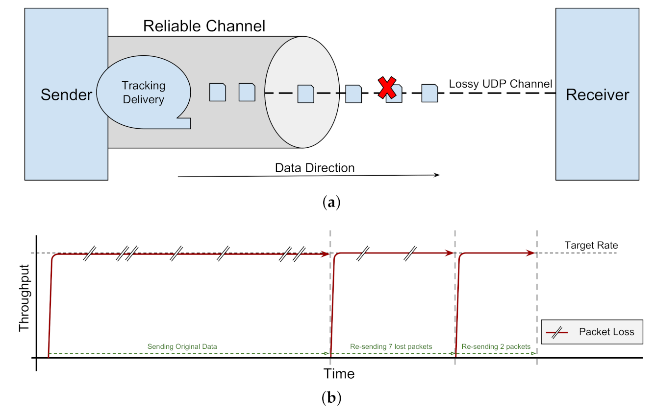
Figure 4.
Testbed Network Architecture. (a) Physical Network Configuration. (b) Overlay-1: Logical Dumbbell Network (BW = 1 Gb/s, BtlBW = 500 Mb/s). (c) Overlay-2: Logical Dumbbell Network (BW = 10 Gb/s, BtlBW = 1 Gb/s).
Figure 4.
Testbed Network Architecture. (a) Physical Network Configuration. (b) Overlay-1: Logical Dumbbell Network (BW = 1 Gb/s, BtlBW = 500 Mb/s). (c) Overlay-2: Logical Dumbbell Network (BW = 10 Gb/s, BtlBW = 1 Gb/s).

Figure 5.
Testbed Hardware Configuration. (a) Parameter space. (b) Overlay-1: Nodes Configuration. (c) Overlay-2: Nodes Configuration.
Figure 5.
Testbed Hardware Configuration. (a) Parameter space. (b) Overlay-1: Nodes Configuration. (c) Overlay-2: Nodes Configuration.
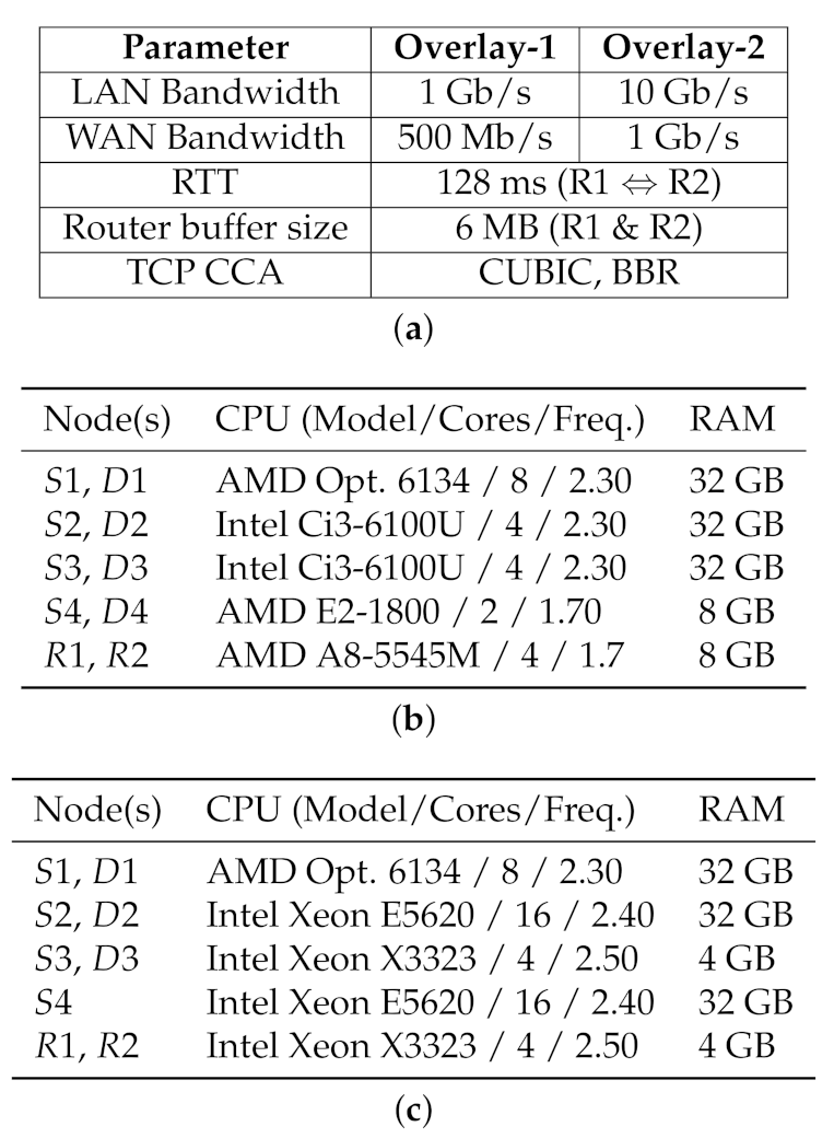
Figure 6.
Emulated network configuration commands for (a) end-nodes. (b) virtual router nodes.
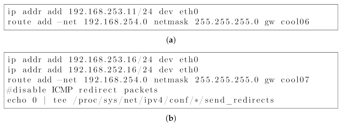
Figure 7.
Characterization of Synthetic Background Traffic. (a) Generated traffic pattern. (b) Configuration settings for generated traffic.
Figure 7.
Characterization of Synthetic Background Traffic. (a) Generated traffic pattern. (b) Configuration settings for generated traffic.
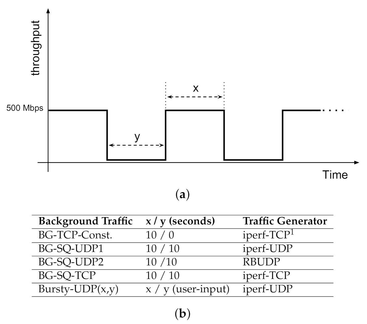
Figure 8.
Illustrative examples: active vs. passive probing impact on RTT signal: 90 s time-series signatures per traffic mixture. Active probing changes time-series patterns. Note the different ranges for Y-axis across columns.
Figure 8.
Illustrative examples: active vs. passive probing impact on RTT signal: 90 s time-series signatures per traffic mixture. Active probing changes time-series patterns. Note the different ranges for Y-axis across columns.

Figure 9.
Passive and Active Probing: RTT measurement (ping) combined with probing profile pattern based on bandwidth interference (iperf).
Figure 9.
Passive and Active Probing: RTT measurement (ping) combined with probing profile pattern based on bandwidth interference (iperf).

Figure 10.
The scope of our machine-learning study is TCP schemes, CUBIC and BBR in particular. (a) Interaction of CUBIC and BBR on a shared network. (b) Background Traffic Classes to be train a model.
Figure 10.
The scope of our machine-learning study is TCP schemes, CUBIC and BBR in particular. (a) Interaction of CUBIC and BBR on a shared network. (b) Background Traffic Classes to be train a model.

Figure 11.
Classification Models for Background Traffic Classification. (a) Inference Workflow. (b) Network Structure for MLP neural network.
Figure 11.
Classification Models for Background Traffic Classification. (a) Inference Workflow. (b) Network Structure for MLP neural network.

Figure 12.
Binary decision model for choosing a CCA for new data transfer.
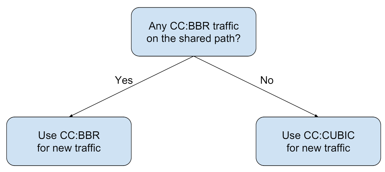
Figure 13.
(Overlay-1) Effect of TCP and UDP traffic competing for bandwidth (BW = 1 Gb/s, BtlBW = 500 Mb/s, RTT = 128 ms). (a) Scenario One: Effect of Square Pattern Background Traffic. (b) Scenario Two: Effect of Bursty UDP Background Traffic.
Figure 13.
(Overlay-1) Effect of TCP and UDP traffic competing for bandwidth (BW = 1 Gb/s, BtlBW = 500 Mb/s, RTT = 128 ms). (a) Scenario One: Effect of Square Pattern Background Traffic. (b) Scenario Two: Effect of Bursty UDP Background Traffic.

Figure 14.
(Overlay-2) Effect of TCP and UDP traffic competing for bandwidth (BW = 10 Gb/s, BtlBW = 1 Gb/s, RTT = 128 ms). (a) Scenario One: Effect of Square Pattern Background Traffic. (b) Scenario Two: Effect of Bursty UDP Background Traffic.
Figure 14.
(Overlay-2) Effect of TCP and UDP traffic competing for bandwidth (BW = 10 Gb/s, BtlBW = 1 Gb/s, RTT = 128 ms). (a) Scenario One: Effect of Square Pattern Background Traffic. (b) Scenario Two: Effect of Bursty UDP Background Traffic.

Figure 15.
(Scenario Three) Effect of NFS background traffic on throughput (Overlay-1 Network).

Figure 16.
Scenario Two: NFS mount-point over network.
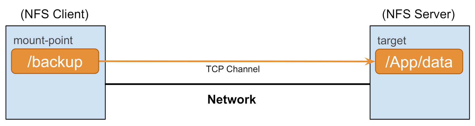
Figure 17.
(Overlay-1) Effect of different TCP CCAs competing for bandwidth: CUBIC vs. BBR (BW = 1 Gb/s, BtlBW = 500 Mb/s, RTT = 128 ms). (a) Background traffic: Constant TCP. (b) Background traffic : Square-wave TCP.
Figure 17.
(Overlay-1) Effect of different TCP CCAs competing for bandwidth: CUBIC vs. BBR (BW = 1 Gb/s, BtlBW = 500 Mb/s, RTT = 128 ms). (a) Background traffic: Constant TCP. (b) Background traffic : Square-wave TCP.

Figure 18.
(Overlay-2) Effect of different TCP CCAs competing for bandwidth: CUBIC vs. BBR (BW = 10 Gb/s, BtlBW = 1 Gb/s, RTT = 128 ms). (a) Background traffic: Constant TCP. (b) Background traffic: Square-wave TCP.
Figure 18.
(Overlay-2) Effect of different TCP CCAs competing for bandwidth: CUBIC vs. BBR (BW = 10 Gb/s, BtlBW = 1 Gb/s, RTT = 128 ms). (a) Background traffic: Constant TCP. (b) Background traffic: Square-wave TCP.
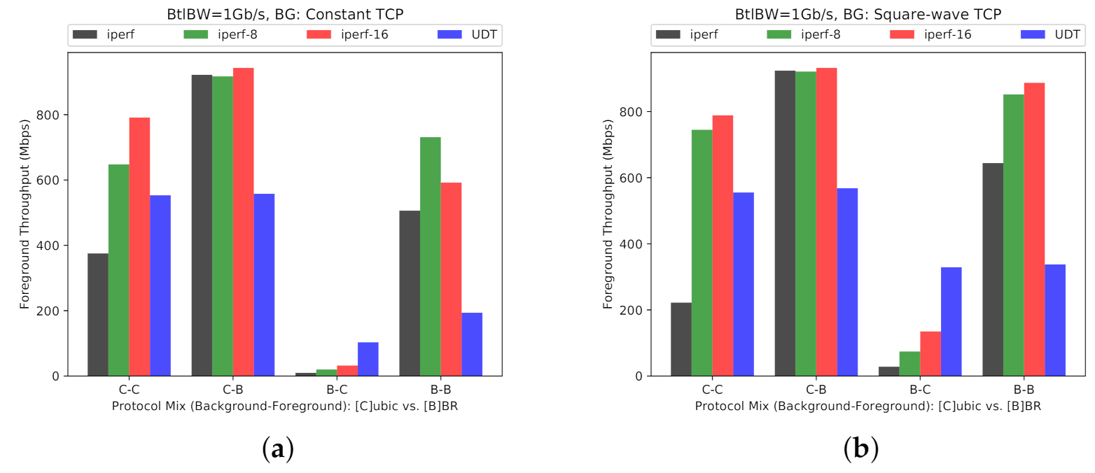
Figure 19.
Impact on NFS: Throughput of NFS-over-TCP with TCP and UDP background traffic (Overlay-1 Network). (a) Average NFS Throughput, Per Node-Pair. (b) Aggregate NFS Throughput, Per Node-Pair.
Figure 19.
Impact on NFS: Throughput of NFS-over-TCP with TCP and UDP background traffic (Overlay-1 Network). (a) Average NFS Throughput, Per Node-Pair. (b) Aggregate NFS Throughput, Per Node-Pair.

Figure 20.
RTT Variation (via ping) over Time, Due to Congestion.
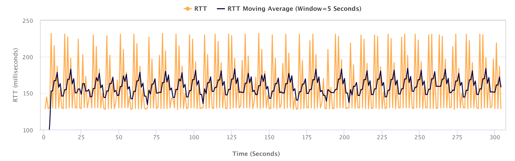
Figure 21.
Throughput of a standard CUBIC TCP stream in the presence of various background traffic for (a) Overlay-1 Network. (b) Overlay-2 Network.
Figure 21.
Throughput of a standard CUBIC TCP stream in the presence of various background traffic for (a) Overlay-1 Network. (b) Overlay-2 Network.

Figure 22.
(Passive Probing) Performance of classification models for varying time length w of the input time-series (5-Fold Cross-Validation). (a) Classification accuracy. (b) Box Plot for classifiers accuracy.
Figure 22.
(Passive Probing) Performance of classification models for varying time length w of the input time-series (5-Fold Cross-Validation). (a) Classification accuracy. (b) Box Plot for classifiers accuracy.

Figure 23.
(Passive Probing) K-NN (DTW) Performance (, ) (5-Fold Cross-Validation). (a) Confusion Matrix. (b) Classification Report on Accuracy-related metrics.
Figure 23.
(Passive Probing) K-NN (DTW) Performance (, ) (5-Fold Cross-Validation). (a) Confusion Matrix. (b) Classification Report on Accuracy-related metrics.

Figure 24.
(Active Probing) Accuracy of classification models for window size w of the input time-series with Active Probing (5-Fold Cross-Validation). 1-NN-MLN18 represents Passive Probing performance as the baseline [11]. (a) Classification Accuracy per window size. (b) Box Plot for Classifiers Accuracy.

Figure 25.
Accuracy variation (BoxPlot) of classification models for varying time length w of the input time-series per k in K-NN with DTW—with and without Active Probing (5-Fold Cross-Validation). (a) 1-NN w/ DTW with Active Probing. (b) 3-NN w/ DTW with Active Probing. (c) 5-NN w/ DTW with Active Probing. (d) 1-NN w/ DTW with Passive Probing.
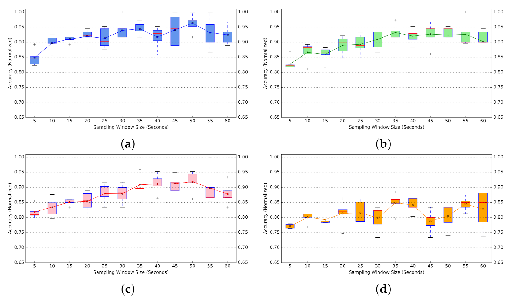
Figure 26.
Confusion Matrix for classification models for of the input time-series per k in K-NN with DTW, with and without Active Probing (5-Fold Cross-Validation). (a) 1-NN w/ DTW with Active Probing. (b) 3-NN w/ DTW with Active Probing. (c) 5-NN w/ DTW with Active Probing. (d) 1-NN w/ DTW with Passive Probing.

Figure 27.
K-NN (DTW) Performance (, ) with Active Probing. (a) Confusion Matrix. (b) Classification Metrics.
Figure 27.
K-NN (DTW) Performance (, ) with Active Probing. (a) Confusion Matrix. (b) Classification Metrics.

Figure 28.
K-NN (DTW) Performance (, ) with Passive Probing. (a) Confusion Matrix. (b) Classification Metrics.
Figure 28.
K-NN (DTW) Performance (, ) with Passive Probing. (a) Confusion Matrix. (b) Classification Metrics.

Figure 29.
Average throughput of fixed versus adaptive (OPS) data-transfer schemes. OPS improves throughput and fairness for foreground traffic by using a decision model. (a) Background Traffic=CUBIC, OPS improves fairness while maintaining a reasonable bandwidth by using CUBIC in foreground. (b) Background Traffic=BBR, OPS maintains fair throughput by using BBR in foreground.
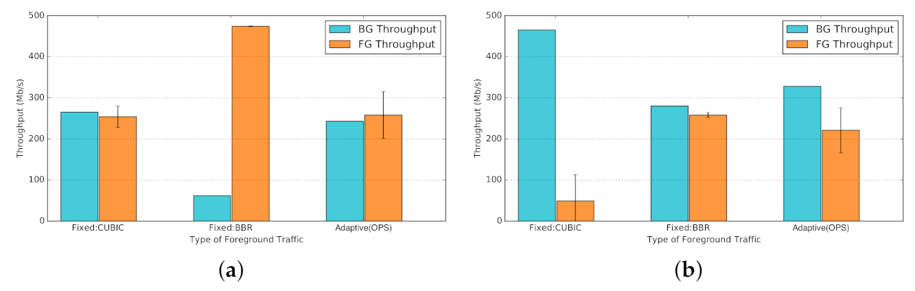

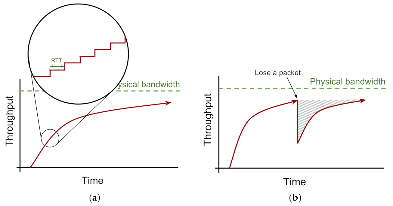
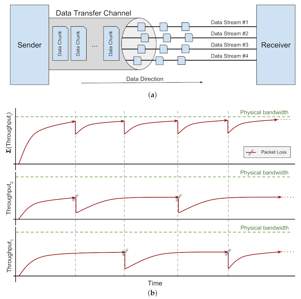
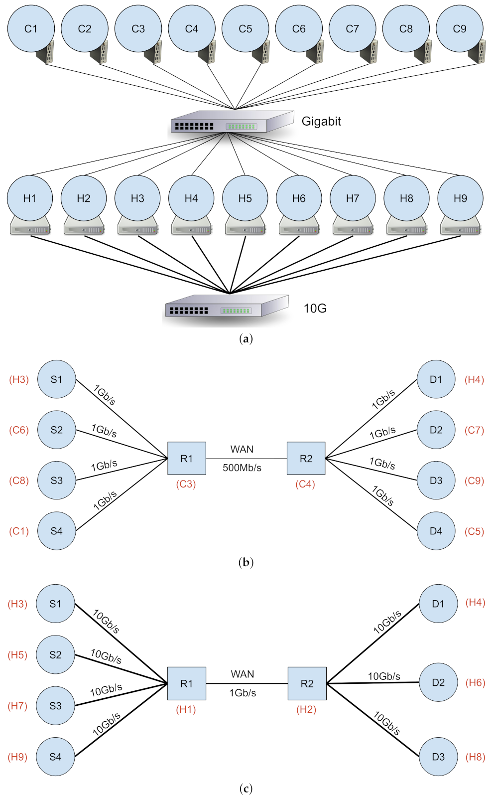
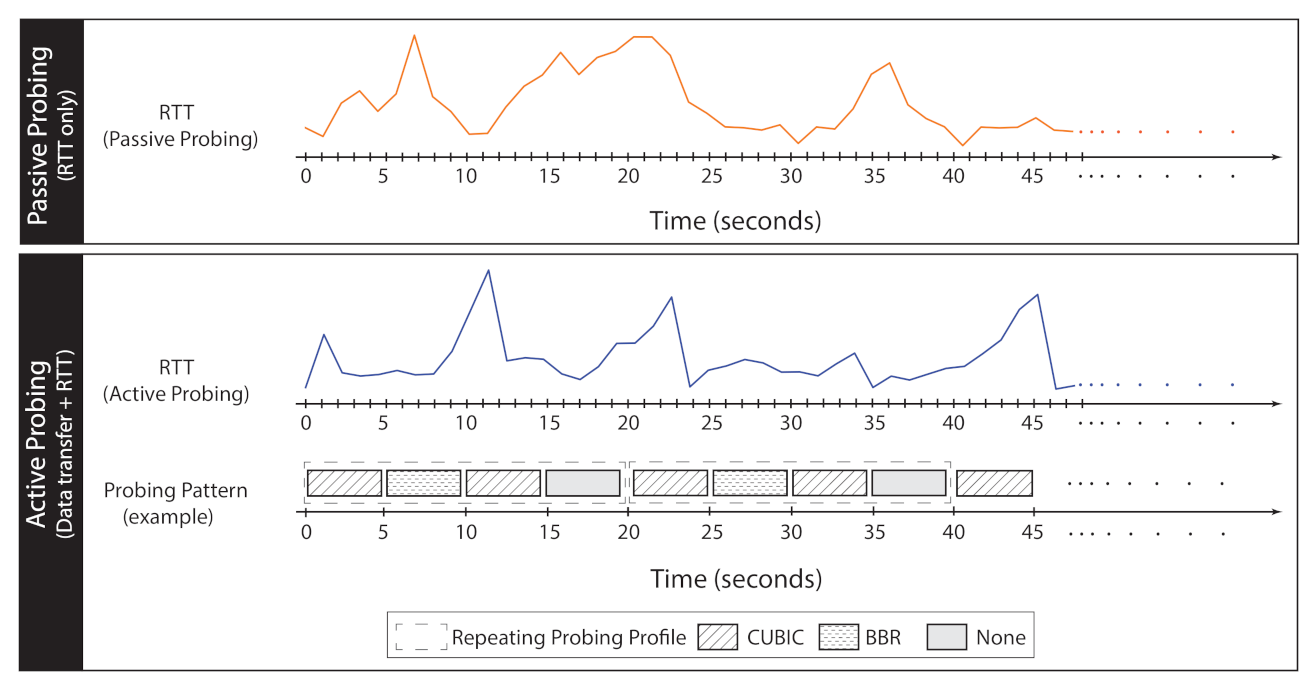
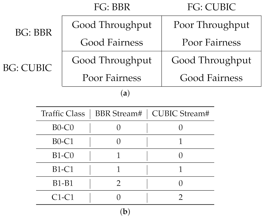
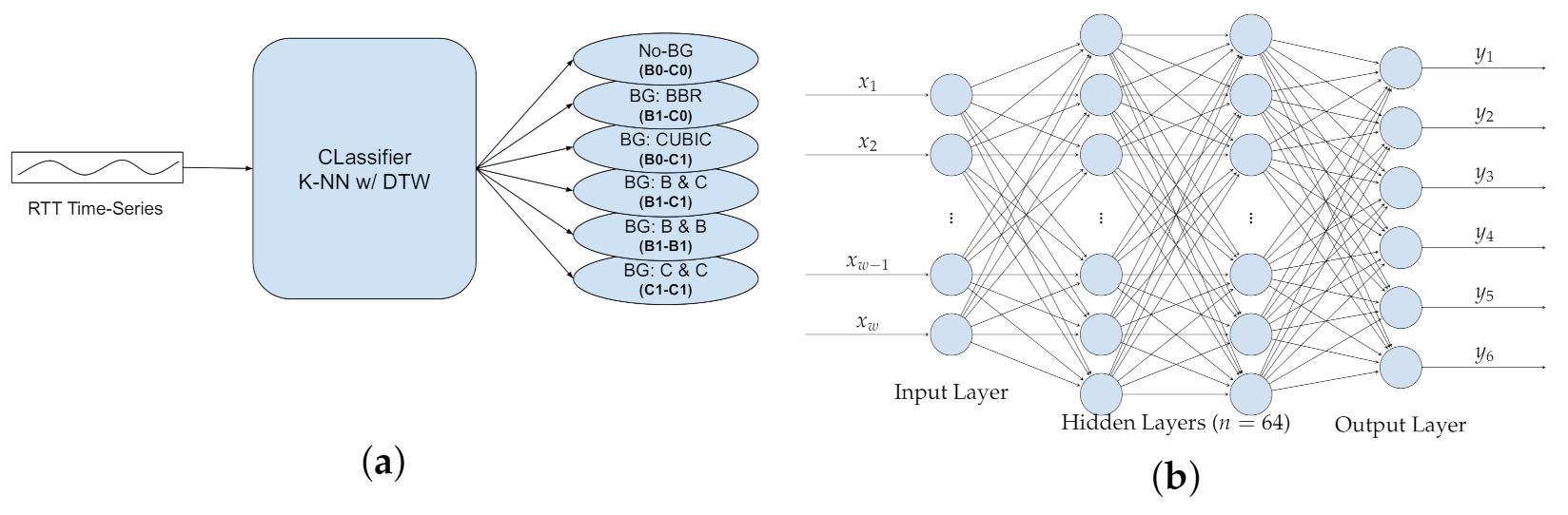
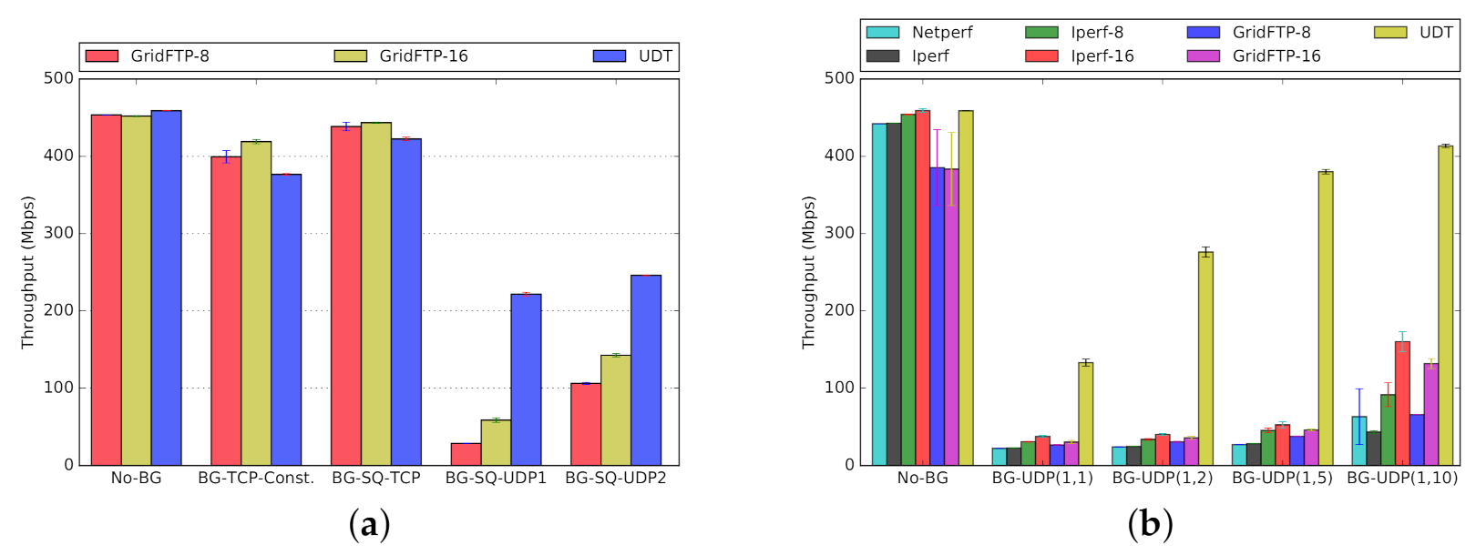
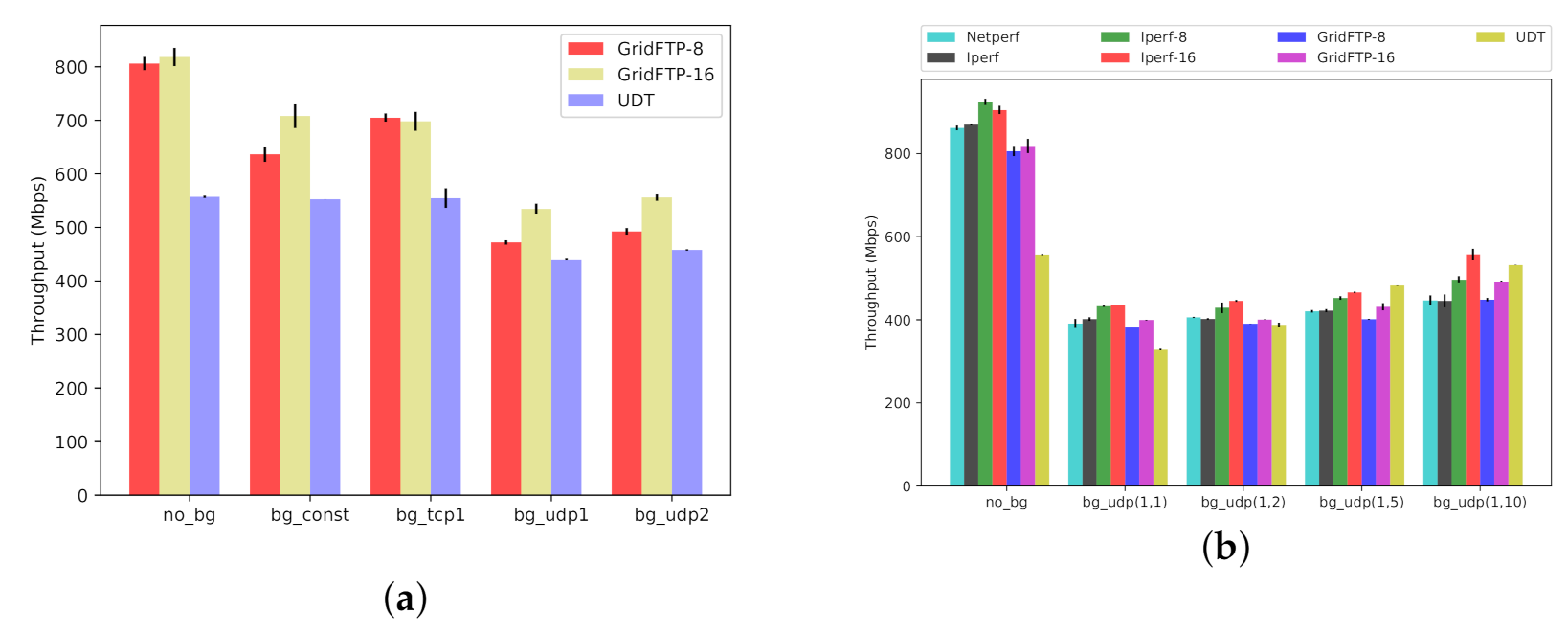
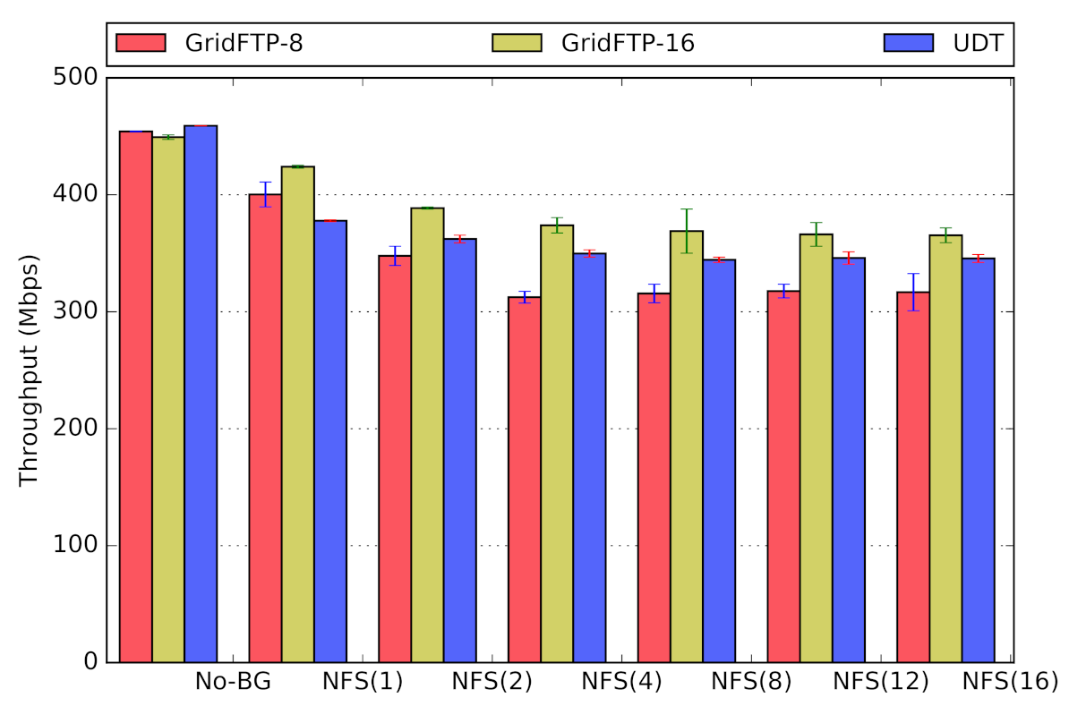
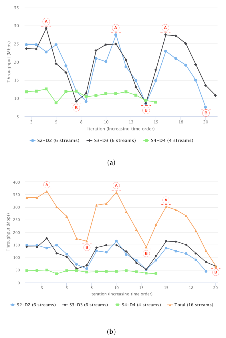
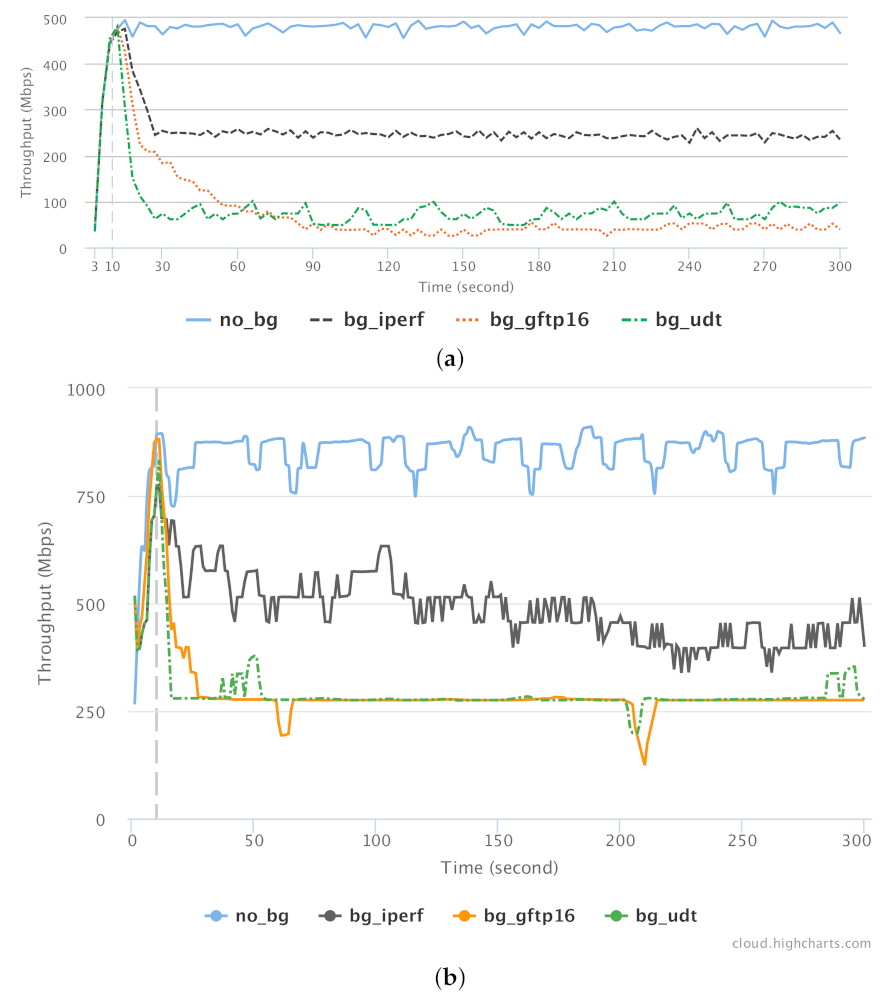
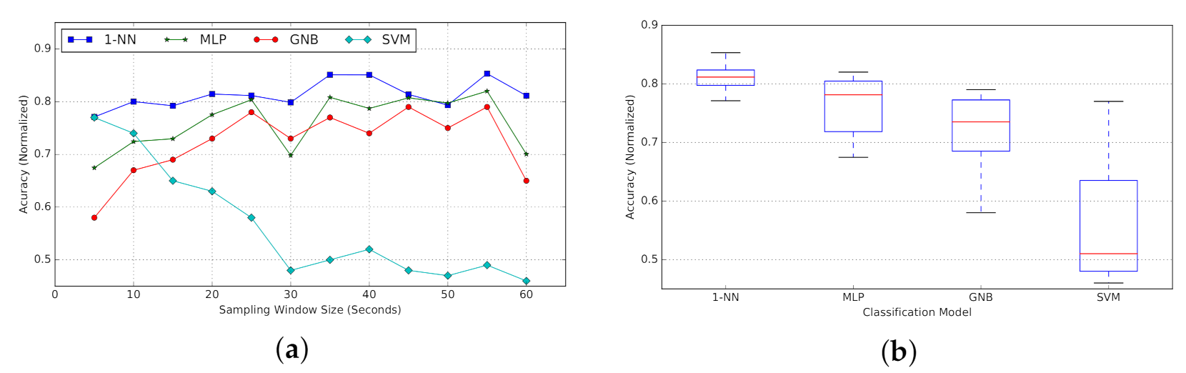
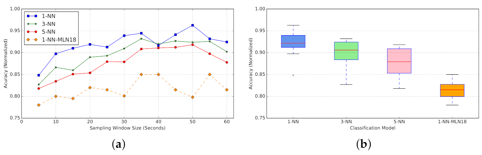
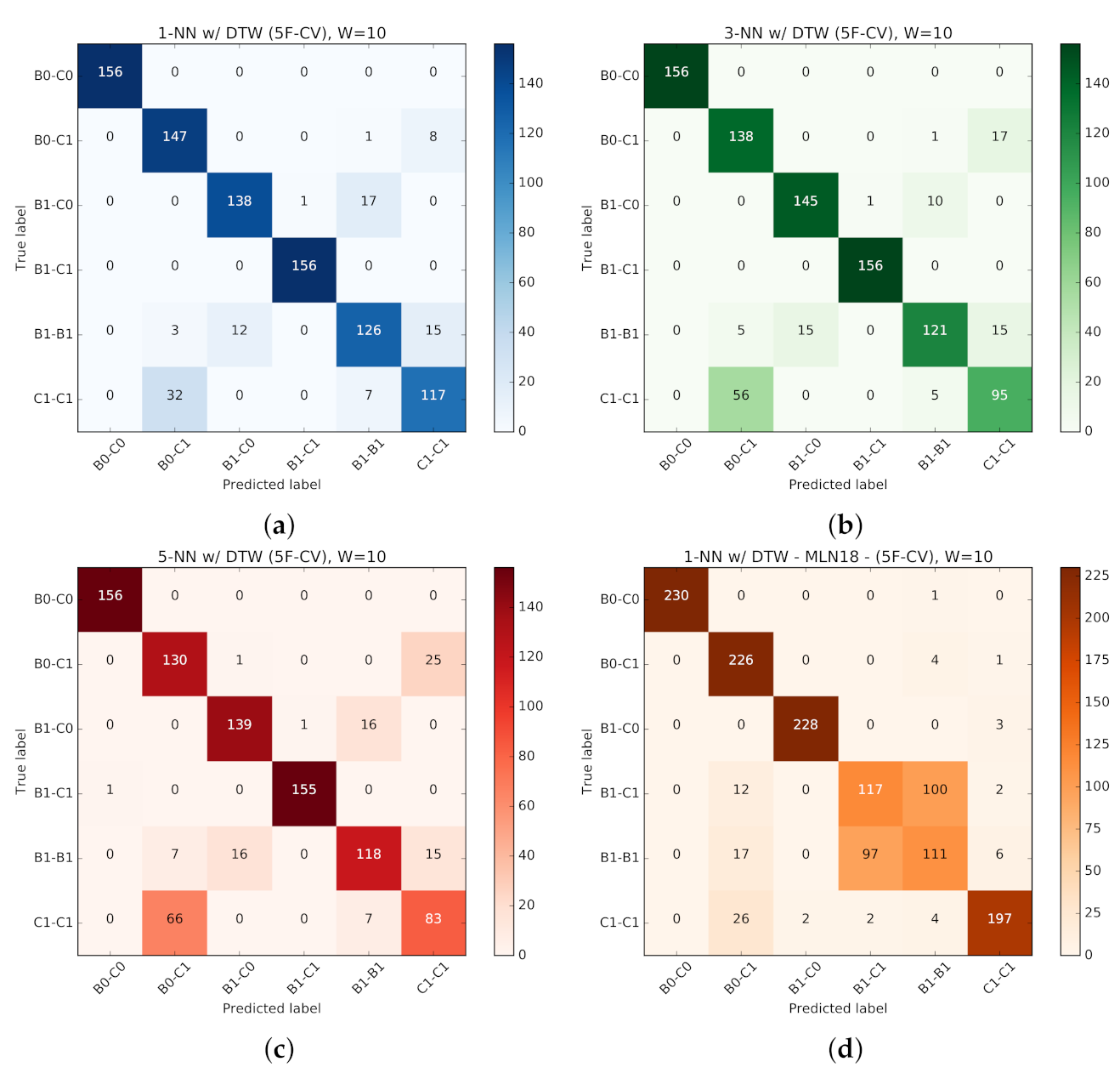
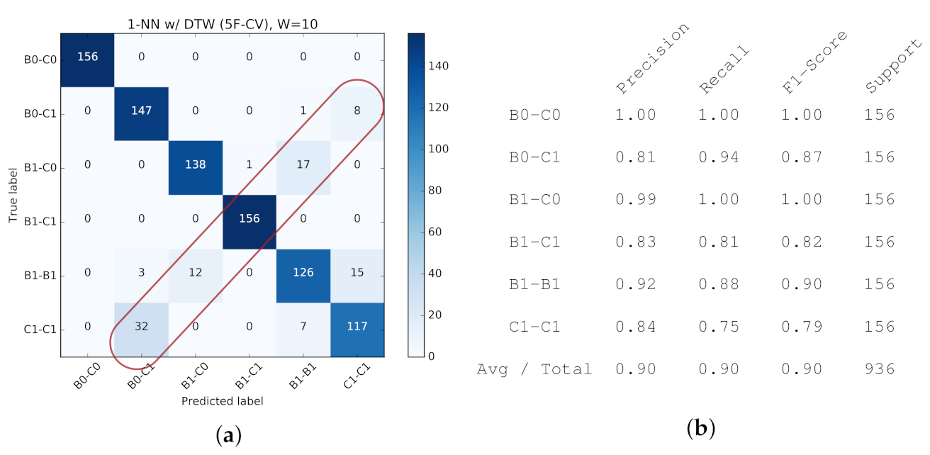
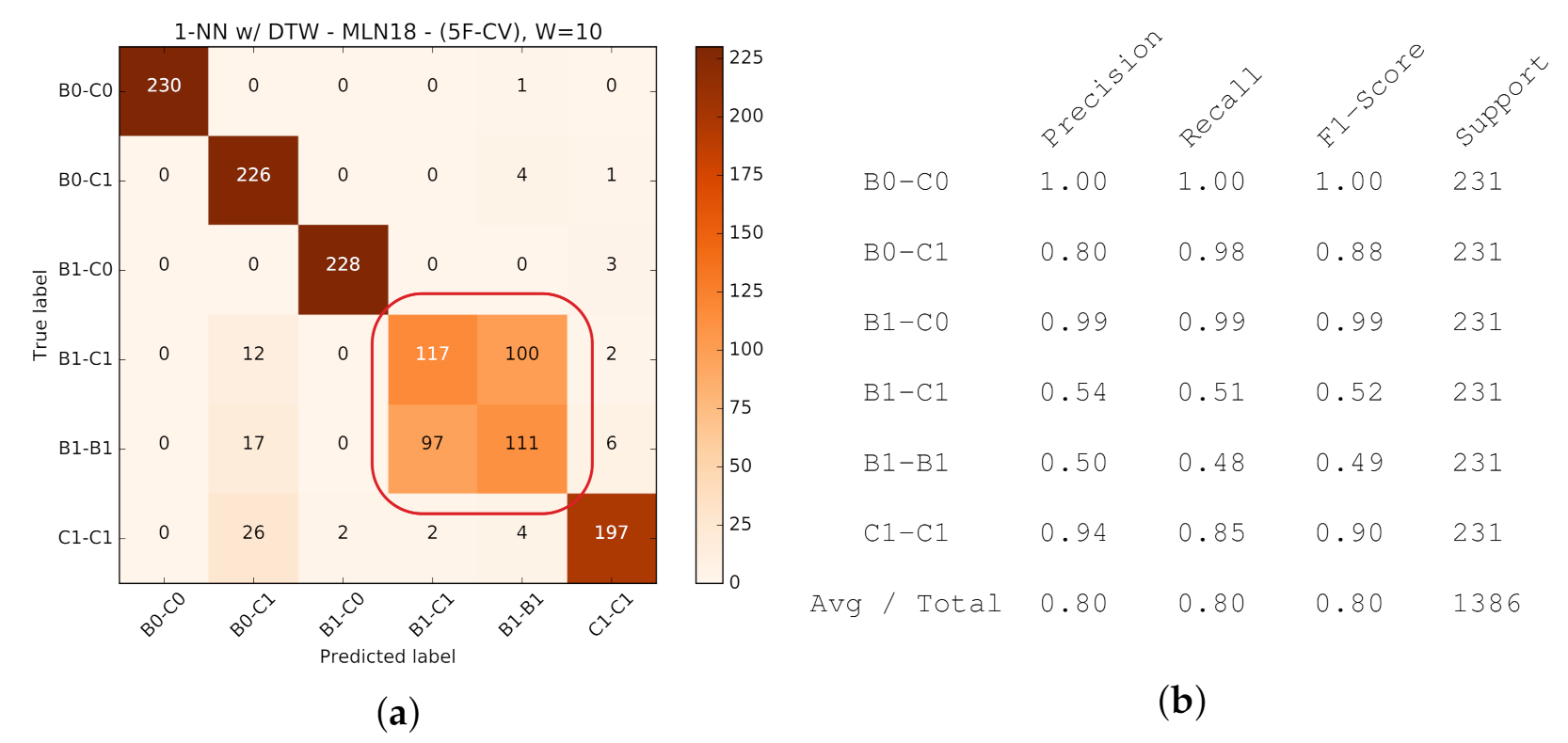
Table 1.
A summary of experimental results provided (Synthetic traffic: Figure 7, NFS: Figure 16).
Table 1.
A summary of experimental results provided (Synthetic traffic: Figure 7, NFS: Figure 16).
| Figure | Network | Traffic Mixture | Background | Note(s) |
|---|---|---|---|---|
| Figure 13 | Overlay-1 | TCP vs. UDP | Synthetic | Compare Figure 14 |
| Figure 14 | Overlay-2 | TCP vs. UDP | Synthetic | Compare Figure 13 |
| Figure 17 | Overlay-1 | CUBIC vs. BBR | Synthetic | Compare Figure 18 |
| Figure 18 | Overlay-2 | CUBIC vs. BBR | Synthetic | Compare Figure 17 |
| Figure 15 | Overlay-1 | TCP vs. UDP | Synthetic, NFS | No Overlay-2 results given |
| Figure 19 | Overlay-1 | TCP vs. UDP | Synthetic, NFS | No Overlay-2 results given |
| Figure 21a | Overlay-1 | TCP vs. UDP | Synthetic | Compare Figure 21b |
| Figure 21b | Overlay-2 | TCP vs. UDP | Synthetic | Compare Figure 21a |
Table 2.
Throughput (Mbps) and Jain fairness (0∼1) of well-known protocols on Overlay-1 Network. As evident by calculated Jain indices, GridFTP and UDT are considerably unfair to single TCP streams, GridFTP representing the lowest fairness index.
Table 2.
Throughput (Mbps) and Jain fairness (0∼1) of well-known protocols on Overlay-1 Network. As evident by calculated Jain indices, GridFTP and UDT are considerably unfair to single TCP streams, GridFTP representing the lowest fairness index.
| Type | Stream | no_bg | bg_iperf | bg_gftp16 | bg_udt |
|---|---|---|---|---|---|
| Dedicated | Background | - | 478 | 473 | 481 |
| Foreground (iperf) | 474 | 474 | 474 | 474 | |
| Shared | Background | - | 238 | 415 | 398 |
| Foreground (iperf) | 474 | 253 | 75.6 | 85.3 | |
| Jain fairness | - | 1 | 0.68 | 0.7 |
Table 3.
Throughput (Mbps) and Jain fairness (0∼1) of well-known protocols on Overlay-2 Network. As evident by calculated Jain indices, the fairness issues with GridFTP and UDT are consistently manifested regardless of the varying BDP (bottleneck-bandwidth and RTT).
Table 3.
Throughput (Mbps) and Jain fairness (0∼1) of well-known protocols on Overlay-2 Network. As evident by calculated Jain indices, the fairness issues with GridFTP and UDT are consistently manifested regardless of the varying BDP (bottleneck-bandwidth and RTT).
| Type | Stream | no_bg | bg_iperf | bg_gftp16 | bg_udt |
|---|---|---|---|---|---|
| Dedicated | Background | - | 848 | 811 | 625 |
| Foreground (iperf) | 872 | 872 | 872 | 872 | |
| Shared | Background | - | 412 | 738 | 591 |
| Foreground (iperf) | 872 | 485 | 109 | 161 | |
| Jain fairness | - | 0.99 | 0.64 | 0.75 |
Publisher’s Note: MDPI stays neutral with regard to jurisdictional claims in published maps and institutional affiliations. |
© 2021 by the authors. Licensee MDPI, Basel, Switzerland. This article is an open access article distributed under the terms and conditions of the Creative Commons Attribution (CC BY) license (https://creativecommons.org/licenses/by/4.0/).
Share and Cite
MDPI and ACS Style
Anvari, H.; Lu, P. Machine-Learned Recognition of Network Traffic for Optimization through Protocol Selection. Computers 2021, 10, 76. https://0-doi-org.brum.beds.ac.uk/10.3390/computers10060076
AMA Style
Anvari H, Lu P. Machine-Learned Recognition of Network Traffic for Optimization through Protocol Selection. Computers. 2021; 10(6):76. https://0-doi-org.brum.beds.ac.uk/10.3390/computers10060076
Chicago/Turabian StyleAnvari, Hamidreza, and Paul Lu. 2021. "Machine-Learned Recognition of Network Traffic for Optimization through Protocol Selection" Computers 10, no. 6: 76. https://0-doi-org.brum.beds.ac.uk/10.3390/computers10060076
Note that from the first issue of 2016, this journal uses article numbers instead of page numbers. See further details here.