
Online Multimodal Inference of Mental Workload for Cognitive Human Machine Systems


1
School of Engineering, RMIT University, Bundoora, VIC 3038, Australia
2
THALES Australia—Airspace Mobility Solutions, WTC North Wharf, Melbourne, VIC 3000, Australia
3
Northrop Grumman Corporation, 1550 W. Nursery Rd, Linthicum Heights, MD 21090, USA
*
Author to whom correspondence should be addressed.
†
Distribution Statement A: Approved for Public Release; Distribution is Unlimited; #21-0655; Dated 26 April 2021.
Computers 2021, 10(6), 81; https://0-doi-org.brum.beds.ac.uk/10.3390/computers10060081
Submission received: 19 April 2021
/
Revised: 9 June 2021
/
Accepted: 11 June 2021
/
Published: 16 June 2021
(This article belongs to the Special Issue Machine Learning for EEG Signal Processing)
Abstract
:With increasingly higher levels of automation in aerospace decision support systems, it is imperative that the human operator maintains the required level of situational awareness in different operational conditions and a central role in the decision-making process. While current aerospace systems and interfaces are limited in their adaptability, a Cognitive Human Machine System (CHMS) aims to perform dynamic, real-time system adaptation by estimating the cognitive states of the human operator. Nevertheless, to reliably drive system adaptation of current and emerging aerospace systems, there is a need to accurately and repeatably estimate cognitive states, particularly for Mental Workload (MWL), in real-time. As part of this study, two sessions were performed during a Multi-Attribute Task Battery (MATB) scenario, including a session for offline calibration and validation and a session for online validation of eleven multimodal inference models of MWL. The multimodal inference model implemented included an Adaptive Neuro Fuzzy Inference System (ANFIS), which was used in different configurations to fuse data from an Electroencephalogram (EEG) model’s output, four eye activity features and a control input feature. The online validation of the ANFIS models produced good results, while the best performing model (containing all four eye activity features and the control input feature) showed an average Mean Absolute Error (MAE) = 0.67 ± 0.18 and Correlation Coefficient (CC) = 0.71 ± 0.15. The remaining six ANFIS models included data from the EEG model’s output, which had an offset discrepancy. This resulted in an equivalent offset for the online multimodal fusion. Nonetheless, the efficacy of these ANFIS models could be confirmed by the pairwise correlation with the task level, where one model demonstrated a CC = 0.77 ± 0.06, which was the highest among all of the ANFIS models tested. Hence, this study demonstrates the suitability for online multimodal fusion of features extracted from EEG signals, eye activity and control inputs to produce an accurate and repeatable inference of MWL.
1. Introduction
1.1. Background
Dynamic, complex systems in modern aerospace operations become problematic when looking at the human’s response to automation. A number of complex tasks are not achievable without assistance from the system automation. Nonetheless, it is noted in the literature that automation has its consequences [1,2,3], as some of the main contributors to aviation accidents are attributed to human errors as a result of automation bias, complacency [4] and deterioration of manual flying skills [5]. With these concerns regarding the integration of automation in aerospace operations, there is a need for a new method of interaction between human operators and machines. This form of interaction moves away from architectures that treat automation and human activities as independent, toward Cyber–Physical System (CPS) architectures that support the development of a new generation of adaptive and cognitive Human–Machine Systems (HMS), collectively named Cyber–Physical–Human Systems (CPHS). These human-centric systems facilitate the cooperation of humans with machines, and are designed so that the skills and abilities of humans are not replaced; rather, they co-exist with and assist humans in performing more efficiently and effectively [6]. A Cognitive Human Machine System (CHMS) addresses this with a cyber–physical, human-centered design that provides necessary, real-time system adaptation [7,8]. A CHMS provides real-time system adaptation by collecting physiological and behavioral as well as mission, environmental and operational data (i.e., performance measures), which are fused in real-time to provide a final estimation of the operator’s cognitive states, such as Mental Workload (MWL), mental fatigue and attention. Among the cognitive states, MWL is of particular importance, as it directly affects the system performance [9]. MWL is a complex construct and is challenging to define accurately [10]. However, a general definition of MWL is defined as “the relation between the function relating the mental resources demanded by a task and those resources available to be supplied by the human operator” [11].
1.2. Physiological and Behavioral Responses
To reliably drive system adaptation (within an operational CHMS), there is a need to provide accurate and repeatable estimations of cognitive states in real time by further developing suitable models and algorithms that can infer MWL based on multiple real-time, physiological, behavioral and performance measurements. Such measurements have been extensively researched for detecting physiological and behavioral responses associated with MWL, including the use of sensors, such as Electroencephalogram (EEG) [12], Functional Near Infrared Spectroscopy (fNIR) [13], eye activity tracking [14], Electrocardiogram (ECG) [15], Galvanic Skin Response (GSR) [16] and control inputs [17]. Corresponding features associated with MWL include, among others: changes in theta (θ, 4–7 Hz) and alpha (α, 8–12 Hz) power bands with the EEG [12,18,19]; changes in Blinks Per Minute (BPM) [20,21], proportion dwell time [14], pupil diameter [22,23] and scan pattern behavior [24] with eye activity measures; changes in Heart Rate (HR) and Heart Rate Variability (HRV) [15,25] as well as respiration [26] with cardiorespiratory sensors; and, lastly, changes in accuracy and response time as well as mouse movements with a computer mouse used for control inputs [17].
The EEG has shown to be beneficial for the measurement of MWL; however, EEG signals are particularly prone to internal and external artifacts as well as volume conduction, which can blur the signal on the surface of the scalp [27,28]. As such, with the use of an EEG, it is vital to implement methods such as spatial filtering that can select appropriate features. Spatial filtering can do this by obtaining a smaller number of new channels that are based on a linear combination of the original channels [29]. This significantly reduces the dimensionality of the EEG features and more accurately locates where the signals originate. The use of adaptive spatial filters includes implementing data-driven spatial filters that are optimized with supervised learning for each subject. A commonly used adaptive spatial filter is the Common Spatial Patterns (CSP) [30,31]. However, more recently, the Source Power Comodulation (SPoC) was developed. The SPoC is an adaptive spatial filter similar to CSP but tailored for continuous estimations, as it extracts an oscillatory source that shows a comodulation with the power and a given target variable [31,32]. An expansion of such filters includes selecting several desired frequency bands and then producing a pre-determined number of spatial filters for each band. One such method is described for Filter Bank CSP (FBCSP) by Ang et al. [33], but also applies for a Filter Bank SPoC (FBSPoC). This method ensures that the best spectral and spatial filters are obtained since each resulting feature associates to a specific frequency band and spatial filter. However, using this method can produce a relatively large number of features. Consequently, for continuously estimating MWL (given EEG features generated from FBSPoC), it is preferred to use a shrinkage method, given that many of the features are expected to not contain relevant information. One such shrinkage method is ridge regression, and is a method that shrinks the regression coefficients by imposing a penalty on their size [34]. This means that non-informative features are minimized in their contribution to the inference of MWL.
Although many of the aforementioned physiological and behavioral responses are sensitive to changes in MWL, two recent reviews have reported that the physiological and behavioral responses of MWL are not universally valid for all task scenarios [35,36]. Both reviews identified multiple studies that reported statistical significance in physiological and behavioral measures that can measure MWL for different task scenarios. However, the reviews noted that the measures were sensitive depending on the task type and difficulty. Therefore, there was not identified a measure of MWL that could be generalized across various tasks.
Previous studies have implemented various task loads for provoking MWL, using many different task scenarios, including the following: simpler task scenarios in controlled laboratory environments, such as n-back task, arithmetic task, Hampshire tree task, Sternberg task and other equivalent tasks [37,38]; somewhat more complex task scenarios that require multi-tasking, such as Multi-Attribute Task Battery (MATB) [39] or the automated Cabin Air Management System (aCAMS) [40]; task scenarios that generate complex task loads, such as Air Traffic Management (ATM) simulations [18,19] or flight simulations [25,41]; and lastly, a limited number of studies have used real operational conditions, such as actual flight [42] or driving scenarios [43].
1.3. Multimodal Fusion for Inferring MWL
The process of estimating cognitive states (i.e., MWL) in a CHMS includes translating the respective features into a certain command. Studies have implemented the use of supervised Machine Learning (ML) techniques for estimating MWL during a specific task scenario by either implementing classification algorithms for classifying MWL between discrete states, or the use of regression algorithms for continuously inferring MWL. These ML techniques are used for fusing features within a single modality, generally using the EEG [38,44] or fNIR [41], but are also used for fusing features across modalities [45,46].
Among the ML techniques, classification algorithms are most commonly used [29]. Classification algorithms include classifying between discrete MWL states (i.e., resting, low and high) with the use of ML models, such as Artificial Neural Networks (ANN) [47,48], Support Vector Machines (SVM) [38,49] or Linear Discriminant Analysis (LDA) [19,41] (or extended variants). In addition to this, some studies compare several classification models when performing MWL estimations [50,51]. The use of regression models, such as Neuro Fuzzy Systems (NFS) [46,52,53] and Gaussian process regression [44], provides a continuous estimation of MWL but is less reported. Many of the studies that perform multimodal data fusion implement ML techniques that perform the calibration and validation in offline processing. Nonetheless, real-time data processing often shows variable and inconsistent results.
Some studies performed online validation of multimodal data fusion models [45,48,54]. Notably, Wilson and Russell [48] conducted a study in which an ANN was used to fuse data from EEG features (band-power from delta, theta, alpha, beta and gamma from six electrodes), eye activity features (blinks and interblink intervals) and cardiorespiratory features (respiration, HR and HRV) in a MATB task scenario, using resting, low and high task-load conditions. Here, the ANN performed online classification on the respective task load at 5 s intervals and demonstrated a classification accuracy of 84.3%.
Other studies performed elements of real-time system adaptation by using measures of MWL. However, these studies generally used models that implement a single modality, such as EEG [19], fNIR [13] or task performance [55]. Ting et al. [53] conducted one of few studies performing real-time system adaptation by implementing a multimodal data fusion model. In this study, EEG features, HRV and a task performance measure were used to drive system adaptation in an aCAMS simulation. However, the physiological measures were sampled at long, 7.5 min intervals.
In terms of estimating MWL, a continuous regression measure of MWL is arguably more suited for driving system adaptation in a closed loop system, such as the CHMS. Among the regression type models, NFS are of particular interest, as they are suitable for fusing data from multiple modalities and are more transparent than other ML methods. Thus, it overcomes some of the “black box” problems that are faced by many of the other ML methods. NFS can optimize the parameters of a Fuzzy Inference System (FIS) based on calibration data, and one notable method includes the Adaptive Neuro Fuzzy Inference System (ANFIS) [56]. The ANFIS is a method that utilizes both the advantages of a FIS and neural networks. The ANFIS tunes the fuzzy sets and fuzzy rules based on a calibration phase that implements labeled data. To generate the fuzzy rules, the ANFIS implements a Takagi Sugeno type processing technique [46,56,57].
There are few studies employing NFS for MWL estimation. In studies by Zhang et al. and Ting et al. [53,58,59], a Genetic Algorithm (GA)-based Mamdani fuzzy model was used to optimize the FIS parameters. Here, 7.5 min intervals were used, with features from an EEG and cardiac sensor. An extension of this work was further presented in a study conducted by Wang et al. [46], with 2 min intervals, using Differential Evolution (DE) and Differential Evolution Algorithm with Ant Colony Search (DEACS) as means to optimize the ANFIS parameters. Zhang et al. and Wang et al. [46,58,59] demonstrated good results in an offline calibration and validation with the aforementioned models. Nevertheless, they also implemented a conventional ANFIS model for comparison, which showed poor results. Lim et al. [52] also implemented an ANFIS model in their study, which was calibrated on data from cardiac features, eye activity features and features from an fNIR. The offline validation showed good results from calibrating the model on the normalized features, but the study failed to demonstrate good results during the online validation.
Hence, these studies failed to implement a conventional ANFIS paradigm to produce accurate results of the online inference of MWL. Whereas studies by Zhang et al. and Wang et al. [46,58,59] demonstrated large time intervals, Lim et al. [52] lacked the ability to demonstrate an inference of MWL during an online validation. Moreover, recent studies have outlined the importance of investigating the features contributing to the performance of the respective model used [50,51]. This is also an area that was not investigated for NFS in previous studies. Lastly, cross-session models are other important considerations for inference models of MWL [60]. This includes calibrating a model in one session on one given day and validating the model on another day. This is vital for the operational effectiveness when implementing a CHMS.
1.4. CHMS Framework
The CHMS, initially described by Liu et al. [7], aims to provide real-time system adaptation that can dynamically change system functions and Human Machine Interface and Interaction (HMI2) formats. The configuration for the CHMS can be seen in Figure 1 and illustrates a closed-loop system. The CHMS consists of four fundamental components that include the human operator, sensing module, estimation module and adaptation module.
The CHMS is a system that consists of two heterogenous sensor networks, including physiological and behavioral sensors (detailed in Section 1.2), and other performance-based measures (e.g., deduced from primary and/or secondary mission objectives). These measures are fused in the estimation module to produce estimations of the human’s cognitive states that then drive the system adaptation. This then produces a new task load presented to the human operator, which results in new cognitive states of the human as well as new system conditions, and the cycle then repeats.
The integration of the CHMS can support aerospace systems to operate at higher levels of automation while ensuring that the human operator maintains a central role within the system and that trust in the system is maintained. Moreover, the CHMS can play an important role in the emergence of new operational aerospace systems, such as the transition from two pilots to Single Pilot Operation (SPO) in commercial aircrafts [7,61], One-To-Many (OTM) Unmanned Aerial Vehicle (UAV) operation [52,62], evolution of ATM [63] and Urban Traffic Management (UTM) [64].
1.5. Research Methodology and Objectives
While the CHMS includes driving real-time system adaptation, this study will focus on the multimodal sensing and estimation of MWL. The aim of this study is to develop an accurate and repeatable multimodal inference model for continuous, real-time inference of MWL as needed for a CHMS.
As part of this study, two different sessions were conducted where the participants performed a MATB task scenario that varied between low, medium and high task-load conditions, as well as pre- and post-resting phases. Session 1 included collecting physiological and behavioral data from an EEG, eye activity tracker, ECG and computer mouse. These data were then used for offline calibration and validation of several multimodal ANFIS models. Session 2 included participants performing two rounds of tasks (Round 1 and Round 2) and involved an online validation of several ANFIS models.
In both sessions the physiological and behavioral measures were analyzed for their sensitivity to changes in task load during a MATB scenario. This was conducted with the pairwise correlation between the respective features and the pre-determined task level. Moreover, as part of Session 1, the best performing features were used for offline calibration and validation of several multimodal ANFIS models. The performance of these models was analyzed by using different generic and subject specific feature combinations. Round 1 of Session 2 included assessing the online cross-session capability of several ANFIS models, which were tested for the participants that completed Session 1. Round 2 of Session 2 further analyzed the online inference of MWL from all applicable ANFIS models and all participants. In addition, Round 2 evaluated the online performance of the ANFIS models that were calibrated using a subject specific feature combination and was tested on the participants that completed Session 1. Lastly, this study analyzed the offline (Session 1) and online (Session 2) performance of an EEG model that implemented a FBSPoC and ridge regression model.
2. Materials and Methods
2.1. MATB Scenario
The MATB program, developed by NASA, was employed to controllably and repeatably provoke MWL [39]. This task scenario was chosen due to its validity and is representative of operational piloting tasks. The program is comprised of four main tasks, including a system monitoring task (SYSMON), a tracking task (TRACK), a communication task (COMM) and a resource management task (RESMAN).
To control the task load presented to the subjects, the task loads were divided into low, medium and high task levels. The low task level included performing two tasks simultaneously (TRACK and SYSMON), the medium task level included performing three tasks simultaneously (TRACK, SYSMON and COMM), while the high task level included performing all four tasks simultaneously.
2.1.1. Session 1 Scenario and Procedure
As illustrated in Figure 2, the task load for Session 1 consisted of an initial 3 min pre-resting period, followed by 34 min of performing the MATB tasks, again followed by a 3 min post-resting period. The MATB task load for Session 1 consisted of performing the low task level for 5 min, medium task level for 5 min and high task level for 7 min. This was repeated by the same incremental increase in task load for another 17 min.
2.1.2. Session 2 Scenario and Procedure
Session 2 included two different rounds where the session lasted approximately 1 h and 20 min for each subject, including sensor fitting and offline calibration in between the rounds. Round 1 included performing the low, medium and high task levels, which lasted for 4 min each. Round 2 consisted of the same pre-defined task levels but rearranged in another order with a different duration of length, as the task levels could last between 2 and 5 min. This was done to thoroughly test that the multimodal models were able to infer MWL. As such, the task scenario lasted for a total of 18 min and consisted of the task levels in the following order: low (2 min), high (5 min), medium (3 min), high (3 min), low (3 min) and medium (2 min). As in Session 1, both rounds in Session 2 included pre- and post-resting, lasting 2 min each. The task load profiles for both rounds in Session 2 are illustrated in Figure 2, with the x-axis indicating time in minutes.
2.2. Participants
The participants approached for these experiments included subjects that were within the working age population (18–67 years). For Session 1, 17 participants took part in the experiment. There were 10 females and 7 males that participated in the experiment and the average age was 29 with a standard deviation of ±8.2. For Session 2, 12 participants took part in the experiment. Among the participants from Session 1, six also took part in Session 2. Only six participated in the second session, due to the lack of necessary resources and the availability of the participants. In total, there were 5 females and 7 males that took part in Session 2, where the average age was 31 with a standard deviation of ±9.3. All research and data collection methods were approved by RMIT University’s College Human Ethics Advisory Network (CHEAN) (ref: ASEHAPP 72-16). All participants volunteered for the experiment and were not paid. Informed consent was given prior to the experiment.
2.3. Physiological and Behavioral Data Collection and Processing
2.3.1. EEG Data Collection and Processing
The actiCAP Xpress from BrainProducts GmbH was used for performing the EEG recordings. The layout of the cap follows the international 10–20 system, where 16 electrodes collect data at the locations F4, AFz, F3, FCz, C3, C4, CPz, T7, T8, P3, POz, P4, P7, P8, O1 and O2. When the participants were being fitted with the EEG, a minimum impedance below 5 kΩ was accepted. To achieve this, the unsatisfactory electrode was either jiggled or alcohol and/or gel was applied to the area.
To process the EEG data, the NeuroPype software (Intheon Labs, San Diego) was used, which allowed for advanced signal processing. The software is written in Python and is a commercial product but is free for academic purposes. The signal pipeline developed for performing the inference of MWL is illustrated in Figure 3 and allows for offline and online processing. The pipeline uses a variety of supervised ML models, including one for the adaptive spatial spectral filter, using the FBSPoC and a ridge regression model to make a final inference of MWL.
For the EEG pipeline, the data were first labeled by assigning data labels (based on the pre-determined task level) within 3 s epochs. All 16 data channels on the EEG actiCAP Xpress were selected for the experiment. Following this, a high-pass filter was applied to remove all frequencies below 4 Hz. Once all these steps were completed, the offline calibration of the adaptive spatial spectral filter could commence.
Calibrating the FBSPoC resulted in several spatial filters that gave a power time course that was calibrated to comodulate with the pre-defined task level. In this study, the theta (θ, 4–7 Hz), alpha (α, 8–12 Hz) and beta (β, 13–30 Hz) bands were selected as filter banks. For each filter bank, there were three pattern pairs selected, resulting in six filters for each band and a total of 18 filters. A following feature extraction was then performed that took the logarithm of the variance from the resulting output from the adaptive spatial spectral filters, which than gave 18 power time courses. These features were then used to calibrate a ridge regression model. As the number of features were relatively large, a shrinkage regression method (i.e., ridge regression) was used since some features were expected to not include relevant information. For the ridge regression model, a negative Mean Absolute Error (MAE) was used as the scoring metrics and the regularization parameters were set to 0.1, 0.5, 1, 5 and 10. The output from the ridge regression model was one inference of MWL, given the feature set. Lastly, the results from five-fold validation during offline calibration and the results from offline validation were saved to a Comma-Separated Values (CSV) file for each respective epoch. During real-time processing, the outputs were passed through to a JavaScript (JS) with Transmission Control Protocol/Internet Protocol (TCP/IP) as further elaborated in Section 2.4.1.
2.3.2. Eye Activity Features
The eye tracker used for this study was the Gazepoint GP3, which is a remotely desk-mounted device, that was positioned at the base of the monitor about 65 cm away from the subject. The sensor has a sampling rate of 60 Hz and measures various eye activity features with the use of an infrared camera and illuminator. The eye activity features extracted as part of this study included Scan Pattern Entropy (SPE), BPM, Pupil Diameter (DIA) and Proportional Dwell Time (DWELL).
The SPE is determined from gaze transitions between different Regions of Interest (ROI) and are generally represented in a matrix. The cells then represent the number (or probability) of transitions between two interfaces [24,52]. The SPE thus measures the randomness of the scanning patterns, and was given by the following:
where and were the rows and columns of the transition matrix respectively, was the probability of fixation of the present state (i.e., fixation at region given previous fixation at region ) and was the probability of fixation of the prior state (i.e., probability of the previous fixation). For this study, there were 42 ROI that were sectioned based on the MATB Human Machine Interface (HMI).
BPM was calculated based on the calculation from the Gazepoint GP3 and was the number of blinks in one minute calculated with a sliding window.
Pupil diameter was recorded with the Gazepoint GP3; the diameter for each pupil was taken at 15 samples a second. With each of the left and right pupil diameters, the average of the two was obtained to get one measure each second. After this, a moving average was applied by using a 15 s sliding window.
Dwell time is a measure of how long the participant’s gaze is within a given ROI. For the proportional dwell time measure, there were 4 ROI that were defined around the four main tasks of the MATB HMI. To calculate this measure, the dwell times for each individual ROI were first obtained. Then, they were summed and averaged, giving the total dwell time for all the regions. A moving average was then applied to highlight the predominant trends in the data, which was done with a 30 s sliding window.
2.3.3. Cardiac Feature
The ECG sensor used in this study was the Zephyr Bioharness 3, where the precision of the data is specified as 0 to 240 beats per minute (±1 beats per minute) and has a sampling rate of 250 Hz. With the raw cardiac signal, the HR was determined by the extrapolation of the time interval in seconds between two consecutive R waves (R-to-R) and was calculated by the Bioharness 3.
2.3.4. Control Input Feature
Along with the eye activity measures, the Control Inputs (CI) from the right mouse button clicks were recorded, using the Gazepoint GP3 hardware. The number of mouse button clicks was recorded for each second (with 15 samples a second) and a moving average using a sliding window of 30 s was then applied to highlight the trends of the CI feature.
2.4. Multimodal Inference Model
The multimodal inference of MWL was conducted by implementing an ANFIS, which used a Takagi Sugeno type processing technique to generate the fuzzy rules [46,56,57]. A few parameters needed to be manually defined, including the number of fuzzy sets, the type of membership function used, the number of calibration epochs and the type of pre-clustering method used.
The pre-processing for the offline calibration and validation data included ensuring that the vector length for each dataset was the same length, with a data point recorded at each second. This also included synchronizing the different sensor measurements by manually adjusting the time elapsed until the resting period started. The vector length of the EEG output was also resampled, as the recordings were conducted at three second intervals.
For this study, there were four fuzzy sets used. This was implemented as there were four separate states as defined by the task levels, consisting of resting, low level, medium level and high level. These states can also be interpreted as very low, low, medium and high MWL. For the fuzzy sets, the membership functions used as inputs and outputs to the ANFIS included a Gaussian membership function. Fuzzy C-Means (FCM) clustering was implemented for the pre-clustering, as it required less computational time and was less prone to overfitting the data.
The first phase of the calibration included performing the pre-clustering. After the initial clustering was completed, the second phase could commence, which included further tuning the parameters of the previously generated FIS. Backpropagation was used to tune the input membership functions and was iteratively tuned over 2000 epochs. The output membership functions were computed, using least squares estimation. This was not an iterative learning method and was only generated based on the current set of calibration data.
Once the calibration was completed, the FIS parameters were automatically tuned. To show the efficacy of the model’s performance, a certain part of the data was set aside for validating the model with unseen data. For Session 1, this included reserving the second half, while for Session 2, the FIS was exported and implemented in a JS script that allowed for online validation. The processing methodology is illustrated in Figure 4.
2.4.1. Networking during the Experiment
Different processing was performed during Session 1 and 2 of this study. Whereas the calibration and validation for Session 1 was performed offline, Session 2 performed the calibration offline, while the validation of the models was performed online. For Session 1, the various eye activity features and HR feature were processed and received in real-time with a variety of JS scripts that then saved the features to a CSV file. In Session 1, the EEG data were recorded, using the BrainVision Recorder software, which saved the data to a vhdr file. Once all the data were collected, the offline calibration and validation of the ANFIS models were performed, using MATLAB scripts and the FIS toolbox. Round 1 of Session 2 was comprised of both collecting calibration data and performing cross-session validation for the applicable ANFIS models and subjects. Once Round 1 was completed, the within-session ANFIS models were calibrated, and the FIS files were exported for online processing in a JS script. The full network was implemented in Round 2 and included a server that received all the input features and forwarded it to the various ANFIS models that performed the inference of MWL in real-time.
2.5. Data Analysis
To assess the individual features, the pairwise Correlation Coefficient (CC) between the features and task level was implemented. For the inference models, the MAE was used to determine the error between the inference of MWL and the task level. Moreover, the CC was further used to analyze the efficacy of the inference models implemented. The respective analysis methods are given below.
2.5.1. Correlation Coefficient (CC)
To investigate the linear relationship between the various features and the pre-determined task level, the Pearson CC was calculated using Equation (2):
here, is the number of data points while is the feature and is the target value (e.g., task level). The target value and all the features were normalized between 0 and 1, prior to calculating the CC.
2.5.2. Mean Absolute Error (MAE)
The analysis from validating the inference models included performing an error calculation by using the MAE. The MAE is the average difference of the absolute value between the inference of MWL and the target value and was given by the following:
here, is the number of samples while is the target value (e.g., task level) and is the inferred value.
2.5.3. Testing for Normality
To validate the experimental results, a normality test was carried out on the outputs from the ANFIS models. The normality test was performed to ensure that no non-Gaussian disturbances were unintentionally introduced. The normality test was conducted, using the Kolmogorov–Smirnov test and was well suited, as it required ordinal data. To perform the Kolmogorov–Smirnov test, the “kstest” function in MATLAB was used with an alpha of 0.05. The normality test was performed on the ANFIS models’ offline output from Session 1 (ANFIS models 1 to 11), and the ANFIS models’ online output from Session 2. The results from performing the normality test demonstrated that the outputs from the ANFIS models passed the test. For the sake of conciseness, the detailed normality test results are not included.
2.5.4. Threshold Criterion
As part of the analysis, a threshold criterion was set for the ANFIS models’ online outputs (Session 2). This was conducted by obtaining the median of the respective dataset and determining upper and lower thresholds that were three scaled mean absolute deviations away from the median. Any sample that exceeded the thresholds were identified as an outlier and replaced with either the upper or the lower threshold value depending on which threshold was breached. MATLAB was used for identifying and replacing outliers for which the “isoutlier” function was implemented.
In Round 1, the threshold criterion applied to the online outputs from the ANFIS models 1 to 5. Overall, there were 812 outliers that were identified out of a total of 28,800 samples (960 × 5 × 6 = 28,800). For Round 2, the threshold criterion also applied to all online outputs from the ANFIS models. There were 7206 samples identified as outliers out of 173,240 samples (1320 × 11 × 12 = 173,240).
3. Results from Session 1
The results from Session 1 are presented in three different sections. The first section (Section 3.1) outlines the results from offline calibration and validation of the EEG model. Section 3.2 details the results from the pairwise correlation between all the features. Lastly, Section 3.3 details the results from the offline calibration and validation of the multimodal ANFIS models. The ANFIS models were tested with several different generic feature combinations as well as using a subject-specific feature combination.
3.1. Offline Validation of the EEG Model
The results from the offline calibration and validation of the EEG model are presented in Table 1 and is the average across all the subjects. Examining the five-fold validation results from calibrating on the first half of the data showed an average MAE of 0.47 with a standard deviation of ±0.09. Further examining the results from offline validation on the second half of the data showed an average MAE of 0.81 ± 0.38. This was a notable increase in the MAE with a larger standard deviation. The increase in standard deviation could be reflected in some of the cases where the MAE is high, e.g., for two participants that had a MAE of 2.1 and 1.20. This indicated that the EEG model performed poorly for these subjects. On the other hand, for several participants, the EEG model performed proficiently, where the lowest MAE was 0.50.
The efficacy of the EEG model’s ability to infer MWL could be seen with the offline validation conducted on unseen data. Nonetheless, the full vector length was needed for fusing the multimodal data with the ANFIS model. Thus, the results from the five-fold validation from calibrating the model on all the data showed a MAE of 0.60 ± 0.10.
3.2. Pairwise Correlation Analysis of the Individual Features
Before calibrating the ANFIS models, the individual features were analyzed by performing the pairwise correlation of each feature with the task level. As seen in Table 2, the strongest correlation across all participants was the pairwise correlation for the EEG, SPE and CI. Here the average across all participants was CC = 0.75, CC = 0.77 and CC = 0.82 respectively, with none of the subjects having a noticeable deviation from the average.
The results with moderate-level correlations across all participants was BPM, pupil diameter and proportional dwell time, which showed an average correlation of CC = −0.45, CC = 0.48 and CC = −0.55, respectively. For pupil diameter, most participants showed a positive correlation with the task level; however, two of the subjects showed a high negative correlation. Taking the absolute average of all these measures demonstrated that the average correlation was 0.60. For the features with moderate-level correlations, the standard deviation was relatively high. This indicated that for several participants, the feature was highly sensitive, while the other participants showed a low-level correlation. The results with an average low-level correlation included HR, with an average of CC = 0.31 ± 0.18.
3.3. Results from Offline Calibration and Validation of the ANFIS Models
This section details the results from offline calibration and validation of the ANFIS models. This included calibrating the ANFIS models with several feature combinations in order to analyze how each of the feature combinations performed. This section presents the results from calibrating the ANFIS on the second half of the data and validating the ANFIS on the first half of the data.
Figure 5 displays the results from calibrating and validating the ANFIS model on separate halves of the data. Upon examining the output from the ANFIS model (calibrated with all seven features), the inference of MWL closely matches the task level (see Figure 5). Nonetheless, there are some instances, particularly at the beginning of the low and medium task levels, where the inference can be seen to spike before settling.
As presented in Table A1 in Appendix A, a preliminary analysis was conducted that included comparing multiple ANFIS models that were calibrated with generic feature combinations. The results from this preliminary test demonstrated that the ANFIS models that performed the best were models that contained two or more features that correlated strongly with the task level. This generally included the use of the EEG, SPE and/or CI in the generic feature combination and showed a MAE ranging between 0.30 and 0.36.
An additional analysis of the performance of the ANFIS models was also conducted. This analysis included assessing the performance from using a subject specific feature combination and was determined by the preceding pairwise correlation analysis (see Section 3.2). The applicable features included the subject’s individual features that showed a pairwise CC with the task level above 0.45. Following this, the best performing subject specific feature combination was selected when averaging across all subjects. This was conducted for subject-specific feature combinations with CI and without CI. The results from these ANFIS models can be seen in Table 3, where ANFIS model 10 (subject specific feature combination without CI feature) showed a MAE = 0.36 ± 0.09, while ANFIS model 11 (subject specific feature combination with CI feature) showed a MAE = 0.28 ± 0.05.
Based on the analysis from assessing the generic and subject-specific feature combinations, 11 ANFIS models were selected as optimal candidates for further analysis in the later online processing in Session 2 (see Section 4). The selection criteria of the ANFIS models included the following: (1) the selection of ANFIS models that showed the lowest error from the generic feature combinations (see Table A1 in Appendix A); (2) the selection of ANFIS models with all features in the combination (with and without CI); (3) the selection of ANFIS models with subject-specific feature combinations (with and without CI); (4) the selection of ANFIS models with eye activity features and the CI feature; (5) and lastly the selection of an ANFIS with only eye activity features.
The results from all the 11 selected ANFIS models are detailed in Table 3 and are averaged across all subjects. The results from these multimodal ANFIS models showed a low error across all models within the range of 0.28 to 0.51. The subject-specific feature combination with CI (ANFIS model 11) gave an average MAE = 0.28 ± 0.05 across all subjects and was the best result among all the multimodal ANFIS models tested. Nonetheless, the results from using all the seven features in the combination (ANFIS model 8) demonstrated a MAE = 0.36 ± 0.10 and was comparable with the best performing ANFIS model (ANFIS model 11).
4. Results from Session 2
Section 4 details the results from Session 2, which includes the results from online validation of the ANFIS models in Round 1 (Section 4.1) and Round 2 (Section 4.2).
4.1. Round 1 Results
The results from Round 1 includes, firstly, the results from the cross-session validation of ANFIS models 1 to 5 conducted for six of the subjects who completed Session 1 (Section 4.1.1). Following this, the offline calibration of the EEG model is presented (Section 4.1.2) and the pairwise correlation between the respective features and the task level (Section 4.1.3).
4.1.1. Online Cross-Session Validation of ANFIS Models 1 to 5 during Round 1
In parallel with collecting the calibration data used for the within-session models, the online cross-session validation of the ANFIS models 1 to 5 was conducted for six participants who completed Session 1. The results from these five models are presented in Table 4. All the different cross-session models produced an overall inference of MWL that was around a MAE of 0.70. ANFIS model 2 had the lowest error across all the subjects with an average MAE of 0.63 ± 0.23. The highest average MAE was ANFIS models 3 and 5, with an overall MAE = 0.74 ± 0.13 and MAE = 0.74 ± 0.17. The result from participant 5 is displayed in Figure 6 and is the output from ANFIS model 2. The output is seen to closely follow the task level as defined for Round 1.
4.1.2. Offline Validation of the EEG Model in Round 1
Only the raw EEG data were collected during Round 1. Once collected, the EEG model could be calibrated using the raw data from Round 1 and using labels based on the task level for Round 1. To give an indication of the model’s performance, a five-fold validation was performed while calibrating the model. The results from the five-fold validation showed the lowest error to be 0.40 for participant 7, with the highest error being 0.68 for participant 1. On average, the MAE was 0.53 across all the subjects with a low standard deviation of ±0.09.
4.1.3. Pairwise Correlation of Features in Round 1
To provide an assessment of each of the individual features in Round 1, the pairwise correlation between the features and task level was conducted (see Table 5). The HR feature showed a low-level correlation across all subjects in Session 1 and was, thus, not included for further implementation in Session 2. The pairwise correlation between the EEG model’s output and task level showed the highest correlation (CC = 0.82 ± 0.07). This was expected to be strong, given that the EEG model was calibrated with the task level. The SPE also showed a strong positive correlation with the task level, while the BPM showed a strong negative correlation with the task level. The CI showed a strong moderate-level correlation with the task level, while pupil diameter and proportional dwell time demonstrated a moderate-level correlation. The pupil diameter and proportional dwell time showed a high standard deviation, thus indicating that these features were highly sensitive for some subjects and less so for others.
4.2. Round 2 Results
Round 2 of Session 2 entailed online validation of all the ANFIS models (Section 4.2.3). These models were calibrated using the data collected from Round 1 and were tested in real-time for the 12 subjects that participated. In addition to the results from testing all eleven ANFIS models, the online validation results from the EEG model are presented (Section 4.2.1), and lastly the pairwise correlation results between the features and the task level for Round 2 (Section 4.2.2).
4.2.1. Online Validation of the EEG Model in Round 2
The results from the online inference from the EEG model are presented in Table 6. The results from calculating the error between the inferred MWL and task level showed a high MAE across all subjects (MAE = 3.04 ± 2.47). Here, the lowest MAE was 0.71, while the highest MAE was 8.62. Nonetheless, although the average error between the output from the EEG model and the task level was high, there were some considerations to be made about the efficacy of the EEG model.
Firstly, looking at the pairwise correlation between the normalized output and the task level showed that the average for all participants was CC = 0.54 ± 0.24. This indicated a moderate-level correlation, although the standard deviation was large. This demonstrated how several individual subjects showed a high-level correlation, while for other subjects, there was no or poor correlation with the task level. In addition to the pairwise correlation results, other means of outlining the efficacy of the EEG model involved calculating the MAE after accounting for any noticeable offset. The EEG model showed to produce a result that was in many instances highly correlated with the task level profile, indicating that it was sensitive to the changes in MWL. However, in many of the cases, an offset was included in the inference result, thus the estimation started at a higher value, such as 3 instead of 0, during pre-resting. To analyze the efficacy of the EEG model, the average MWL value during the resting period was calculated for each subject, which had a noticeable offset. Using the average value from the resting period, the offset could be calculated by subtracting the average value with the intended value for resting. The whole vector from the EEG model’s output could then be adjusted, using the calculated offset. The results from this procedure then showed an average MAE = 1.06 ± 0.31. This was a notable improvement over the original MAE between the EEG model’s output and the task level. The most improved case from adjusting the offset could be seen for participant 6. As displayed in Figure 7, the original MAE was 4.41, while adjusting for the offset gave a strong MAE of 0.61.
4.2.2. Pairwise Correlation between Features in Round 2
Table 7 presents the average pairwise correlations across all the 12 subjects in Round 2. From these results, the pairwise correlation with a high-level correlation included the SPE and a strong negative correlation was found between BPM and the task level. The other features, including pupil diameter, proportional dwell time, EEG and CI, showed a moderate-level correlation of around 0.50. Moreover, the pupil diameter and EEG both showed a high standard deviation indicating that these features were highly sensitive for some subjects, while other subjects did not have a high correlation in response to the changes in task load.
4.2.3. Online Validation of ANFIS Models in Round 2
As determined in the analysis in Session 1 (Section 3.3), 11 ANFIS models were analyzed and selected for online validation during Round 2 of Session 2. The performance of the various ANFIS models was assessed, using the MAE between the task level and ANFIS model’s output as well as the pairwise correlation between them. The results from this assessment are presented in Table 8. ANFIS models 1 to 9 were models calibrated with a generic feature combination, while ANFIS models 10 and 11 were the models with a subject-specific feature combination, customized for each subject. ANFIS models 10 and 11 were only tested on five participants, as these were the participants that completed Session 1. This was a requirement in order to determine the subject-specific feature combination. Notably, one of the participants that completed Session 1 was not included in this assessment, as there was a mistake with the feature combination. Moreover, ANFIS models 1 to 5 were models that only contained feature combinations with eye activity features and the CI feature, while ANFIS models 6 to 9 also included the EEG model’s output in the generic feature combination.
Figure 8 displays the online output of two ANFIS models for two participants. Figure 8a displays the output from ANFIS model 11 and illustrates how the multimodal inference of MWL closely follows the task level (MAE = 0.49). Noticeable deviations can be observed during the low task level, starting at 900 s, and during post-resting. For Figure 8b, the output is displayed for ANFIS model 3 where the output also follows the task level closely (MAE = 0.50). This output has some high frequency fluctuations, notably during the high task level where the inference of MWL is seen to spike and deviate from the task level.
As presented in Table 8, the results for each participant are seen as well as the average MAE and average CC. Among these multimodal ANFIS models, the lowest error and highest CC result was ANFIS model 3, which included the ANFIS model with all the eye activity features and the CI feature. Here, the result across all subjects showed a MAE = 0.67 ± 0.18 and CC = 0.71 ± 0.15. The other ANFIS models that contained only eye and CI features also performed well, with results similar to ANFIS model 3. However, ANFIS models 6 to 11 had more variable results.
As outlined in Section 4.2.1, the performance of the EEG model showed to be inconsistent when compared to the other features. In the cases where the EEG model’s output performed proficiently, the ANFIS model’s output remained strong. This can be seen for participant 7, where the MAE remained at approximately 0.50 for all the ANFIS models tested.
ANFIS models 6 to 9 showed a high error (a MAE between 1.16 to 1.59) against the task level, due to the discrepancy with the EEG model’s output. However, looking at the normalized pairwise correlation between the respective ANFIS model and the task level showed an average correlation result that ranged from 0.61 to 0.69. These results were similarly seen for the subject-customized ANFIS models 10 and 11 that both contained the EEG model’s output in the feature combination. Nevertheless, the pairwise correlation equally showed a high-level correlation with the task level, where, in fact, ANFIS model 11 achieved a CC = 0.77 ± 0.06 across all the respective subjects, which was the highest among all the models tested. However, the results are not directly comparable, as these models were tested on only five out of the twelve subjects.
5. Discussion
This study included two different sessions performed with the MATB task scenario. Session 1 included the collection of data from an EEG, ECG, eye activity tracker and control input device. The data were used to perform offline calibration and validation of the EEG model and multimodal ANFIS models. For Session 2, two separate rounds were performed, which included the online validation of the EEG model and the ANFIS models.
5.1. Discussion of the Pairwise Correlation Analysis
Features used as part of this study included the extraction of four eye activity features, the output from an EEG model, one cardiac feature and one control input feature. The respective features were analyzed, using the pairwise correlation between the respective features and the pre-determined task level. The pairwise correlation served to verify features that were sensitive to changes in MWL in a MATB task scenario. Additionally, this analysis was conducted to assess which features were suitable for creating various generic feature combinations and subject-specific feature combinations.
The results from analyzing the pairwise correlation in Session 1 showed that several features, including BPM, SPE, pupil diameter, proportional dwell time and the EEG model’s output are consistent with previous studies, where they showed to be sensitive to changes in MWL. For the eye activity features, this included a negative correlation with BPM [20,21,65], positive correlation with pupil diameter [20,22,23], correlation with proportional dwell time [14] and positive correlation with SPE [24]. As for the sensitivity with the CI, this study demonstrated a strong correlation with the task level. Another study implementing a similar control input measure did not find a correlation with the variation in task load [66]. The strong correlation was a positive outcome although the result from the CI feature was expected, as the MATB task scenario was highly dependent on more control inputs as the task levels increased. As for the EEG model, the SPoC framework, first proposed by Dähne et al. [32], previously showed to be effective in classifying MWL between high and low MWL conditions [67]. Similarly, this study demonstrated that the use of a FBSPoC method in combination with a ridge regression model was effective in inferring MWL, using unseen offline validation data.
Among all the features, HR was the only physiological feature that showed a poor correlation with the task level across all subjects and thus indicated that the HR feature was not sensitive to changes in the task load. Although some studies showed that HR was sensitive to changes in MWL [15,25,68], there was variability in the reported results, where other studies did not find a correlation with MWL [69]. Since the HR measure showed a poor correlation across all subjects in Session 1, it was not implemented in Session 2.
Similar to Session 1, the pairwise correlation with the task level was conducted for all the respective features in Session 2. The results from this analysis demonstrated that features with a high-level correlation for both rounds included SPE and BPM. However, the EEG model’s output showed a high-level correlation in the first round (offline validation) but a moderate-level correlation in the second round (online validation). Lastly, the CI, proportional dwell time and pupil diameter features showed a moderate-level correlation for both rounds. In comparison with Session 1, most of the features were quite consistent, while the most notable difference was BPM. The BPM feature showed the second lowest correlation in Session 1 but showed a high-level correlation in both rounds in Session 2. The difference in performance between the two sessions could not be conclusively traced to a particular reason. Nevertheless, the standard deviation for BPM was quite high in Session 1 with CC = −0.45 ± 0.30. As made evident by the high standard deviation, BPM did, in fact, demonstrate a high-level correlation for several subjects in Session 1. Moreover, as part of future research, it would be applicable to include additional statistical analysis that can investigate statistical differences between experimental sessions. Hence, most of the respective features, apart from CI, demonstrated in both rounds in Session 2 an average correlation with the task level that was consistent with previous findings in the literature.
5.2. Discussion of Session 1 Results
The results from a preliminary analysis in Session 1 (from calibrating and validating the ANFIS model in offline processing) demonstrated that among the generic feature combinations that were tested, the ones that performed the best were ANFIS models that contained two or more features that correlated strongly with the task level. This generally included the use of the EEG, SPE and/or CI in the feature combination and demonstrated results with a MAE ranging between 0.30 to 0.36 (see Table A1 Appendix A).
A subject-specific feature combination was customized for each subject (Section 3.3) and was determined by the preceding pairwise correlation analysis (Section 3.2). Here, the best performing ANFIS models for each subject were selected for further implementation and analysis. The results from this demonstrated that the subject-specific feature combination with CI (ANFIS model 11) gave the lowest error across all the models tested (MAE = 0.28 ± 0.05). Nonetheless, the results from using all seven applicable features in the combination (ANFIS model 8) showed a MAE = 0.36 ± 0.10. While ANFIS model 11 demonstrated a smaller error, ANFIS model 8 showed quite a comparable result, thereby demonstrating that the use of other non-contributing features was not severely detrimental to the ANFIS model when performing multimodal inference of MWL.
The use of NFS for MWL inference was demonstrated in a few previous studies. In studies conducted by Zhang et al. [58,59], EEG and cardiac features were implemented during an aCAMS scenario, where the calibration and validation was conducted offline. The optimization of the FIS parameters was achieved by testing both a GA-based Mamdani fuzzy model and an ANFIS model. Of note, Session 1 of this study differed from Zhang et al. [58,59], as the feature combination was different. This can be deduced, as the features used included an EEG measure that was solely determined by the ratio of band-power from theta and alpha, while the cardiac features included using HR and HRV. In addition, the sampling intervals used were quite long, as it was performed every 7.5 min as compared to this study in which samples were recorded every second (apart from the EEG model, which had 3 s intervals). Furthermore, the study did not present a performance analysis of the individual features, but only analyzed data obtained by calibrating and validating the models. Lastly, while the GA-based Mamdani fuzzy model showed promising results in the study conducted by Zhang et al. [58,59], the ANFIS model implemented did not perform well on the unseen validation data.
Similarly, in a study by Wang et al. [46], an extension of the preceding studies by Zhang et al. [58,59] was expanded on by implementing a DE and a DEACS as methods to optimize the ANFIS parameters. The same features were extracted, although a shorter sampling interval of 2 min was used as compared to that of Zhang et al. [58,59] which used a 7.5 min interval. Wang et al. [46] also presented results from a conventional ANFIS model that performed poorly on the unseen validation data. Nonetheless, the DE-ANFIS and the DEACS-ANFIS showed good performance on the unseen validation data. The lack of the regular ANFIS model’s ability to infer MWL could be a result of the lack in calibration data, as the sampling interval was relatively long.
In a study conducted by Lim et al. [52], an ANFIS model was also implemented and calibrated on data from cardiac features (HR and HRV), eye activity features (BPM and a SPE feature) and features from an fNIR (oxygenation and blood volume). The initial offline calibration and validation demonstrated a low error. Nevertheless, the features and target values were, in that study, normalized between 0 and 1 before calibrating the model, whereas in Session 1 of this study, the original values from the features were used. Furthermore, in the study by Lim et al. [52], the initial offline calibration and validation were performed on all the data.
The experiment conducted in Session 1 of this study is thus differentiated from the aforementioned studies by implementing a different set of feature combinations, rigorously testing the individual features and testing multiple feature combinations for the ANFIS model. Additionally, this study implemented more frequent intervals and thus a higher amount of calibration and validation data (especially compared to Zhang et al. and Wang et al. [46,58]). In particular, the analysis of the contribution of each feature combination was more recently highlighted as an important factor for examining the performance of the model implemented [50,51]. In Session 1 of this study, the offline analysis also demonstrated that the ANFIS models were able to infer MWL accurately based on unseen offline validation data.
5.3. Discussion of Session 2 Results
Session 2 included the online validation of the ANFIS models. This involved presenting results from a few different aspects, including (1) the online cross-session capability of ANFIS models 1 to 5 during Round 1 (tested on six participants), (2) online within-session inference for ANFIS models 1 to 9 in Round 2 (tested on all the participants) and (3) testing ANFIS models 10 and 11, which were calibrated using a subject specific feature combination for five of the subjects that completed Session 1.
The online cross-session validation of ANFIS models 1 to 5 (containing different feature combinations of eye activity and control input features) showed good results for all the models, with a MAE of around 0.7, the best one being ANFIS model 2 (containing the Scan Pattern Entropy feature and the CI feature), which achieved a MAE = 0.63 ± 0.23. These results were, on average, twice as high compared to the offline validation results presented in Session 1 but still demonstrated a good ability for the online inference of MWL, using a cross-session model that incorporated eye activity and CI features. Ideally, the remaining ANFIS models 6 to 11 (containing the EEG model’s output in the feature combination) would have been tested for an online cross-session validation. Nonetheless, the BrainVision Recorder software (required to record the raw EEG data) and the NeuroPype software (used to process the EEG data) could not be run at the same time, due to networking constraints. Moreover, preliminary testing indicated that the EEG model lacked in the ability to perform cross-session inference of MWL. This was likely due to factors such as changes in electrode impedance and electrode position in between sessions. However, this was not conclusively tested, due to the networking constraints.
The online validation results in Round 2 proved to be somewhat more variable for the ANFIS models. This was mainly a result of a discrepancy with the EEG model’s online output that had an arbitrary offset. This discrepancy resulted in an average MAE = 3.04 ± 2.47 across all subjects; however, adjusting for the offset gave an average MAE = 1.06 ± 0.31. Although improved, this still gave a considerably higher error compared to the offline validation results (see Section 3.1 and Section 4.1.2). Looking further at the pairwise correlation showed an average CC = 0.54 ± 0.24. Nevertheless, excluding three of the subjects that showed poor or no correlation with the task level yielded a quite strong average pairwise correlation of CC = 0.65. The offset imbedded in the EEG model’s output likely occurred for the respective subjects due to a loss of validity of calibration. This highlights the benefits of introducing online calibration for the CHMS in future research. Online calibration can be conducted similarly to how the offset was accounted for in post processing. This would include adjusting for any offset during a resting condition or another baseline condition, prior to commencing the task scenario.
As ANFIS models 1 to 5 did not include the EEG model’s output, the results remained quite good and performed equally well, with a slightly improved result compared to the cross-session validated ANFIS models 1 to 5 from Round 1 (see Section 4.1.1). Hence, this demonstrated the accuracy and repeatability of the ANFIS models that contained eye activity and CI features.
ANFIS models 6 to 9 showed a high error (a MAE between 1.17 to 1.59) with the task level as a result of the discrepancy with the EEG model’s output. However, looking at the normalized pairwise correlation between the respective ANFIS models and the task level showed a quite strong average correlation result that ranged from 0.61 to 0.69. ANFIS models 10 and 11 were calibrated with the subject-specific feature combination for five of the six subjects that completed Session 1. These ANFIS models demonstrated similar results to ANFIS models 6 to 9, as these models also contained the EEG model’s output. Nevertheless, the pairwise correlation showed an equally strong correlation with the task level. Moreover, ANFIS model 11 achieved a CC = 0.77 ± 0.06 across all the respective subjects, which was the highest among all the models tested. However, the results are not directly comparable, as these models were tested on five out of the twelve subjects. When further examining the results for the participants that did produce an output from the EEG model as expected, the results are, in fact, quite strong with a low error. This can be seen for participant 7, where all the ANFIS models for that subject produced comparably good results.
As part of the analysis, a threshold criterion was set as outlined in Section 2.5.4. Using three-scaled mean absolute deviations from the median gave upper and lower thresholds that were appropriately distanced from the median, thus preventing instances with excessive inference of MWL. For future implementation of a full CHMS, a similar methodology can be implemented in real time by defining upper and lower thresholds (i.e., by setting an upper bound to 5 and a lower bound to 0) in the software, which will prevent excessive inference of MWL.
The analysis of the models’ performance was conducted by calculating the MAE and was chosen over the alternative Root Mean Square Error (RMSE). Whereas the MAE takes the average of the absolute error, RMSE squares the error. This means that large errors are penalized harsher with RMSE than with MAE. Due to the nature of this research, the ground truth is not precisely known. Therefore, it is arguably preferable to use MAE because it penalizes deviations from the target value less.
As discussed above, the use of NFS for multimodal fusion was conducted in a few previous studies. However, an online validation was only conducted for a limited number of studies [52,53]. As mentioned above, an ANFIS model was implemented in a study by Lim et al. [52]. Whereas the offline validation demonstrated a low error, the results from the online validation showed a poor-level correlation with the target value and a relatively high error.
In another study by Ting et al. [53], an extension of the work based on Zhang et al. [58] was conducted to perform an online inference of MWL, using HRV, an EEG measure and a task performance measure during an aCAMS scenario. This online inference of MWL was further tested for driving real-time system adaptation. A NFS was implemented, although a GA-based Mamdani fuzzy system was used to optimize the parameters, unlike this study, which used an ANFIS. The intervals for the physiological measures were quite long at 7.5 min intervals, although the task performance measure was taken at 150 s (with a moving average applied). Arguably, this interval can be considered quite high for the requirements of driving system adaptation in a sensing and estimation module of a CHMS. Whereas Ting et al. [53] focused on real-time system adaptation, this study thus deviates, as that study did not include a detailed analysis of the online performance of the inference model implemented.
Additional studies also used other methods for multimodal fusion when estimating MWL in real-time [45,48,54]. A notable study was conducted by Wilson and Russell [48], where an ANN was used to fuse data from EEG, EOG and cardiorespiratory measures in a MATB task scenario, using resting, low and high task load conditions. Here, the ANN performed online classification on the respective task load at 5 s intervals and demonstrated a classification accuracy of 84.3%. However, for the multimodal fusion conducted in this study, a regression approach was implemented with a continuous inference of MWL. This is arguably preferable for driving system adaptation in a CHMS system.
Session 2 of this study differentiates from the aforementioned studies by demonstrating the online validation of a multimodal inference model of MWL. This was done by using an ANFIS and thoroughly assessing the performance of various models tested (ANFIS models 1 to 11) as well as assessing the individual features. The feature combinations implemented are, moreover, different, and a regression approach was implemented, contrarily to the study by Wilson and Russell [48]. Hence, this study demonstrated the inference of MWL in real time with the fusion of multiple modalities with an ANFIS to produce one accurate and repeatable measure of MWL at regular intervals. This mainly included ANFIS models 1 to 5, which additionally demonstrated the capability for cross-session inference of MWL. However, ANFIS models 6 to 9 included the EEG model’s output that had a discrepancy with an offset that equally skewed the ANFIS model’s output. Nevertheless, the efficacy of the EEG model and resulting ANFIS models could be seen with the normalized pairwise correlation with the task level. Lastly, the subject-specific feature combinations used for calibrating ANFIS models 10 to 11 (calibrated on five participants that completed Session 1), equally demonstrated a skewed output due to the EEG model’s output. However, a strong pairwise correlation was seen with the task level, with ANFIS model 11 showing the highest correlation among all the eleven ANFIS models tested in the online validation session (CC = 0.77 ± 0.06).
6. Conclusions
With the rapid technological advancements of aerospace systems, there is a need for the introduction of human-centric systems. A Cognitive Human Machine System (CHMS) proposes a cyber–physical–human design that provides dynamic, real-time system adaptation. Nevertheless, to reliably drive system adaptation of aerospace systems, there is a need to accurately and repeatably estimate cognitive states, particularly Mental Workload (MWL), in real-time. Various methods for translating the respective features into estimations of MWL have included using supervised Machine Learning (ML) techniques, such as classification algorithms and regression algorithms. While classification algorithms were most widely used in previous studies, regression algorithms are arguably more suited for driving system adaptation in a CHMS. Neuro Fuzzy Systems (NFS) are among the regression algorithms that were used to perform both multimodal fusion and real-time system adaptation. Nevertheless, studies have lacked in implementing a conventional Adaptive Neuro Fuzzy Inference System (ANFIS) model to present detailed and accurate results of the online inference of MWL. This study thus demonstrated the use of an ANFIS model to perform accurate online validation at frequent, 1 s intervals. This included implementing a different set of features for the multimodal model and thoroughly analyzing the performance of the model by using various feature combinations.
Previous studies have highlighted the importance of investigating the features contribution to the performance of the model used. This is an area that was not previously investigated for a multimodal ANFIS model. As such, this study tested several feature combinations and demonstrated that the use of two or more features that correlated strongly with the pre-determined target value gave the strongest outcome for the inference of MWL. Nevertheless, as was made evident in the offline validation (Session 1), implementing all the applicable features was not severely detrimental to the multimodal fusion, as the results remained strong (as seen for ANFIS model 8 (Mean Absolute Error (MAE) = 0.36 ± 0.10) that contained all applicable features).
Further investigating the pairwise correlation results showed that the Heart Rate (HR) feature had a poor-level correlation across all subjects in Session 1 and was thus not found to be sensitive to changes in MWL for this particular study. The other features were found to be sensitive to MWL as similarly found in previous studies. The exception from this was the Control Input (CI) feature. Contrarily to previous findings where a similar CI feature was extracted, this study demonstrated a high-level and moderate-level correlation in response to the changes in task level.
The results from performing online multimodal fusion demonstrated that using various combinations of eye activity features and the CI feature (all of which demonstrated an average high-level or moderate-level correlation) showed a good performance in the online validation. Among the multimodal fusion models, ANFIS model 3 (containing all four eye activity features and the CI feature) demonstrated the best performance with a MAE = 0.67 ± 0.18 and Correlation Coefficient (CC) = 0.71 ± 0.15. In addition to this, another vital consideration for ensuring operational effectiveness of a CHMS is the capability for cross-session inference of MWL. Five of the ANFIS models that contained combinations of the eye activity features and the CI feature were tested for their online cross-session inference on half of the participants in Session 2. All models performed comparably well; nevertheless, ANFIS model 2 (containing the Scan Pattern Entropy (SPE) feature and the CI feature) demonstrated the lowest error when performing online cross-session validation in Round 1 (MAE = 0.63 ± 0.23).
While the ANFIS models that contained various combinations of eye activity and CI features demonstrated good results, the online validation of the ANFIS models with the Electroencephalogram (EEG) model’s output had more variable results. An offset discrepancy with the EEG model’s online output resulted in a multimodal fusion with a large error. Nevertheless, in the cases where the EEG model produced an output with no offset (i.e., participant 7), the results from multimodal fusion demonstrated a low error with results comparable with ANFIS models 1 to 5 (only containing feature combinations of eye activity and CI features). In addition, the pairwise correlation analysis of the ANFIS models containing the EEG model’s output illustrated the ability for these ANFIS models to perform accurate multimodal fusion. As part of future research, the offset discrepancy of the EEG model can be addressed by implementing online calibration that could account for any offset that may be induced after the initial offline calibration.
Lastly, this study investigated two subject-specific feature combinations on five of the twelve subjects by customizing the feature combination based on the preceding correlation analysis (based on Session 1 analysis). All the subject-specific feature combinations included the EEG model’s output. As such, these ANFIS models demonstrated a skewed output due to the EEG model’s result. However, a strong pairwise correlation was seen with the task level, with ANFIS model 11 (subject specific feature combination with the CI feature) showing the highest pairwise correlation among all the eleven ANFIS models tested in the online validation session (CC = 0.77 ± 0.06).
These results demonstrated the ability for multimodal data fusion from features extracted from an EEG model’s output, eye activity and control inputs to produce an accurate and repeatable multimodal inference of MWL in real-time. In particular, this included ANFIS models 1 to 5, which showed to consistently produce a repeatable and accurate inference of MWL during within- and cross-session validation. The study of multimodal fusion for MWL inference assists in corroborating the viability of real-time system adaptation in future aerospace Cyber–Physical–Human System (CPHS) architectures.
Author Contributions
Writing—original draft preparation and data curation, L.J.P.; software, L.J.P. and A.G.; methodology and materials, L.J.P., A.G. and R.S.; conceptualization and supervision, A.G. and R.S.; review and editing, A.G., R.S., T.K. and N.E. All authors have read and agreed to the published version of the manuscript.
Funding
This research was funded by THALES Airspace Mobility Solutions (AMS) Australia, and the Northrop Grumman Corporation separately supporting different aspects of this work under the collaborative research projects RE-03975 and RE-03671.
Institutional Review Board Statement
All research and data collection methods were approved by RMIT University’s College Human Ethics Advisory Network (CHEAN) (ref: ASEHAPP 72-16).
Informed Consent Statement
All participants provided informed consent prior to commencing the experiment.
Data Availability Statement
Experimental data used in this research consisted of human physiological recordings and are subject to confidentiality due to privacy regulations.
Acknowledgments
The authors extend their gratitude to Daniel J. Bursch from Northrop Grumman Corporation and Yixiang Lim from Nanyang Technological University for their insightful and constructive contributions. The authors acknowledge the support received through the provision of an RMIT Research Stipend Scholarship (RRSS).
Conflicts of Interest
The authors declare no conflict of interest.
Appendix A

Table A1.
Results from offline calibration and validation of ANFIS models tested with several generic feature combinations.
Table A1.
Results from offline calibration and validation of ANFIS models tested with several generic feature combinations.
| Combination (7) | EEG, SPE, | ||||||||||||
| CI, DIA, | |||||||||||||
| BPM, Dwell, HR | |||||||||||||
| MAE | 0.36 | ||||||||||||
| ±0.10 | |||||||||||||
| Combination (6) | EEG, SPE, | EEG, SPE, | EEG, SPE, | EEG, SPE, | |||||||||
| CI, DIA, | CI, DIA, | CI, DIA, | DIA, BPM, | ||||||||||
| BPM, Dwell | BPM, HR | Dwell, HR | Dwell, HR | ||||||||||
| MAE | 0.37 | 0.35 | 0.35 | 0.45 | |||||||||
| ±0.08 | ±0.07 | ±0.11 | ±0.13 | ||||||||||
| Combination (5) | EEG | EEG | EEG | EEG | EEG | EEG | SPE | SPE | SPE | ||||
| SPE | SPE | SPE | SPE | SPE | SPE | CI | CI | CI | |||||
| CI | CI | CI | DIA | DIA | DIA | DIA | DIA | DIA | |||||
| DIA | DIA | DIA | BPM | BPM | Dwell | BPM | BPM | Dwell | |||||
| BPM | Dwell | HR | Dwell | HR | HR | Dwell | HR | HR | |||||
| MAE | 0.36 | 0.35 | 0.32 | 0.5 | 0.46 | 0.42 | 0.38 | 0.37 | 0.35 | ||||
| ±0.09 | ±0.11 | ±0.06 | ±0.22 | ±0.15 | ±0.11 | ±0.08 | ±0.08 | ±0.07 | |||||
| Combination (4) | EEG | EEG | EEG | EEG | EEG | EEG | EEG | SPE | SPE | SPE | |||
| SPE | SPE | SPE | SPE | SPE | SPE | SPE | CI | CI | CI | ||||
| CI | CI | CI | CI | DIA | DIA | DIA | DIA | DIA | DIA | ||||
| DIA | BPM | Dwell | HR | BPM | Dwell | HR | BPM | Dwell | HR | ||||
| MAE | 0.3 | 0.35 | 0.33 | 0.32 | 0.47 | 0.42 | 0.41 | 0.37 | 0.34 | 0.32 | |||
| ±0.07 | ±0.09 | ±0.05 | ±0.05 | ±0.20 | ±0.13 | ±0.09 | ±0.09 | ±0.05 | ±0.05 | ||||
| Combination (3) | EEG | EEG | EEG | EEG | EEG | SPE | SPE | SPE | SPE | EEG | EEG | EEG | EEG |
| SPE | SPE | SPE | SPE | SPE | CI | CI | CI | CI | CI | CI | CI | CI | |
| CI | DIA | BPM | Dwell | HR | DIA | BPM | Dwell | HR | DIA | BPM | Dwell | HR | |
| MAE | 0.32 | 0.39 | 0.55 | 0.42 | 0.44 | 0.32 | 0.38 | 0.33 | 0.32 | 0.32 | 0.37 | 0.33 | 0.34 |
| ±0.06 | ±0.10 | ±0.26 | ±0.12 | ±0.09 | ±0.05 | ±0.08 | ±0.06 | ±0.05 | ±0.04 | ±0.14 | ±0.08 | ±0.07 | |
| Combination (2) | EEG | EEG | EEG | EEG | EEG | EEG | SPE | SPE | SPE | SPE | SPE | CI | CI |
| SPE | CI | BPM | DIA | Dwell | HR | CI | BPM | DIA | Dwell | HR | BPM | DIA | |
| MAE | 0.42 | 0.32 | 0.6 | 0.5 | 0.55 | 0.55 | 0.31 | 0.59 | 0.45 | 0.49 | 0.53 | 0.37 | 0.34 |
| ±0.11 | ±0.06 | ±6.6 | ±0.14 | ±0.16 | ±0.11 | ±0.05 | ±0.21 | ±0.14 | ±0.14 | ±0.13 | ±0.08 | ±0.05 | |
| Combination (2) | CI | Cl | DIA | DIA | DIA | BPM | BPM | Dwell | |||||
| Dwell | HR | BPM | Dwell | HR | Dwell | HR | HR | ||||||
| MAE | 0.34 | 0.35 | 0.68 | 0.59 | 0.62 | 0.7 | 0.82 | 0.65 | |||||
| ±0.07 | ±0.05 | ±0.25 | ±0.24 | ±0.20 | ±0.17 | ±0.20 | ±0.17 | ||||||
References
- Vidulich, M.A.; Tsang, P.S. Mental workload and situation awareness. In Handbook of Human Factors and Ergonomics; Salvendy, G., Ed.; John Wiley & Sons: Hoboken, NJ, USA, 2012; Volume 4. [Google Scholar]
- Brown, J.P. The effect of automation on human factors in aviation. J. Instrum. Autom. Syst. 2016, 3, 31–46. [Google Scholar] [CrossRef]
- Funk, K.; Lyall, B.; Wilson, J.; Vint, R.; Niemczyk, M.; Suroteguh, C.; Owen, G. Flight deck automation issues. Int. J. Aviat. Psychol. 1999, 9, 109–123. [Google Scholar] [CrossRef]
- Wickens, C.D.; Clegg, B.A.; Vieane, A.Z.; Sebok, A.L. Complacency and automation bias in the use of imperfect automation. Hum. Factors 2015, 57, 728–739. [Google Scholar] [CrossRef]
- Haslbeck, A.; Hoermann, H.-J. Flying the needles: Flight deck automation erodes fine-motor flying skills among airline pilots. Hum. Factors Ergon. Soc. 2016, 58, 533–545. [Google Scholar] [CrossRef] [Green Version]
- Romero, D.; Bernus, P.; Noran, O.; Stahre, J.; Fast-Berglund, Å. The operator 4.0: Human cyber-physical systems & adaptive automation towards human-automation symbiosis work systems. In Advances in Production Management Systems; Springer International Publishing: Iguassu Falls, Brazil, 2016; pp. 677–686. [Google Scholar]
- Liu, J.; Gardi, A.; Ramasamy, S.; Lim, Y.; Sabatini, R. Cognitive pilot-aircraft interface for single-pilot operations. Knowl. Based Syst. 2016, 112, 37–53. [Google Scholar] [CrossRef]
- Pongsakornsathien, N.; Lim, Y.; Gardi, A.; Hilton, S.; Planke, L.; Sabatini, R.; Kistan, T.; Ezer, N. Sensor networks for aerospace human-machine systems. Sensors 2019, 19, 3465. [Google Scholar] [CrossRef] [Green Version]
- Young, M.S.; Brookhuis, K.A.; Wickens, C.D.; Hancock, P.A. State of science: Mental workload in ergonomics. Ergonomics 2015, 58, 1–17. [Google Scholar] [CrossRef]
- Babiloni, F. Mental workload monitoring: New perspectives from neuroscience. In Human Mental Workload: Models and Applications; Longo, L., Leva, M.C., Eds.; Springer International Publishing: Berlin, Germany, 2019; pp. 3–19. [Google Scholar]
- Parasuraman, R.; Sheridan, T.B.; Wickens, C.D. Situation awareness, mental workload, and trust in automation: Viable, empirically supported cognitive engineering constructs. J. Cogn. Eng. Decis. Mak. 2008, 2, 140–160. [Google Scholar] [CrossRef]
- Gevins, A.; Smith, M.E.; Leong, H.; McEvoy, L.; Whitfield, S.; Du, R.; Rush, G. Monitoring working memory load during computer-based tasks with eeg pattern recognition methods. Hum. Factors 1998, 40, 79–91. [Google Scholar] [CrossRef] [PubMed]
- Yuksel, B.F.; Oleson, K.B.; Harrison, L.; Peck, E.M.; Afergan, D.; Chang, R.; Jacob, R.J. Learn piano with bach: An adaptive learning interface that adjusts task difficulty based on brain state. In Proceedings of the CHI Conference on Human Factors in Computing Systems, San Jose, CA, USA, 7–12 May 2016; pp. 5372–5384. [Google Scholar]
- Glaholt, M.G. Eye Tracking in the Cockpit: A Review of the Relationships Between Eye Movements and the Aviators Cognitive State; Defence Research and Development: Toronto, ON, Canada, 2014. [Google Scholar]
- Heine, T.; Lenis, G.; Reichensperger, P.; Beran, T.; Doessel, O.; Deml, B. Electrocardiographic features for the measurement of drivers’ mental workload. Appl. Ergon. 2017, 61, 31–43. [Google Scholar] [CrossRef]
- Shi, Y.; Ruiz, N.; Taib, R.; Choi, E.; Chen, F. Galvanic skin response (gsr) as an index of cognitive load. In Proceedings of the CHI Conference on Human Factors in Computing Systems, San Jose, CA, USA, 27 April–3 May 2007; pp. 2651–2656. [Google Scholar]
- Khawaji, A.; Chen, F.; Zhou, J.; Marcus, N. Trust and cognitive load in the text-chat environment. In Proceedings of the 26th Australian Computer-Human Interaction Conference, New York, NY, USA, 2–5 December 2014; pp. 324–327. [Google Scholar]
- Radüntz, T.; Fürstenau, N.; Mühlhausen, T.; Meffert, B. Indexing mental workload during simulated air traffic control tasks by means of dual frequency head maps. Front. Physiol. 2020, 11, 300. [Google Scholar] [CrossRef] [PubMed] [Green Version]
- Aricò, P.; Borghini, G.; Di Flumeri, G.; Colosimo, A.; Bonelli, S.; Golfetti, A.; Pozzi, S.; Imbert, J.-P.; Granger, G.; Benhacene, R.; et al. Adaptive automation triggered by eeg-based mental workload index: A passive brain-computer interface application in realistic air traffic control environment. Front. Hum. Neurosci. 2016, 10, 539. [Google Scholar] [CrossRef] [PubMed] [Green Version]
- Van Orden, K.F.; Limbert, W.; Makeig, S.; Jung, T.-P. Eye activity correlates of workload during a visuospatial memory task. J. Hum. Factors Ergon. Soc. 2001, 43, 111–121. [Google Scholar] [CrossRef]
- Benedetto, S.; Pedrotti, M.; Minin, L.; Baccino, T.; Re, A.; Montanari, R. Driver workload and eye blink duration. Transp. Res. Part F Traffic Psychol. Behav. 2011, 14, 199–208. [Google Scholar] [CrossRef]
- Ahlstrom, U.; Friedman-Berg, F.J. Using eye movement activity as a correlate of cognitive workload. Int. J. Ind. Ergon. 2006, 36, 623–636. [Google Scholar] [CrossRef]
- Di Stasi, L.L.; Antolí, A.; Gea, M.; Cañas, J.J. A neuroergonomic approach to evaluating mental workload in hypermedia interactions. Int. J. Ind. Ergon. 2011, 41, 298–304. [Google Scholar] [CrossRef]
- Gilland, J. Driving, Eye-Tracking and Visual Entropy: Exploration of Age and Task Effects; University of South Dakota: Vermillion, SD, USA, 2008. [Google Scholar]
- Mansikka, H.; Simola, P.; Virtanen, K.; Harris, D.; Oksama, L. Fighter pilots’ heart rate, heart rate variation and performance during instrument approaches. Ergonomics 2016, 59, 1344–1352. [Google Scholar] [CrossRef]
- Grassmann, M.; Vlemincx, E.; Von Leupoldt, A.; Mittelstädt, J.M.; Van Den Bergh, O. Respiratory changes in response to cognitive load: A systematic review. Neural Plast. 2016, 2016, 8146809. [Google Scholar] [CrossRef] [PubMed] [Green Version]
- Urigüen, J.A.; Garcia-Zapirain, B. Eeg artifact removal—State-of-the-art and guidelines. J. Neural Eng. 2015, 12, 031001. [Google Scholar] [CrossRef]
- Usakli, A.B. Improvement of eeg signal acquisition: An electrical aspect for state of the art of front end. Comput. Intell. Neurosci. 2010, 2010, 630649. [Google Scholar] [CrossRef] [Green Version]
- Lotte, F. A tutorial on eeg signal-processing techniques for mental-state recognition in brain–computer interfaces. In Guide to Brain-Computer Music Interfacing; Springer: Berlin/Heidelberg, Germany, 2014; pp. 133–161. [Google Scholar]
- Blankertz, B.; Tomioka, R.; Lemm, S.; Kawanabe, M.; Muller, K. Optimizing spatial filters for robust eeg single-trial analysis. IEEE Signal Process. Mag. 2008, 25, 41–56. [Google Scholar] [CrossRef]
- Vidaurre, C.; Sannelli, C.; Samek, W.; Dähne, S.; Müller, K.-R. Machine learning methods of the berlin brain-computer interface. IFAC Pap. 2015, 48, 447–452. [Google Scholar] [CrossRef]
- Dähne, S.; Meinecke, F.C.; Haufe, S.; Höhne, J.; Tangermann, M.; Müller, K.R.; Nikulin, V.V. Spoc: A novel framework for relating the amplitude of neuronal oscillations to behaviorally relevant parameters. Neuroimage 2014, 86, 111–122. [Google Scholar] [CrossRef] [PubMed] [Green Version]
- Ang, K.K.; Chin, Z.Y.; Wang, C.; Guan, C.; Zhang, H. Filter bank common spatial pattern algorithm on bci competition iv datasets 2a and 2b. Front. Hum. Neurosci. 2012, 6, 39. [Google Scholar] [CrossRef] [PubMed] [Green Version]
- Friedman, J.; Hastie, T.; Tibshirani, R. The Elements of Statistical Learning, 2nd ed.; Springer: New York, NY, USA, 2001; Volume 1. [Google Scholar]
- Tao, D.; Tan, H.; Wang, H.; Zhang, X.; Qu, X.; Zhang, T. A systematic review of physiological measures of mental workload. Int. J. Environ. Res. Public Health 2019, 16, 2716. [Google Scholar] [CrossRef] [Green Version]
- Charles, R.L.; Nixon, J. Measuring mental workload using physiological measures: A systematic review. Appl. Ergon. 2019, 74, 221–232. [Google Scholar] [CrossRef] [PubMed]
- Georgios, D.; Yu, S.; Kévin, A.; Nitish, T.; Anastasios, B. A method for cross-task mental workload classification based on brain connectivity. Front. Hum. Neurosci. 2017, 10, 1940–1949. [Google Scholar] [CrossRef]
- Radüntz, T. Dual frequency head maps: A new method for indexing mental workload continuously during execution of cognitive tasks. Front. Physiol. 2017, 8, 1019. [Google Scholar] [CrossRef] [Green Version]
- Comstock, J.R., Jr.; Arnegard, R.J. The Multi-Attribute Task Battery for Human Operator Workload and Strategic Behavior Research; NASA Langley Research Center: Hampton, VA, USA, 1992. [Google Scholar]
- Lorenz, B.; Di Nocera, F.; Röttger, S.; Parasuraman, R. Automated fault-management in a simulated spaceflight micro-world. Aviat. Space Environ. Med. 2002, 73, 886–897. [Google Scholar]
- Verdière, K.J.; Roy, R.N.; Dehais, F. Detecting pilot’s engagement using fnirs connectivity features in an automated vs. Manual landing scenario. Front. Hum. Neurosci. 2018, 12. [Google Scholar] [CrossRef] [PubMed] [Green Version]
- Dehais, F.; Duprès, A.; Blum, S.; Drougard, N.; Scannella, S.; Roy, R.N.; Lotte, F. Monitoring pilot’s mental workload using erps and spectral power with a six-dry-electrode eeg system in real flight conditions. Sensors 2019, 19, 1324. [Google Scholar] [CrossRef] [Green Version]
- Gianluca Di, F.; Borghini, G.; Aricò, P.; Sciaraffa, N.; Lanzi, P.; Pozzi, S.; Vignali, V.; Lantieri, C.; Bichicchi, A.; Simone, A.; et al. Eeg-based mental workload neurometric to evaluate the impact of different traffic and road conditions in real driving settings. Front. Hum. Neurosci. 2018, 12, 509. [Google Scholar]
- Caywood, M.S.; Roberts, D.M.; Colombe, J.B.; Greenwald, H.S.; Weiland, M.Z. Gaussian process regression for predictive but interpretable machine learning models: An example of predicting mental workload across tasks. Front. Hum. Neurosci. 2017, 10, 647. [Google Scholar] [CrossRef] [Green Version]
- Hogervorst, M.A.; Brouwer, A.-M.; Van Erp, J.B.F. Combining and comparing eeg, peripheral physiology and eye-related measures for the assessment of mental workload. Front. Hum. Neurosci. 2014, 8, 322. [Google Scholar] [CrossRef]
- Wang, R.; Zhang, J.; Zhang, Y.; Wang, X. Assessment of human operator functional state using a novel differential evolution optimization based adaptive fuzzy model. Biomed. Signal Process. Control. 2012, 7, 490–498. [Google Scholar] [CrossRef]
- Craik, A.; He, Y.; Contreras-Vidal, J.L. Deep learning for electroencephalogram (eeg) classification tasks: A review. J. Neural Eng. 2019, 16, 031001. [Google Scholar] [CrossRef]
- Wilson, G.F.; Russell, C.A. Real-time assessment of mental workload using psychophysiological measures and artificial neural networks. Hum. Factors 2003, 45, 635–643. [Google Scholar] [CrossRef]
- Zhao, G.; Liu, Y.-J.; Shi, Y. Real-time assessment of the cross-task mental workload using physiological measures during anomaly detection. IEEE Trans. Hum. Mach. Syst. 2018, 48, 149–160. [Google Scholar] [CrossRef]
- Ding, Y.; Cao, Y.; Duffy, V.G.; Wang, Y.; Zhang, X. Measurement and identification of mental workload during simulated computer tasks with multimodal methods and machine learning. Ergonomics 2020, 63, 896–908. [Google Scholar] [CrossRef] [PubMed]
- Xiong, R.; Kong, F.; Yang, X.; Liu, G.; Wen, W. Pattern recognition of cognitive load using eeg and ecg signals. Sensors 2020, 20, 5122. [Google Scholar] [CrossRef] [PubMed]
- Lim, Y.; Pongsakornsathien, N.; Gardi, A.; Sabatini, R.; Kistan, T.; Ezer, N.; Bursch, D.J. Adaptive human-robot interactions for multiple unmanned aerial vehicles. Robotics 2021, 10, 12. [Google Scholar] [CrossRef]
- Ting, C.-H.; Mahfouf, M.; Nassef, A.; Linkens, D.A.; Panoutsos, G.; Nickel, P.; Roberts, A.C.; Hockey, G.R.J. Real-time adaptive automation system based on identification of operator functional state in simulated process control operations. IEEE Trans. Syst. Man Cybern. 2010, 40, 251–262. [Google Scholar] [CrossRef]
- Arico, P.; Borghini, G.; Graziani, I.; Taya, F.; Yu, S.; Bezerianos, A.; Thakor, N.V.; Cincotti, F.; Babiloni, F. Towards a Multimodal Bioelectrical Framework for the Online Mental Workload Evaluation; IEEE: Manhattan, NY, USA, 2014. [Google Scholar]
- Kaber, D.B.; Wright, M.C.; Prinzel, L.J.; Clamann, M.P. Adaptive automation of human-machine system information-processing functions. J. Hum. Factors Ergon. Soc. 2005, 47, 730–741. [Google Scholar] [CrossRef] [Green Version]
- Jang, J.S.R. Anfis: Adaptive-network-based fuzzy inference system. IEEE Trans. Syst. Man Cybern. 1993, 23, 665–685. [Google Scholar] [CrossRef]
- Vieira, J.; Dias, F.M.; Mota, A. Neuro-fuzzy systems: A survey. In Proceedings of the 5th WSEAS NNA International Conference, Udine, Italy, 25–27 March 2004. [Google Scholar]
- Zhang, J.-H.; Wang, X.-Y.; Mahfouf, M.; Linkens, D.A. Fuzzy logic based identification of operator functional states using multiple physiological and performance measures. In Proceedings of the International Conference on BioMedical Engineering and Informatics, Sanya, China, 28–30 May 2008; pp. 570–574. [Google Scholar]
- Zhang, J.; Wang, R. Adaptive fuzzy modeling based assessment of operator functional state in complex human–machine systems. In Complex Systems; Dimirovski, G.M., Ed.; Springer International Publishing: Cham, Switzerland, 2016; pp. 189–210. [Google Scholar]
- Yin, Z.; Zhang, J. Cross-session classification of mental workload levels using eeg and an adaptive deep learning model. Biomed. Signal Process. Control 2017, 33, 30–47. [Google Scholar] [CrossRef]
- Lim, Y.; Bassien-Capsa, V.; Ramasamy, S.; Liu, J.; Sabatini, R. Commercial airline single-pilot operations: System design and pathways to certification. IEEE Aerosp. Electron. Syst. Mag. 2017, 32, 4–21. [Google Scholar] [CrossRef]
- Planke, L.J.; Lim, Y.; Gardi, A.; Sabatini, R.; Kistan, T.; Ezer, N. A cyber-physical-human system for one-to-many uas operations: Cognitive load analysis. Sensors 2020, 20, 5467. [Google Scholar] [CrossRef] [PubMed]
- Gardi, A.; Pongsakornsathien, N.; Planke, L.; Lim, Y.; Kistan, T.; Sabatini, R. Development of a Cognitive HMI for Air Traffic Management Systems-Report No. 4: CHMI2 System-Level Implementation and Verification in a Representative Simulation Environment; RMIT University and THALES Australia: Bundoora, VIC, Australia, 2019. [Google Scholar]
- Pongsakornsathien, N.; Gardi, A.; Sabatini, R.; Kistan, T.; Ezer, N. Human-machine interactions in very-low-level uas operations and traffic management. In Proceedings of the IEEE/AIAA 39th Digital Avionics Systems Conference (DASC2020), Piscataway, NJ, USA, 11–15 October 2020. [Google Scholar]
- Jessee, M.S. Examining the Convergent and Discriminant Validity of Visual and Mental Workload Using Ocular Activity Variables; US Army Research Laboratory: Adelphi, MD, USA, 2010. [Google Scholar]
- Kartali, A.; Janković, M.M.; Gligorijević, I.; Mijović, P.; Mijović, B.; Leva, M.C. Real-time mental workload estimation using eeg. In Human Mental Workload: Models and Applications; Springer International Publishing: Rome, Italy, 2019; pp. 20–34. [Google Scholar]
- Schultze-Kraft, M.; Dahne, S.; Blankertz, B.; Curio, G. Temporal and spatial distribution of workload-induced power modulations of eeg rhythms. In Proceedings of the Fifth International Brain-Computer Interface Meeting, Ann Harbor, MI, USA, 3–7 June 2013. [Google Scholar]
- Mulder, L.J.M. Measurement and analysis methods of heart rate and respiration for use in applied environments. Biol. Psychol. 1992, 34, 205–236. [Google Scholar] [CrossRef]
- Wei, Z.; Zhuang, D.; Wanyan, X.; Liu, C.; Zhuang, H. A model for discrimination and prediction of mental workload of aircraft cockpit display interface. Chin. J. Aeronaut. 2014, 27, 1070–1077. [Google Scholar] [CrossRef] [Green Version]
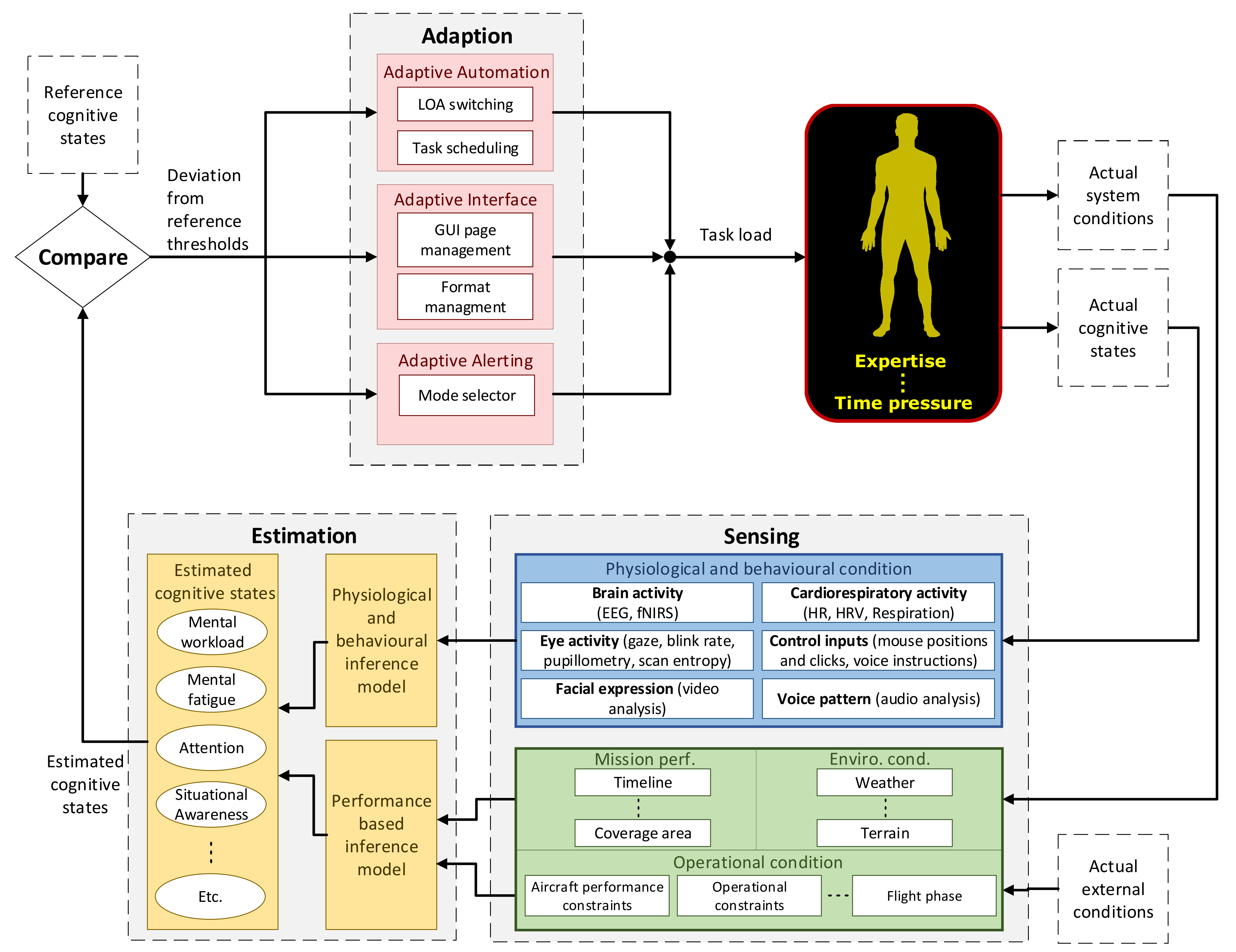
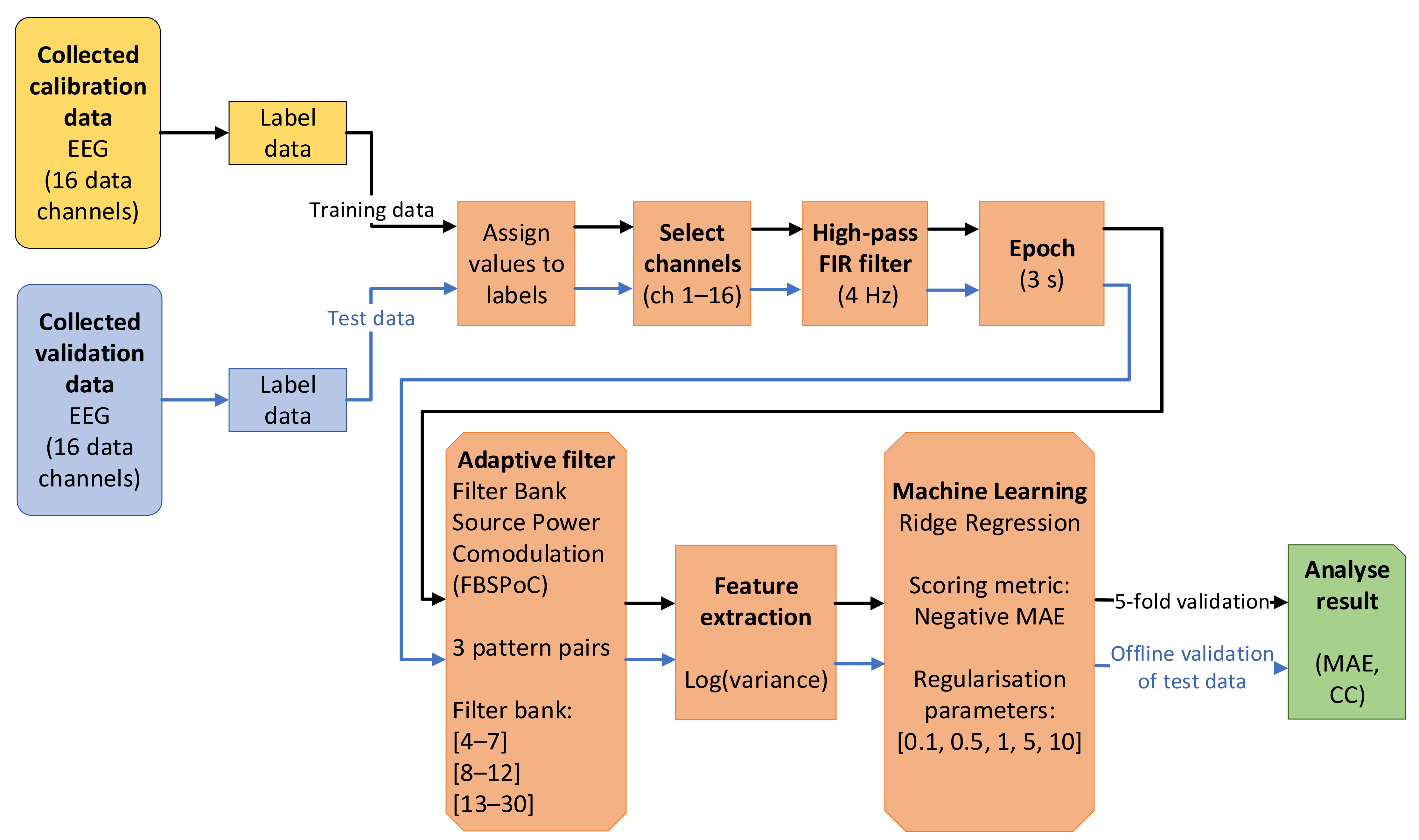
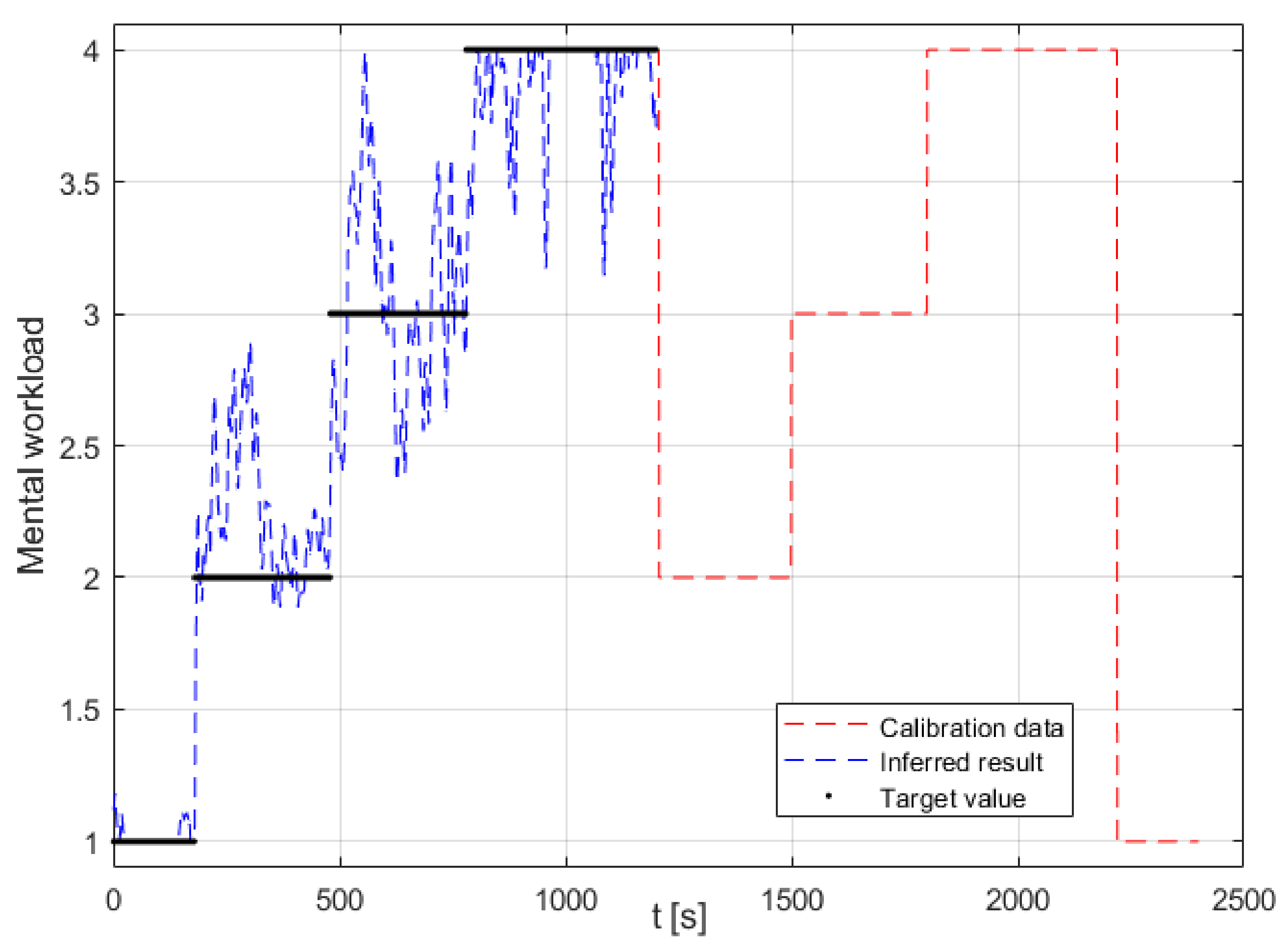
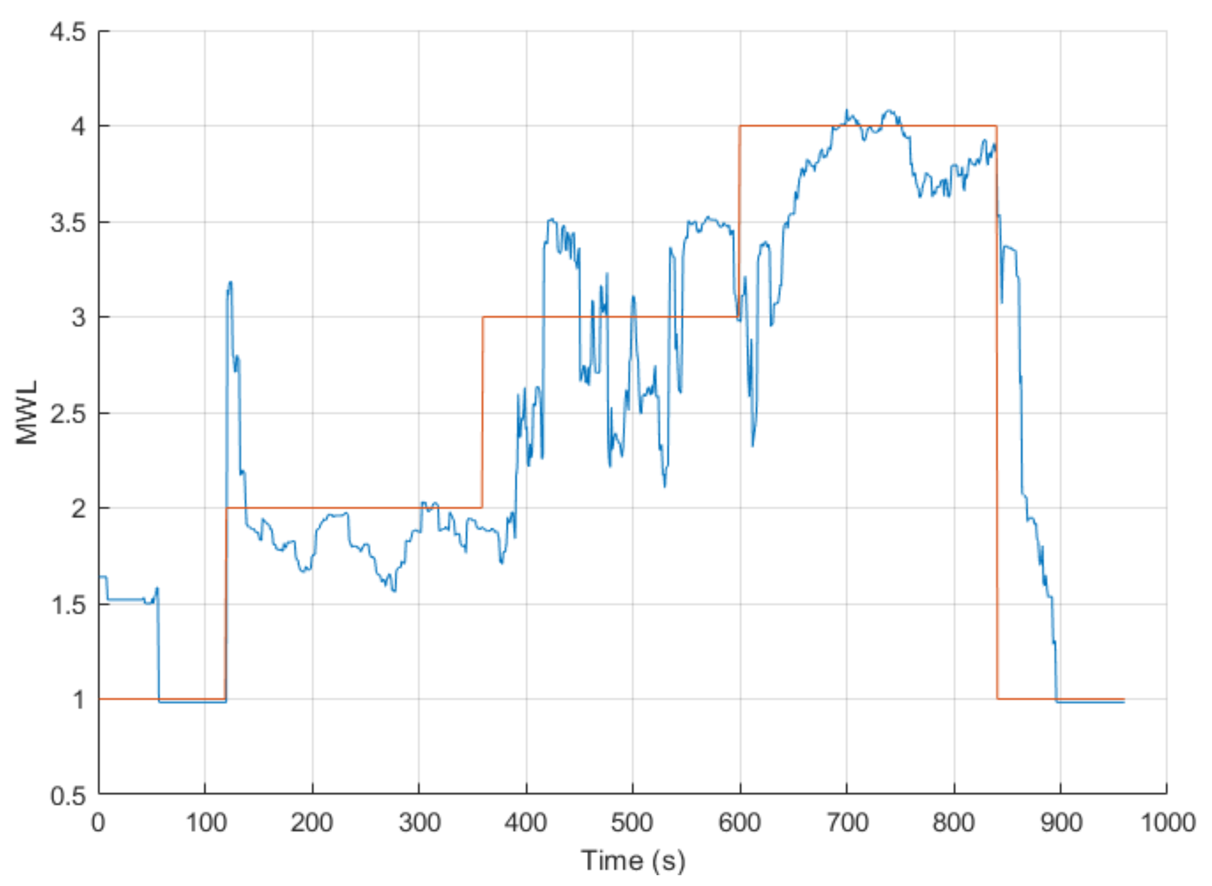
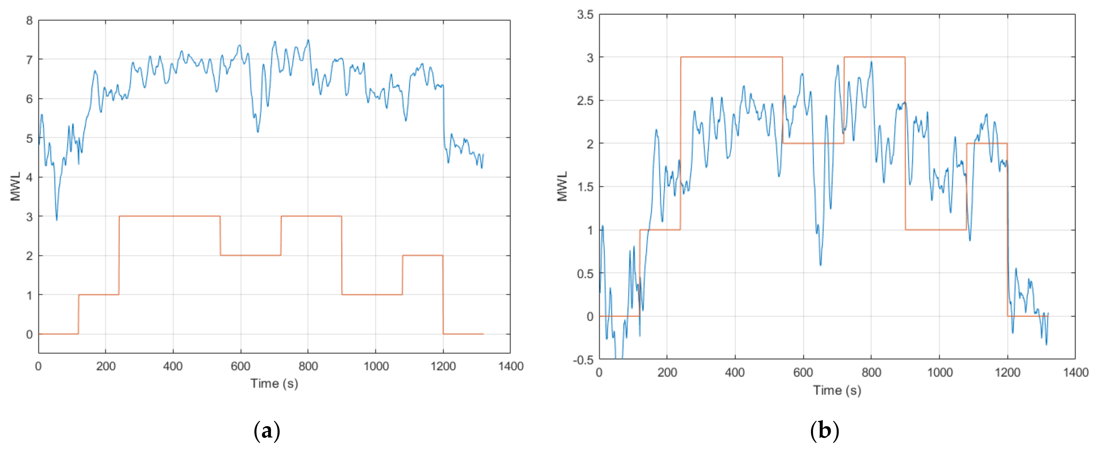
Figure 2.
Task load profiles for Session 1 and Session 2.
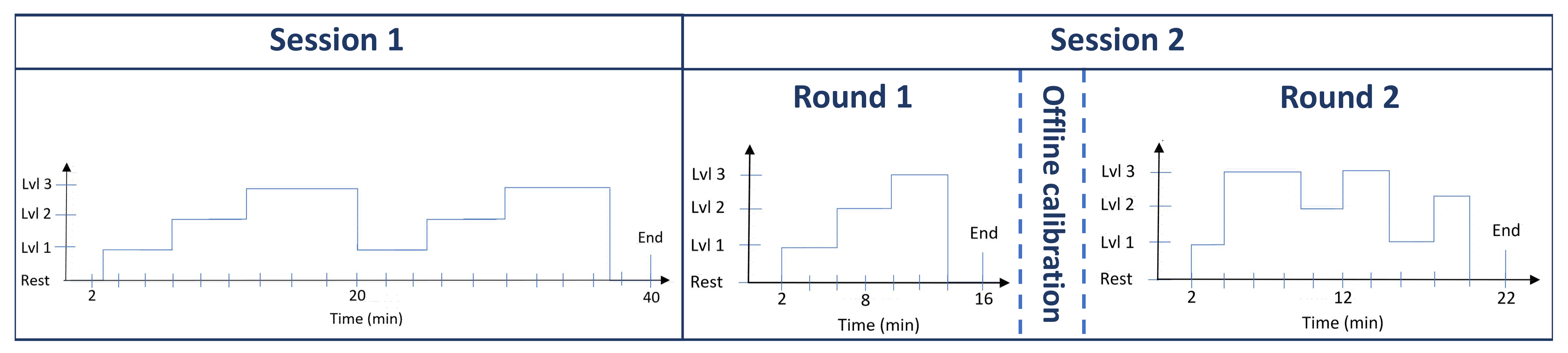
Figure 3.
Pipeline used for calibration and validation of the EEG model.

Figure 4.
Calibration and validation methodology for the multimodal ANFIS model.
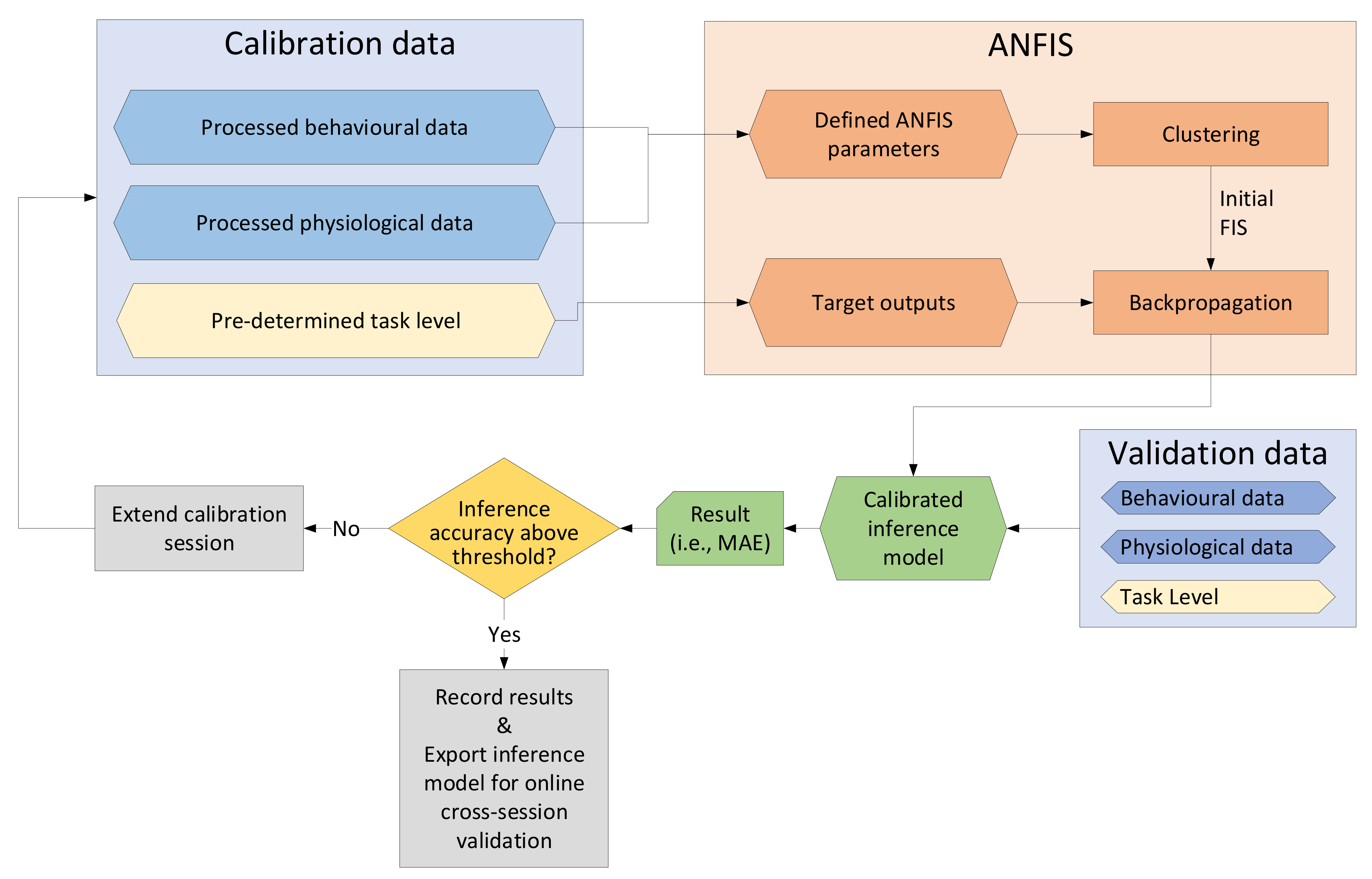
Figure 5.
Result from offline calibration and validation on separate halves of the data set. Red line indicates the section of data used for calibrating the ANFIS model, the black line is the target value that the model used for calculating the error and the blue line is the inferred result at one second intervals. The results shown here are from calibrating and validating on all seven applicable features for one participant (MAE = 0.196).

Figure 6.
Result from ANFIS model 2 for participant 5 (MAE = 0.37). Task level (red) and ANFIS model output (blue).
Figure 6.
Result from ANFIS model 2 for participant 5 (MAE = 0.37). Task level (red) and ANFIS model output (blue).

Figure 7.
Online EEG model output for participant 6 in Round 2. Task level (red) and EEG model output (blue): (a) The actual online output in relation to the task level with a MAE = 4.41; (b) EEG model output after adjusting for the offset resulting in a MAE = 0.61.
Figure 7.
Online EEG model output for participant 6 in Round 2. Task level (red) and EEG model output (blue): (a) The actual online output in relation to the task level with a MAE = 4.41; (b) EEG model output after adjusting for the offset resulting in a MAE = 0.61.

Figure 8.
Results from online multimodal fusion in Round 2. Task level (blue) and ANFIS models output (red): (a) output from ANFIS model 11 for participant 7 with MAE = 0.49; (b) output from ANFIS model 3 for participant 2 with MAE = 0.50.
Figure 8.
Results from online multimodal fusion in Round 2. Task level (blue) and ANFIS models output (red): (a) output from ANFIS model 11 for participant 7 with MAE = 0.49; (b) output from ANFIS model 3 for participant 2 with MAE = 0.50.
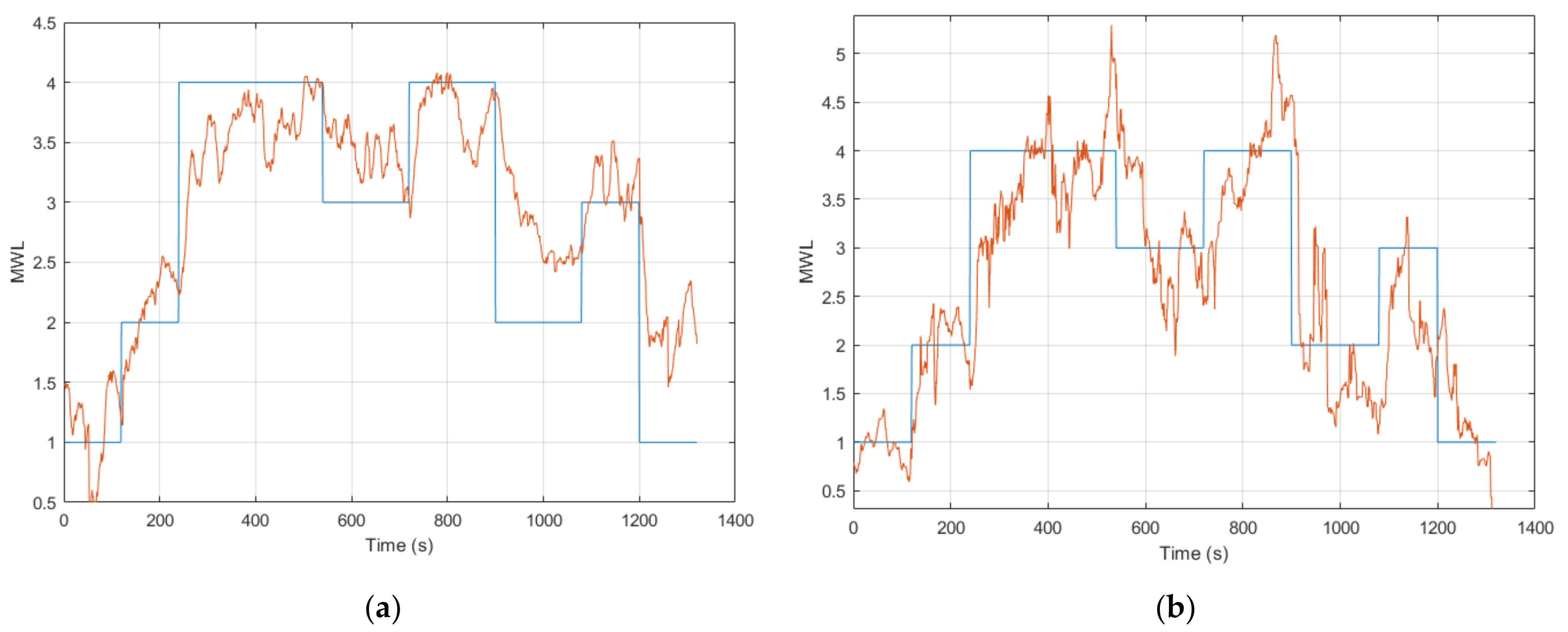
Table 1.
Results from the EEG model averaged across all 17 participants.
| Five-Fold Validation on First Half | Validation on Second Half of Unseen Data | Five-Fold Validation on All the Data | |
|---|---|---|---|
| Average MAE | 0.47 ± 0.09 | 0.81 ± 0.38 | 0.60 ± 0.10 |
Table 2.
Average pairwise correlation across all 17 participants.
| EEG | SPE | BPM | DIA | DWELL | HR | CI | |
|---|---|---|---|---|---|---|---|
| Average | 0.75 | 0.77 | −0.45 | 0.48 | −0.55 | 0.31 | 0.82 |
| CC | ±0.08 | ±0.08 | ±0.30 | ±0.44 | ±0.10 | ±0.18 | ±0.03 |
Table 3.
Results from offline calibration and validation from the 11 selected ANFIS models.
| ANFIS No. | Comment | Feature Combination | Average MAE |
|---|---|---|---|
| ANFIS 1 | Eye and CI option 1 | SPE, DIA, CI | 0.32 ± 0.05 |
| ANFIS 2 | Eye and CI option 2 | SPE, CI | 0.31 ± 0.05 |
| ANFIS 3 | Eye and CI option 3 | SPE, DIA, BPM, DWELL, CI | 0.38 ± 0.08 |
| ANFIS 4 | Eye and CI option 4 | SPE, DIA, DWELL, CI | 0.34 ± 0.05 |
| ANFIS 5 | Only eye features | SPE, DIA, BPM, DWELL | 0.51 ± 0.15 |
| ANFIS 6 | Best generic 1 | EEG, SPE, DIA, CI | 0.30 ± 0.07 |
| ANFIS 7 | Best generic 2 | EEG, SPE, CI | 0.32 ± 0.06 |
| ANFIS 8 | All 7 | EEG, SPE, CI, DIA, BPM, DWELL, HR | 0.36 ± 0.10 |
| ANFIS 9 | All 6 (no CI) | EEG, SPE, DIA, BPM, DWELL, HR | 0.45 ± 0.13 |
| ANFIS 10 | Lowest error (no CI) | Subject specific combination (Without CI) | 0.36 ± 0.09 |
| ANFIS 11 | Lowest error | Subject specific combination (With CI) | 0.28 ± 0.05 |
Table 4.
Results from online cross-session validation of ANFIS models 1 to 5 in Round 1. Conducted for six participants that completed Session 1.
Table 4.
Results from online cross-session validation of ANFIS models 1 to 5 in Round 1. Conducted for six participants that completed Session 1.
| ANFIS 1 | ANFIS 2 | ANFIS 3 | ANFIS 4 | ANFIS 5 | |
|---|---|---|---|---|---|
| Average | 0.72 | 0.63 | 0.74 | 0.67 | 0.74 |
| MAE | ±0.22 | ±0.23 | ±0.13 | ±0.16 | ±0.17 |
Table 5.
Average pairwise correlation across all 12 participants.
| EEG | SPE | BPM | DIA | DWELL | CI | |
|---|---|---|---|---|---|---|
| Average | 0.82 | 0.73 | −0.72 | 0.50 | −0.39 | 0.66 |
| CC | ±0.07 | ±0.15 | ±0.08 | ±0.33 | ±0.33 | ±0.13 |
Table 6.
Average MAE and CC between the online EEG inference and task level in Round 2.
| MAE | MAE * | CC | |
|---|---|---|---|
| Average | 3.04 ± 2.47 | 1.06 ± 0.31 | 0.54 ± 0.24 |
* MAE after adjusting for offset.
Table 7.
Average pairwise correlation across all 12 participants in Round 2.
| EEG | SPE | BPM | DIA | DWELL | CI | |
|---|---|---|---|---|---|---|
| Average | 0.54 | 0.67 | −0.70 | 0.54 | −0.53 | 0.58 |
| CC | ±0.25 | ±0.06 | ±0.08 | ±0.30 | ±0.08 | ±0.13 |
Table 8.
Results from online validation of all ANFIS models tested in Round 2.
| Participant | 1 | 2 | 3 | 4 | 5 | 6 | 7 | 8 | 9 | 10 | 11 | 12 | Average MAE | Average CC |
|---|---|---|---|---|---|---|---|---|---|---|---|---|---|---|
| MAE | ||||||||||||||
| ANFIS 1 | 0.60 | 0.51 | 0.89 | 0.77 | 0.55 | 0.69 | 0.48 | 0.70 | 0.62 | 0.82 | 0.51 | 0.67 | 0.65 ± 0.13 | 0.67 ± 0.12 |
| ANFIS 2 | 0.58 | 0.69 | 1.15 | 0.65 | 0.46 | 0.67 | 0.53 | 0.69 | 0.58 | 0.86 | 0.61 | 0.66 | 0.68 ± 0.18 | 0.66 ± 0.09 |
| ANFIS 3 | 0.55 | 0.51 | 0.87 | 1.05 | 0.45 | 0.59 | 0.49 | 0.75 | 0.59 | 0.71 | 0.57 | 0.86 | 0.67 ± 0.18 | 0.71 ± 0.15 |
| ANFIS 4 | 0.41 | 0.50 | 0.72 | 1.31 | 0.50 | 0.72 | 0.60 | 0.77 | 0.57 | 0.90 | 0.58 | 0.65 | 0.69 ± 0.24 | 0.61 ± 0.33 |
| ANFIS 5 | 0.59 | 0.60 | 0.73 | 1.55 | 0.53 | 0.59 | 0.55 | 0.75 | 0.62 | 0.78 | 0.68 | 0.87 | 0.74 ± 0.28 | 0.66 ± 0.22 |
| ANFIS 6 | 0.60 | 2.11 | 5.35 | 1.42 | 0.90 | 0.84 | 0.50 | 0.85 | 2.32 | 2.73 | 0.64 | 0.78 | 1.59 ± 1.40 | 0.69 ± 0.09 |
| ANFIS 7 | 0.63 | 2.42 | 1.20 | 1.44 | 0.53 | 1.80 | 0.51 | 0.76 | 2.51 | 0.99 | 0.61 | 0.68 | 1.17 ± 0.72 | 0.61 ± 0.26 |
| ANFIS 8 | 0.51 | 0.68 | 2.48 | 1.21 | 0.63 | 1.56 | 0.48 | 0.76 | 2.41 | 3.22 | 0.53 | 0.72 | 1.27 ± 0.94 | 0.64 ± 0.23 |
| ANFIS 9 | 0.59 | 2.01 | 3.01 | 1.20 | 0.87 | 0.91 | 0.52 | 0.69 | 1.53 | 4.47 | 1.30 | 1.91 | 1.51 ± 1.16 | 0.68 ± 0.19 |
| ANFIS 10 | n/a | 1.50 | n/a | 1.20 | 0.91 | 1.81 | 0.47 | n/a | n/a | n/a | n/a | n/a | 1.18 ± 0.52 | 0.72 ± 0.20 |
| ANFIS 11 | n/a | 1.58 | n/a | 1.28 | 0.72 | 0.69 | 0.49 | n/a | n/a | n/a | n/a | n/a | 0.95 ± 0.46 | 0.77 ± 0.06 |
Publisher’s Note: MDPI stays neutral with regard to jurisdictional claims in published maps and institutional affiliations. |
© 2021 by the authors. Licensee MDPI, Basel, Switzerland. This article is an open access article distributed under the terms and conditions of the Creative Commons Attribution (CC BY) license (https://creativecommons.org/licenses/by/4.0/).
Share and Cite
MDPI and ACS Style
Planke, L.J.; Gardi, A.; Sabatini, R.; Kistan, T.; Ezer, N. Online Multimodal Inference of Mental Workload for Cognitive Human Machine Systems. Computers 2021, 10, 81. https://0-doi-org.brum.beds.ac.uk/10.3390/computers10060081
AMA Style
Planke LJ, Gardi A, Sabatini R, Kistan T, Ezer N. Online Multimodal Inference of Mental Workload for Cognitive Human Machine Systems. Computers. 2021; 10(6):81. https://0-doi-org.brum.beds.ac.uk/10.3390/computers10060081
Chicago/Turabian StylePlanke, Lars J., Alessandro Gardi, Roberto Sabatini, Trevor Kistan, and Neta Ezer. 2021. "Online Multimodal Inference of Mental Workload for Cognitive Human Machine Systems" Computers 10, no. 6: 81. https://0-doi-org.brum.beds.ac.uk/10.3390/computers10060081
Note that from the first issue of 2016, this journal uses article numbers instead of page numbers. See further details here.