
Uncertainty-Aware Deep Learning-Based Cardiac Arrhythmias Classification Model of Electrocardiogram Signals


Department of Computer Science, College of Computer Engineering and Sciences, Prince Sattam Bin Abdulaziz University, Al-Kharj 11942, Saudi Arabia
Computers 2021, 10(6), 82; https://0-doi-org.brum.beds.ac.uk/10.3390/computers10060082
Submission received: 3 June 2021
/
Revised: 15 June 2021
/
Accepted: 16 June 2021
/
Published: 17 June 2021
(This article belongs to the Special Issue Advanced Methods for Information Extraction in Medicine and Space Biology)
Abstract
:Deep Learning-based methods have emerged to be one of the most effective and practical solutions in a wide range of medical problems, including the diagnosis of cardiac arrhythmias. A critical step to a precocious diagnosis in many heart dysfunctions diseases starts with the accurate detection and classification of cardiac arrhythmias, which can be achieved via electrocardiograms (ECGs). Motivated by the desire to enhance conventional clinical methods in diagnosing cardiac arrhythmias, we introduce an uncertainty-aware deep learning-based predictive model design for accurate large-scale classification of cardiac arrhythmias successfully trained and evaluated using three benchmark medical datasets. In addition, considering that the quantification of uncertainty estimates is vital for clinical decision-making, our method incorporates a probabilistic approach to capture the model’s uncertainty using a Bayesian-based approximation method without introducing additional parameters or significant changes to the network’s architecture. Although many arrhythmias classification solutions with various ECG feature engineering techniques have been reported in the literature, the introduced AI-based probabilistic-enabled method in this paper outperforms the results of existing methods in outstanding multiclass classification results that manifest F1 scores of 98.62% and 96.73% with (MIT-BIH) dataset of 20 annotations, and 99.23% and 96.94% with (INCART) dataset of eight annotations, and 97.25% and 96.73% with (BIDMC) dataset of six annotations, for the deep ensemble and probabilistic mode, respectively. We demonstrate our method’s high-performing and statistical reliability results in numerical experiments on the language modeling using the gating mechanism of Recurrent Neural Networks.
1. Introduction
Artificial Intelligence (AI) has become increasingly influential in the healthcare system, yielding robust evaluations and reliable medical decisions. The vast availability of biomedical data brings tremendous opportunities for advanced healthcare research, particularly the subdomain related to the monitoring of patients. The success of Deep Neural Networks (DNNs) in the analysis and diagnosis of complex medical problems has demonstrated a remarkable performance, making it one of the most effective solutions in the medical domain. Methods for cardiac dysfunction diseases have benefited from the advancement of DNNs by exploiting the enormous heterogeneous biomedical data to improve conventional clinical diagnosis methods, including the detection and classification of heart dysfunctions.
AI-assisted decision-making applications are now increasingly employed for analyzing and classifying cardiac dysfunctions employing electrocardiographic morphology readings [1,2,3,4,5]. Cardiac dysfunctions are anomalies in the heart’s electrical impulses records, including cardiac arrhythmias, which can be analyzed and diagnosed from electrocardiogram recording. The electrocardiogram (ECG) has been widely recognized as one of the most reliable and noninvasive methods for monitoring heart rhythms. An ECG records impulses to manifest the heartbeat patterns, rhythm, and strength of these impulses as they impel through the heart during a time interval so that abnormal changes within an ECG recording would signify heart-related conditions. As manual heartbeat classification of the long-term ECG recordings can be very time-consuming and needs much more practice, with an AI-powered automated recognition and classification system of ECG recordings yields an efficient and accurate diagnosis, ultimately improving the quality of medical treatment.
Machine learning-based solutions operate on the deterministic point-estimate mode, meaning that they do not quantify the uncertainty of the model’s predictions, leading to potential imprecision during results interpretation. In general, the performance of machine learning models is usually evaluated in terms of metrics related to the models’ discriminative power, such as accuracy and F1-score. However, it is sometimes crucial to verify the model’s uncertainty about its predictions, especially in the medical domain where diagnostic errors are inadmissible. There have been quite some works in quantifying the uncertainty estimations in machine learning methods. Fuzzy-based methods have been used to provide problem-tailored uncertainty estimation solutions for classification and clustering tasks [6,7,8]. Bayesian-based probabilistic methods have been primarily leveraged for the uncertainty estimations of deep neural networks [9,10,11]. This work employs the latter approach for the task of uncertainty quantifications.
Motivated by the desire to introduce an AI-powered broad-spectrum cardiac arrhythmias classification design, this paper introduces an uncertainty-aware predictive model for cardiac arrhythmias classification structured using carefully engineered Gated Recurrent Neural Networks (GRUs) architecture that is trained using three publicly available medical datasets and capable of classifying the most extended set of annotations (up to 20 different types of arrhythmias annotations), yielding the uttermost possible classification performance that is known to us. Moreover, we apply an easy-to-use feature extraction method, namely the moving window-based method, to fragment prolonged electrocardiogram recordings into multiple segments based on provided annotations. In addition, considering that DNN-based methods tend to be overconfident [12,13], the introduced design estimates the model uncertainty about its outputs using a Bayesian-based approximation method, namely Monte Carlo-based dropout, without introducing additional parameters or significant changes to the network’s architecture, assessed using a safety-specific set of metrics to interpret the models’ confidence concerning the safety-critical domain applications. By applying such an uncertainty quantification, the presented model could be exploited to mimic the clinical workflow and transfer uncertain samples to additional analysis. Simply put, the contribution of this work can be summarized into two folds:
- The ability to outperform the existing results by being able to classify the most extensive set of ECG annotations that are known to us (reaching 20 different imbalanced sets of annotations) in high results.
- The successful incorporation of model uncertainty estimation technique to assist the physician-machine decision making, thus improving the performance regarding the cardiac arrhythmias diagnosis.
This work attempts to present the best possible AI-assisted decision-making cardiac arrhythmias classification model to improve the performance of arrhythmias diagnostics, potentially in deployable real-world settings. The rest of this paper is organized as follows: Section 2 presents the preliminaries of the essential elements used in this paper. Section 3 describes the datasets used during the experiment, followed by demonstrating the paper’s proposed method. The paper’s experiment is thoroughly presented in Section 4 followed by a discussion of the results in Section 5. The related works are presented in Section 6. The paper is finally concluded in Section 7.
2. Preliminaries
To cover every aspect, we provide a concise and brief discussion of the electrocardiogram signals (ECGs) from the medical point of view to help the reader understand the fundamental concepts of ECGs. Moreover, we briefly discuss the Gated Recurrent Neural Network (Gated RNNs), a class of artificial neural networks designed for sequential and time-series data, which is mainly used in this experiment.
2.1. Electrocardiogram (ECG)
An electrocardiogram records the heart’s electrical activity against time, where the changes in the electrical potential difference during depolarization and repolarisation of the cardiac muscle are recorded and monitored [14]. ECG provides accurate and immediate interpretations of various cardiac pathologies at a low cost, making them the best non-invasive choice to diagnose abnormal cardiac conditions in a real-time manner.
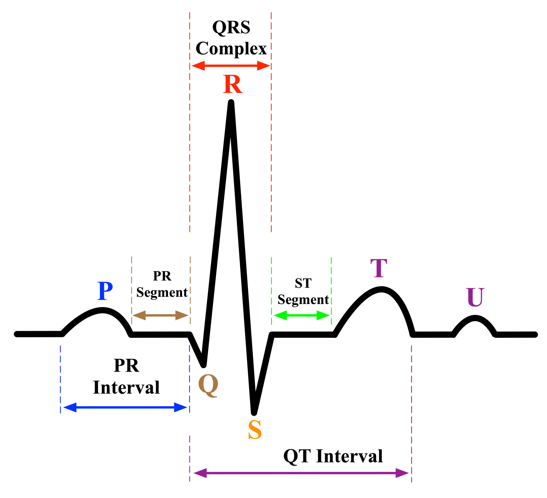
ECG signal analysis has been a subject of study for many years. It is the fundamental analysis for the interpretation of the cardiac rhythm. In a nutshell, an ECG waveform consists of three main elements: waves, segments, and intervals, as shown in Figure 1. First, waves are the deflections from the baseline (positive or negative) indicating an electrical event. The essential waves on the ECG waveform are P, Q, R, S, T, and U waves. The P wave represents atrial depolarization [15,16]. The Q, R, and S waves, commonly known as QRS complex, represent the ventricular depolarization and they are calculated by the sum of the electrical activity of the inner (endocardial) and the outer (epicardial) cardiac muscles [17]. T wave represents the repolarization of ventricle [15,16]. Second, segments are the length between two specific points on an ECG. The segments on an ECG include the PR, ST, and TP segments. Third, intervals are the time between two ECG events. The intervals on an ECG include the PR, QRS, QT interval, and RR intervals. The QRS complex is considered the main feature in diagnosing many cardiac pathologies [18]. The quality of the detection of ECG waveform characteristics is based on accurately detecting the QRS complex and the P and T waves (P-QRS-T) because they can easily lead to identifying more detailed information such as the heart rate, the ST segment, and more [19]. This is usually done by physicians analyzing the ECG signals recorded simultaneously at different human body points to identify diagnostics related to heart functioning accurately.
2.2. From Recurrent Neural Networks (RNN) to Gated Recurrent Units (GRU)
Before elaborating on the Gated Recurrent Neural Networks (or Gated Recurrent Units (GRU) for short), we first discuss Recurrent Neural Network (RNN) as being the origin. Recurrent Neural Networks are fundamentally designed to process data streams of arbitrary length by recursively applying a transition function to its hidden internal states for each input sequence [20]. RNNs can handle variable-length sequences by making recurrent hidden states whose current activation output depends on the previous one to handle long dependencies. Because RNNs have been successful with sequential data, they are well suited for the health informatics domain, where immense amounts of sequential data are available [21].
Formally, given a sequence , a default RNN updates a recurrent hidden state at time t as [22]:
it is common to choose f as a nonlinear activation function, such as sigmoid or tanh, with an affine transformation of both and . Thus, the update of the recurrent hidden state can be rewritten as:
where is m-dimensional input vector at time t, is n-dimensional hidden state, is a nonlinear activation function, W is weight matrix of size , U is recurrent weight matrix of size , and b is a bias of size .
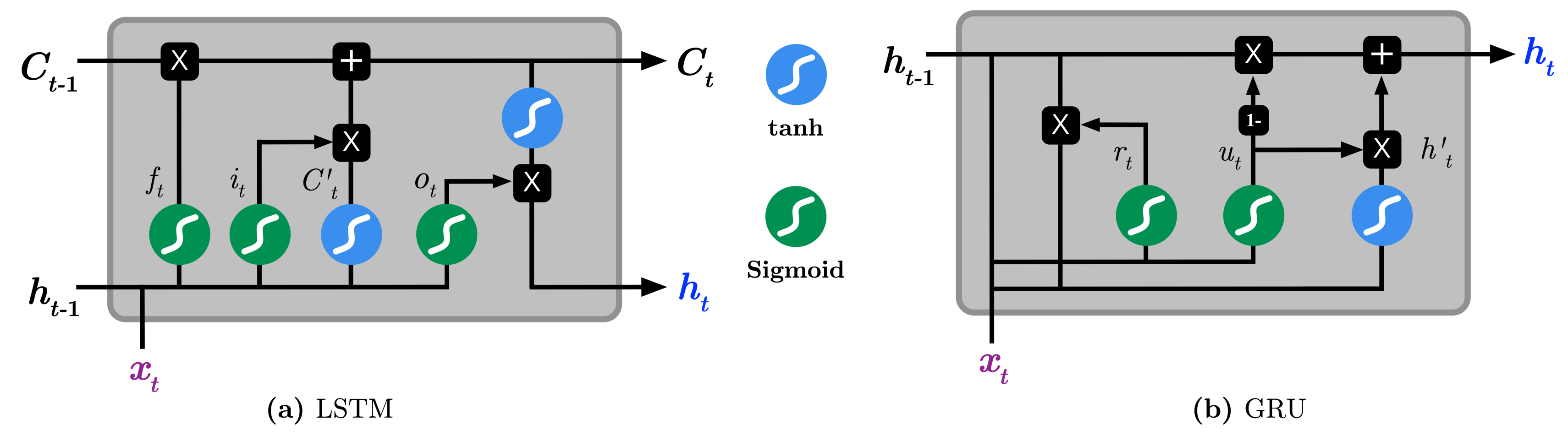
It was observed that the default RNN is deficient in capturing long-term dependencies because the gradients tend to either vanish or explode with long sequences [23]. As a consequence, two RNN variations, namely the Long Short Term Memory (LSTM) [24,25] and, most recently, Gated Recurrent Units (GRU) [23,26], have been introduced to resolve the vanishing and exploding gradient problems. Both variations have the similar goal of keeping long-term dependencies effective while alleviating the vanishing and exploding gradient problems. As seen in Figure 2, LSTMs essentially consists of three gates: input gate , forget , output , input vector , and an output activation function. The key element in LSTM is the cell state , which enables the information to flow along the cell unchanged. The input gate regulates which value should be updated, the forget gate regulates which value of the cell state should be forgotten, and the output gate regulates how much information should be transformed to the next layers of the network. To summarize, the following Equations briefly describe the operations performed by the default LSTM [22]:
where denotes the input at time t, are weight matrices, is the bias term, is the sigmoid function, the · denotes component-wise multiplication, and is the output gate. Finally, the hidden state constitutes the value of the output gate at time t being point-wise multiplied with the nonlinearly transformed cell state , and it is calculated by:
On the other hand, GRUs operate using only reset and update gates. It essentially combines the forget and input gates into the update gate and merges the cell state and hidden state into the reset gate. The resulting architecture appears simpler hence less training parameters are needed than LSTM, making the training faster than LSTM [23]. The operations performed by the GRU model is as follows:
where and are respectively the reset and update gates at time t, are weight matrices, and · denotes component-wise multiplication.
2.3. Uncertainty in Neural Networks
The combination of Bayesian statistics and neural networks implies uncertainty estimation in the learning model predictions, introducing Bayesian Neural Networks (BNNs) [27]. The Bayesian Neural Network (or Bayesian Deep Learning) is essentially a stochastic neural network trained using the Bayesian inference model. The essence of BNN is to capture uncertainty in the model by inferring a probability distribution over the model’s weights instead of point estimates. It adds a prior distribution over the model’s weights and then attempts to capture how these weights vary given some data. There are two main types of uncertainty one can model [28]. First, aleatoric uncertainty measures noise inherent in observations from the environment’s dynamics, which typically appears during the data collection method, such as motion noise or sensor noise, making it harder to reduce even with enough data. Second, epistemic uncertainty (model uncertainty) looks for uncertainty in the model parameters. This type is difficult to model since it requires placing a probability distribution over the entire model parameters to capture how much these weights vary given some data. Simply put, epistemic uncertainty is modeled by placing a prior distribution over the model’s weights and then trying to capture how much these weights vary given some data while aleatoric uncertainty is modeled by placing a distribution over the model’s output.
In the typical neural network setting, the task is to find the optimal weights as an optimization problem to be solved using an optimization method such as stochastic gradient descent in order to obtain a set of and a single prediction of . On the other hand, BNN differs from the previous setting as it tries to learn a distribution over the model’s weights and subsequently the predictive posterior distribution of using the Bayesian inference model. Formally, given input data , Bayesian modeling allows to capture model uncertainty by estimating the posterior distribution over the weights as the following:
where is the likelihood function of , is the prior over weights, and is the marginal likelihood (evidence). The calculation of the posterior is often intractable because computing the marginal likelihoods usually requires computing very high-dimensional integrals. Several approximation techniques have been introduced to overcome such intractability, including Markov Chain Monte Carlo (MCMC) sampling-based probabilistic inference [9,29], Laplace approximation [30], variational inference [10,27,31], and Monte Carlo dropout inference [11].
3. Materials and Methods
This section explains the datasets used during the experiment, followed by describing the proposed preprocessing approach applied on the dataset, the modeling, and uncertainty estimation.
3.1. Data Description
As stated before, this experiment aims to construct a practical cardiac arrhythmias classification model using reliable and reputable electrocardiogram (ECGs) datasets. We will be using three publicly available arrhythmia datasets provided by the PhysioBank, hosted by the PhysioNet repository and managed by the MIT Laboratory for Computational Physiology: (1) MIT-BIH Database [32,33], (2) St Petersburg INCART Database [32], and (3) BIDMC Database [34]. The databases use a standard set of annotation definitions (i.e., codes) standardized by PhysioNet [35]. Annotations are nothing but a labeling strategy to characterize particular locations within an ECG recording to describe events at those locations. It is worth noting that these standard sets of annotation codes are divided into two categories: beats annotations and non-beats annotations. The beats annotations identify heartbeats, and they have a specific meaning, while non-beats annotations describe the non-beat events and can take another set of values (The description of the standard set of annotation codes used by PhysioBank can be found https://archive.physionet.org/physiobank/annotations.shtml, accessed on 17 June 2021).
3.1.1. MIT-BIH Database
This database has been considered to be the benchmark database for arrhythmia analysis and electrocardiogram signal processing. It contains 48 records of two-channel ambulatory ECG recordings (signals), sampled at 360 samples per second with 11-bit resolution from 47 subjects. In most records, the upper signal is the modified-lead II (MLII), while the lower signal is usually a modified lead V1, V2, V4, or V5, depending on the record. Since the normal QRS complexes are eminent in the upper signal, we only process the upper ECG signal of each record. The upper ECG signal has been annotated independently by two or more cardiologists, with the disagreements being reviewed and resolved by consensus. Thus, the total number of annotations in all records of this database is annotations, as seen in Table 1a. Accordingly, we process this database for the classification task by constructing three datasets of different labeling levels. First, we form a dataset by considering all possible sets of annotations from the recordings, except we drop (`S’, ‘]’, and ’[’) annotations because there are few samples for them, consequently forming a dataset of 20 classes. Second, we form a dataset by considering the beats-only annotations from the recordings, except we drop ‘S’ annotation because there are few samples for it, consequently forming a dataset of 14 classes. Third, we form a dataset by considering a specific set of classes proposed by the Association for Medical Instrumentation Advancement AAMI [36], which recommends grouping the original 15 heartbeat types, i.e., beats-only annotations, into five superclasses beats: normal (N), ventricular ectopic beat (VEB), supraventricular ectopic beat (SVEB), fusion beat (F), and unknown beat (Q), as shown in Table 1b, consequently forming a dataset of 5 classes.
3.1.2. St Petersburg INCART Database
This database includes 75 recordings from 32 subjects obtained by Holter records. Each record is 30 about minutes long and contains 12 standard leads, sampled at 257 samples per second. The records are annotated following the standard PhysioBank beats annotation using an automatic algorithm followed by manual corrections. Thus, the total number of annotations in this database is 175,720 annotations, as shown in Table 1a. We process this database for the classification task by forming a dataset using all possible sets of annotations from the recordings, except we drop (`Q’, ‘+’, ‘B’) annotations because there are few samples for them, consequently forming a dataset of 8 classes.
3.1.3. BIDMC Database
This database includes 15 long-term recordings, each of which contains two ECG signals sampled at 250 samples per second with 12-bit resolution from 15 subjects with severe congestive heart failure. We process the upper ECG signal of each record. As seen in Table 1a, this database contains in total 1,622,493 annotations, where almost of the annotations are being normal ‘N’. Hence, we only choose 200 K of ‘N’ annotation during this experiment. In addition, we process this database for the classification task by considering a single dataset of all possible sets of annotations from the recordings except we drop ‘E’ annotation because there are few samples for it, consequently forming a dataset of 6 classes.
3.2. Signal Segmentation
Before elaborating on the processing pipeline, we first explain the segmentation method used for ECG long-term recordings. As described in the previous section, the QRS complex is the most significant spike in the ECG signal because it represents the cardiac ventricular muscles’ conditions, which can be used to diagnose several diseases [17,37]. The prominent characteristics of the QRS complex are the amplitude of the R wave, the duration of the QRS complex, and the RR interval (RR interval refers to the time between two consecutive R peaks). All databases used in this experiment are annotated using a predefined set of annotations, and therefore we want to construct a labeled dataset from each database recording. To do so, we process each raw ECG record using its provided annotation in the following steps:
- Locate QRS locations in the record.
- Extract the corresponding segments using the moving window approach.
- Label the extracted segments using their corresponding annotations.
The moving window-based segmentation approach is illustrated in Figure 3. The segmentation is performed by first locating a QRS complex at a location, say i, and subsequently advance one second in both directions, and , to ensure the extraction of the essential waves, i.e., P wave, QRS complex, T wave, within the location, hence producing a segment . It is worthwhile to mention that the standard QRS duration is relatively between 0.06 to 0.12 s [37,38]; therefore, we selected the window’s length precisely one second to be long enough to cover the time duration of abnormal QRS complexes but short enough not to overlap both QRS complex and T wave as possible.
3.3. Processing Pipeline
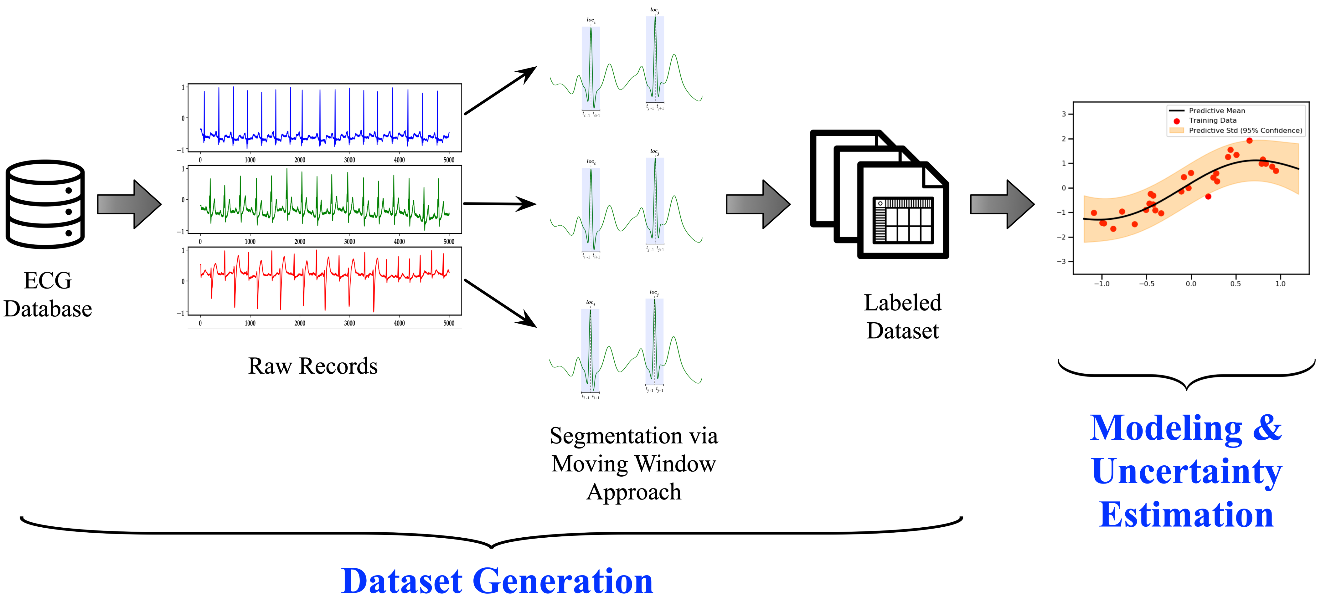
The processing pipeline for constructing a cardiac arrhythmia classification model is illustrated in Figure 4. It consists of two phases: (1) dataset generation and (2) modeling & uncertainty estimation. The process starts with taking the raw ECG records from the database and apply the segmentation approach explained formerly, yielding a labeled dataset ready to be used for modeling. Next, we begin modeling the dataset using a GRU-based Recurrent Neural Network method. In general, the Recurrent Neural Network (RNN) selection was intended because RNNs have been traditionally successful in signal processing, regardless of the extended training times and advanced hardware requirements usually required, especially when dealing with prolonged signals. In the end, the modeling step is followed by estimating the model’s uncertainty to capture the model’s level of confidence toward the unseen data.
3.4. Uncertainty Estimation
Neural network-based solutions operate on the deterministic and point-estimate mode, meaning that they do not quantify the uncertainty of the model’s predictions, leading to potential imprecision during results interpretation. In principle, DNN-based classification tasks yield a vector of probabilities (produced by a softmax transformation) for a set of classes being considered. When the probability for one class is considerably higher than the other probabilities, we often interpret it as correct with high confidence without rationalizing if the model is certain. In the context of machine learning-based modeling in the medical domain, it is crucial to know when the model is uncertain to avoid severe consequences. In other words, we want to know when the model does not know. This kind of reasoning is vital, especially for safety-critical applications.
Deep neural networks perform well on data that have been trained around before. The difficulty is that the training dataset often covers a minimal subset of the entire input space, making it challenging for the model to be decisive on new unseen data originating from a different space. In this case, the model will attempt to guess the new data class without providing any level of confidence. To assess the model’s confidence, we want to be able to quantify the model’s uncertainty against new data, and this can be effectively achieved using Bayesian inference via Bayesian Neural Network (BNN). However, Bayesian inference has been recognized to be computationally intensive due to the computational intractability of the marginal likelihood (evidence) in the model’s posterior.
Several studies have demonstrated that one can instead approximate the model posterior (inference approximation). Laplace approximation [30], variational inference [10,39], and most recently Monte Carlo dropout estimation method [11] are all approximation approaches intended to overcome the Bayesian inference’s computational complexity. Gal et al. [11] showed that the dropout regularization, a technique commonly used to control overfitting in DNNs, is equivalent to approximate the variational inference of the Bayesian model when it is applied during the testing phase. Therefore, this work employs model uncertainty estimation using the Monte Carlo dropout method (MC dropout) to quantify the model’s predictive uncertainty.
In the classification setting, the predictive uncertainty of an input sample is the entropy of the categorical softmax after calibration over the weight settings. In this work, we use predictive entropy to evaluate the quality of the uncertainty estimates. In practice, when applying dropout in a conventional neural network, each unit is randomly dropped with probability during training time. At the testing time, the dropout is turned off, meaning that the units are always present, and the weights are multiplied by . On the contrary, the dropout mechanism in the Monte Carlo method remains on during the test time and the prediction pass (i.e., forward pass through the network) is performed T times followed by averaging the results under the posterior distribution, thus estimating the predictive uncertainty. Formally expressed, given a dataset , the predictive distribution of the output given a new input is [40]:
the integral can be approximated using Monte Carlo sampling method [41] over T iterations as:
which is also called the predictive mean , and is the network’s weights having dropout turned on at the ith MC dropout iteration. For each test sample, the class with the largest predictive mean is selected as the output prediction. Ultimately, we capture the model uncertainty by computing the predictive entropy over K classes as the following:
where is the predictive means probability of ith class from T Monte Carlo samples. Thus, the higher predictive entropy corresponds to a greater degree of uncertainty, and vice versa.
4. Experimental Details
This section describes the models design and configuration followed by the evaluation metrics used to evaluate our proposed system.
4.1. Model Design and Configuration
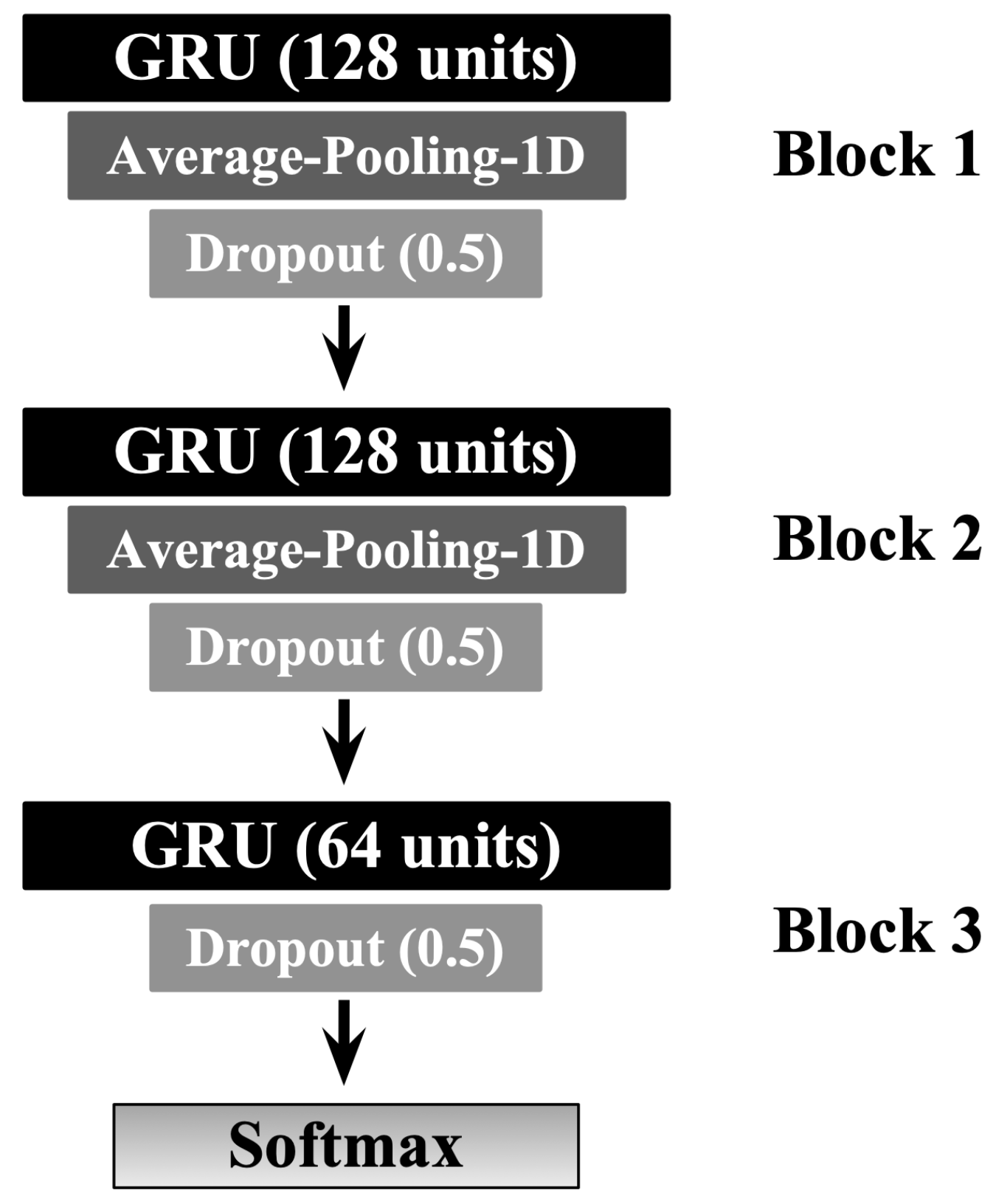
In this work, we applied the Gated Recurrent Neural Networks (or Gated Recurrent Units (GRU) for short) method to be used for the classification task. We spent quite an amount of time experimenting with varying GRU-based architectures and hyperparameters tuning choices to achieve the best possible results, including Figure 5 which demonstrates the best model design and configuration. The final GRU architecture consists of three GRU-based blocks, each of which is followed by a one-dimensional average pooling and a dropout layer. The pooling is to downsample the input representation by taking the average value over a defined-sized window called pool size and shifted forward by a particular value. In the dropout layer, individual nodes from the GRU netwrok are either dropped out with probability or kept with probability p. The experimental environment was implemented using TensorFlow v2.4.1 via the application programming interface Keras v2.4.1 [42,43]. The model training and prediction were performed on a workstation with an Intel Core i7-10700KF (3.8 GHz) CPU, Nvidia Geforce RTX 3060 Ti (8 GB) GPU, and 64 GB of RAM.
The objective of the neural network-based methods is to reduce the loss functions that measure the discrepancy between the predicted value and the true label. In our experiment, we have found out that ADAM optimizer [44], with the learning rate of , works well during the training and the validation phases. The learning rate is one crucial parameter that regulates how much change can be applied to the model in response to the estimated error when the model weights are updated [45]. The choice of activation functions used for the GRU’s update and reset gates were set to the sigmoid function, while the recurrent activation is set to the hyperbolic tangent function (tanh) (We shall release the source code for public use upon publication at https://github.com/DrAseeri/cardiac-arrhythmia-uncertainty-estimation, accessed on 17 June 2021).
4.2. Evaluation Metrics
The performance of machine learning-based methods is generally evaluated in terms of metrics related to the models’ discriminative power. Thus, we choose a set of metrics that accurately assess our models’ performance as a multiclass classifier. Given that the input datasets are highly imbalanced, we specifically employ the following metrics: Precision, Recall, F1-score, and the area under the receiver operating characteristic curve (AUROC). These metrics have been widely adopted for multiclass classification problems as they provide a deeper analysis of the model’s behavior toward each class.
Formally, the multiclass classification problem refers to assigning each data point into one of the K classes. The goal is to construct a function which, given a new data point, will correctly predict the class to which the new data point belongs to. Unlike the binary classification problems, there is no cut-off score (i.e., threshold) to make predictions. Instead, the predicted output is the class with the highest predicted value. Classically, the performance of a binary classification model can be evaluated by means of four features: the number of correctly identified class instances (true positives TP), the number of correctly identified instances that do not belong to the class (true negatives TN), and instances that either was incorrectly assigned to the class (false positives FP) or that were not recognized as a class instance (false negatives FN). In the case of a multi-class classification problem, this can be easily extended to cover a set of K classes as follows: given a class , is a set of true positives, is a set of true negatives, is a set of false positives, is a set of true negatives, the weighted average for each of the metrics mentioned above is calculated as follows [46]:
where in AUROC gathers all classes different from class i, meaning that AUROC is computed here using the one against all approach, i.e., we compute this measure as the average of k combinations.
4.3. Probabilistic-Based Metrics
The predicted classes are said to be either correct when the highest predicted values match the respective true classes or incorrect otherwise. However, there is no notion of knowing the model’s certainty toward the predicted classes, meaning that it solely follows the softmax predicted outputs and is often erroneously interpreted as model confidence. The authors in [11] show that a model can be uncertain in its predictions even with a high softmax output. A perfect system would correctly rate predictions as correct with higher confidence (low uncertainty) and incorrect predictions with low or no confidence (high uncertainty). Uncertainty estimation has been a challenging task since there is no ground truth available for the uncertainty estimates. Inspired by [47], we will evaluate uncertainty estimation of our proposed architecture using the following possible outcomes: correct and certain (CC), correct and uncertain (CU), incorrect and certain (IC), and incorrect and uncertain (IU). The most severe case is when the predictions are incorrect but the model is certain (IC), while an acceptable yet impractical model might correctly identify predictions but in relatively high uncertainty (CU). For such a system, the goal is to minimize the error from (1) the ratio of the number of certain but incorrect samples to all samples (IC), and (2) the ratio of the number of uncertain but correct samples to all samples (CU). Moreover, we also consider measuring the accuracy of the uncertainty estimates as the ratio of the optimal outcomes (i.e., correct and certain (CC) and incorrect and uncertain (IU)) over all possible outcomes, where the higher value (close to 1) indicates to the model that is in a perfect mode for most of the time.
More specifically, we evaluate the quality of predictive uncertainty estimates using conditional probability-based metrics across various uncertainty thresholds as proposed in [48]. These metrics require only the actual true labels, the model predictions, and the normalized uncertainty estimates . To do so, we first apply a threshold on the continuous uncertainty values of to split the predictions into two groups: certain when and uncertain when . Second, the resulted model predictions are divided into correct when the ground truth matches the predictions, and incorrect otherwise. Therefore, we can formulate the following conditional probabilities:
- P(correct|certain) indicates the probability that the model is correct on its outputs given that it is certain about its predictions. This can be calculated as:
- P(uncertain|incorrect) indicates the probability that the model is uncertain about its outputs given that it has produced incorrect predictions.
We also measure the accuracy of the uncertainty estimation (AU) as the ratio of the desirable cases (i.e., correct and certain, incorrect and uncertain) over all possible cases as the following:
Hence, a model with a higher value of the above metrics is considered a better performer. Please note that the above metrics are computed over a set of thresholds , meaning that we evaluate the model results using the above metrics on different thresholds and choose the best possible threshold value.
4.4. Data Oversampling
As shown in Table 1a, the class distribution (i.e., the distribution of heartbeat annotations) of all databases employed in this work is highly imbalanced. Therefore, we allow oversampling the minority classes by generating synthetic segments that belong to the under-represented classes using the Synthetic Minority Oversampling Technique (SMOTE), which is efficiently implemented by the imbalanced learn package [49]. Here we emphasize that oversampling is only performed on the training set, whereas the validation set and testing set remain intact so that the performance metrics can correctly deduce the results from the original class distribution.
5. Results and Discussion
In this section, we demonstrate and analyze the performance of our proposed design architecture discussed in Section 4.1 using the input datasets described in Section 3.1. All results shown are based on a separate test set used for neither training nor hyperparameter tuning. The proposed design in Section 4.1 is implemented in two modes: deep ensemble (DEs) [39] mode and Monte Carlo-based dropout (MCDO) mode. We employ the deep ensembles method in our experiment to demonstrate our proposed GRU-based deterministic power when applying the input datasets. To fully evaluate the effectiveness of the resulted models in both modes, we collect the classifier’s predictions and evaluate them using the general-purpose metrics previously described in Section 4.2. Moreover, the uncertainty estimates obtained from operating Monte Carlo-based dropout mode are evaluated using probabilistic-based safety-specific metrics discussed in Section 4.3 for reliable and informed decision making in safety-critical applications.
5.1. Deep Ensemble Performance
Deep Ensemble (DE) is a sampling-based approach used for estimating the predictive power of DNNs using an ensemble of neural networks [39]. In this approach, multiple models of different random initializations with the same underline architecture are trained, and their softmax outputs are averaged to obtain the predictive mean. Although the deep ensemble method is known to introduce additional complexity and overhead from training multiple models, it is used in our experiment as a stress test to assess the model’s performance. Table 2 illustrates the results of five-samples deep ensembles. It can be concluded that our proposed GRU-based architecture is successfully able to classify the annotations in each of the input datasets with very high performance. In addition, we plot in Figure A1 the multi-class ROC curves of the deep ensemble resulting from each input datasets in a different set of annotations (one-vs-all approach) (Due to the large number of plots in this work, we move them into the Appendix A at the end of this paper.). We can observe that the lowest AUC value is 0.95, meaning that the DE model in general can classify between the classes at a high rate.
5.2. Uncertainty Estimation Performance
We evaluate the quality of our models’ uncertainty estimations using the Monte Carlo-based dropout method (MC dropout). As discussed earlier, the idea of MC-dropout is very simple; when dropout is applied at both training and testing time, it can be used to mimic a variational approximation of a Bayesian neural network. Thus, during the inference phase (i.e., testing phase), predictive distributions are obtained by performing multiple stochastic forward passes over the network while sampling from the posterior distribution of the weights. Our experiments found out that 50 Monte Carlo samples are enough to capture the model’s uncertainty.
In Table 3, we display the prediction results of the MC-dropout method based on the standard evaluation metrics discussed in Section 4.2. As shown, these results are close to those resulting from the deep ensemble method, indicating the effectiveness of our model. Likewise, Figure A2 illustrates multi-class ROC curves of the MC-dropout resulting from each input datasets in a different set of annotations. It can be observed that the MC-dropout delivers high AUC values with an exception in the class ’Q’ in Figure A2a that shows the minimal area = 0.89. We tolerate such a rare case since the total number of classes in the MIT-BIH dataset when applying all annotations is 20.
A perfect uncertainty estimation would mark all correct predictions as certain and all incorrect predictions as uncertain, maximizing the achievable performance and reducing the remaining error to zero. In an attempt to visualize the quality of uncertainty estimation, we plot the results from the input datasets based on the uncertainty-based metrics described in Section 4.3. Namely, we plot results from Equations (10)–(12); the ratio of certain and correct samples to all correct/incorrect samples (Figure A3), the ratio of uncertain and incorrect samples to all incorrect samples (Figure A4), and the ratio of the desirable cases (i.e., correct and certain, incorrect and uncertain) over all possible cases (Figure A5), respectively. In each figure, we plot the uncertainty-based results from three methods: baseline, ensemble, and MC-dropout (MCDO). The baseline mode is nothing but softmax-based predictions, and we plot this mode here for comparison reason only.
Recall that a model with a value near 1.0 on the aforementioned uncertainty-based metrics is considered a better performer, meaning that both and are ideally equal to 1. When the uncertainty threshold value is 0, all data points are marked uncertain because the denominator of Equations (10) and (11) is 0, hence undefined. When the uncertainty threshold is 0, all data points are marked uncertain because the denominator of Equations (10) and (11) is 0, hence undefined. Likewise, When the uncertainty threshold value is 1, all data points are marked certain, making the nominator of Equation (11) equal to 0.
By skimming through the plots in Figure A3 and Figure A4, we can observe that both MC-dropout and deep ensemble provide satisfiable results in terms of the ratio of correct and certain samples over all correct/incorrect samples, i.e., and the ratio of uncertain and incorrect samples to all incorrect samples, i.e., , yet the deep ensemble seems to have slightly higher values in most cases but not far away from MC-dropout among all the three datasets, except with the INCART dataset in Figure A3e. We also observe that the probability reduces moderately at a slow rate (as low as 0.96 with the BIDMC dataset but not below 0.98 in the other datasets). As a result, it can be said that the MC-dropout operates in high confidence about their correct/incorrect predictions at varying uncertainty thresholds.
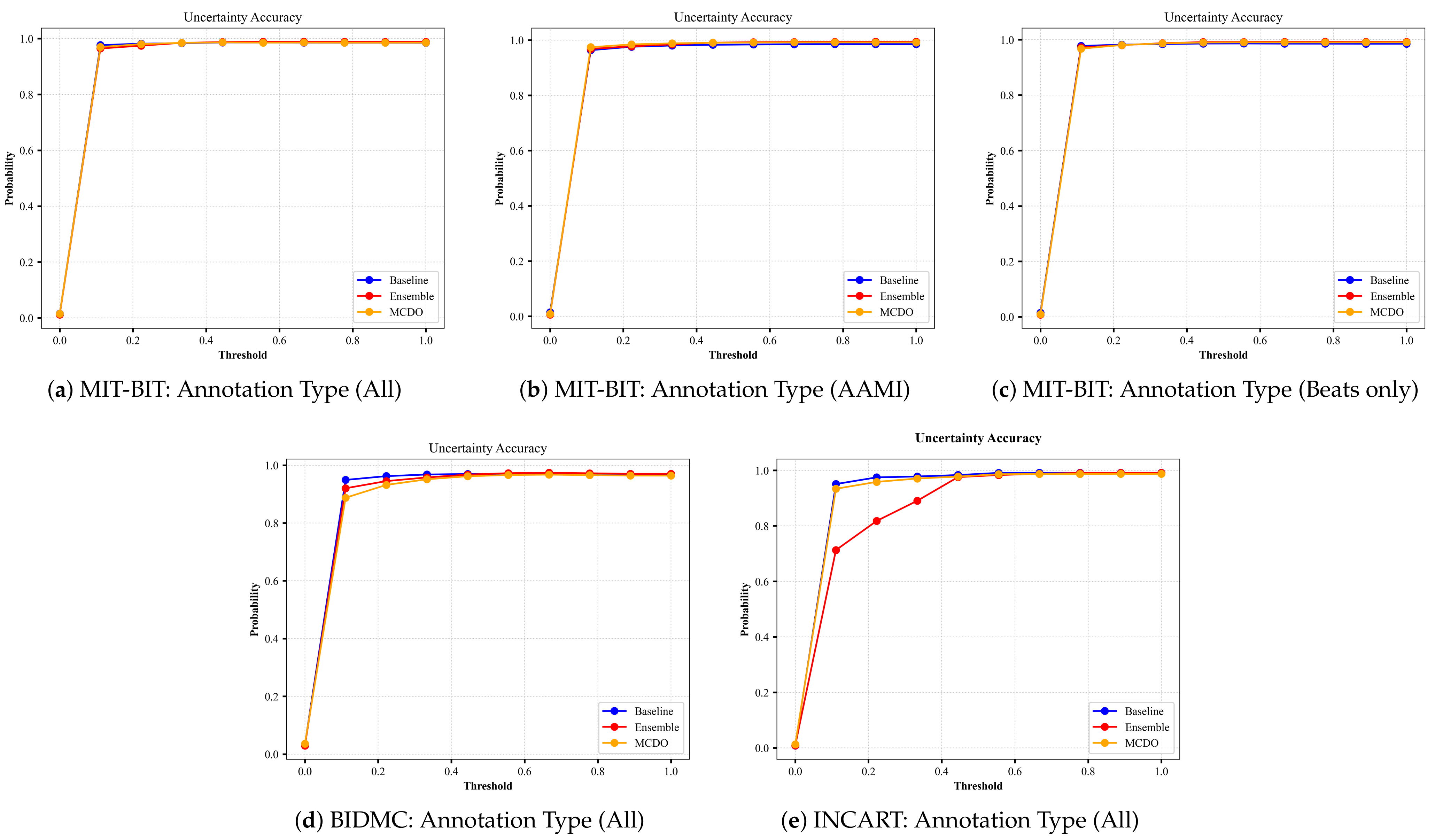
Similarly, we plot in Figure A5 the results of Equation (12) in which we measure the overall accuracy of the uncertainty estimation (AU) in each mode. We can observe that the uncertainty accuracy remains at a high rate close to 1 for varying thresholds of uncertainty, with a minor observation that the ensemble method in the INCART dataset shown in Equation (12) has a relatively low accuracy before the threshold value of 0.4.
5.3. Uncertainty Calibration
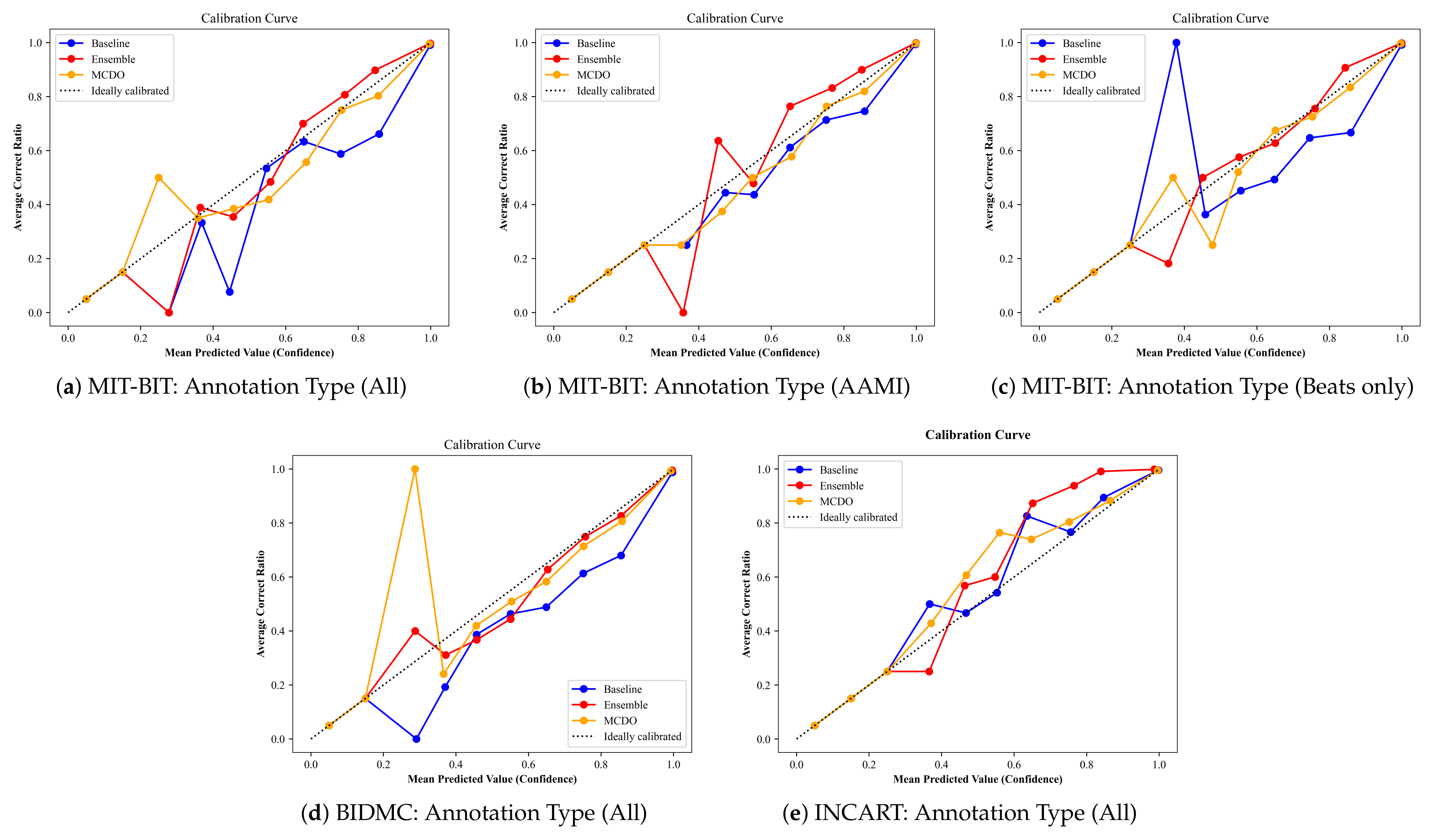
In addition to the metrics mentioned above, we apply an additional metric often called the model calibration, which is used to show the quality of uncertainty estimates in context to the overall performance. Figure A6 plots the average ratio of the correct predictions (i.e., when a model’s confidence in a prediction matches its probability of being correct) at each confidence interval for all input datasets. An ideal calibration would match the diagonal line from the bottom left to the top right. From these plots, we observe that the baseline method (i.e., softmax predictions) tends to be overconfident while MC-dropout (MCDO) produces almost well-calibrated estimations for higher confidence scores. In addition, it can be observed that all three methods tend to oscillate at low confidence scores, significantly below 0.5, but become more skillful as it moves toward the maximum confidence score. Notwithstanding, the estimated confidences by these methods cover the entire value range, which is very helpful for safety-critical applications.
6. Related Works
A successful ECG arrhythmia classification system should pass through three main phases: (1) preprocessing, (2) feature extraction, and (3) classification modeling. As with other types of signals, ECGs can be affected by many noise sources, and hence preprocessing phase ensures the readiness of input signals for further processing. Afterward, relevant features are extracted, especially raw signals, from the preprocessed signal using numerous techniques. This phase is so ever important as it highly impacts the performance of modeling methods. Accordingly, there have been quite some works on studying the effectiveness of employing various machine learning-based methods for electrocardiogram classification and recognition tasks. These studies are summarized in Table 4, including our work, and they are elaborated next.
The earliest work to construct a multi-class arrhythmic classification model was done by Ye et al. [50] using the general support vector machine (SVM) method, achieving 94.00% accuracy in classifying the MIT-BIH dataset into five categories using a specific feature engineering strategy that involves DWT coefficients with PCA and ICA. Zhang et al. [51] adapted the one-versus-one (OvO) feature ranking method, which focuses on the selection of effective subsets of features for distinguishing a class from others by making OvO comparisons. The extracted features are trained using the SVM method resulting in an average accuracy of 86.66%. Acharya et al. [53] developed a custom convolutional neural network to identify 5 heartbeats’ categories using a publicly available ECG dataset. By pre-processing the ECG signals into two sets; original (A) and noise-free (B) ECGs, they achieved in set A: accuracy 93.47%, sensitivity 96.01%, and TNR 91.64%, and in set B: accuracy 94.03%, sensitivity 96.71%, and TNR 91.54%. He et al. [54] introduced a lightweight CNN microarchitecture to diagnose 5 heartbeats’ arrhythmias categories that incur a lower computational cost and thus less communication across different processing units during distributed training. Their model attained an accuracy of 98.80% using ten-fold cross-validation method.
Furthermore, Jun et al. [55] proposed a preprocessing approach to transform ECG signals into 2D images and use the convolutional neural network (CNN) model as pattern recognition to classify a publicly available dataset of eight classes, achieving an accuracy of 99.05%, 97.85% sensitivity and 99.57% TNR. Rajpurkar et al. [52] took the task of heartbeat classification to an advanced level by introducing a custom arrhythmia ECG classification model using a specially made ECG dataset of a total of 14 classes. Their proposed model achieved a precision of 80.09% and a recall of 82.7%. Recently, Yang et al. [56] introduced a method that combines parametric and visual pattern features of ECG morphology for automatic diagnosis using a publicly available dataset of 15 classes, trained using KNN method, reporting an overall accuracy result 97.70%. Recently, Carvalho [57] slightly improved the results of Rajpurkar et al. using a public ECG dataset of 13 classes and achieved a precision of 84.8% and a recall of 82.2% while using a smaller neural network-based model than previously published methods with a goal to increase the performance while simultaneously keeping the neural networks short and fast. Finally, it is worth mentioning that some of the previous studies listed in Table 4 report their results using an improper metric, namely the accuracy, leading to inaccurate results, especially when using highly multi-class imbalanced datasets. On the contrary, this paper reports the classification results using a carefully selected set of metrics that accurately report the model performance in the existence of the input multi-class imbalanced datasets using the Precision, Recall, F1-score, and the area under the receiver operating characteristic curve (AUROC). These metrics have been traditionally known to assess the model’s performance accurately.
7. Conclusions
This paper presents an uncertainty-aware risk-aware deep learning-based predictive model design for accurate classification of cardiac arrhythmias successfully trained using three publicly available medical datasets and evaluated using a standard and task-specific set of metrics, providing more insights into the performance concerning safety-critical applications. Our experimental results achieve high-predicted diagnostic results compared with the existing models known to us. In addition, the results revealed that our classifier makes solid decisions with a higher level of confidence, marking predictions as correct when it is certain and incorrect when it is uncertain. Furthermore, we discovered that the MC-dropout method works well on our GRU-based model design operating in high certainty about its correct/incorrect predictions at varying uncertainty thresholds. Overall, we see strong potential by combining the two best-performing methods, i.e., deep ensembles and MC-dropout, with the strong capability of rejecting false examples with low confidence. For future works, we shall examine the effectiveness of the proposed method on the classification of other biomedical signal domains, particularly EEG signals, concerning the proposed uncertainty-oriented metrics. We shall also investigate the potential of applying other relevant groups of uncertainty quantification, namely fuzzy-based methods, to classify ECG signals and report our findings in the near future.
Funding
This research received no external funding.
Institutional Review Board Statement
Not applicable.
Informed Consent Statement
Not applicable.
Data Availability Statement
The data presented in this study are available on request from the corresponding author.
Acknowledgments
I want to thank Yahya Omar Asiri, MD (Physician fellow, King Fahad Medical City, Riyadh, Saudi Arabia) for the medical comments that significantly improved the manuscript.
Conflicts of Interest
The author declares no conflict of interest.
Appendix A
Figure A1.
Multiclass ROC curves of the input datasets using the Deep Ensemble method.
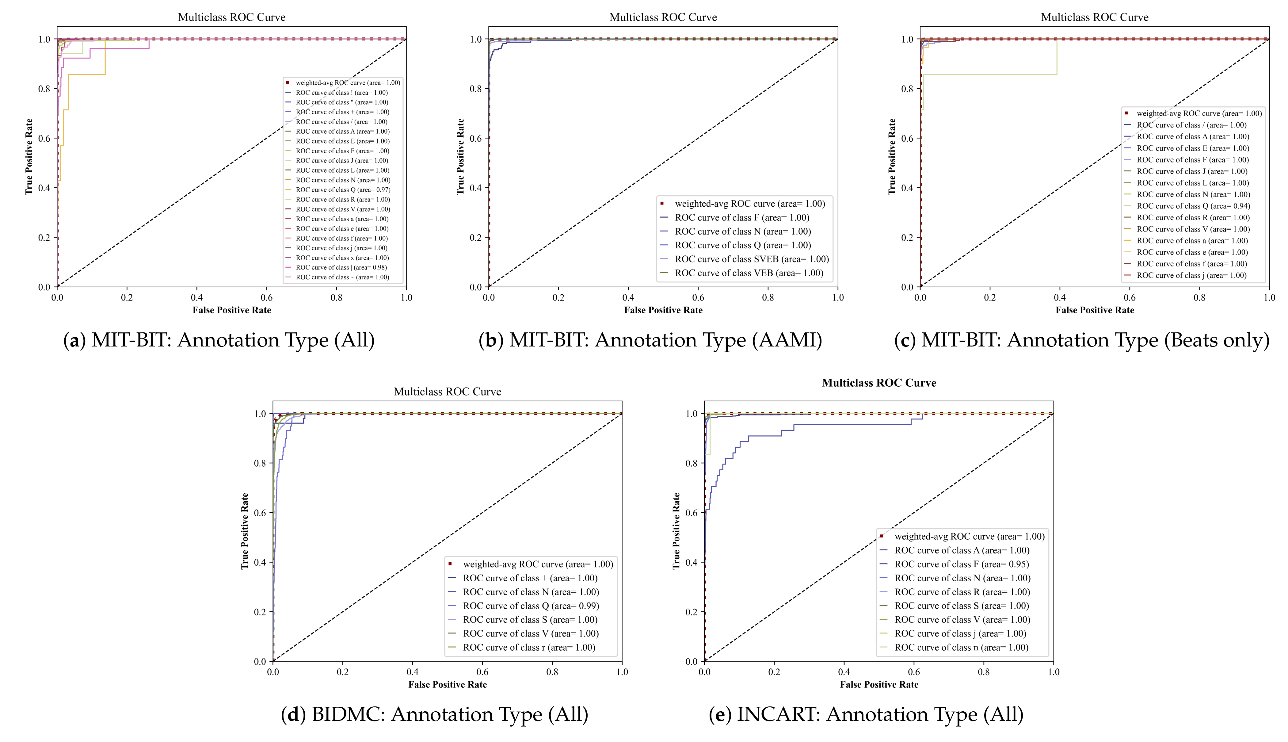
Figure A2.
Multiclass ROC curves using the Monte Carlo-based dropout method.
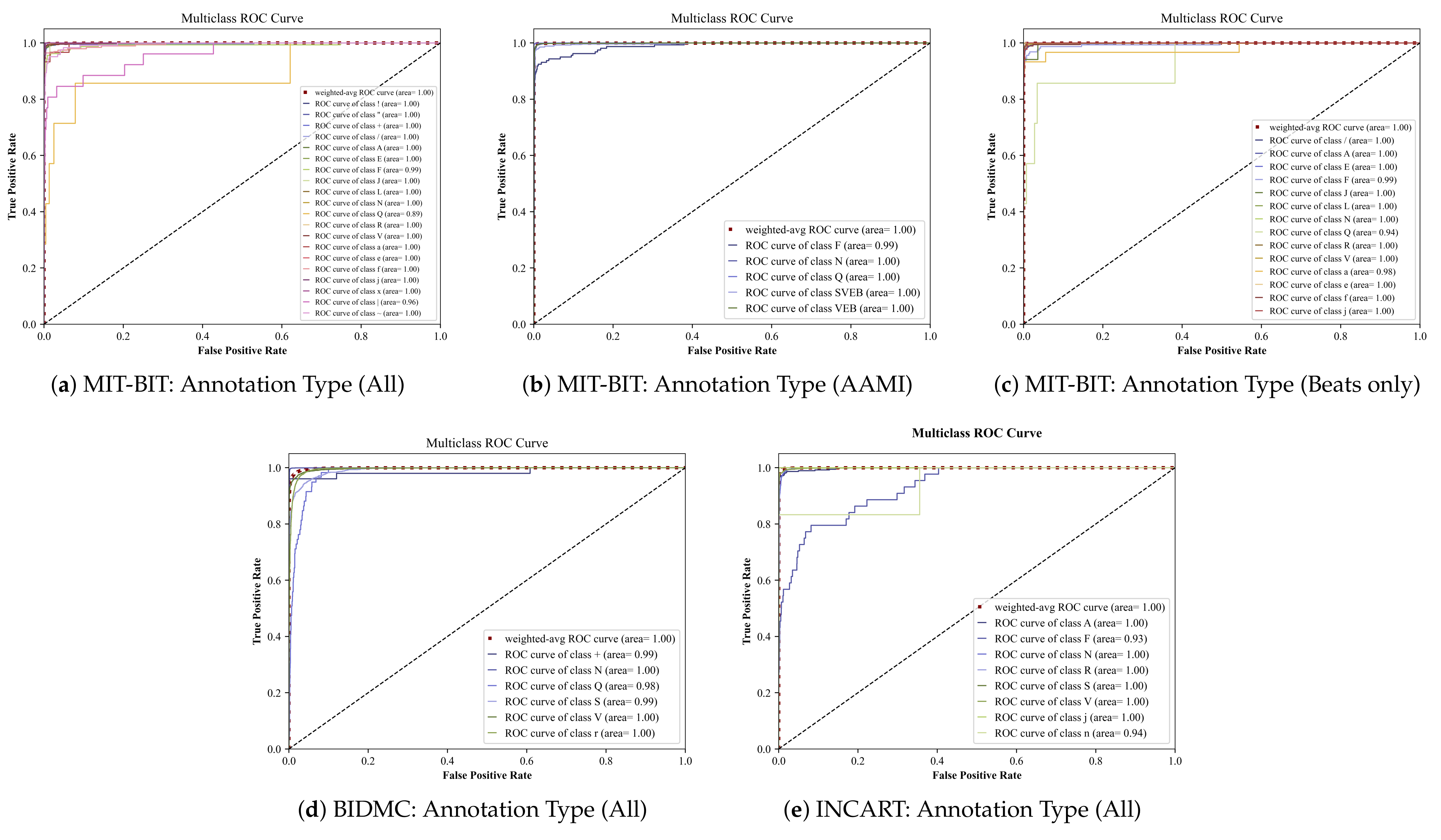
Figure A3.
The plots of from each input dataset for varying thresholds of uncertainty. The annotation type in each input dataset indicates the number of selected classes based on criteria explained in Section 3.1.
Figure A3.
The plots of from each input dataset for varying thresholds of uncertainty. The annotation type in each input dataset indicates the number of selected classes based on criteria explained in Section 3.1.
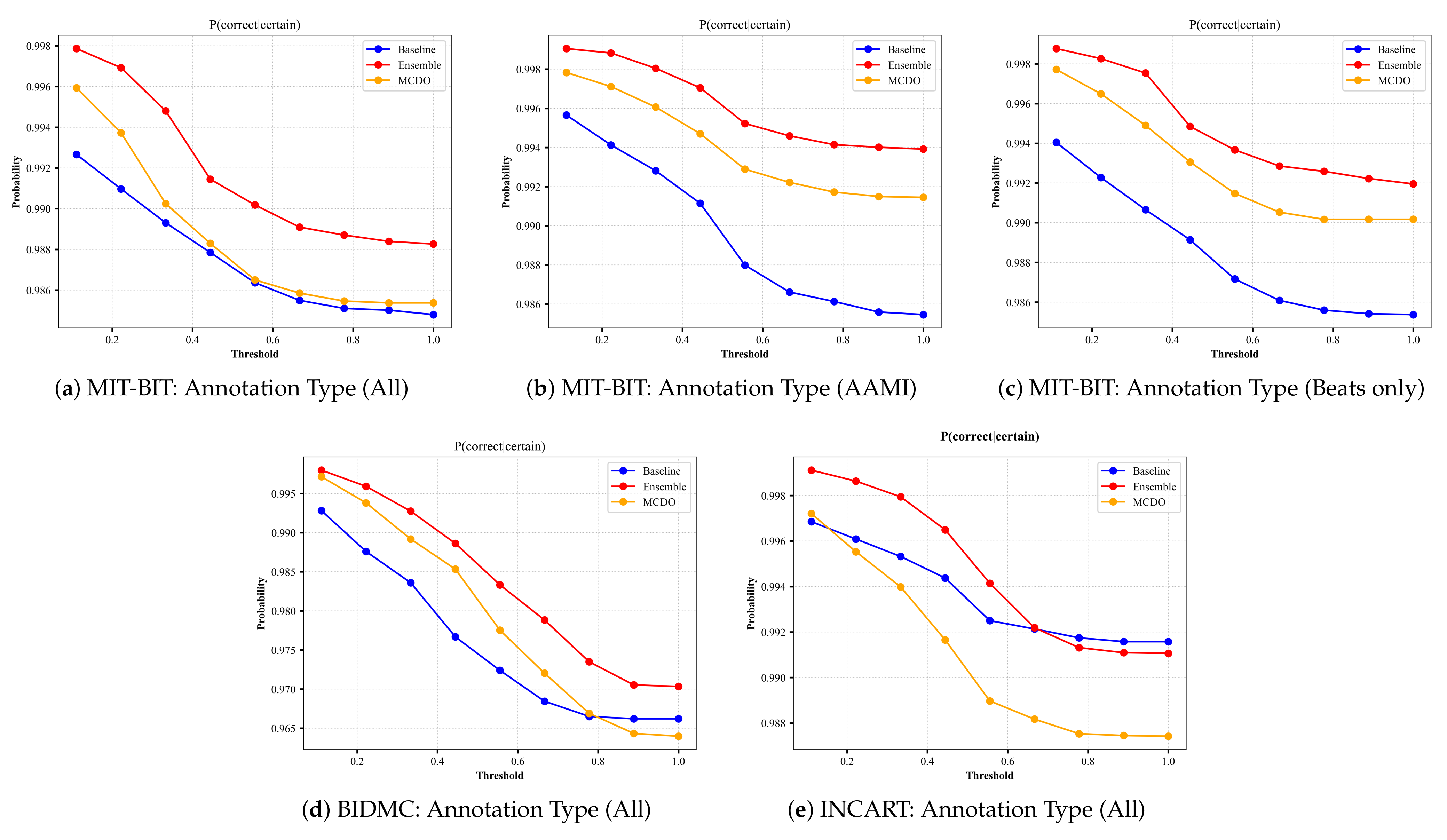
Figure A4.
The plots of from each input dataset for varying thresholds of uncertainty. The annotation type in each input dataset indicates the number of selected classes based on criteria explained in Section 3.1.
Figure A4.
The plots of from each input dataset for varying thresholds of uncertainty. The annotation type in each input dataset indicates the number of selected classes based on criteria explained in Section 3.1.
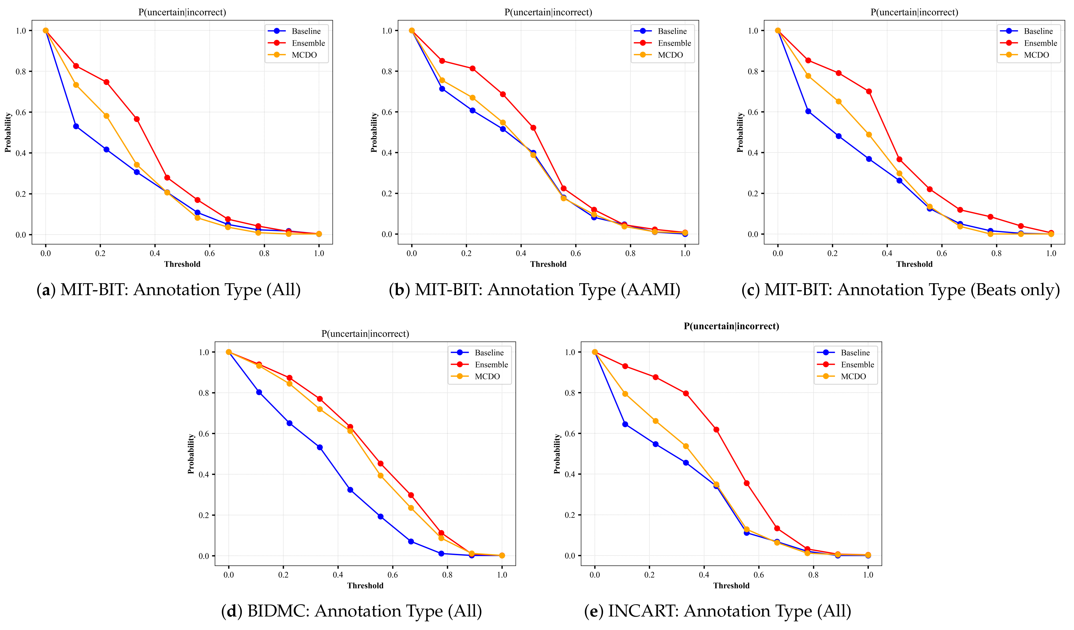
Figure A5.
The plots of Uncertainty Accuracy from each input dataset for varying thresholds of uncertainty. The annotation type in each input dataset indicates the number of selected classes based on criteria explained in Section 3.1.
Figure A5.
The plots of Uncertainty Accuracy from each input dataset for varying thresholds of uncertainty. The annotation type in each input dataset indicates the number of selected classes based on criteria explained in Section 3.1.

Figure A6.
The average ratio of the correct predictions at each confidence interval for all input datasets.
Figure A6.
The average ratio of the correct predictions at each confidence interval for all input datasets.

References
- Chang, K.C.; Hsieh, P.H.; Wu, M.Y.; Wang, Y.C.; Chen, J.Y.; Tsai, F.J.; Shih, E.S.; Hwang, M.J.; Huang, T.C. Usefulness of machine learning-based detection and classification of cardiac arrhythmias with 12-lead electrocardiograms. Can. J. Cardiol. 2021, 37, 94–104. [Google Scholar] [CrossRef]
- Hijazi, S.; Page, A.; Kantarci, B.; Soyata, T. Machine learning in cardiac health monitoring and decision support. Computer 2016, 49, 38–48. [Google Scholar] [CrossRef]
- Al-Zaiti, S.; Besomi, L.; Bouzid, Z.; Faramand, Z.; Frisch, S.; Martin-Gill, C.; Gregg, R.; Saba, S.; Callaway, C.; Sejdić, E. Machine learning-based prediction of acute coronary syndrome using only the pre-hospital 12-lead electrocardiogram. Nat. Commun. 2020, 11, 1–10. [Google Scholar]
- Giudicessi, J.R.; Schram, M.; Bos, J.M.; Galloway, C.D.; Shreibati, J.B.; Johnson, P.W.; Carter, R.E.; Disrud, L.W.; Kleiman, R.; Attia, Z.I.; et al. Artificial Intelligence–Enabled Assessment of the Heart Rate Corrected QT Interval Using a Mobile Electrocardiogram Device. Circulation 2021, 143, 1274–1286. [Google Scholar] [CrossRef]
- Kashou, A.H.; Noseworthy, P.A. Artificial Intelligence Capable of Detecting Left Ventricular Hypertrophy: Pushing the Limits of the Electrocardiogram? Europace 2020, 22, 338–339. [Google Scholar] [CrossRef]
- Kuncheva, L. Fuzzy Classifier Design; Springer Science & Business Media: Berlin/Heidelberg, Germany, 2000; Volume 49. [Google Scholar]
- Zhang, Y.; Zhou, Z.; Bai, H.; Liu, W.; Wang, L. Seizure classification from EEG signals using an online selective transfer TSK fuzzy classifier with joint distribution adaption and manifold regularization. Front. Neurosci. 2020, 14. [Google Scholar] [CrossRef]
- Postorino, M.N.; Versaci, M. A geometric fuzzy-based approach for airport clustering. Adv. Fuzzy Syst. 2014, 2014. [Google Scholar] [CrossRef] [Green Version]
- Neal, R.M. Bayesian Learning for Neural Networks; Springer Science & Business Media: Berlin/Heidelberg, Germany, 2012; Volume 118. [Google Scholar]
- Jospin, L.V.; Buntine, W.; Boussaid, F.; Laga, H.; Bennamoun, M. Hands-on Bayesian Neural Networks—A Tutorial for Deep Learning Users. arXiv 2020, arXiv:2007.06823. [Google Scholar]
- Gal, Y.; Ghahramani, Z. Dropout as a bayesian approximation: Representing model uncertainty in deep learning. In Proceedings of the International Conference on Machine Learning, PMLR, New York City, NY, USA, 20–22 June 2016; pp. 1050–1059. [Google Scholar]
- Hein, M.; Andriushchenko, M.; Bitterwolf, J. Why relu networks yield high-confidence predictions far away from the training data and how to mitigate the problem. In Proceedings of the IEEE/CVF Conference on Computer Vision and Pattern Recognition, Long Beach, CA, USA, 19–20 June 2019; pp. 41–50. [Google Scholar]
- Moon, J.; Kim, J.; Shin, Y.; Hwang, S. Confidence-aware learning for deep neural networks. In Proceedings of the International Conference on Machine Learning, PMLR, Virtual, 13–18 July 2020; pp. 7034–7044. [Google Scholar]
- Gacek, A. An Introduction to ECG Signal Processing and Analysis. In ECG Signal Processing, Classification and Interpretation: A Comprehensive Framework of Computational Intelligence; Gacek, A., Pedrycz, W., Eds.; Springer: London, UK, 2012; pp. 21–46. [Google Scholar] [CrossRef]
- Maglaveras, N.; Stamkopoulos, T.; Diamantaras, K.; Pappas, C.; Strintzis, M. ECG pattern recognition and classification using non-linear transformations and neural networks: A review. Int. J. Med. Inform. 1998, 52, 191–208. [Google Scholar] [CrossRef]
- Rai, H.M.; Trivedi, A.; Shukla, S. ECG signal processing for abnormalities detection using multi-resolution wavelet transform and Artificial Neural Network classifier. Measurement 2013, 46, 3238–3246. [Google Scholar] [CrossRef]
- Morita, H.; Kusano, K.F.; Miura, D.; Nagase, S.; Nakamura, K.; Morita, S.T.; Ohe, T.; Zipes, D.P.; Wu, J. Fragmented QRS as a marker of conduction abnormality and a predictor of prognosis of Brugada syndrome. Circulation 2008, 118, 1697. [Google Scholar] [CrossRef] [Green Version]
- Curtin, A.E.; Burns, K.V.; Bank, A.J.; Netoff, T.I. QRS complex detection and measurement algorithms for multichannel ECGs in cardiac resynchronization therapy patients. IEEE J. Transl. Eng. Health Med. 2018, 6, 1–11. [Google Scholar] [CrossRef]
- Li, C.; Zheng, C.; Tai, C. Detection of ECG characteristic points using wavelet transforms. IEEE Trans. Biomed. Eng. 1995, 42, 21–28. [Google Scholar] [PubMed]
- Chung, J.; Gulcehre, C.; Cho, K.; Bengio, Y. Gated Feedback Recurrent Neural Networks. In Proceedings of the 32nd International Conference on Machine Learning, Lille, France, 6–11 July 2015; Bach, F., Blei, D., Eds.; PMLR: Lille, France, 2015; Volume 37, pp. 2067–2075. [Google Scholar]
- Xia, Y.; Xiang, M.; Li, Z.; Mandic, D.P. Chapter 12-Echo State Networks for Multidimensional Data: Exploiting Noncircularity and Widely Linear Models. In Adaptive Learning Methods for Nonlinear System Modeling; Comminiello, D., Principe, J.C., Eds.; Butterworth-Heinemann: Oxford, UK, 2018; pp. 267–288. [Google Scholar] [CrossRef]
- Olah, C. Understanding LSTM Networks. Available online: https://colah.github.io/posts/2015-08-Understanding-LSTMs/ (accessed on 17 June 2021).
- Chung, J.; Gulcehre, C.; Cho, K.; Bengio, Y. Empirical evaluation of gated recurrent neural networks on sequence modeling. arXiv 2014, arXiv:1412.3555. [Google Scholar]
- Hochreiter, S.; Schmidhuber, J. Long short-term memory. Neural Comput. 1997, 9, 1735–1780. [Google Scholar] [CrossRef] [PubMed]
- Gers, F.A.; Schraudolph, N.N.; Schmidhuber, J. Learning precise timing with LSTM recurrent networks. J. Mach. Learn. Res. 2002, 3, 115–143. [Google Scholar]
- Cho, K.; Van Merrinboer, B.; Bahdanau, D.; Bengio, Y. On the properties of neural machine translation: Encoder-decoder approaches. arXiv 2014, arXiv:1409.1259. [Google Scholar]
- Graves, A. Practical variational inference for neural networks. In Proceedings of the Advances in Neural Information Processing Systems, Granada, Spain, 12–15 December 2011; pp. 2348–2356. [Google Scholar]
- Kendall, A.; Gal, Y. What uncertainties do we need in bayesian deep learning for computer vision? arXiv 2017, arXiv:1703.04977. [Google Scholar]
- Welling, M.; Teh, Y.W. Bayesian learning via stochastic gradient Langevin dynamics. In Proceedings of the 28th international conference on machine learning (ICML-11), Citeseer, Bellevue, WA, USA, 28 June–2 July 2011; pp. 681–688. [Google Scholar]
- Hernández-Lobato, J.M.; Adams, R. Probabilistic backpropagation for scalable learning of bayesian neural networks. In Proceedings of the International Conference on Machine Learning, PMLR, Lille, France, 7–9 July 2015; pp. 1861–1869. [Google Scholar]
- Blundell, C.; Cornebise, J.; Kavukcuoglu, K.; Wierstra, D. Weight uncertainty in neural network. In Proceedings of the International Conference on Machine Learning, PMLR, Lille, France, 7–9 July 2015; pp. 1613–1622. [Google Scholar]
- Goldberger, A.; Amaral, L.; Glass, L.; Hausdorff, J.; Ivanov, P.C.; Mark, R.; Mietus, J.; Moody, G.; Peng, C.; Stanley, H. PhysioBank, PhysioToolkit, and PhysioNet: Components of a new research resource for complex physiologic signals. Circulation 2000, 101, E215–E220. [Google Scholar] [CrossRef] [PubMed] [Green Version]
- Moody, G.B.; Mark, R.G. The impact of the MIT-BIH arrhythmia database. IEEE Eng. Med. Biol. Mag. 2001, 20, 45–50. [Google Scholar] [CrossRef]
- Baim, D.S.; Colucci, W.S.; Monrad, E.S.; Smith, H.S.; Wright, R.F.; Lanoue, A.; Gauthier, D.F.; Ransil, B.J.; Grossman, W.; Braunwald, E. Survival of patients with severe congestive heart failure treated with oral milrinone. J. Am. Coll. Cardiol. 1986, 7, 661–670. [Google Scholar] [CrossRef] [Green Version]
- Research Resource for Complex Physiologic Signals. Available online: https://physionet.org/ (accessed on 17 June 2021).
- Association for the Advancement of Medical Instrumentation. Testing and Reporting Performance Results of Cardiac Rhythm and ST Segment Measurement Algorithms; Association for the Advancement of Medical Instrumentation: Arlington, VA, USA, 1998. [Google Scholar]
- Bleeker, G.B.; Schalij, M.J.; Molhoek, S.G.; Verwey, H.F.; Holman, E.R.; Boersma, E.; Steendijk, P.; Van Der Wall, E.E.; Bax, J.J. Relationship between QRS duration and left ventricular dyssynchrony in patients with end-stage heart failure. J. Cardiovasc. Electrophysiol. 2004, 15, 544–549. [Google Scholar] [CrossRef]
- Sipahi, I.; Carrigan, T.P.; Rowland, D.Y.; Stambler, B.S.; Fang, J.C. Impact of QRS duration on clinical event reduction with cardiac resynchronization therapy: Meta-analysis of randomized controlled trials. Arch. Intern. Med. 2011, 171, 1454–1462. [Google Scholar] [CrossRef] [PubMed] [Green Version]
- Lakshminarayanan, B.; Pritzel, A.; Blundell, C. Simple and scalable predictive uncertainty estimation using deep ensembles. arXiv 2016, arXiv:1612.01474. [Google Scholar]
- Leibig, C.; Allken, V.; Ayhan, M.S.; Berens, P.; Wahl, S. Leveraging uncertainty information from deep neural networks for disease detection. Sci. Rep. 2017, 7, 1–14. [Google Scholar] [CrossRef] [Green Version]
- Gal, Y.; Ghahramani, Z. Dropout as a Bayesian approximation: Appendix. arXiv 2015, arXiv:1506.02157. [Google Scholar]
- Abadi, M.; Agarwal, A.; Barham, P.; Brevdo, E.; Chen, Z.; Citro, C.; Corrado, G.S.; Davis, A.; Dean, J.; Devin, M.; et al. TensorFlow: Large-Scale Machine Learning on Heterogeneous Systems. 2015. Available online: tensorflow.org (accessed on 17 June 2021).
- Team, K. Simple. Flexible. Powerful. Available online: https://www.myob.com/nz/about/news/2020/simple–flexible–powerful—the-new-myob-essentials (accessed on 17 June 2021).
- Kingma, D.; Ba, J. Adam: A method for stochastic optimization. arXiv 2014, arXiv:1412.6980. [Google Scholar]
- Aseeri, A. Noise-Resilient Neural Network-Based Adversarial Attack Modeling for XOR Physical Unclonable Functions. J. Cyber Secur. Mobil. 2020, 331–354. [Google Scholar] [CrossRef]
- Sokolova, M.; Lapalme, G. A systematic analysis of performance measures for classification tasks. Inf. Process. Manag. 2009, 45, 427–437. [Google Scholar] [CrossRef]
- Henne, M.; Schwaiger, A.; Roscher, K.; Weiss, G. Benchmarking Uncertainty Estimation Methods for Deep Learning With Safety-Related Metrics. Available online: http://ceur-ws.org/Vol-2560/paper35.pdf (accessed on 17 June 2021).
- Mukhoti, J.; Gal, Y. Evaluating bayesian deep learning methods for semantic segmentation. arXiv 2018, arXiv:1811.12709. [Google Scholar]
- Lemaître, G.; Nogueira, F.; Aridas, C.K. Imbalanced-learn: A Python Toolbox to Tackle the Curse of Imbalanced Datasets in Machine Learning. J. Mach. Learn. Res. 2017, 18, 1–5. [Google Scholar]
- Ye, C.; Kumar, B.V.; Coimbra, M.T. Combining general multi-class and specific two-class classifiers for improved customized ECG heartbeat classification. In Proceedings of the 21st International Conference on Pattern Recognition (ICPR2012), Tsukuba, Japan, 11–15 November 2012; pp. 2428–2431. [Google Scholar]
- Zhang, Z.; Dong, J.; Luo, X.; Choi, K.S.; Wu, X. Heartbeat classification using disease-specific feature selection. Comput. Biol. Med. 2014, 46, 79–89. [Google Scholar] [CrossRef]
- Rajpurkar, P.; Hannun, A.Y.; Haghpanahi, M.; Bourn, C.; Ng, A.Y. Cardiologist-level arrhythmia detection with convolutional neural networks. arXiv 2017, arXiv:1707.01836. [Google Scholar]
- Acharya, U.R.; Oh, S.L.; Hagiwara, Y.; Tan, J.H.; Adam, M.; Gertych, A.; San Tan, R. A deep convolutional neural network model to classify heartbeats. Comput. Biol. Med. 2017, 89, 389–396. [Google Scholar] [CrossRef]
- He, Z.; Zhang, X.; Cao, Y.; Liu, Z.; Zhang, B.; Wang, X. LiteNet: Lightweight neural network for detecting arrhythmias at resource-constrained mobile devices. Sensors 2018, 18, 1229. [Google Scholar] [CrossRef] [Green Version]
- Jun, T.J.; Nguyen, H.M.; Kang, D.; Kim, D.; Kim, D.; Kim, Y.H. ECG arrhythmia classification using a 2-D convolutional neural network. arXiv 2018, arXiv:1804.06812. [Google Scholar]
- Yang, H.; Wei, Z. Arrhythmia recognition and classification using combined parametric and visual pattern features of ECG morphology. IEEE Access 2020, 8, 47103–47117. [Google Scholar] [CrossRef]
- Carvalho, C.S. A deep-learning classifier for cardiac arrhythmias. arXiv 2020, arXiv:2011.05471. [Google Scholar]
Figure 1.
An electrocardiogram signal waveform.

Figure 2.
Illustration the difference between of (a) Long Short-Term Memory (LSTM) and (b) Gated Recurrent Unit (GRU).
Figure 2.
Illustration the difference between of (a) Long Short-Term Memory (LSTM) and (b) Gated Recurrent Unit (GRU).

Figure 3.
Moving window-based segmentation approach.
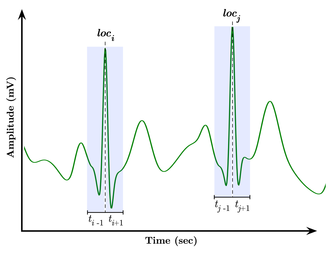
Figure 4.
The processing pipeline for the cardiac arrhythmia classification system.

Figure 5.
The GRU-based model architecture design. The number of GRU units is stated between parenthesis. Similarly, the dropout value of each dropout layer is stated between parenthesis.
Figure 5.
The GRU-based model architecture design. The number of GRU units is stated between parenthesis. Similarly, the dropout value of each dropout layer is stated between parenthesis.


Table 1.
Distribution of heartbeat annotation codes used by the selected databases in this paper.
| (a) The number of annotations used by each database (blue colored codes indicate beats-only annotations) | |||||||||||||||||||||||||||
| Database | Records | Annotation Codes Used by the Database | Total | ||||||||||||||||||||||||
| N | A | V | ∼ | | | Q | / | f | + | x | F | j | L | a | J | n | R | [ | ! | ] | E | " | e | r | S | |||
| MIT-BIH | 48 | 74,965 | 2545 | 7126 | 614 | 132 | 33 | 7018 | 982 | 1243 | 193 | 802 | 229 | 8066 | 150 | 83 | 0 | 7251 | 6 | 472 | 6 | 106 | 437 | 16 | 0 | 2 | 112,477 |
| INCART | 75 | 150,253 | 1942 | 19,995 | 0 | 0 | 0 | 0 | 0 | 0 | 0 | 219 | 92 | 0 | 0 | 0 | 32 | 3171 | 0 | 0 | 0 | 0 | 0 | 0 | 0 | 16 | 175,720 |
| BIDMC | 15 | 1,578,105 | 0 | 28,165 | 0 | 0 | 293 | 0 | 0 | 258 | 0 | 0 | 0 | 0 | 0 | 0 | 0 | 0 | 0 | 0 | 0 | 5 | 0 | 0 | 10,353 | 5314 | 1,622,493 |
| (b) AAMI classes vs. MIT-BIH labels | |||||||||||||||||||||||||||
| AAMI Class | MIT-BIH Beat Annotations | Number of Heartbeats | |||||||||||||||||||||||||
| N | N, L, R, e, j | 90,527 | |||||||||||||||||||||||||
| SVEB | A, a, J, S | 2780 | |||||||||||||||||||||||||
| VEB | V, E | 7232 | |||||||||||||||||||||||||
| Q | P or /, f, Q | 8033 | |||||||||||||||||||||||||
| F | F | 802 | |||||||||||||||||||||||||
| Total | 109,374 | ||||||||||||||||||||||||||
Table 2.
Classification results of five-sampling deep ensemble method using the three input cardiac arrhythmias datasets for a different set of annotations, where precision, recall, F1-score are the mean precision, mean recall, and the mean F1-score overall classes, weighted by the size of each class. The annotation type in each input dataset indicates the number of selected classes based on criteria explained in Section 3.1.
| Dataset | Annotation Type (Size) | Evaluation Metric | |||
|---|---|---|---|---|---|
| Precision | Recall | F1-Score | AUROC | ||
| MIT-BIT | All (20 classes) | 0.9894 | 0.9882 | 0.9887 | 0.9972 |
| Beats only (14 classes) | 0.9921 | 0.9919 | 0.9920 | 0.9955 | |
| AAMI (5 classes) | 0.9939 | 0.9939 | 0.9939 | 0.9987 | |
| BIDMC | All (6 classes) | 0.9756 | 0.9703 | 0.9725 | 0.9960 |
| INCART | All (8 classes) | 0.9940 | 0.9910 | 0.9923 | 0.9922 |
Table 3.
Classification results of 50-iter Monte Carlo-based dropout method using the three input cardiac arrhythmias datasets for a different set of annotations, where precision, recall, F1-score are the mean precision, mean recall, and the mean F1-score overall classes, weighted by the size of each class. The annotation type in each input dataset indicates the number of selected classes based on criteria explained in Section 3.1.
| Dataset | Annotation Type (Size) | Evaluation Metric | |||
|---|---|---|---|---|---|
| Precision | Recall | F1-Score | AUROC | ||
| MIT-BIT | All (20 classes) | 0.9874 | 0.9853 | 0.9862 | 0.9914 |
| Beats only (14 classes) | 0.9908 | 0.9902 | 0.9904 | 0.9932 | |
| AAMI (5 classes) | 0.9917 | 0.9914 | 0.9915 | 0.9970 | |
| BIDMC | All (6 classes) | 0.9718 | 0.9639 | 0.9673 | 0.9925 |
| INCART | All (8 classes) | 0.9921 | 0.9874 | 0.9894 | 0.9834 |
Table 4.
List of previous efforts in ECG classification compared to the paper’s results.
| Authors | Year of Publish | Dataset | Number of Classes | Model Performance |
|---|---|---|---|---|
| Ye et al. [50] | 2012 | MIT-BIH | 5 | Acc: 94% |
| Zhang et al. [51] | 2014 | MIT-BIH | 4 | Acc: 86.66% |
| Rajpurkar et al. [52] | 2017 | Private dataset | 14 | Precision: 80.09% Recall: 82.7% |
| Acharya et al. [53] | 2017 | MIT-BIH | 5 | Noisy set: Acc: 93.47% Sen: 96.01% TNR: 91.64% Noise-free set: Acc: 94.03% Sen: 96.71% TNR: 91.54% |
| He et al. [54] | 2018 | MIT-BIH | 5 | Acc: 98.80% |
| Jun et al. [55] | 2018 | MIT-BIH | 8 | Acc: 99.05% Sen: 99.85% TNR: 99.57% |
| Yang et al. [56] | 2020 | MIT-BIH | 15 | Acc: 97.70% |
| Carvalho [57] | 2020 | MIT-BIH | 13 | Precision: 84.8% Recall: 82.2% |
| This study | 2021 | MIT-BIH | 20 | DE mode: Precision: 98.94% Recall: 98.82% F1: 98.87% MCDO mode: Precision: 98.74% Recall: 98.53% F1: 98.62% |
| BIDMC | 6 | DE mode: Precision: 97.57% Recall: 97.03% F1: 97.25% MCDO mode: Precision: 97.18% Recall: 97.39% F1: 96.73% | ||
| INCART | 8 | DE mode: Precision: 99.4% Recall: 99.1% F1: 99.23% MCDO mode: Precision: 99.21% Recall: 98.74% F1: 96.94% |
Publisher’s Note: MDPI stays neutral with regard to jurisdictional claims in published maps and institutional affiliations. |
© 2021 by the author. Licensee MDPI, Basel, Switzerland. This article is an open access article distributed under the terms and conditions of the Creative Commons Attribution (CC BY) license (https://creativecommons.org/licenses/by/4.0/).
Share and Cite
MDPI and ACS Style
Aseeri, A.O. Uncertainty-Aware Deep Learning-Based Cardiac Arrhythmias Classification Model of Electrocardiogram Signals. Computers 2021, 10, 82. https://0-doi-org.brum.beds.ac.uk/10.3390/computers10060082
AMA Style
Aseeri AO. Uncertainty-Aware Deep Learning-Based Cardiac Arrhythmias Classification Model of Electrocardiogram Signals. Computers. 2021; 10(6):82. https://0-doi-org.brum.beds.ac.uk/10.3390/computers10060082
Chicago/Turabian StyleAseeri, Ahmad O. 2021. "Uncertainty-Aware Deep Learning-Based Cardiac Arrhythmias Classification Model of Electrocardiogram Signals" Computers 10, no. 6: 82. https://0-doi-org.brum.beds.ac.uk/10.3390/computers10060082
Note that from the first issue of 2016, this journal uses article numbers instead of page numbers. See further details here.