
A Comparative Analysis of Semi-Supervised Learning in Detecting Burst Header Packet Flooding Attack in Optical Burst Switching Network


Abstract
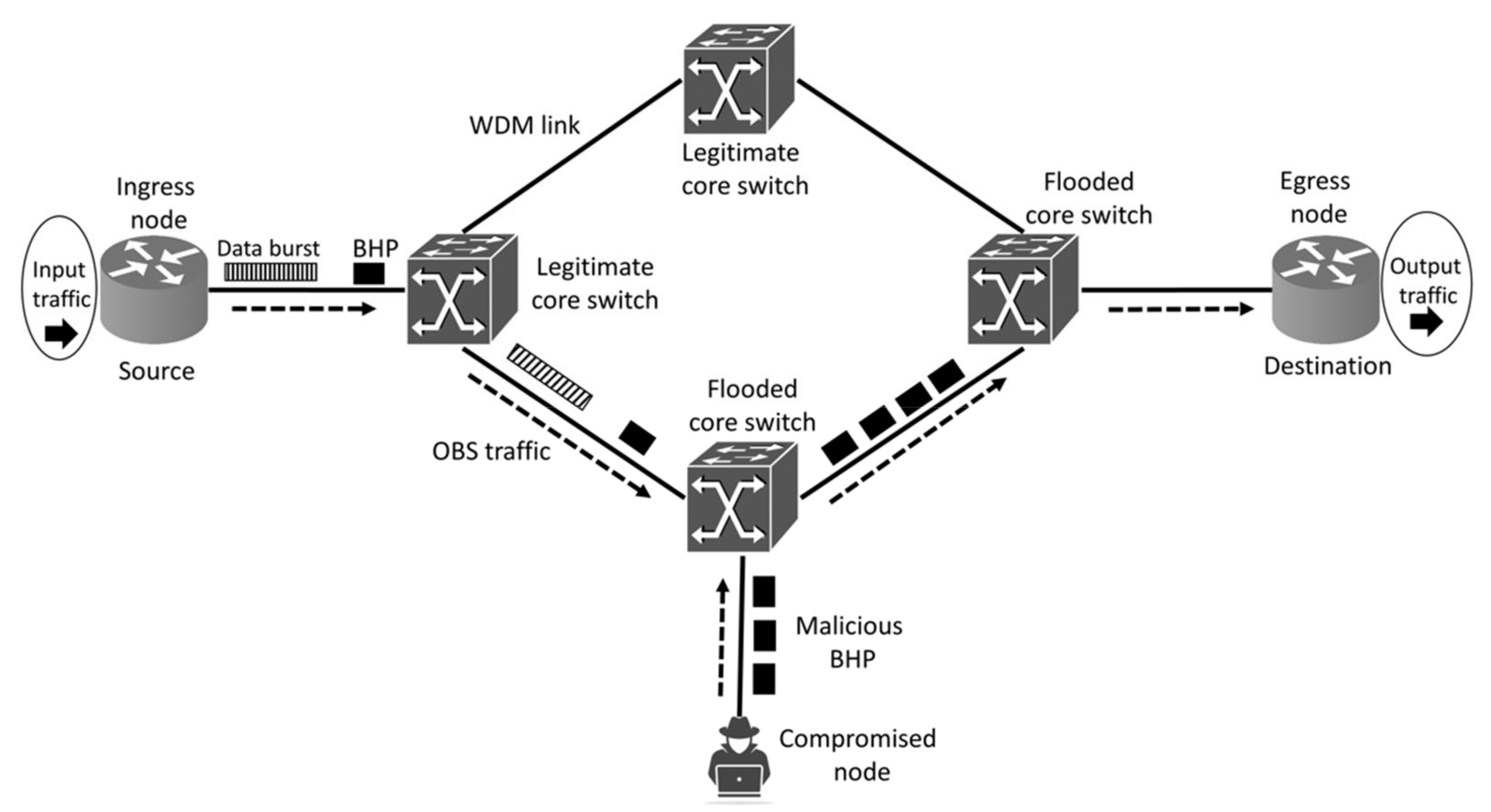
:1. Introduction
- This paper presents a comparative study of the existing works on semi-supervised machine learning (SSML) based BHP flooding attack detection in OBS network. The outcome of this study will help the research community to better understand the SSML-based models for optical burst switching network related vulnerabilities.
- This study found that the SSML-based approaches outperformed the supervised learning-based approaches when a smaller sized labeled data is available to train the classification models.
2. Literature Review
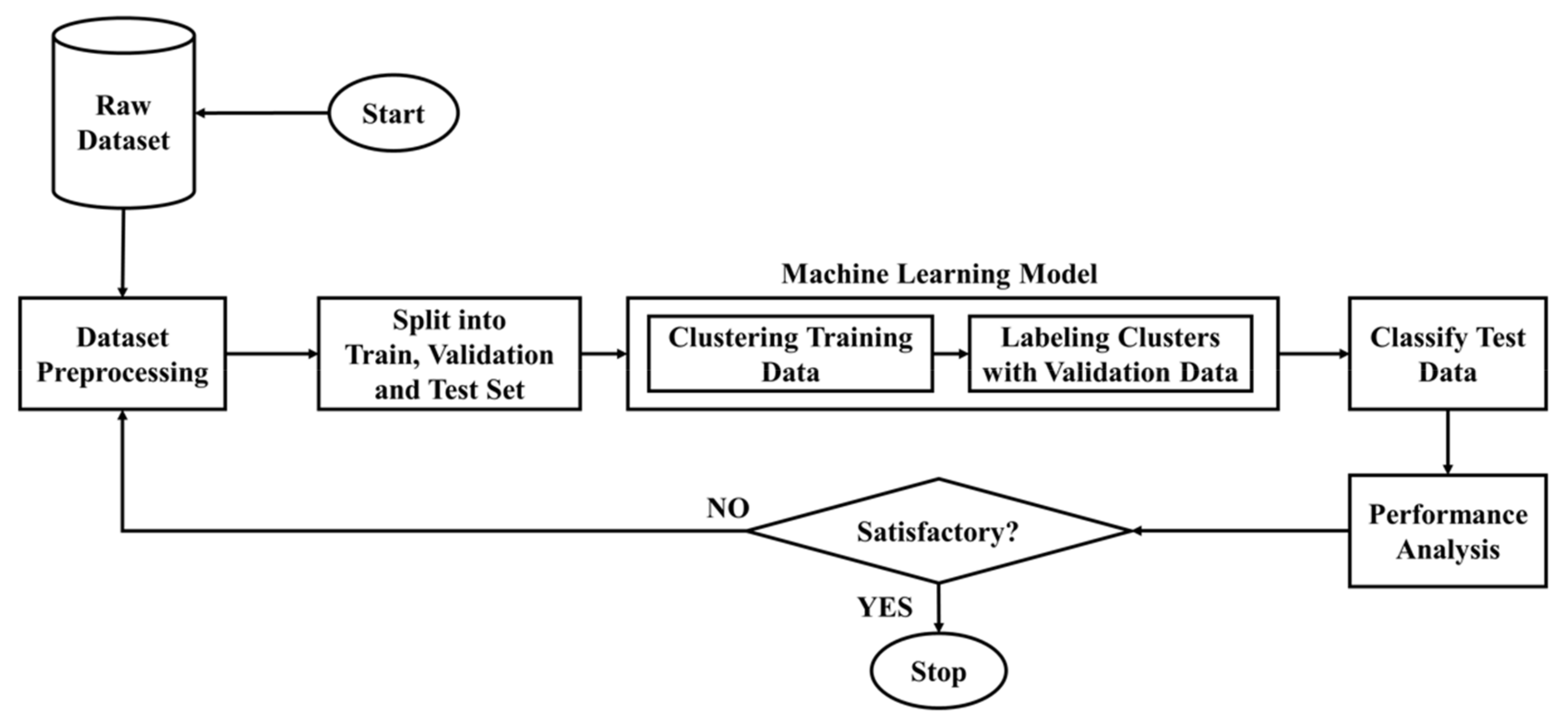
3. Materials and Methods
3.1. Study 1: SSML with K-Means Clustering
| Algorithm 1 k-Means Algorithm [19] | |
| Input: data point for dataset X, i.e. (x є X) and number of centers k | |
| 1. | Select an initial partition with k clusters |
| 2. | Repeat |
| 3. | Compute a new partition by assigning each data point to its nearest cluster center |
| 4. | Generate new cluster centers |
| 5. | Until cluster membership become stable |
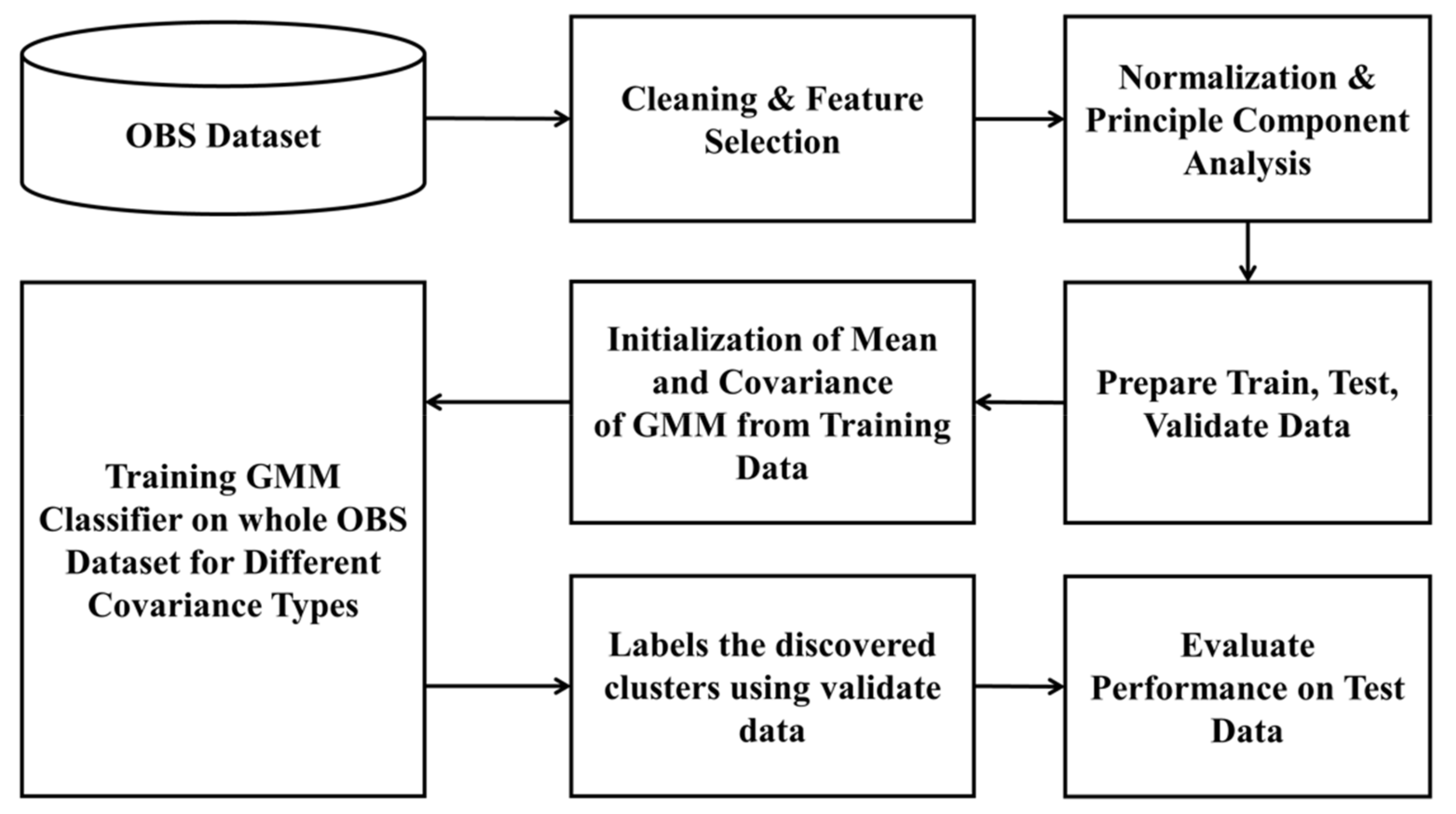
3.2. Study 2: SSML with Gaussian Mixture Model (GMM) Clustering
| Algorithm 2 EM Algorithm for Mixture of Gaussians | |
| 1. | Given: All points xєX that are mixtures of K Gaussians |
| 2. | Goal: Find π1,…, πk and Θ1,…, Θk such that is maximized |
| 3. | Initialize the means μk, variances Σk for each component |
| 4. | Initialize the mixing coefficients π and evaluate the initial value of log likelihood L(Θ) |
| 5. | Expectation step: Evaluate weights wik |
| 6. | Maximization step: Re-evaluate parameters , and |
| 7. | Evaluate L(Θnew) |
| 8. | ifL(Θnew) converged then stop |
| 9. | else goto 4 |
| 10. | end if |
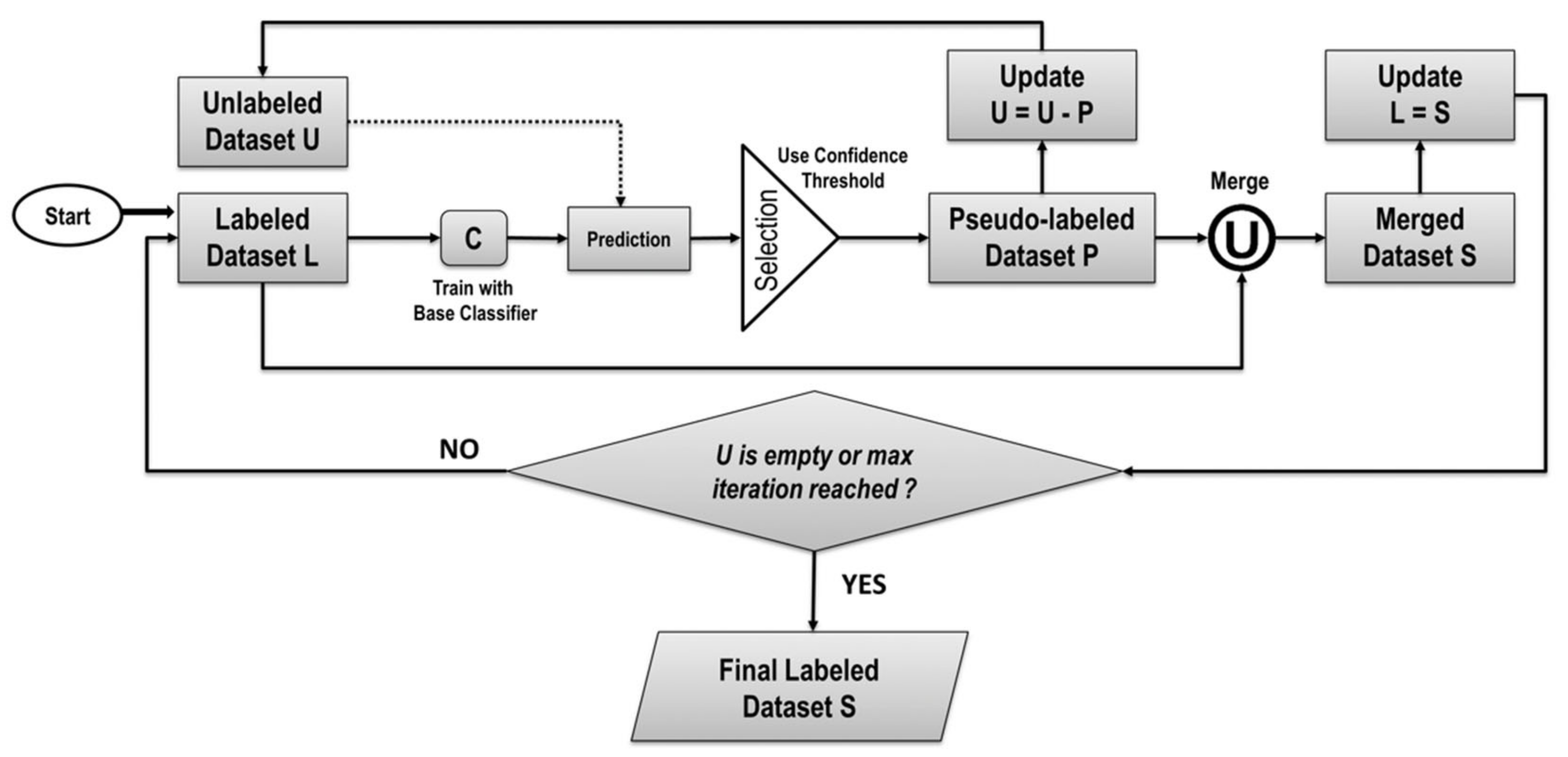
3.3. Study 3: SSML with Self-Training
| Algorithm 3 Classical Self-Training Algorithm (ST) [17] | |
| 1. | N: Iteration counter = 1; C: Base classifier, L: Labeled data, U: Unlabeled data, maxCount: number of iterations allowed, H: Confidence Threshold |
| 2. | while (U! = empty) and (N < maxCount) do |
| 3. | Train C on L |
| 4. | for eachdiinUdo |
| 5. | Assign pseudo-label to di based on prediction confidence |
| 6. | end for |
| 7. | Select a set P of the high-confidence predictions from U based on threshold H |
| 8. | Update N = N + 1; U = U - P; L = L U P |
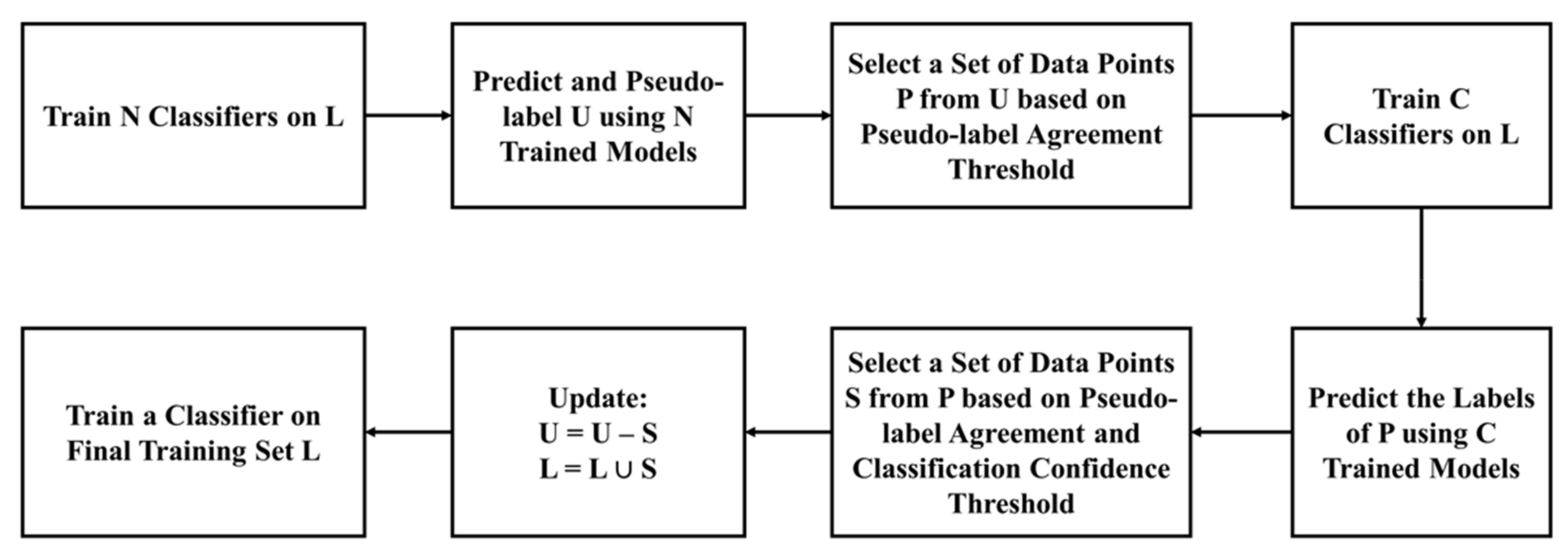
3.4. Study 4: SSML with Modified Self-Training
| Algorithm 4 Modified Self-Training Algorithm (MST) [5] | |
| 1. | C1: A set of N classifiers, C2: A set of M classifiers, F: Final classifier, L: Labeled data, U: Unlabeled data, K: Set of empty datasets, P, S: Empty dataset, V1: 1st stage pseudo-label agreement threshold, V2: 2nd stage pseudo-label agreement threshold, H: Classification confidence threshold |
| 2. | C1= {C11,C12,..C1N}, C2= {C21,C22,...C2M}, i = 1, K= {K1,K2,...KN} |
| 3. | for eachcinC1do |
| 4. | Train c by training set L |
| 5. | for each d in Udo |
| 6. | Assign pseudo-label to d based on prediction confidence |
| 7. | Save d along with the pseudo-label in set Ki |
| 8. | end for |
| 9. | i = i + 1 |
| 10. | end for |
| 11. | for eachdinUdo |
| 12. | compute pseudo-label agreement (votes) for d in K |
| 13. | if votes >= V1 then |
| 14. | copy d and save in set P |
| 15. | end if |
| 16. | end for |
| 17. | i = 1 and K1,K2,...KN = {} |
| 18. | for eachcinC2do |
| 19. | Train c by training set L |
| 20. | for each d in P do |
| 21. | Classify d by model c |
| 22. | if classification confidence >= H then |
| 23. | Save d along with the pseudo-label in set Ki |
| 24. | end if |
| 25. | end for |
| 26. | i = i + 1; |
| 27. | end for |
| 28. | for eachdinPdo |
| 29. | compute pseudo-label agreement(votes) for d in K |
| 30. | if votes >= V2 then |
| 31. | copy d in set S |
| 32. | end if |
| 33. | end for |
| 34. | Update U by removing S from U: U = U - S |
| 35. | Update L by joining S with L: L = L U S |
| 36. | Train classifier F by training set L |
| 37. | Classify U by F and predict labels for all the points in U |
| 38. | Output: Fully labeled dataset |
4. Experiment and Analyses
4.1. Experimental and Environmental Setup
- First Case: we trained SSML models to classify the nodes (i.e., data instances) in the dataset into two distinct classes: Behaving (B) and Not Behaving (NB) based on the target attribute ‘Node Status’.
- Second Case: models were trained to classify the nodes into three distinct classes: Behaving (B), Not Behaving (NB) and Potentially Not Behaving (PNB) based on the target attribute ‘Node Status’.
- Third Case: models were trained to classify the nodes into four distinct classes based on the target attribute ‘Class’, which has four distinct class values: No-Block, Block, NB- wait, and NB-No-Block.
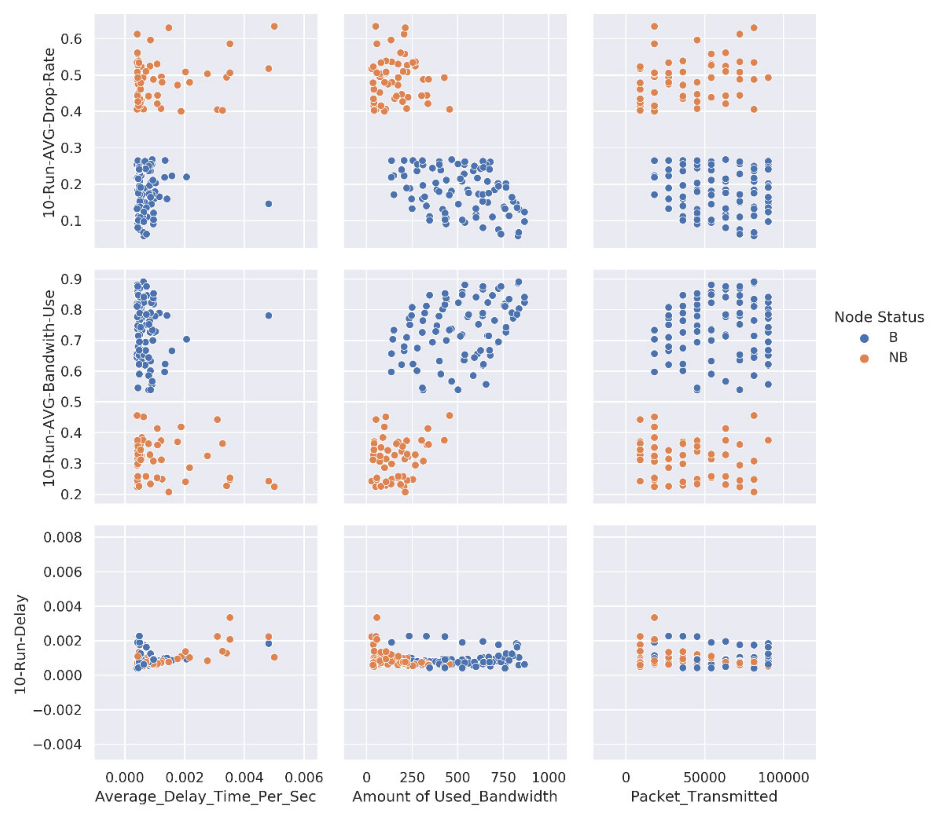
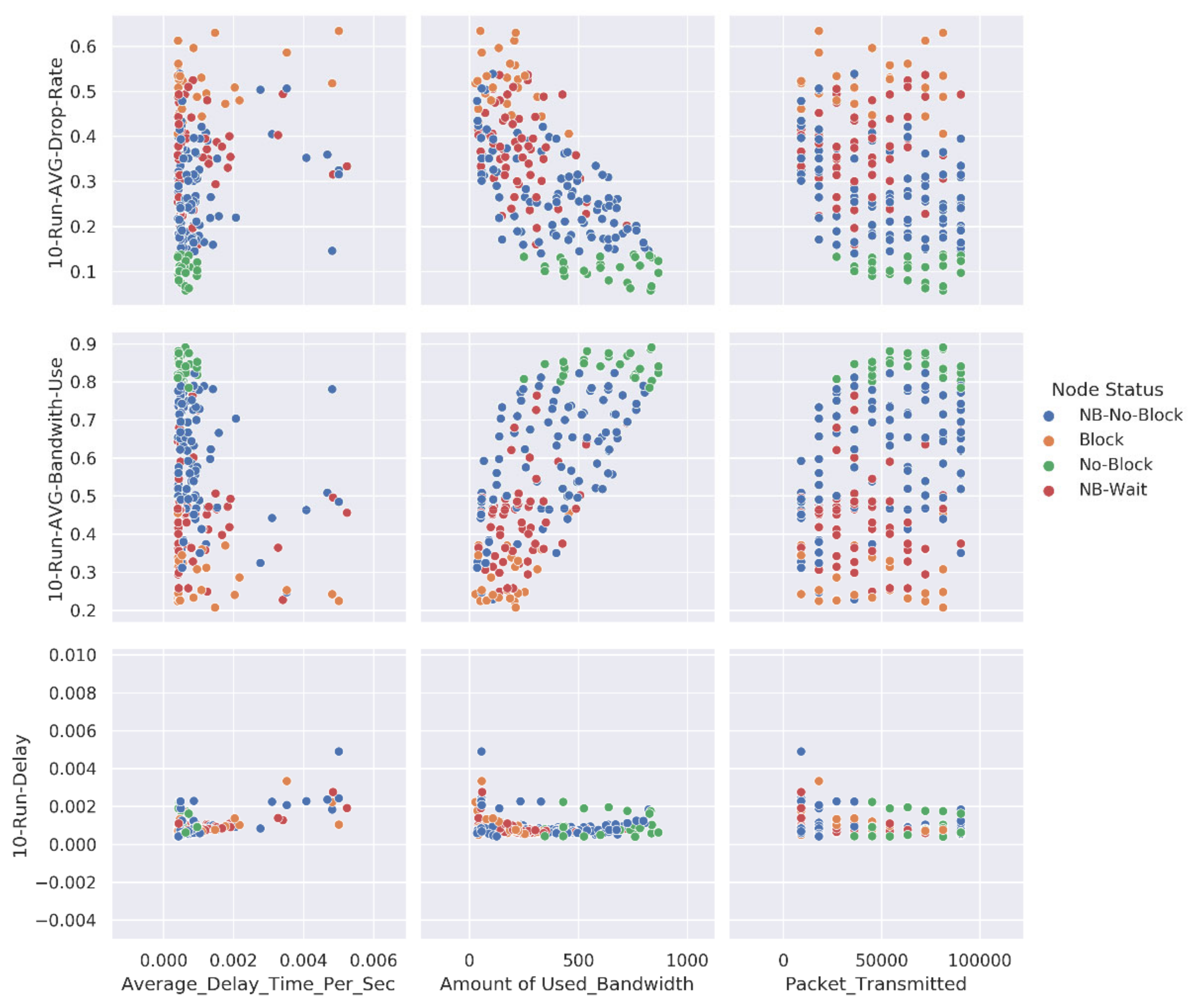
4.2. Dataset Preparation
- Average delay time per sec
- Amount of used bandwidth
- Packet transmitted
- Packet lost
- Received byte
- 10-run AVG drop rate
- 10-run delay
- 10-run AVG bandwidth use
- 10-run AVG drop rate
- 10-run delay
- 10-run AVG bandwidth use
4.3. Evaluation Metrices
4.4. Results and Analyses
5. Conclusions
Author Contributions
Funding
Institutional Review Board Statement
Informed Consent Statement
Data Availability Statement
Conflicts of Interest
References
- De Sanctis, M.; Bisio, I.; Araniti, G. Data mining algorithms for communication networks control: Concepts, survey and guidelines. IEEE Netw. 2016, 30, 24–29. [Google Scholar] [CrossRef]
- Ridwan, M.A.; Radzi, N.A.M.; Abdullah, F.; Jalil, Y.E. Applications of Machine Learning in Networking: A Survey of Current Issues and Future Challenges. IEEE Access 2021, 9, 52523–52556. [Google Scholar] [CrossRef]
- Boutaba, R.; Salahuddin, M.A.; Limam, N.; Ayoubi, S.; Shahriar, N.; Estrada-Solano, F.; Caicedo, O.M. A comprehensive survey on machine learning for networking: Evolution, applications and research opportunities. J. Internet Serv. Appl. 2018, 1–99. [Google Scholar] [CrossRef] [Green Version]
- Al-Shargabi, M. The impacts of burst assembly parameters on optical burst switching network performance. Int. J. Emerg. Trends Eng. Res. 2020, 8, 4916–4919. [Google Scholar] [CrossRef]
- Rajab, A.; Huang, C.T.; Alshargabi, M.; Cobb, J. Countering burst header packet flooding attack in optical burst switching network. In Proceedings of the International Conference on Information Security Practice and Experience, Zhangjiajie, China, 16–18 November 2016; Springer International Publishing: Berlin/Heidelberg, Germany, 2016; pp. 315–329. [Google Scholar]
- Hossain, M.K.; Haque, M.M. A Semi-Supervised Machine Learning Approach Using K-Means Algorithm to Prevent Burst Header Packet Flooding Attack in Optical Burst Switching Network. Baghdad Sci. J. 2019, 16, 804. [Google Scholar]
- Hossain, M.K.; Haque, M.M. A semi-supervised approach to detect malicious nodes in OBS network dataset using gaussian mixture model. In Lecture Notes in Networks and Systems; Springer: Singapore, 2020; Volume 89. [Google Scholar]
- Hossain, M.K.; Haque, M.M. Semi-supervised learning approach using modified self-training algorithm to counter burst header packet flooding attack in optical burst switching network. Int. J. Electr. Comput. Eng. 2020, 10, 4340–4351. [Google Scholar] [CrossRef]
- Jayaraj, A.; Venkatesh, T.; Murthy, C.S.R. Loss Classification in Optical Burst Switching Networks using Machine Learning Techniques: Improving the Performance of TCP. IEEE J. Sel. Areas Commun. 2008, 26, 45–54. [Google Scholar] [CrossRef]
- Levesque, M.; Elbiaze, H. Graphical Probabilistic Routing Model for OBS Networks with Realistic Traffic Scenario. In Proceedings of the IEEE Global Telecommunications Conference, Honolulu, HI, USA, 30 November–4 December 2009. [Google Scholar]
- Skorin-Kapov, N.; Chen, J.; Wosinska, L. A new approach to optical networks security: Attack-aware routing and wavelength assignment. IEEE/ACM Trans. Netw. 2010, 18, 750–760. [Google Scholar] [CrossRef]
- McGregor, A.; Hall, M.; Lorier, P.; Brunskill, J. Flow Clustering Using Machine Learning Techniques; Springer: Berlin/Heidelberg, Germany, 2004; pp. 205–214. [Google Scholar]
- Nguyen, T.T.T.; Armitage, G. A survey of techniques for internet traffic classification using machine learning. IEEE Commun. Surv. Tutor. 2008, 10, 56–76. [Google Scholar] [CrossRef]
- Sliti, M.; Boudriga, N. BHP flooding vulnerability and countermeasure. Photonic Netw. Commun. 2015, 29, 198–213. [Google Scholar] [CrossRef]
- Sliti, M.; Hamdi, M.; Boudriga, N. A novel optical firewall architecture for burst switched networks. In Proceedings of the 12th International Conference on Transparent Optical Networks, Munich, Germany, 27 June–1 July 2010. [Google Scholar]
- Rajab, A.; Huang, C.T.; Al-Shargabi, M. Decision tree rule learning approach to counter burst header packet flooding attack in Optical Burst Switching network. Opt. Switch. Netw. 2018, 29, 15–26. [Google Scholar] [CrossRef]
- Zahid Hasan, M.; Zubair Hasan, K.M.; Sattar, A. Burst header packet flood detection in optical burst switching network using deep learning model. Procedia Comput. Sci. 2018, 143, 970–977. [Google Scholar] [CrossRef]
- Lopez-Martin, M.; Carro, B.; Sanchez-Esguevillas, A. Variational data generative model for intrusion detection. Knowl. Inf. Syst. 2019, 60, 569–590. [Google Scholar] [CrossRef]
- Kingma, D.P.; Rezende, D.J.; Mohamed, S.; Welling, M. Semi-supervised learning with deep generative models. Adv. Neural Inf. Process. Syst. 2014, 4, 3581–3589. [Google Scholar]
- Li, Y.; Guan, C.; Li, H.; Chin, Z. A self-training semi-supervised SVM algorithm and its application in an EEG-based brain computer interface speller system. Pattern Recognit. Lett. 2008, 29, 1285–1294. [Google Scholar] [CrossRef]
- Wang, B.; Spencer, B.; Ling, C.X.; Zhang, H. Semi-supervised self-training for sentence subjectivity classification. In Lecture Notes in Computer Science (Including Subseries Lecture Notes in Artificial Intelligence and Lecture Notes in Bioinformatics); Springer: Berlin/Heidelberg, Germany, 2008. [Google Scholar]
- Tanha, J.; van Someren, M.; Afsarmanesh, H. Semi-supervised self-training for decision tree classifiers. Int. J. Mach. Learn. Cybern. 2017, 8, 355–370. [Google Scholar] [CrossRef] [Green Version]
- Sinaga, K.P.; Yang, M.S. Unsupervised K-means clustering algorithm. IEEE Access 2020, 8, 80716–80727. [Google Scholar] [CrossRef]
- Jain, A.K. Data clustering: 50 years beyond K-means. Pattern Recognit. Lett. 2010, 31, 651–666. [Google Scholar] [CrossRef]
- Marwala, T. Gaussian Mixture Models. In Handbook of Machine Learning; World Scientific: Singapore, 2018. [Google Scholar]
- Xuan, G.; Zhang, W.; Chai, P. EM algorithms of Gaussian mixture model and Hidden Markov Model. In Proceedings of the IEEE International Conference on Image Processing, Thessaloniki, Greece, 7–10 October 2001. [Google Scholar]
- Murphy, K.P. Mixture models and the EM algorithm. Mach. Learn Probabilistic Perspect. 2012, 1, 337. [Google Scholar]
- Riloff, E.; Wiebe, J.; Phillips, W. Exploiting subjectivity classification to improve information extraction. Proc. Natl. Conf. Artif. Intell. 2005, 1, 1106–1111. [Google Scholar]
- Zhu, X. Semi-Supervised Learning Literature Survey; University of Wisconsin-Madison: Madison, WI, USA, 2005. [Google Scholar]
- Geurts, P.; Ernst, D.; Wehenkel, L. Extremely randomized trees. Mach. Learn. 2006, 63, 3–42. [Google Scholar] [CrossRef] [Green Version]
- Kozodoi, N.; Katsas, P.; Lessmann, S.; Moreira-Matias, L.; Papakonstantinou, K. Shallow Self-learning for Reject Inference in Credit Scoring. In Lecture Notes in Computer Science; Springer: Cham, Switzerland, 2020; Volume 11908. [Google Scholar] [CrossRef]
- Blum, A.; Mitchell, T. Combining labeled and unlabeled data with co-training. In Proceedings of the Annual ACM Conference on Computational Learning Theory, Madison, WI, USA, 24–26 July 1998. [Google Scholar]
- Chan, T.F.; Golub, G.H.; LeVeque, R.J. Updating Formulae and a Pairwise Algorithm for Computing Sample Variances. In COMPSTAT 1982 5th Symposium Held at Toulouse 1982; Caussinus, H., Ettinger, P., Tomassone, R., Eds.; Physica: Heidelberg, Germany, 1982. [Google Scholar]
- Bentéjac, C.; Csörgő, A.; Martínez-Muñoz, G. A comparative analysis of gradient boosting algorithms. Artif. Intell. Rev. 2021, 54, 1937–1967. [Google Scholar] [CrossRef]
- Yu, H.F.; Huang, F.L.; Lin, C.J. Dual coordinate descent methods for logistic regression and maximum entropy models. Mach. Learn. 2011, 85, 41–75. [Google Scholar] [CrossRef] [Green Version]
- Kullarni, V.Y.; Sinha, P.K. Random Forest Classifier: A Survey and Future Research Directions. Int. J. Adv. Comput. 2013, 36, 1144–1156. [Google Scholar]
- Chen, T.; Guestrin, C. XGBoost: A scalable tree boosting system. In Proceedings of the ACM SIGKDD International Conference on Knowledge Discovery and Data Mining, San Francisco, CA, USA, 13–17 August 2016. [Google Scholar]
- Wang, X.; Li, X.; Ma, R.; Li, Y.; Wang, W.; Huang, H.; Xu, C.; An, Y. Quadratic discriminant analysis model for assessing the risk of cadmium pollution for paddy fields in a county in China. Environ. Pollut. 2018, 236, 366–372. [Google Scholar] [CrossRef]
- He, K.; Zhang, X.; Ren, S.; Sun, J. Delving deep into rectifiers: Surpassing human-level performance on imagenet classification. In Proceedings of the IEEE International Conference on Computer Vision, Santiago, Chile, 7–13 December 2015; pp. 1026–1034. [Google Scholar]
- Anaconda for Python. Available online: https://www.anaconda.com/distribution/ (accessed on 17 November 2019).
- Pedregosa, F.; Varoquaux, G.; Gramfort, A.; Michel, V.; Thirion, B.; Grisel, O.; Blondel, M.; Prettenhofer, P.; Weiss, R.; Dubourg, V.; et al. Scikit-learn: Machine learning in Python. J. Mach. Learn. Res. 2011, 12, 2825–2830. [Google Scholar]
- OBS Network Dataset. Available online: https://archive.ics.uci.edu/ml/datasets/Burst+Header+Packet+%28BHP%29+flooding+attack+on+Optical+Burst+Switching+%28OBS%29+Network (accessed on 9 January 2019).
- NCTUns Network Simulator and Emulator. Available online: http://www.estinet.com/ns/?page_id=21140 (accessed on 2 August 2021).
- Pourhashemi, S.M. E-mail spam filtering by a new hybrid feature selection method using Chi2 as filter and random tree as wrapper. Eng. J. 2014, 18, 123–134. [Google Scholar] [CrossRef] [Green Version]
- Mohammad, R.M.; Thabtah, F.; McCluskey, L. An improved self-structuring neural network. In Trends and Applications in Knowledge Discovery and Data Mining PAKDD 2016; Lecture Notes in Computer Science; Cao, H., Li, J., Wang, R., Eds.; Springer: Cham, Switzerland, 2016; Volume 9794. [Google Scholar]
- Ballabio, D.; Grisoni, F.; Todeschini, R. Multivariate comparison of classification performance measures. Chemom. Intell. Lab. Syst. 2018, 174, 33–44. [Google Scholar] [CrossRef]
- Natarajan, N.; Dhillon, I.S.; Ravikumar, P.; Tewari, A. Cost-sensitive learning with noisy labels. J. Mach. Learn. Res. 2018, 18, 5666–5698. [Google Scholar]


| Symbol | Meaning |
|---|---|
| X | Unlabeled dataset |
| x | single data point from X |
| k | number of clusters |
| Symbol | Meaning |
|---|---|
| μk | mean of k-th gaussian |
| Σk | variance of k-th gaussian |
| x | data point for dataset X, i.e., (xєX) |
| n | total data points in dataset X |
| k | mixture components |
| wik | probability that point xi is generated by the k-th Gaussian |
| Nk | i.e., the effective number of data points assigned to k-th Gaussian |
| πk | prior probability(weight) of k-th gaussian |
| Θk | (μk, Σk) |
| F(xi|Θk) | probability distribution of observation xi, parameterized on Θ |
| Algorithm Name | Modified Parameters |
|---|---|
| Gaussian Mixture Model | covariance_type= [‘spherical’, ‘diag’, ‘tied’, ‘full’], maximum iteration = 100, radom_state or seed = 120 |
| K-Means | No parameter modified |
| Extra Trees Classifier | random_state or seed = 120 |
| Random Forest Classifier | random_state or seed = 120 |
| XGBoost Classifier | random_state or seed = 120 |
| Gradient Boosting Classifier | random_state or seed = 120 |
| Gaussian | No parameter modified |
| Logistic Regression | maximum iteration = 1000, random_state or seed = 120 |
| Multi-Layer Perceptron Classifier | maximum iteration = 1500, random_state or seed = 120 |
| Quadratic Discriminant Analysis | No parameter modified |
| Sl. | Attribute name | Meaning |
|---|---|---|
| i. | Node | This is the label of edge node |
| ii. | Full bandwidth | This is a user allocated initial reserved bandwidth for an individual node. It is also called reserved bandwidth |
| iii. | Utilized bandwidth rate | The amount which can be reserved from the allocated bandwidth, i.e., from full bandwidth column |
| iv. | Packet drop rate | Packet drop rate for individual node, in percentage |
| v. | Percentage of lost packet rate | Packets drop rate, in percentage for individual node |
| vi. | Average delay time per sec | Average of delay per second for individual node |
| vii. | Packet received rate | Total packets received per second for individual node on the basis of reserved bandwidth |
| viii. | Percentage of lost byte rate | Lost byte rate, in percentage for individual node |
| ix. | Amount of used bandwidth | The amount each individual node could reserve from allocated bandwidth |
| x. | Packet size byte | Packets size allocated in byte for individual node to send |
| xi. | Received byte | This is the total byte received per second for an individual node on the basis of reserved bandwidth |
| xii. | Lost bandwidth | The lost amount of assigned bandwidth |
| xiii. | 10-run-avg- drop-rate | This is the average of packet drop rate for ten successive iterations in simulation |
| xiv. | 10-run-delay | The average of delay time for 10 successive iterations in simulation |
| xv. | 10-run-avg- bandwidth use | This is the average of bandwidth utilized for 10 successive iterations in simulation |
| xvi. | Packet transmitted | The amount of total packets transmitted per second for individual node on the basis of allocated bandwidth |
| xvii. | Packet received | The amount of total packets received per second for individual node on the basis of reserved bandwidth |
| xviii. | Packet lost | The amount of total packets lost per second for individual node on the basis of lost bandwidth |
| xix. | Transmitted byte | Total bytes transmitted per second for individual node |
| xx. | Flood status | The amount of flood per node, in percentage on the basis of packet drop rate |
| xxi. | Node Status | The classification of nodes into one of three classes, behaving, potentially not behaving, and not behaving |
| xxii. | Class | It is the classification of the nodes into one of four classes; NB-No- Block, block, NB-wait, no-block |
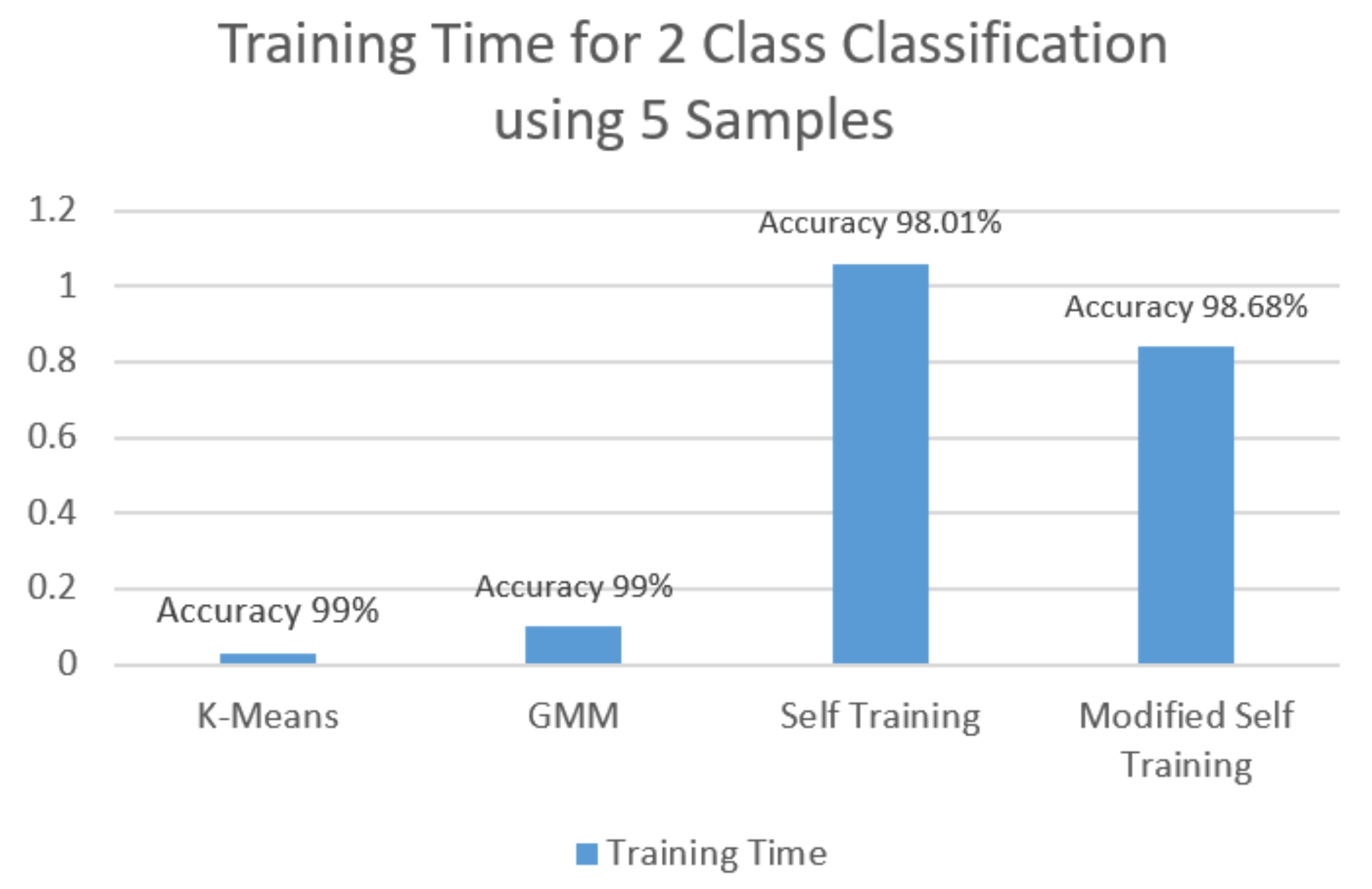
| SSML Method | Accuracy | F1 | Precision | Recall |
|---|---|---|---|---|
| K-means- based | 99 | 0.992 | 1.000 | 0.99 |
| GMM-based | 99 | 0.992 | 1.000 | 0.99 |
| ST | 98.013 | 0.973 | 1.000 | 0.947 |
| MST | 98.675 | 0.982 | 1.000 | 0.965 |
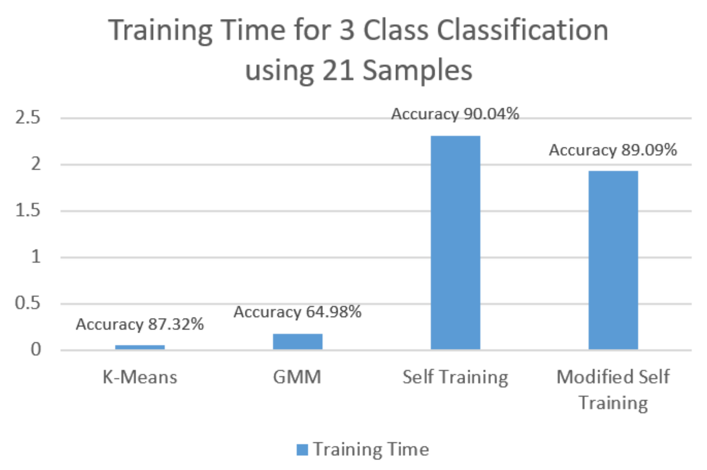
| SSML Method | Accuracy | F1 | Precision | Recall |
|---|---|---|---|---|
| K-means-based | 87.32 | 0.879 | 0.890 | 0.891 |
| GMM-based | 64.98 | 0.631 | 0.619 | 0.819 |
| ST | 90.038 | 0.779 | 0.923 | 0.728 |
| MST | 89.089 | 0.784 | 0.818 | 0.762 |
| SSML Method | Accuracy | F1 | Precision | Recall |
|---|---|---|---|---|
| K-means-based | 55.69 | 0.576 | 0.569 | 0.701 |
| GMM-based | 54.86 | 0.573 | 0.575 | 0.696 |
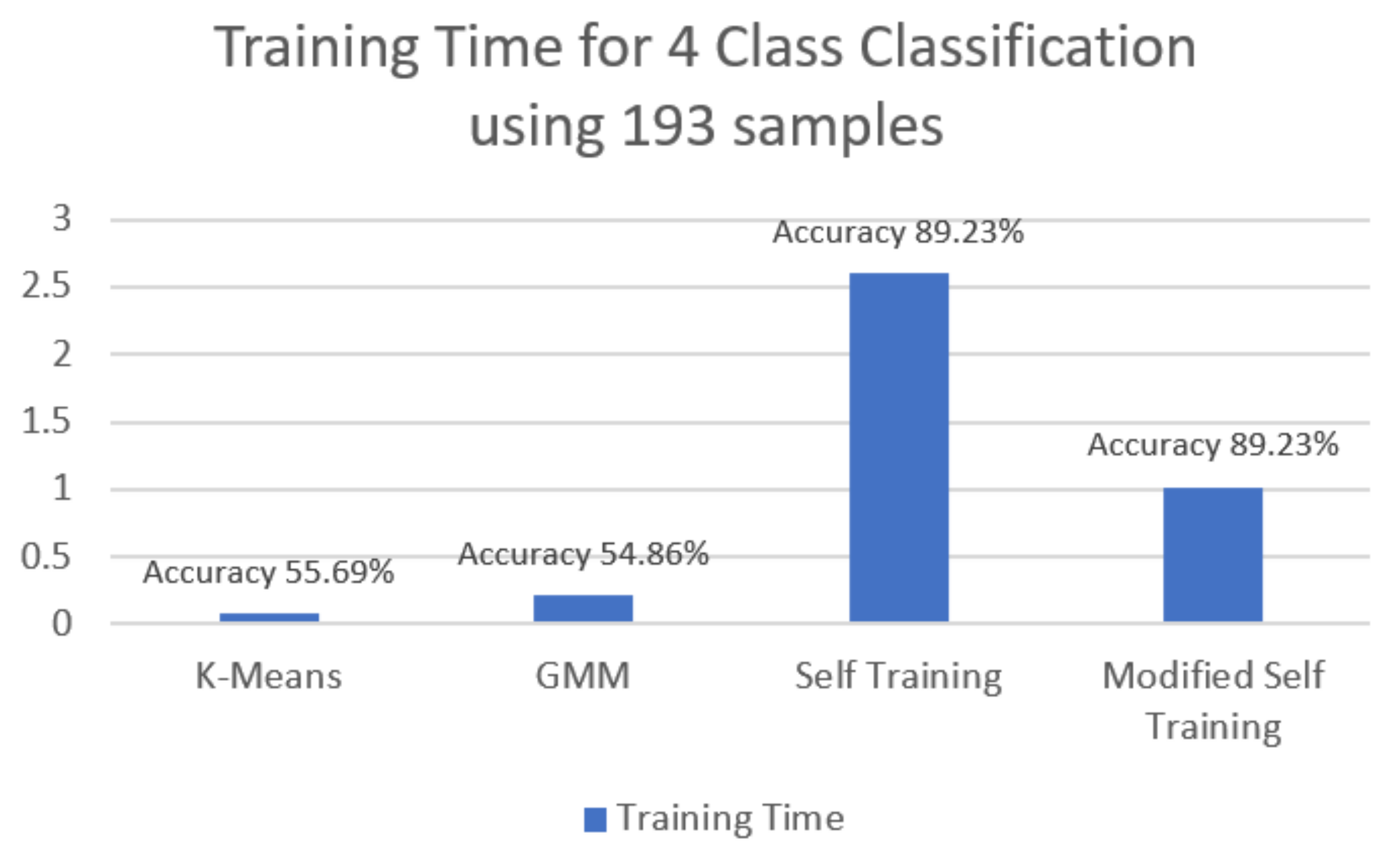
| ST | 89.229 | 0.889 | 0.879 | 0.903 |
| MST | 89.229 | 0.893 | 0.884 | 0.905 |
| Works | ML Method | Detection Accuracy (in Percentage) and the Amount of Truly Labeled Instances Used | ||
|---|---|---|---|---|
| In Detecting Two Classes (B, NB) | In Detecting Three Classes (B, NB, PNB) | In Detecting Four Classes (Block, No-Block, NB-Wait, NB-No-Block) | ||
| Rajab et al. [16] | Decision tree rule learning | 93% accurate using 1075 truly labeled instances | NA | 87% accurate using 1075 truly labeled instances |
| Hasan et al. [17] | Deep neural networks | NA | NA | 99% accurate using 1060 truly labeled instances |
| Based on Kamrul et al. [6] | K-means based SSML | 99% accurate using 5 truly labeled instances | 87.32% accurate using 21 truly labeled instances | 55.69% accurate using 193 truly labeled instances |
| Based on Kamrul et al. [7] | GMM-based SSML | 99% accurate using 5 truly labeled instances | 64.98% accurate using 21 truly labeled instances | 54.86% accurate using 193 truly labeled instances |
| Based on Kamrul et al. [8] | Self-training | 98.01% accurate using 5 truly labeled instances | 90.04% accurate using 21 truly labeled instances | 89.23% accurate using 193 truly labeled instances |
| Based on Kamrul et al. [8] | Modified self-training | 98.68% accurate using 5 truly labeled instances | 89.09% accurate using 21 truly labeled instances | 89.23% accurate using 193 truly labeled instances |
Publisher’s Note: MDPI stays neutral with regard to jurisdictional claims in published maps and institutional affiliations. |
© 2021 by the authors. Licensee MDPI, Basel, Switzerland. This article is an open access article distributed under the terms and conditions of the Creative Commons Attribution (CC BY) license (https://creativecommons.org/licenses/by/4.0/).
Share and Cite
Hossain, M.K.; Haque, M.M.; Dewan, M.A.A. A Comparative Analysis of Semi-Supervised Learning in Detecting Burst Header Packet Flooding Attack in Optical Burst Switching Network. Computers 2021, 10, 95. https://0-doi-org.brum.beds.ac.uk/10.3390/computers10080095
Hossain MK, Haque MM, Dewan MAA. A Comparative Analysis of Semi-Supervised Learning in Detecting Burst Header Packet Flooding Attack in Optical Burst Switching Network. Computers. 2021; 10(8):95. https://0-doi-org.brum.beds.ac.uk/10.3390/computers10080095
Chicago/Turabian StyleHossain, Md. Kamrul, Md. Mokammel Haque, and M. Ali Akber Dewan. 2021. "A Comparative Analysis of Semi-Supervised Learning in Detecting Burst Header Packet Flooding Attack in Optical Burst Switching Network" Computers 10, no. 8: 95. https://0-doi-org.brum.beds.ac.uk/10.3390/computers10080095