
An Experimental Study on Centrality Measures Using Clustering


1
Department of Information Systems, ELTE Eötvös Loránd University, 1117 Budapest, Hungary
2
Department of Informatics, J. Selye University, 94501 Komárno, Slovakia
*
Author to whom correspondence should be addressed.
Computers 2021, 10(9), 115; https://0-doi-org.brum.beds.ac.uk/10.3390/computers10090115
Submission received: 3 July 2021
/
Revised: 6 September 2021
/
Accepted: 12 September 2021
/
Published: 15 September 2021
Abstract
:Graphs can be found in almost every part of modern life: social networks, road networks, biology, and so on. Finding the most important node is a vital issue. Up to this date, numerous centrality measures were proposed to address this problem; however, each has its drawbacks, for example, not scaling well on large graphs. In this paper, we investigate the ranking efficiency and the execution time of a method that uses graph clustering to reduce the time that is needed to define the vital nodes. With graph clustering, the neighboring nodes representing communities are selected into groups. These groups are then used to create subgraphs from the original graph, which are smaller and easier to measure. To classify the efficiency, we investigate different aspects of accuracy. First, we compare the top 10 nodes that resulted from the original closeness and betweenness methods with the nodes that resulted from the use of this method. Then, we examine what percentage of the first n nodes are equal between the original and the clustered ranking. Centrality measures also assign a value to each node, so lastly we investigate the sum of the centrality values of the top n nodes. We also evaluate the runtime of the investigated method, and the original measures in plain implementation, with the use of a graph database. Based on our experiments, our method greatly reduces the time consumption of the investigated centrality measures, especially in the case of the Louvain algorithm. The first experiment regarding the accuracy yielded that the examination of the top 10 nodes is not good enough to properly evaluate the precision. The second experiment showed that the investigated algorithm in par with the Paris algorithm has around 45–60% accuracy in the case of betweenness centrality. On the other hand, the last experiment resulted that the investigated method has great accuracy in the case of closeness centrality especially in the case of Louvain clustering algorithm.
1. Introduction
In recent years, networks have become part of everyday life, and because of this, they became of high interest to researchers. With the development of computer science, large graphs took on essential roles in many scientific areas such as biology [1], chemistry [2], computer science [3], social engineering [4,5], marketing [6,7] or controlling disease spread. Nowadays, the use of graph databases is also becoming more common and popular, since many areas can take advantage of the benefits provided by graph structure and graph databases. Today’s popular social sites such as Facebook, Twitter, and Instagram use graphs to model relationships, which greatly speeds up queries about individual relationships, and network maintenance provides a unified interface for fast and efficient storage of relations. Furthermore, they are playing an increasing role in other areas of IT, such as telecommunications [8], road network infrastructure [9], and the organization of public transport routes [10]. In addition, they are gaining ground, for example, in biology, ref. [11] collected a large number of applications where significant breakthroughs have been achieved in the use of graph databases in biology.
In this paper, we use a method that uses different clustering algorithms to improve the computation of the mentioned centrality measures over large networks. Graph clustering uses different attributes of a graph to find dense communities that belong to the same group. Based on the clusters, the original graph can be divided into multiple subgraphs that are smaller in extent. Using different centrality measures on such subgraphs results in faster execution and less computation cost.
Related Work
Social network analysis and its applications is a fundamental and practical mathematical topic at the moment. There are numerous subjects in this field such as finding the shortest path between two nodes or finding k-dense subgraphs and so on. One of the most researched aspects of network analysis is finding the most important nodes and do it effectively. Since the idea of centrality was proposed, numerous methods have been introduced to measure a node’s centrality and rank the nodes based on this value. Each of these methods takes different aspects of the network to decide if a node is ’vital’ or not, thus each method has its limitations and drawbacks. One such algorithm is betweenness centrality [12], which is based on the number of shortest paths that go through a node. Closeness centrality ranks the nodes based on the average length of the shortest path between the node and all the other nodes in the network [13]. Another common measure is Eigenvector centrality [14] where the score of a node is influenced by the scores of its adjacents nodes based on the principle that nodes with high scoring neighbors have a larger score. PageRank [15] is also a well-known measure. It assigns a weight to each document based on the number of their incoming links. A bunch of algorithms was developed over time to calculate these values efficiently [16]; however, these were not scaling well on massive networks.
The identification of the vital nodes can be very time-consuming. Up to this point, research was conducted to decrease the runtime of the centrality algorithms. In [17], the authors propose parallel versions of betweenness and closeness centrality that can handle dynamic graphs, where nodes and edges could change in every time step. To access this problem they process a batch of updates in a parallel way. Another method was proposed in [18] that approximates centrality values with the aid of machine learning and node embedding. Their algorithm takes a set of features for each node and the adjacency matrix as its input and uses them to estimate the centrality rank of each node. In [19], they propose a lossy graph reduction approach that reduces the execution time of the centrality algorithms. After our investigations in this field, we decided to extend our previous research [20] and investigate the ranking efficiency and execution time of more centrality measures using clustering methods. Markov clustering [21] is a popular algorithm that is commonly used to cluster protein sequences in bioinformatics data [22]. It also can be used in a distributed form [23]. It is based on the random walk principle, which means if you randomly walk between nodes you are more likely to move around nodes in the same cluster instead of crossing to other clusters. The Louvian [24] method was designed to extract communities from large graphs. It is based on the idea of modularity optimization. Modularity is a value between 1 and −0.5 that is used to measure the relative density of the links in communities. The optimization of this value hypothetically results in the best clustering of the nodes. Paris algorithm is a hierarchical clustering algorithm that was proposed in [25]. It is an agglomerative method, which means that it performs a greedy merge on the nodes based on their similarity.
We investigate the runtime of the methods with and without the use of clustering algorithms. We also compare the top 10 nodes produced by the centrality measures on the original and the clustered graphs to gain insight into the accuracy of our method. The more the top nodes are alike, the more the result is similar to the original method. The use of graph databases can significantly reduce the runtime of calculations related to graphs. For example, researchers found out using a graph database over a relational database can find the best scoring path between two proteins approximately a thousand times faster and obtain the shortest paths significantly quicker; therefore, the conclusion is that the graph databases are ready for bioinformatics and can provide essential speedups on selected problems over relational databases. Accordingly, we considered it important to implement our method using graph databases as well, to make suggestions for problems that arise during implementation and use, and how to store different graphs in a database. Because of this, we also investigate if the runtime can be further accelerated via the use of a graph database.
2. Basic Concepts and Algorithms
In this section, we detail the used centrality measures. A high-level overview of the graph clustering algorithms can be also found here.
2.1. Betweenness Centrality
Betweenness centrality was introduced in [12] and is based on the shortest paths. It is defined as follows:
where is the betweenness centrality value of node i, is the total number of the shortest paths from node s to node t and is the number of those paths that pass through node i.
2.2. Closeness Centrality
Alex Bavelas (1950) [13] defined closeness as the reciprocal of the farness. It indicates the average length of shortest paths between a node and all the other nodes is a graph. It is defined as:
where is the closeness centrality score of node i and is the distance between nodes i and j, which is the number of edges in a shortest path that connects them.
2.3. Graph Clustering
With the use of graph clustering, the nodes of an enormous graph can be divided into multiple clusters based on different attributes such as neighborhood similarity or connectivity. With the use of graph clustering methods, densely connected groups or natural groupings of nodes can be found. A brief overview of the used algorithms can be read below.
2.4. Louvain Algorithm
Modularity was defined by Newman and Girvan in [26]. It is a scalar value between and 1 that is used to measure to compare the links between communities with the density of links inside communities. More formally,
where m is the sum of all of edge weights in the graph, and are the sum of the weights of the edges attached to nodes i and j, respectively, represents the edge weight between nodes i and j, and are the communities of the nodes and is Kronecker delta function ( if , 0 otherwise).
The nature of partitions that were collected by different methods can be compared with the use of modularity. Louvain clustering is capable of discovering partitions with high modularity. Other than that, it can also unfold the network’s complete hierarchical composition. Louvain algorithm consists of two steps that are repeated after one another. The algorithm takes a weighted G graph with N nodes as its input. First, every node is assigned to a different community, which results in N communities. Next, the modularity gain is calculated for each i node. It is achieved by deleting i from its community and assigning it to a community of j where j is a neighboring node to i. The modularity gain is calculated as follows:
where is the sum of the weights of the links inside community C, is the sum of the weights of the links from i to nodes in C and m is the sum of the weights of all links in the network, is the sum of the weights of the links incident to nodes in C and is the sum of the weights of the links incident to node i.
After this is calculated for all communities that contain i, it is reassigned to the community that achieved the largest modularity increase. Node i stays in its own community if there is no other community with a modularity increase. The process is applied for all nodes of G and repeated until no modularity increase can be accomplished.
The second step groups each community’s nodes and creates a new network, from the nodes inside a group. The edges between nodes in the same group are represented as self-loops, while weighted edges between the communities are used to indicate links between nodes that are in different communities.
2.5. Markov Algorithm
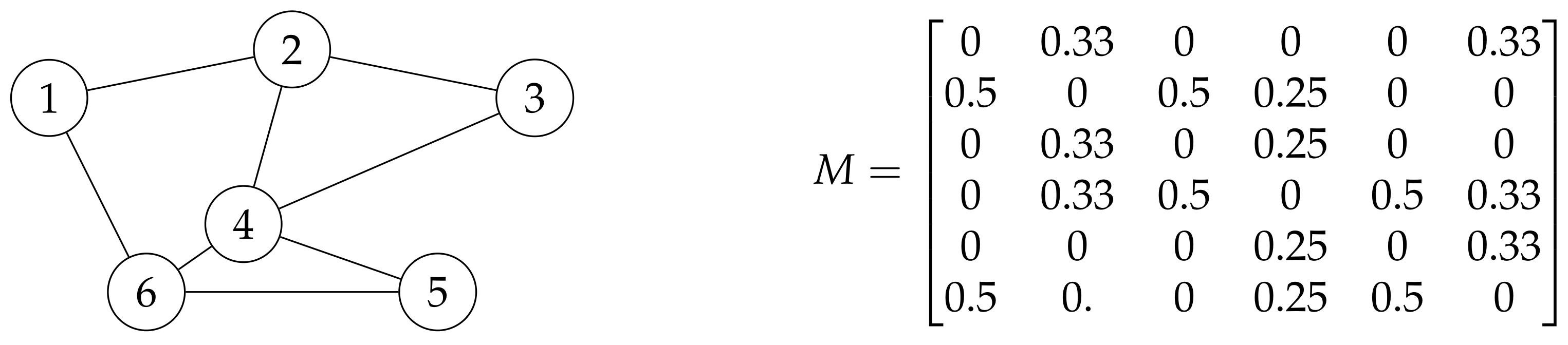
A matrix A is a Markov matrix if its entries are greater or equal to zero and the sum of each column’s entries is one. In this matrix, each entry represents transition probabilities from one state to another. Let G be a graph. Now let us place an object at vertex . At each iteration, the object has to move to a neighboring node. The probability that it moves to vertex is denoted as:
where represents the probability that a random walk of length k starting at vertex , ends at vertex , where the length is the number of edges. Random walk is a special case of the Markov chain, using transition probability matrices. With the use of random walks on a graph positions where flow converge can be found. Such positions indicate the existence of a cluster. All of the graph clustering algorithms are based on this principle. An example Markov matrix can be seen in Figure 1.
Let r be a non-negative number, and let be the initial Markov matrix. With the re-scaling of every column of M with the power coefficient r we acquire an . The inflation operator with power coefficient r is denoted as . The re-scaling is based on and . We use the inflation operator to weaken and strengthen the flow. The intensity of these effects is determined by the r parameter. There is another parameter, called expansion, which allows the flow to reach different regions of the graph. Expansion is calculated as . Markov chains and their transition matrix can be used to find different parts of the graph. The algorithm converges to a “doubly idempotent” matrix. This matrix only contains one value in each column and is considered to be in a steady state. Based on their relation to each other, nodes could be in two states. It can either attract other nodes or be attracted to another node. The nodes that attract others must have at least one positive value in their row in the final matrix. These nodes attract the other nodes in their row. Nodes that attract each other are considered to be in the same cluster.
In summary, an adjacency matrix is created, which is then altered by the probability matrices. After that, the matrix is inflated with the parameter r. These steps are repeated until a steady state is found. From this state, the clusters are obtained.
2.6. Paris
To understand the Paris algorithm, let us introduce some essential concept. A G graph’s weighted adjacency matrix A is a non-negative, symmetric matrix. If there is an edge between i and j then the corresponding value in the matrix is the weight of the edge that is between i and j. The weight of node i is:
which is the sum of the weights of its incident edges. The cumulative weight of G’s nodes is:
The weights can be used as a probability distribution on node pairs
and also on nodes
The distance of nodes i and j can be calculated with the use of the node pair sampling ratio
The node distance can be defined with the following conditional probability as well
which means that the distance between nodes i and j can be calculated as
Let us consider a cluster C on the graph G, and let a and b be two different clusters. All of the above equation applies to clusters as well, which means that the distance of a and b can be defined as
Paris algorithm merges the closest clusters based on this distance.
The algorithm works in the same way as the Louvain algorithm. First, a cluster is created for each node in G. The algorithm merges the two closest clusters until no modularity gain can be achieved. Probability can also be applied to the modularity defined in Section 2.4:
3. The Algorithm
In this section, we explain our algorithm that we proposed in [20] and is used in our experiments. Let G be an undirected graph with N nodes. The algorithm consists of two main stages. First, the clusters of G are created via the use of a clustering algorithm. The output is a mapping for each node where the keys represent the cluster labels, and the values represent the nodes that are associated with that cluster. The cluster mappings are saved in a JSON format, so they can be reused in experiments in the future.
In the second phase, we create sub-graphs of the original G graph based on the clusters that were created in the previous step. The betweenness and closeness centrality are then calculated on these sub-graphs. After the calculation of the centrality values on the sub-graphs, the values are assigned to the nodes of the original graph. Because that these sub-graphs are smaller in magnitude than the original G graph, the use of the centrality measures becomes a cost-effective subproblem.
Due to the loss of the edges between sub-graphs, our algorithm only gives an approximate solution of the measures compared to the calculation on the whole graph; therefore, the centrality values calculated by our method might differ from the values obtained by centrality algorithms on the complete graph. Our experiments yielded that the proposed algorithm in [20] is accurate in the case of closeness centrality, scales well, and is able to determine influential nodes up to 20 times faster than traditional centrality measures.
It is crucial to know that the Markov clustering highly depends on its expansion and inflation parameter. Because of that, we experimented with values between to find an ideal value for the algorithm.
In this paper, we expanded the range of the centrality algorithms, which were examined previously. Since graph databases could store and process graph data more efficiently, we also proposed a solution on how to apply this technique in a Neo4j Graph Database using Cypher queries. The experiments we conducted proved that our algorithm can be used to reduce the execution time of the centrality measures significantly; however, it has only around 45–60% accuracy in the case of betweenness centrality if the top n are compared. If the sum of the values of the nodes is being examined, the investigated method used with Louvain clustering properly approximates the original closeness centrality measure.
4. Graph Databases
A graph database is a database management system that has the standard CRUD (Create, Read, Update, Delete) operations, and uses graph structures that consist of nodes, edges, and properties to represent and store data. The same structure is used for semantic queries. Graph databases are NoSQL databases, which are optimized for transactional performance and engineered with transactional integrity and availability in mind. There are two properties that might differ in graph databases: the underlying storage and the processing engine. Some graph databases use relational databases, object-oriented databases, or even some general-purpose data storage systems to serialize and store the graph data, while others use native graph storage that is optimized and designed for not just storing but managing graphs. Numerous graph databases use native graph processing engines that rely on the index-free adjacency property that enforces the nodes to have a direct physical RAM address and physically point to other adjacent nodes resulting in a fast traversal of the graph. For our experiments we used Neo4j; in the next subsection, we go through its fundamental concepts.
4.1. Neo4J
The Neo4J (Network Exploration and Optimization 4 Java) is a graph database management system that offers ACID-compliant transactions and native graph data storage and processing. Neo4J uses the property graph model to store information. The entities are called nodes that can hold an arbitrary number of properties which are key–value pairs. A node can have multiple labels indicating the role of the node. With the use of these labels, constraints and indices can be created.
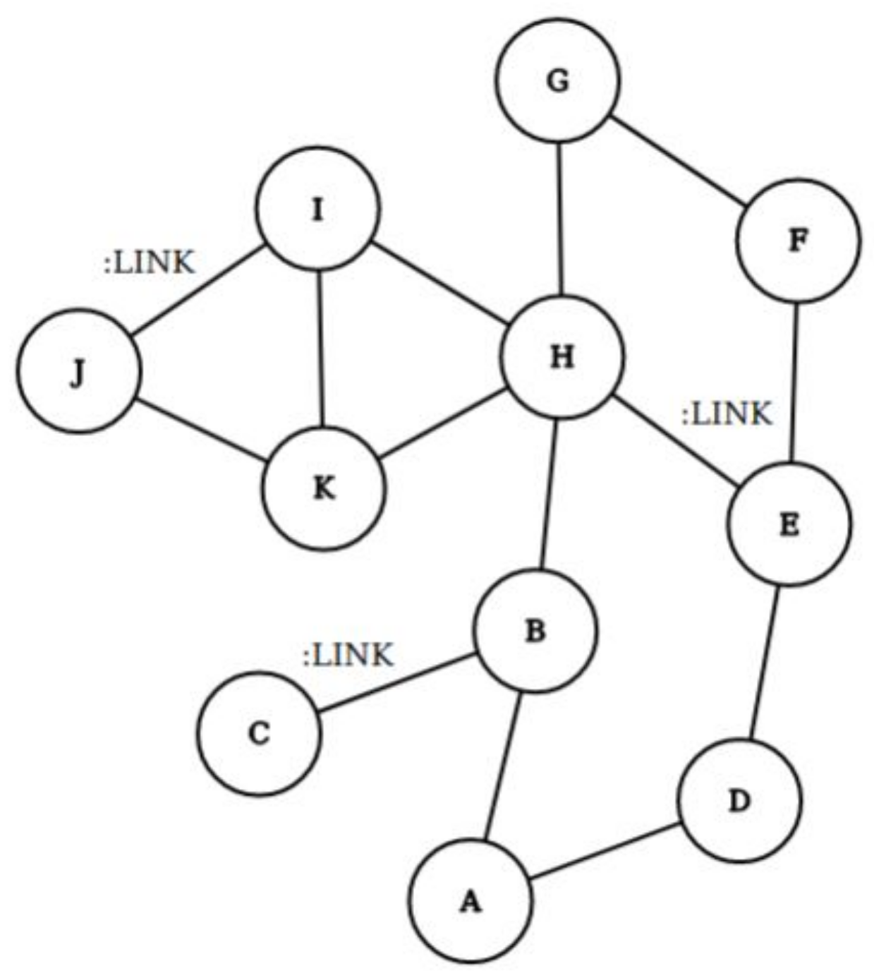
In Neo4j, relationships are represented as directed connections between two nodes. These links must have a type, a start node, and an end node. Similar to nodes, relationships can also have properties. Between two nodes, there can be any number or type of relationship without performance loss. Despite the directed relationships, relationships can be traversed efficiently in either direction. Figure 2 visualizes a property graph. A to K are the nodes, and “:LINK” represents the connection between two nodes. To avoid congestion, only three “:LINK” are printed out in the figure; however, each edge without “:LINK” is a full value connection.
4.2. Cypher
Cypher is a declarative graph query language that enables expressive and powerful querying of data on a property graph. The language was designed to be easily read and understood by the user while keeping the power and capability of SQL (standard query language). Cypher allows running queries to find data that match a specific pattern. The language’s syntax is based on ASCII art, which makes the queries readable and very visual. Cypher, such as other query languages contains several keywords to define patterns, filter patterns, and return results. The most common keywords are MATCH, WHERE, and RETURN, which act differently than the usual SELECT, …, WHERE statement, although they have a similar purpose.
4.3. Graph Data Science Library
Graph Data Science (GDS) library [28] is a graph processing framework. GDS provides parallel versions of graph algorithms for Neo4j, exposed as Cypher procedures. The library already has efficiently implemented the betweenness and closeness algorithms that we applied in our solution. To run these algorithms, the GDS library uses a specially designed in-memory graph format to represent the graph data. This means that the data from the database need to be loaded into an in-memory graph catalog. Regulation of the amount of data loaded by graph projections is possible, which allows filtering on nodes and relationships based on a property or a label. We use the latter to filter the nodes that have the same cluster ID and create the corresponding subgraph. The projections of the subgraphs are stored in memory using compressed data structures that are optimized for topology and property lookup operations. GDS has two variants of projecting a graph from the database to the memory: native projection and Cypher projection. The native projection provides better performance since under the hood it uses the internal Neo4J API, which results in faster graph loading; however, it is limited only to specifying node labels and relationship types. Due to this limitation, it is not suitable for our proposed algorithm. Cypher projection, on the other hand, is a more flexible, expressive approach that supports all the features of the Cypher query language and can be used to filter nodes that belong to the same group.
By default, for the Cypher projection, the graph must have a name for later reuse; however, due to the clustering algorithm, we might need to create several subgraphs that would only be used when the algorithm is running, and there is no need for reuse; GDS provides so-called anonymous graphs to remedy this. The anonymous graph can be specified with two parameters: nodeQuery and relationship Query. These parameters are used to create constraints on the nodes and relationships. This enables us to select specific parts of the graph.
Once a graph is loaded into the database the implemented centrality measures can be used. They calculate the values on the projection of the subgraph. In the end, we aggregate the partial results to obtain the centrality values for the whole graph.
5. Clusters and Parameters
5.1. Cluster Creation
For our experiments, we selected three graph clustering methods, namely Louvain, Markov, and Paris, which, although based on different methods, have a common goal: finding communities within a large graph. These clustering algorithms usually have parameters that notably influence the output of an algorithm. Choosing the optimal parameters is not always trivial or even possible, however, the algorithms are highly sensitive to the choice of their parameter values. The goal of these parameters was to resolve complications that were introduced by structural properties such as varying densities. From the selected algorithms, the Markov algorithm has parameters that can fine-tune the outcome of the algorithm. The Louvain and Paris algorithms do not require any parameters. It is important to know that, in the case of large graphs, trying out clustering parameter values is not computationally feasible. Because of this, we give a brief overview of our parameter selection that is based on the researcher’s recommendations.
5.2. Markov Parameters
As we explained in Section 2.5, the Markov algorithm has two major parameters: inflation and expansion. Inflation has a correlation with the granularity of the resulting output. A higher r value can result that the flow will reach longer distances in the input graph; therefore, inflation is the key parameter of the algorithm, while the expansion parameter is responsible for allowing the flow to connect different regions of the network.
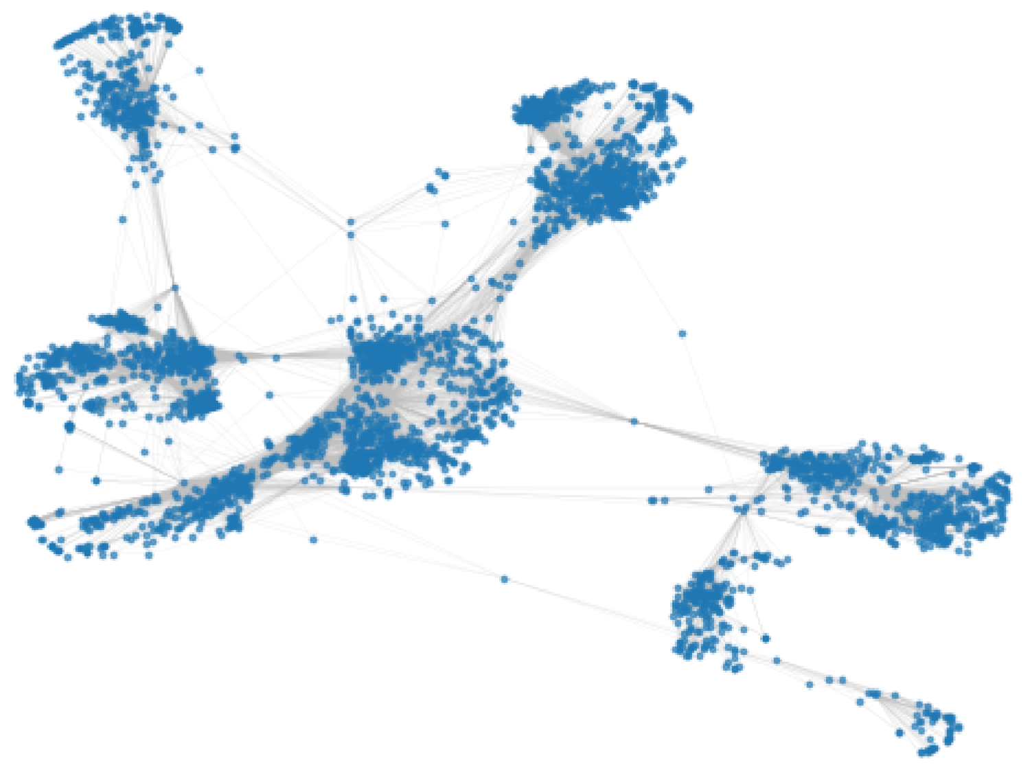
Modularity is a generally used metric to measure how effectively a network can be partitioned into communities, thus it can be used to optimize clustering parameters. Before we finalized our parameter selection, we performed multiple runs of the Markov algorithm using different inflation values from 1.5 to 2.5 inspired by [29]. To illustrate these processes, we will show the experimental results on the fb-combined social network, that consists of 4039 nodes and 88,234 edges.
As shown in Table 1, the inflation value of 1.8 produced the highest modularity value, which suggests higher clustering quality; therefore, we used this value in our final experiments. In the next phase, we focused on the expansion parameter, so we applied the same testing method where we picked values from 2 to 5 for the expansion, and we set the previously calculated inflation value. We obtained our results with the use of the NetworkX library, which by default produces a result with the precision of seven decimal places. Based on our experiments we experienced that in the case of large networks, the modularity values can be very similar, so examination of all these digits is necessary.
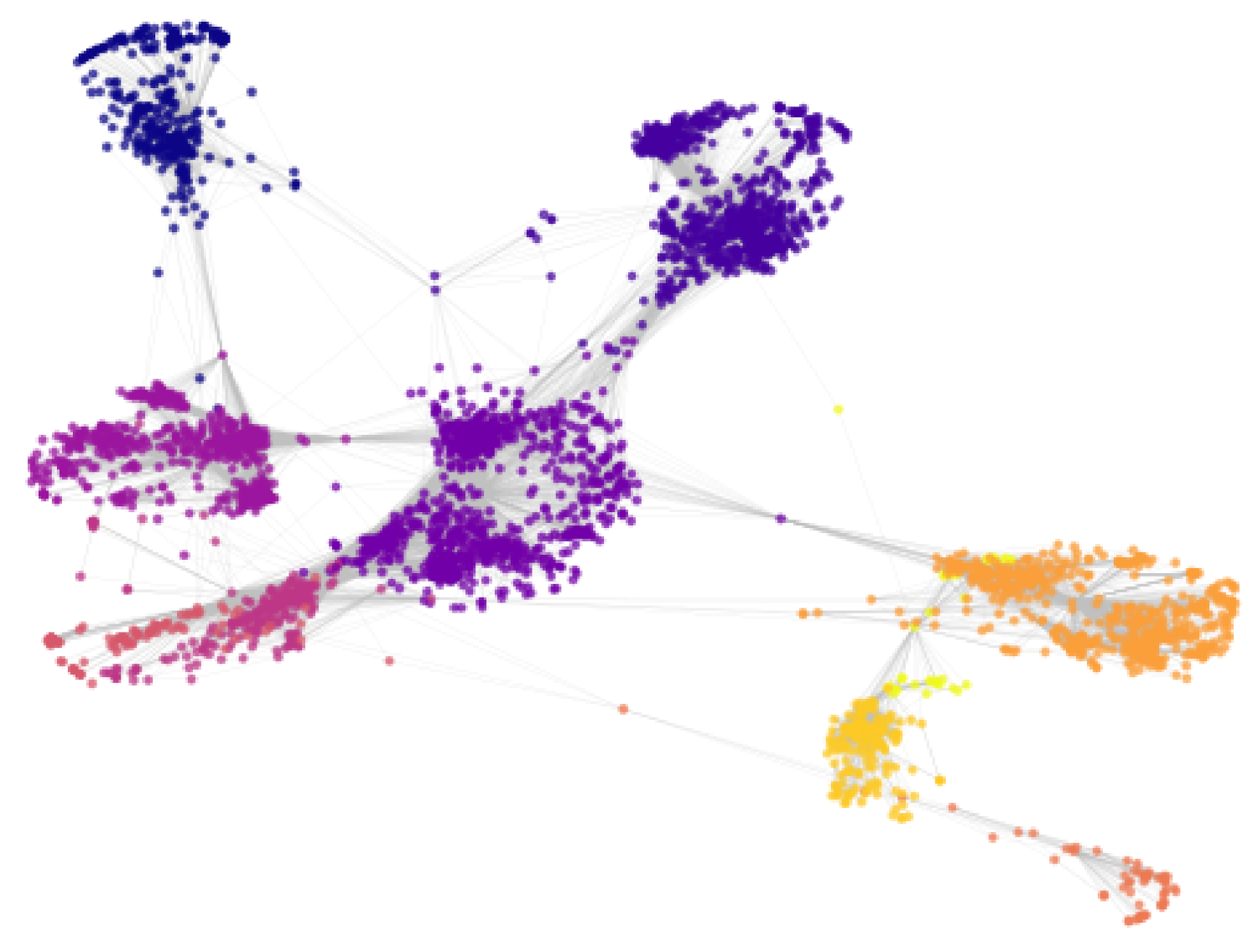
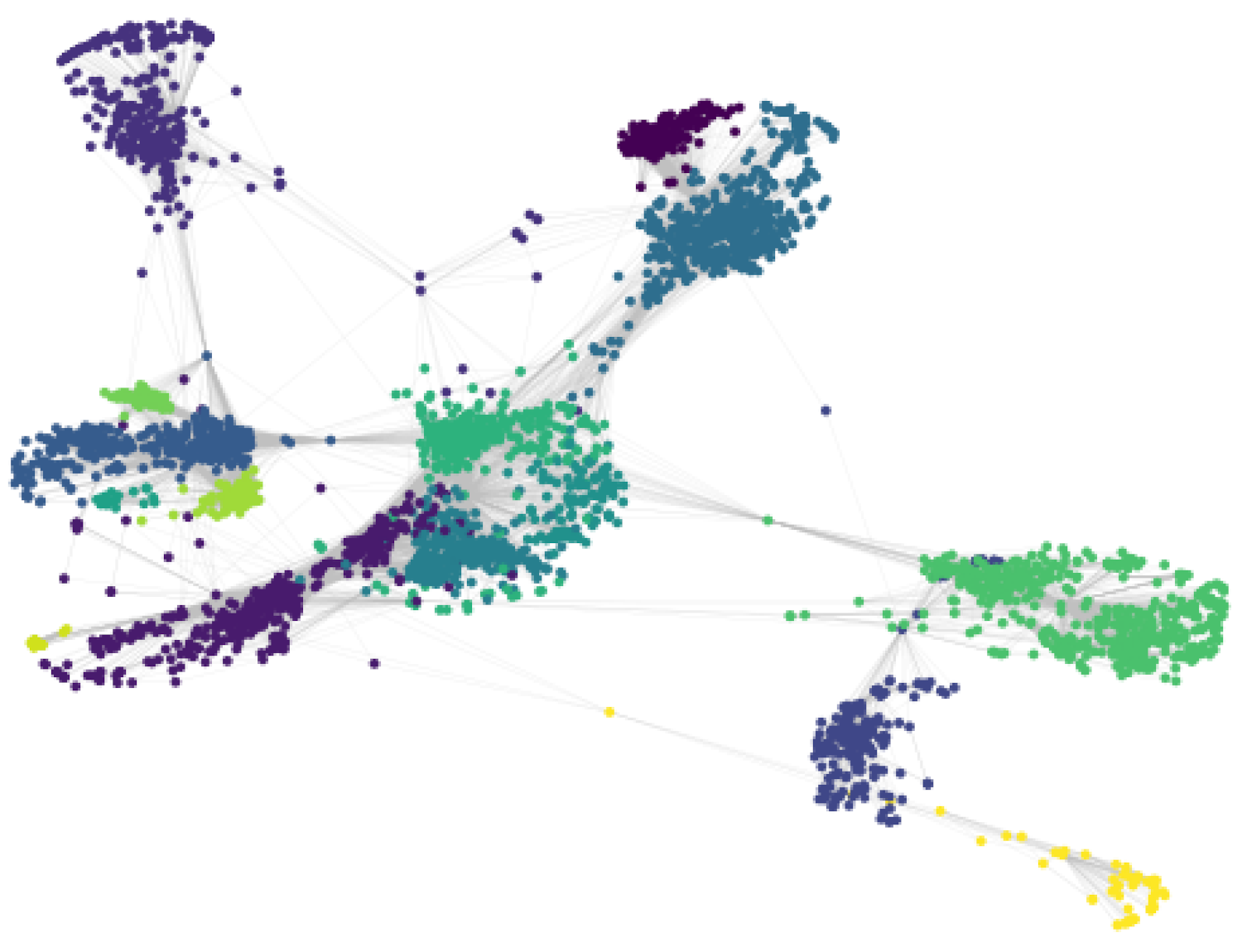
Table 2 shows that we were able to obtain the highest modularity score with the value of 2. With this knowledge, we obtained 10 clusters from the facebook_combined network using the Markov clustering algorithm. Each color represents a separate cluster in the graph.
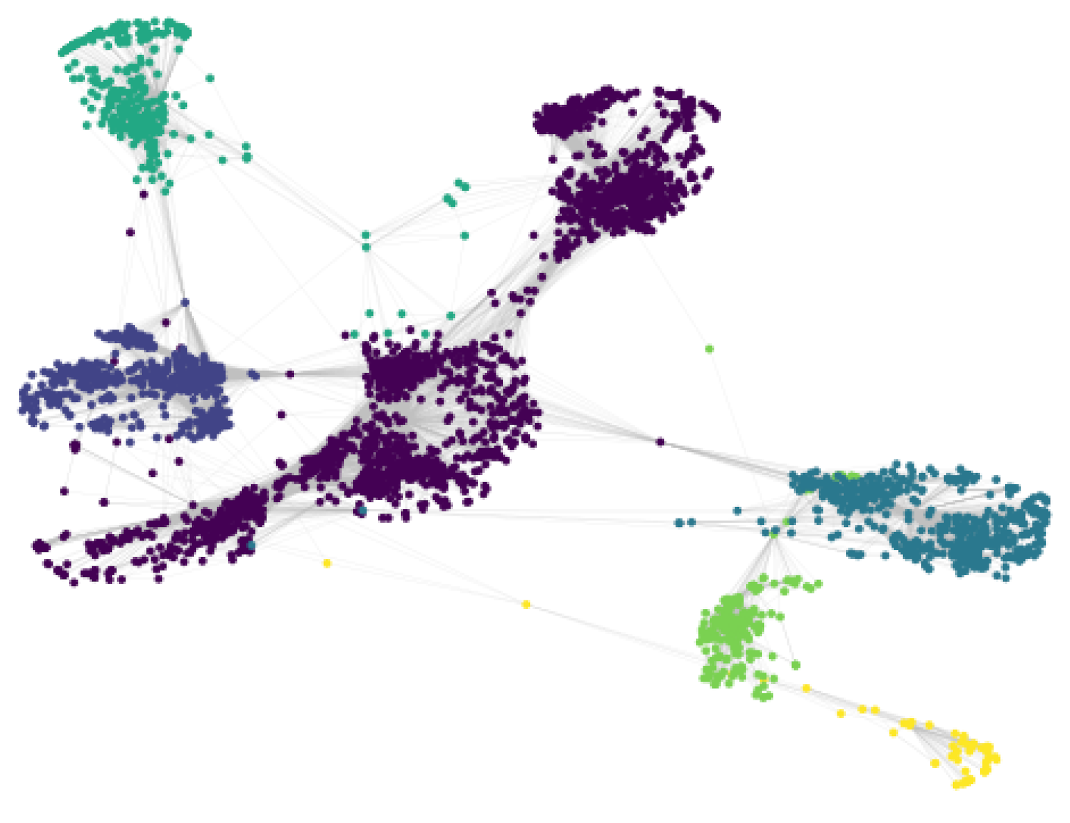
In summary, to partition our graph data sets, we did a pre-analysis to choose parameters where it was needed to obtain the optimal clustering from each algorithm. A visualization of the original graph, and the clusters created by the different algorithms can be seen in Figure 3, Figure 4, Figure 5 and Figure 6. Each cluster is represented with a different color in a gradient style.
6. Results
For our experiments, four actual networks were chosen to evaluate the ranking efficiency and the execution time of the examined method in the case of large networks. Most of the datasets are based on social sites since they consist of numerous nodes and edges. Due to the limitations of our equipment, we selected four graphs that are different in magnitude, to gain more insight. The selected graphs for facebook_combined has 4039 nodes and 88,234 edges [30], the deezer-europe network contains 28,281 nodes and 92,752 edges [31], the soc-gemsec-HU graph has 47,538 nodes and 222,887 edges [32], and the soc-google-plus network has 211,187 nodes and 1,506,896 edges [33]. These networks can be acquired from NetworkRepository [34] and SNAP [35].
To evaluate the efficiency of the examined method, we conducted several experiments with different scenarios on different platforms. As we mentioned earlier, betweenness and closeness centrality was chosen as the focus of the study. We compare the values resulted from these algorithms with the values presented by the investigated method. The execution time of the investigated method and the original centrality measures are also examined. The investigated method used Louvain, Markov, and Paris clustering. We then compared the behavior of centrality measures on subgraphs created by clustering algorithms. The execution time of the investigated method contains both the execution time of the clustering and the centrality measure. The experiments are divided into three parts and are explained below. In the first experiment, we inspected the relation between the top ten nodes selected with no clustering and different clustering methods. In the second experiment, we examined how the algorithms behave compared to plain centrality algorithms when implemented on clusters, using the igraph library [36]. Finally, we looked at how the proposed method performs on a Neo4j graph database using GDS.
6.1. Clusters
Out of the employed clustering algorithms, only the Markov algorithm is not a parameter-free algorithm; before defining the Markov clusters, it was necessary to select the inflation and expansion parameters per graph that produced the highest modularity value. The final parameter values are shown in Table 3.
It can be seen that the Louvain algorithm has the best results, while the other two algorithms have detected a lower density of links inside communities. In Table 4, the number of the clusters created by the different algorithms can be seen.
From the results, it can be seen that the Markov algorithm creates a lot of clusters in the case of every network. Louvain creates considerably fewer clusters; however, the Paris algorithm creates the least cluster.
6.2. Experiment 1: Ranking of the Nodes
In this experiment, we compared the ten most influential nodes extracted by the centrality algorithms without the use of the investigated method and the nodes that were the result of the investigated method. This indicates the node distribution in the clusters. For this experiment we used the facebook_combined (fb), deezer_europe (dz), and soc-gemsec-HU (gm) graphs. The first column shows what rank a node has achieved, based on each algorithm. The first row contains the ranks and the second column shows the result of the basic centrality algorithms. These are followed by the results of the modified version of the algorithms where the Louvain (ln), Markov (mv), and Paris (ps) clustering methods were employed. Table 5, Table 6 and Table 7 show the results of the betweenness (bw) algorithm, while Table 8, Table 9 and Table 10 contain the results of the closeness (cn) algorithm.
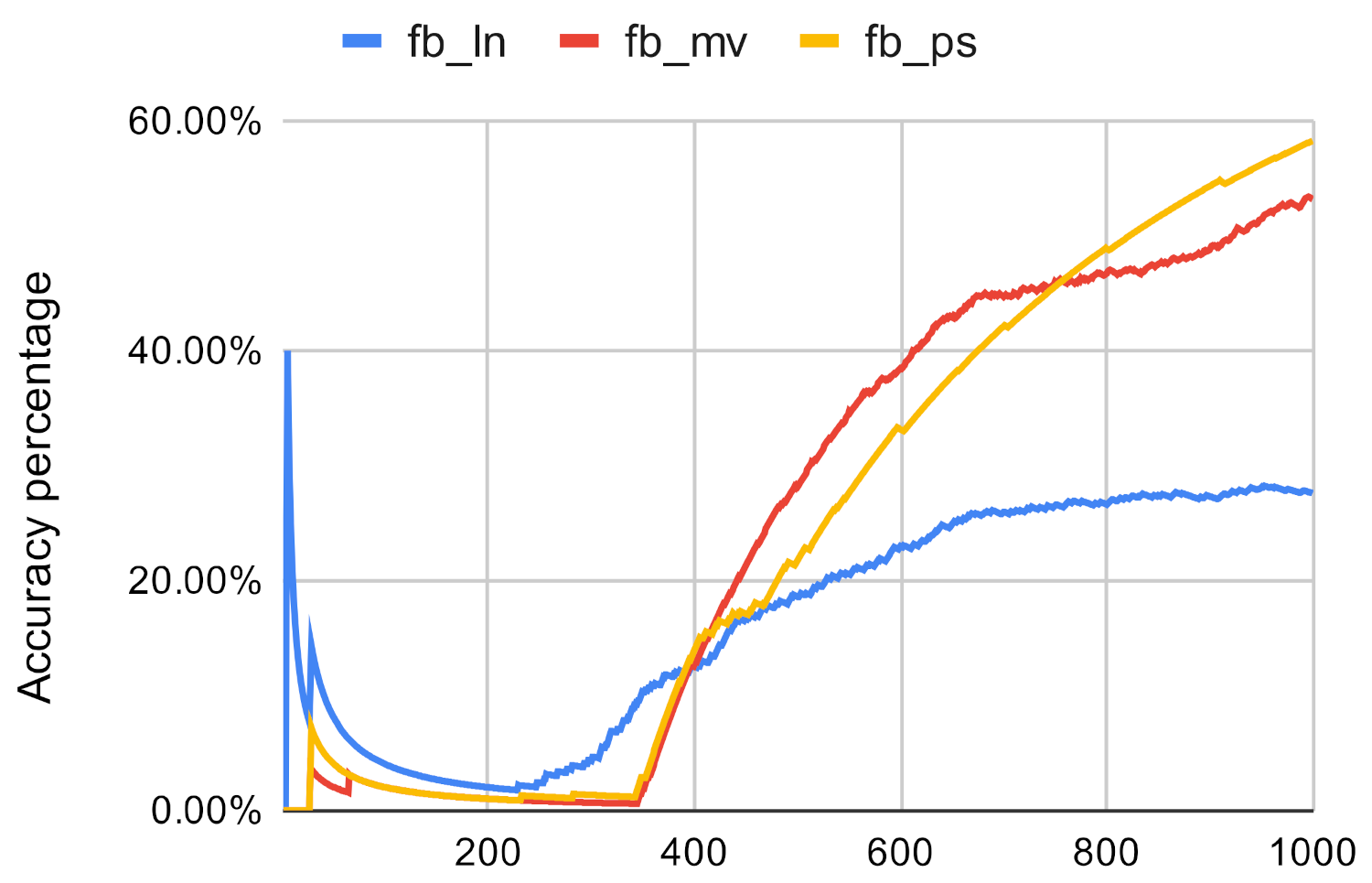
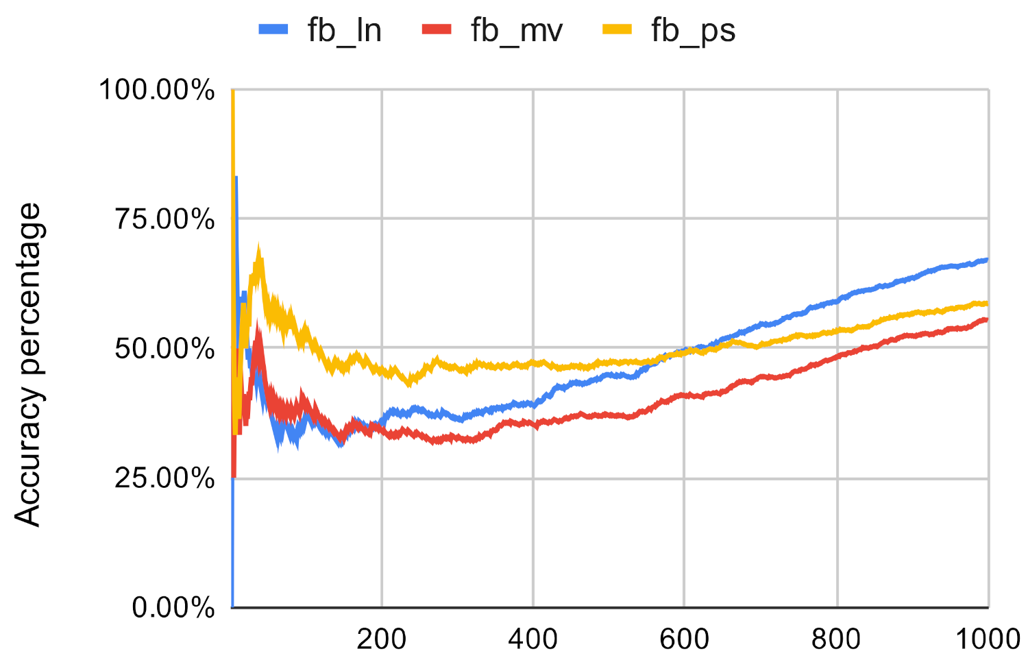
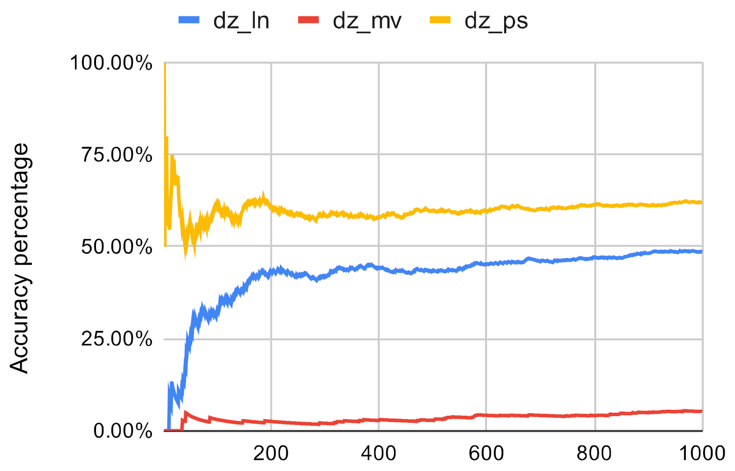
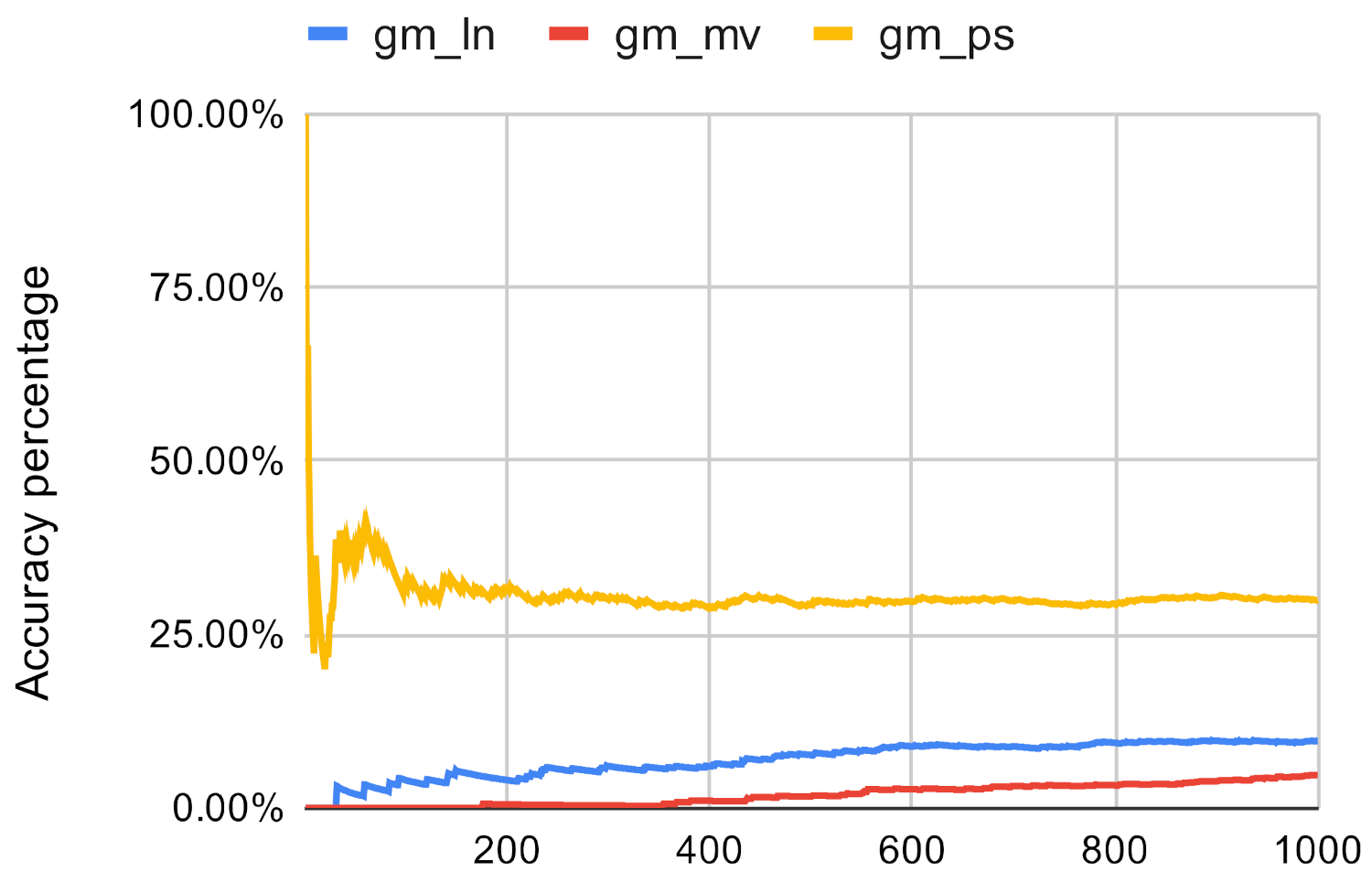
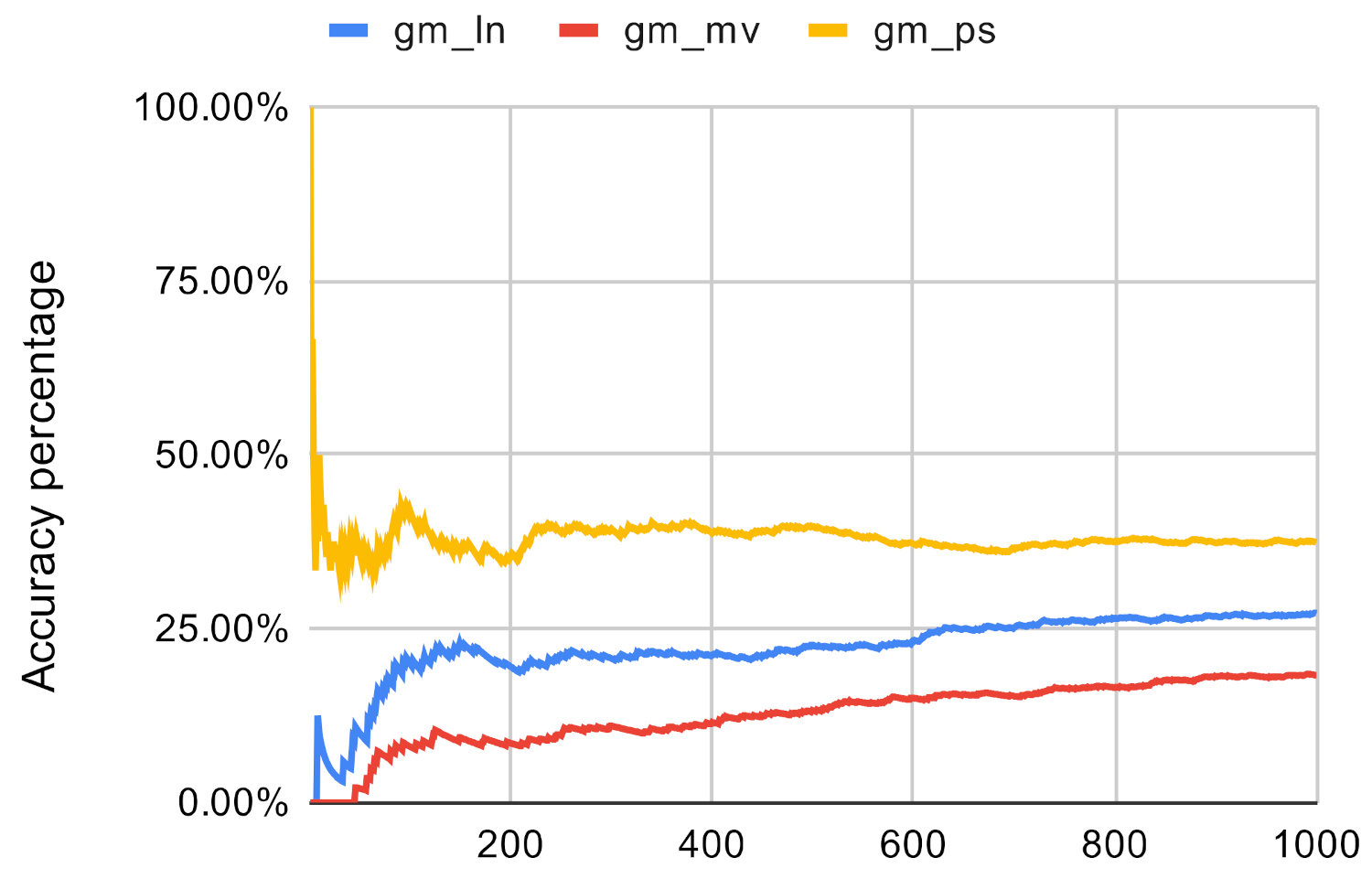
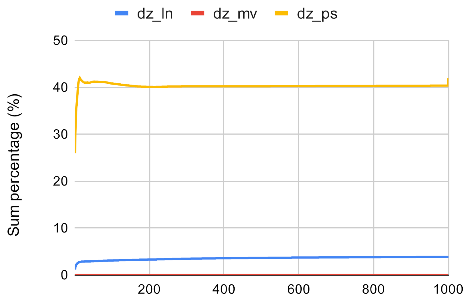
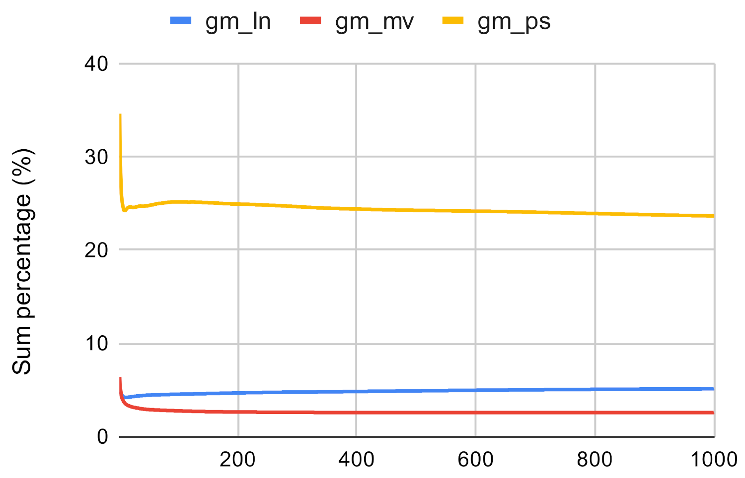
The ranking of the nodes and the similarity between the rankings can be used as an indicator for accuracy. It can be seen that in the case of the used networks, occasionally, the investigated method returns the same nodes as the top 10 nodes as the original centrality measures, however it is not good enough. Because of this, we conducted two more experiments to further evaluate the ranking accuracy of the investigated method. First, we examined that how many nodes of the original methods’ top n ranking could be found in the top n ranking of the investigated method. The results can be seen in Figure 7, Figure 8, Figure 9, Figure 10, Figure 11 and Figure 12. The x axis represents the number of the top nodes that were examined, while the y axis represents the accuracy.
It can be seen that in the case of closeness centrality, the investigated method does not perform well, especially if the network is small in scale. Out of the clustering methods, the Paris clustering has the best accuracy, however, in the best case its only 62.43%. The same could be told about betweenness centrality except that the investigated method is not sensitive to networks size in this scenario.
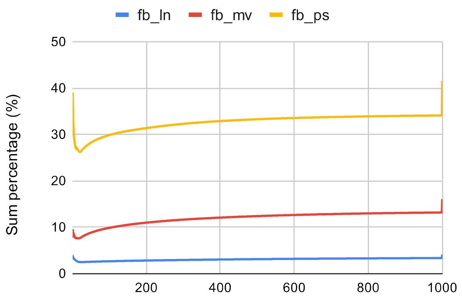
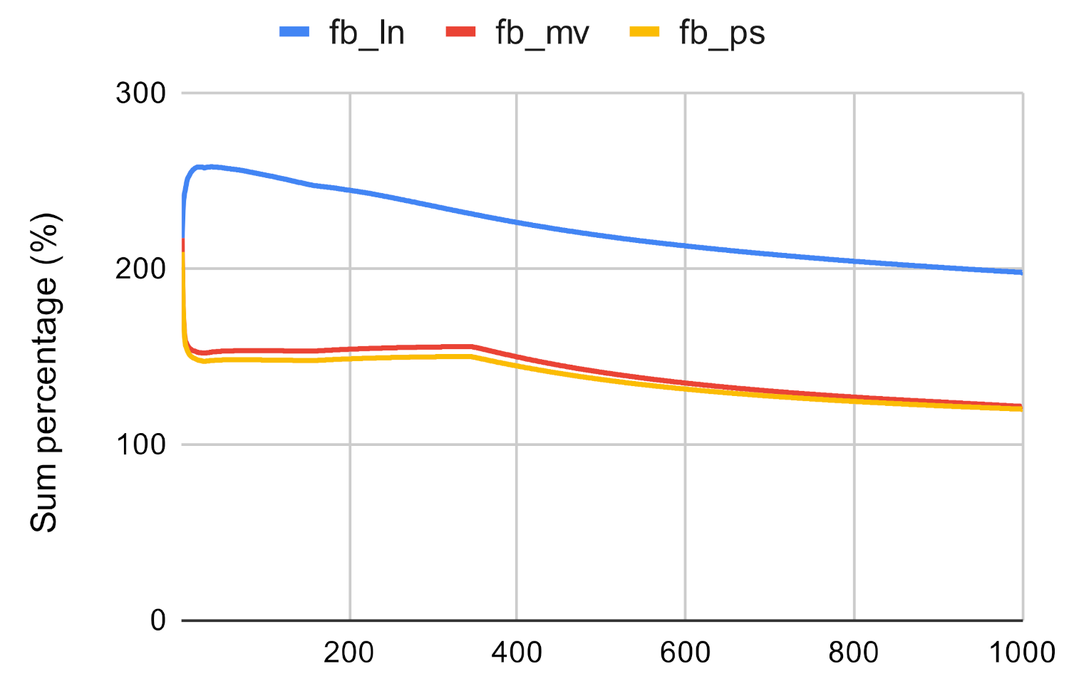
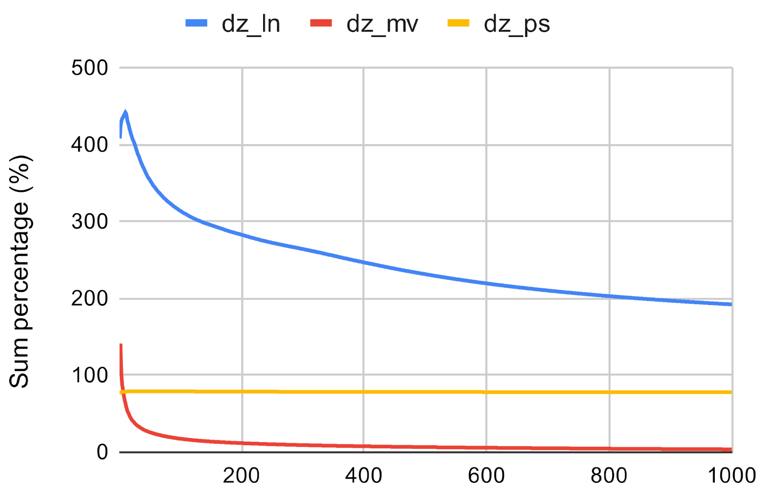
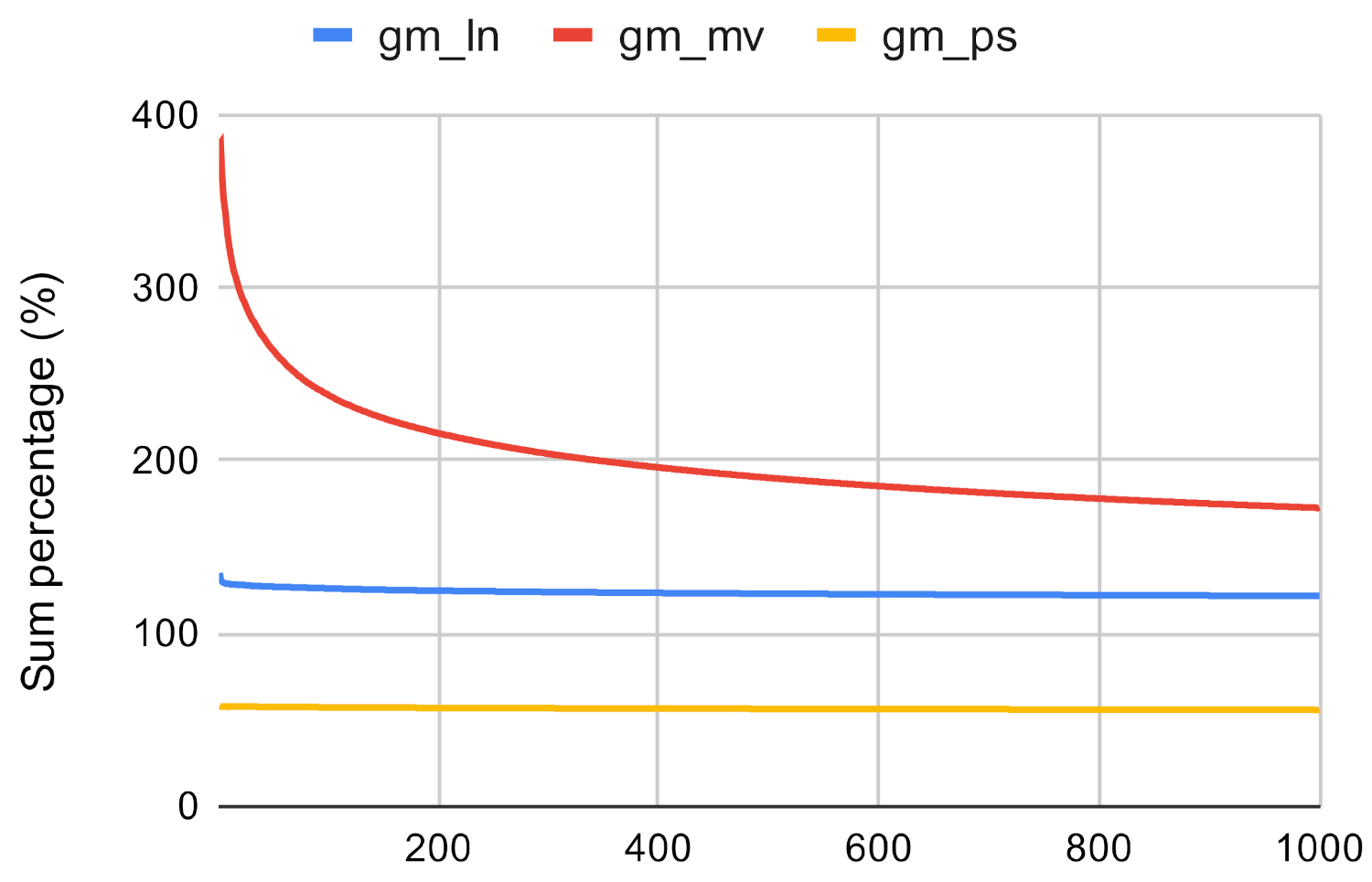
Second, we use the values assigned to the nodes by the centrality measures to examine the accuracy. We compare the sum of the top n value by the original centrality measures and the sum of the top n node values by the investigated method. If the investigated method has a high enough score then it approximates the traditional centrality measures well. Figure 7, Figure 8, Figure 9, Figure 10, Figure 11 and Figure 12 showcases the results of this experiment. The x axis represents the number of the top nodes that were examined, while the y axis represents the accuracy.
Based on Figure 13, Figure 14 and Figure 15 it can be said that the investigated method proves to be not accurate enough if it is used to approximate the result of the betweenness centrality measure. The Paris algorithm has the best result, however, the sum of its top values is only about 25–40% of the sum of the original betweenness values.
On the other hand, Figure 16, Figure 17 and Figure 18 showcase that the investigated methods sum of values is almost always greater than the original methods when it is used with the Louvain clustering algorithm. On average, its sum is 197.73% of the conventional centrality algorithm, which demonstrates that the investigated method is able to approximate the closeness centrality method.
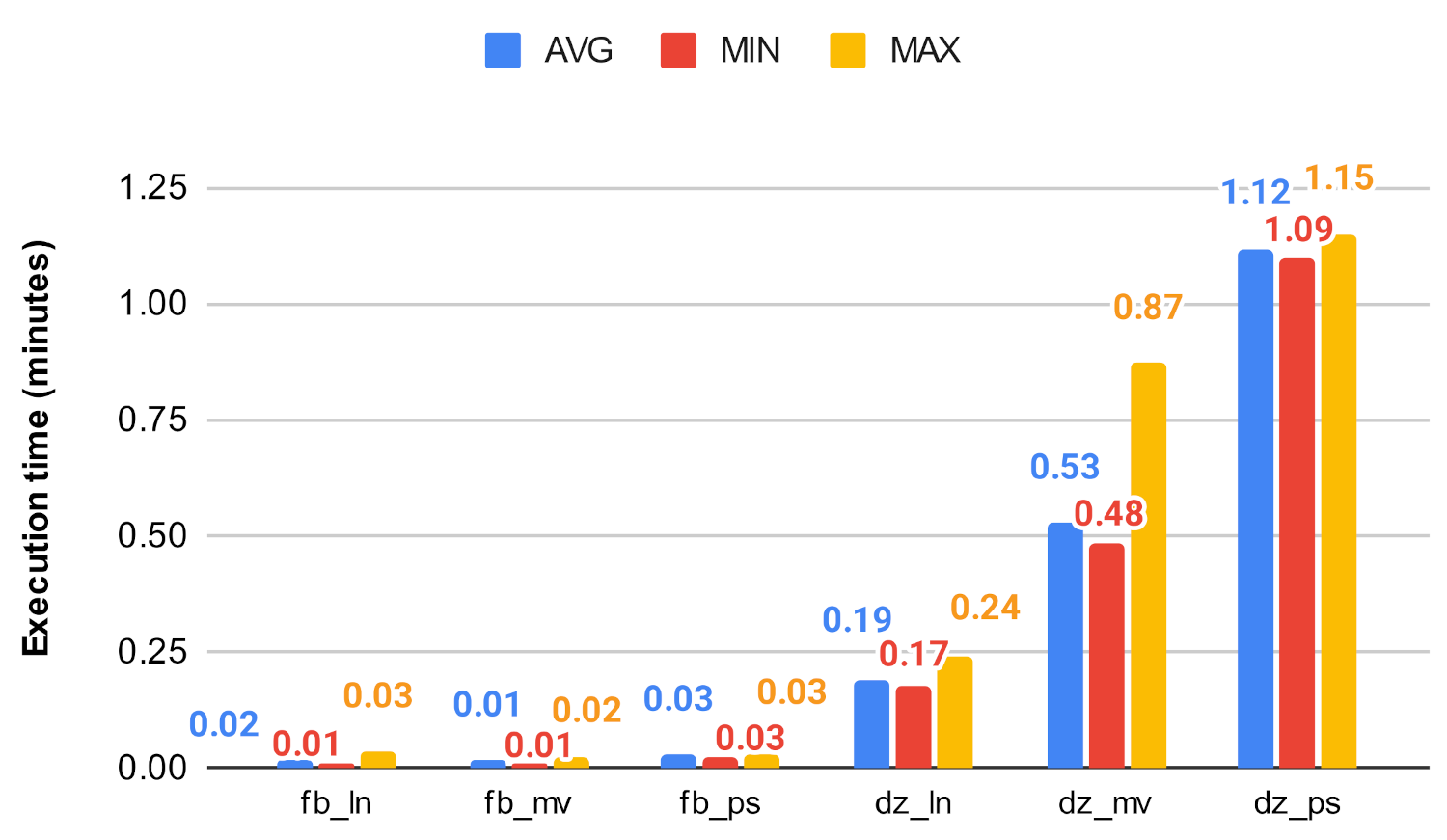
6.3. Experiment 2: Runtime without Graph Database
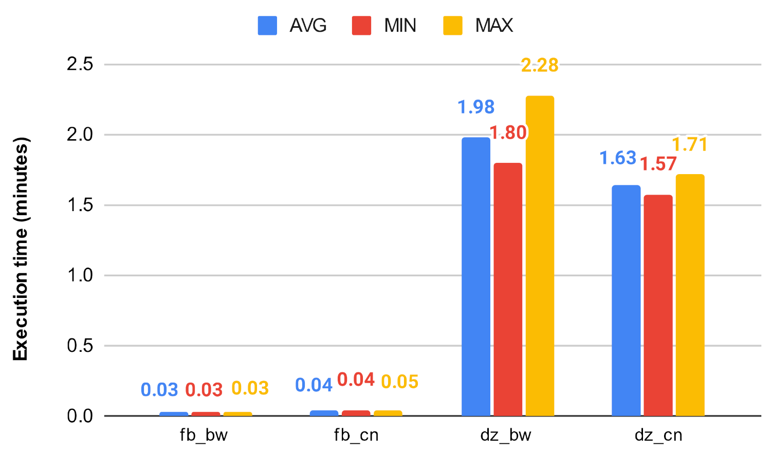
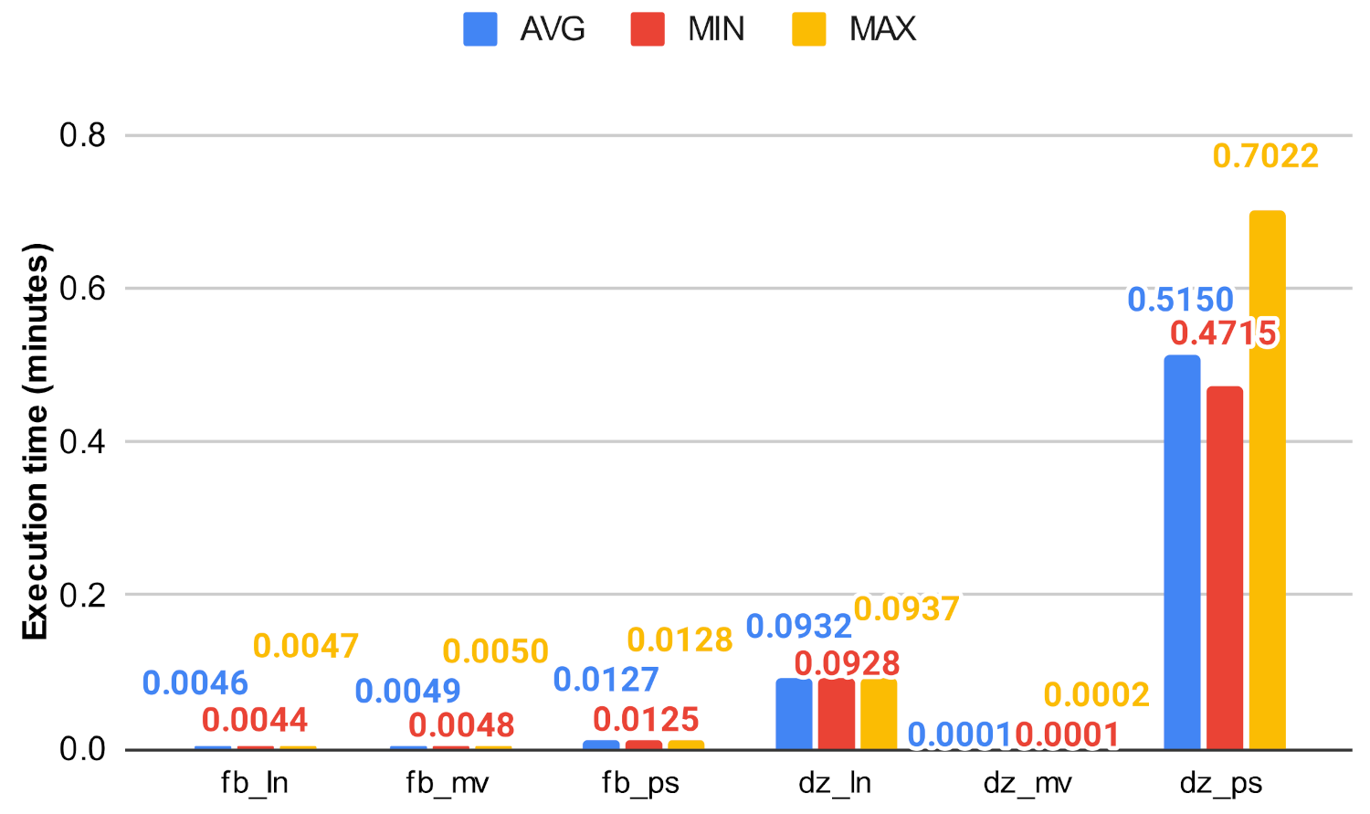
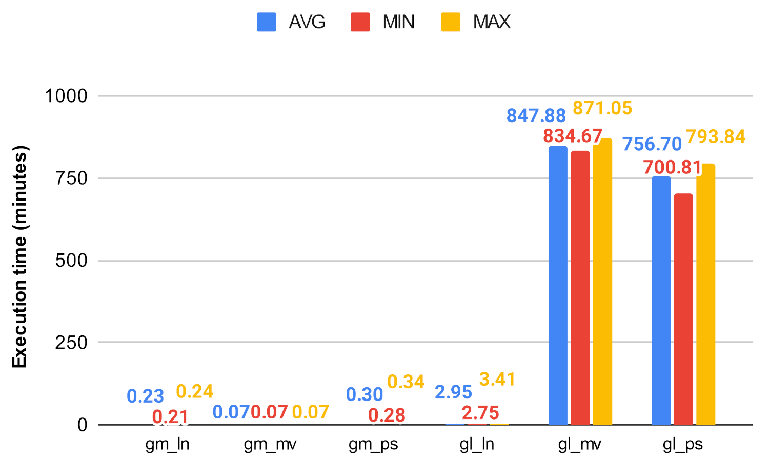
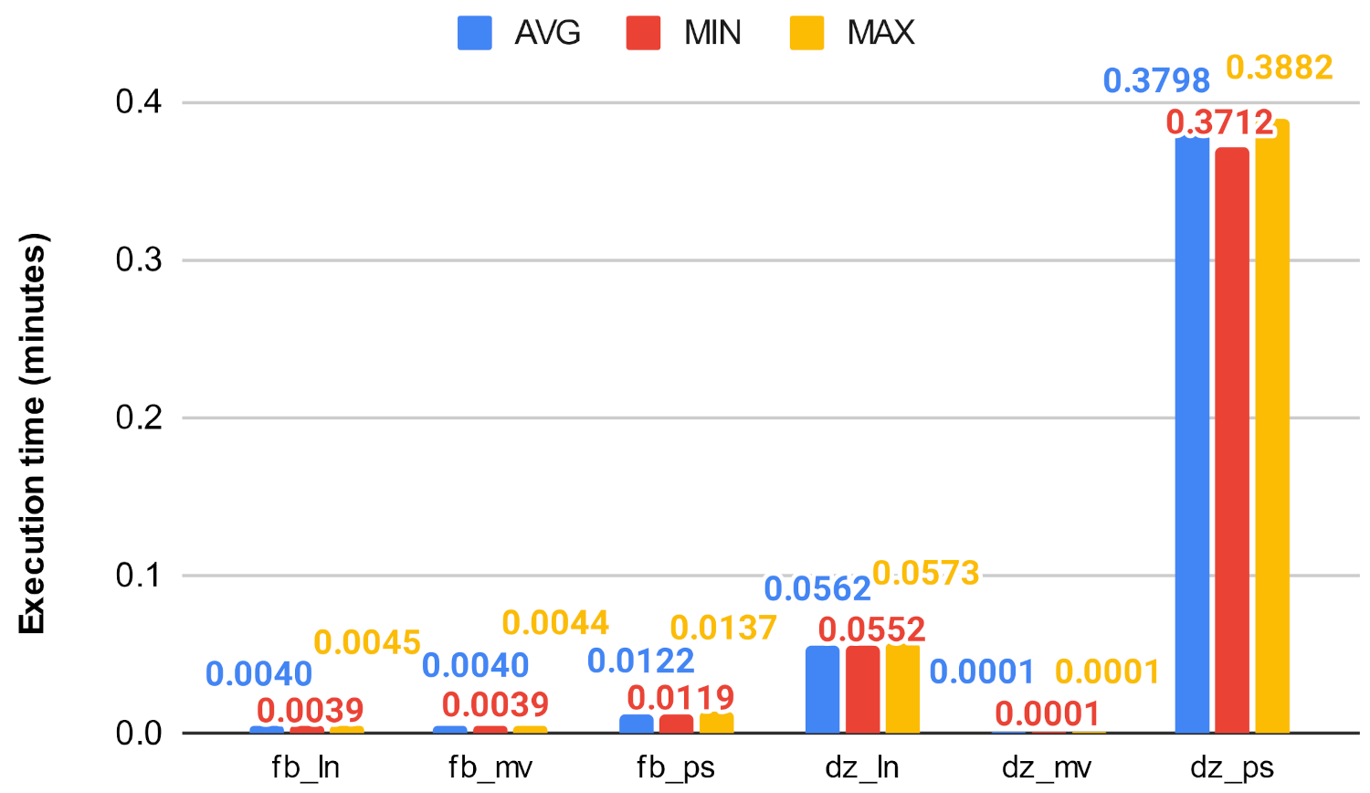
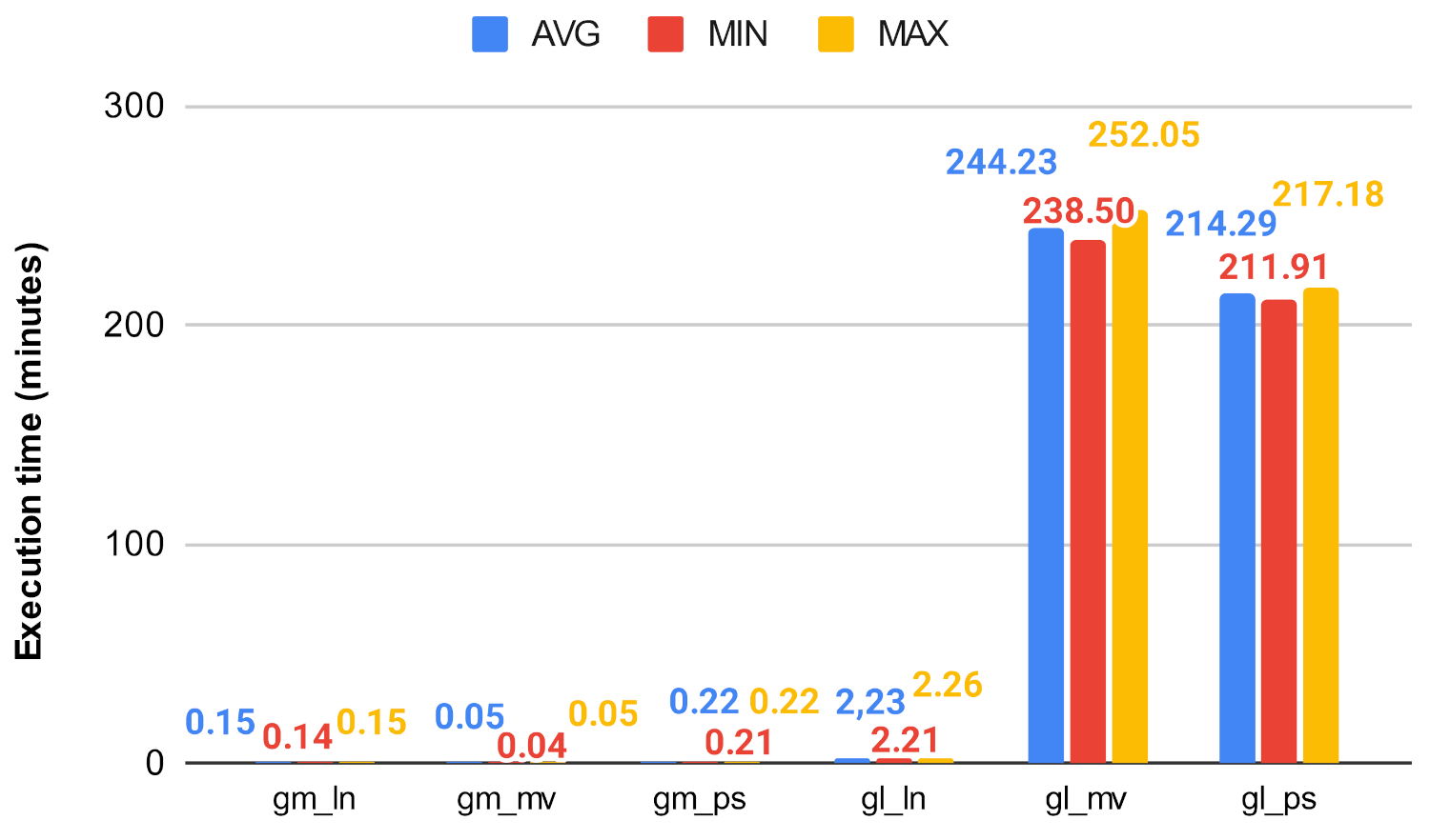
In this experiment, we evaluated the efficiency of the original centrality measures and the investigated algorithm with the use of the execution time they achieved. The algorithms were implemented in Python, using the python-igraph library. Due to the underlying C library, igraph is more performant in terms of CPU time and memory usage than the similar NetworkX library [37] which is a pure-Python implementation. The algorithms were executed 25 times, and the average, minimum, and maximum execution times were taken and are shown Figure 19, Figure 20, Figure 21, Figure 22, Figure 23 and Figure 24. For all of our experiments, we used the same virtual machine with Intel Core CPU (Haswell based) @ 2.40GHz that has 48 cores and 60 GB RAM.
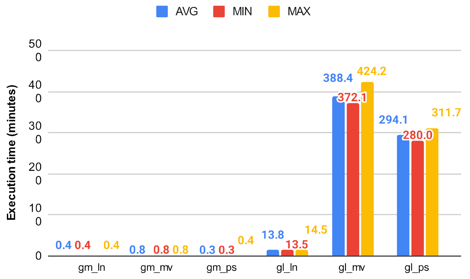
Figure 19 and Figure 20 show how the unmodified centrality algorithms perform on the selected networks. It can be clearly seen that these values are very different, which means that these algorithms do not scale well on large graphs. For example, on the soc-google-plus, the calculation of the betweenness centrality takes an average of 1049.30 min, which is approximately 17.5 h, while closeness on the same graph takes about 4.6 h. Figure 21, Figure 22, Figure 23 and Figure 24 show a decrease in runtime if we run the previous algorithms on the subgraphs that are created based on the clusters. In the case of smaller graphs, it decreases significantly, and in the case of large graphs, a decrease of 12–20% can be observed. Among the clustering algorithms, the number of subgraphs created by Louvain proved to be the most optimal, the Markov method falls behind Louvain, while the Paris clustering is outstandingly worse than the others. The reason behind this is, that the Paris clustering algorithm, as shown in Table 4, has formed a fairly small number of groups, so it is not worthwhile to perform the division with such a low cluster number. In summary, a significant reduction can be achieved in the calculation of centrality values using the igraph library with the incorporation of the Louvain clustering algorithm.
6.4. Experiment 3: Runtime of Graph Database Implementation
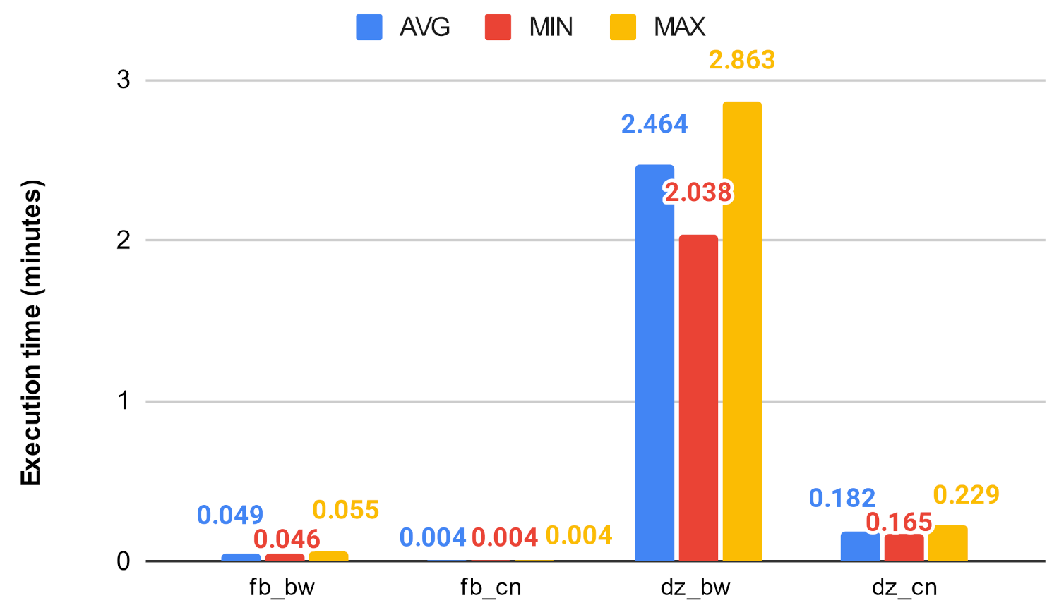
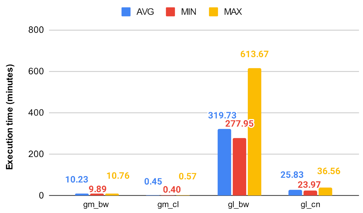
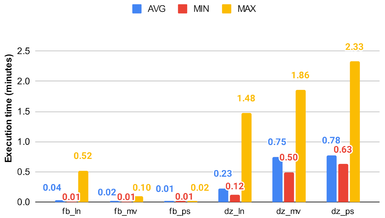
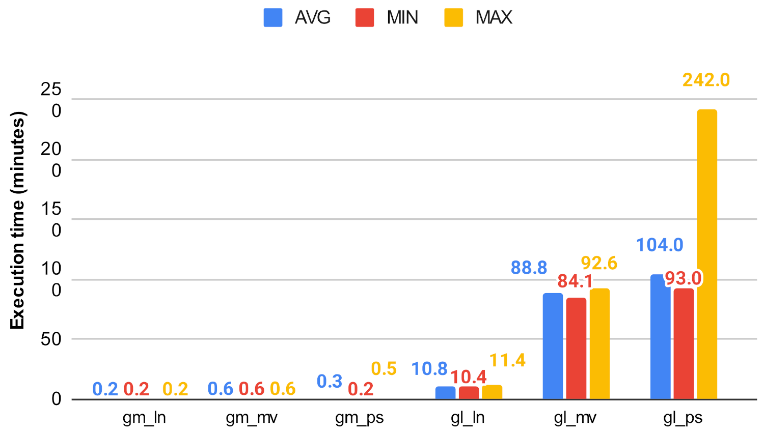
In this scenario, similar to the previous one, the execution time of the algorithm with the use of the Neo4j graph database and the Graph Data Science library with preloaded data was examined. The graph database was used to examine how the method we proposed earlier could be applied, what additional modifications are required, and how much it is supported by the query language of the given database, and what overhead it entails. Furthermore, we wanted to model the situation when the data are already coming from a stored database. We applied the method to graphs that are already available in the database. The library uses multiple CPU cores for graph projections, algorithm computation; however, in our experiments, we used Neo4j Community Edition where the maximum concurrency was limited to 4. The algorithms were executed 25 times, and the average, minimum, and maximum execution times were taken as shown in Figure 25, Figure 26, Figure 27, Figure 28, Figure 29 and Figure 30.
In the GDS environment, the decrease could still be observed in the case of betweenness centrality. This decrease can be seen in Figure 27 and Figure 28, while in the case of closeness it could no longer decrease the execution time of the procedure, and in many cases even deteriorated it. This could be because of the heavy optimization in the implementation in the GDS library. On the large graphs, the Louvain algorithm continued to scale best, while on the smaller ones, the clustering algorithms performed approximately the same. For example, on the soc-google-plus network, the original betweenness centrality took an average of 319 min (approximately 5.3 h), while Louvain clusters reduced this value to an average of only 13.8 min, which means a huge decrease in terms of execution time. During the tests, we monitored the memory usage, which did not exceed 10 GB for the largest graph, so it can be said that on this platform we have the possibility to run these algorithms with a relatively small memory footprint thanks to the graph projection, and with the use of clustering, the execution time can be further reduced.
7. Discussion and Conclusions
In this paper, we investigated the correctness based on the ranking efficiency, and the execition time of a method that uses network clustering to reduce the calculation of betweenness and closeness centrality measures. The method uses graph clustering algorithms, to create clusters based on the graph. These clusters are then used to create subgraphs, which are smaller in magnitude. The centrality measures are then applied to these smaller subgraphs. The investigated method is based on Louvain, Markov, and Paris clustering algorithms. The efficiency of the method was investigated with the use of large social networks, namely facebook_combined, deezer_europe, soc-gemsec-HU, and soc-google-plus. To evaluate the correctness of the method based on the similarity between the top 10 nodes resulted from the investigated method and between the original centrality measures. Our results yielded that the examination of the top 10 nodes is not good enough to correctly evaluate the accuracy of the investigated method. Based on this, we conducted two more experiments. In the first, we used the nodes that are ranked into the top n by the original methods and the investigated method, respectively. The results showed that in this aspect, the investigated method does not perform well, its best results were around 45–60% when it was used with the Paris clustering algorithm. The second experiment, where the sum of the top n was used to classify the accuracy yielded that in the case of the closeness centrality the Louvain clustering method achieved 197.73% of the original closeness centrality, which indicates that in this case, the investigated method approximates the original centrality measure well. To compare the runtime of the investigated method, we applied it in two different environments. One of them was the igraph library’s implementation of the centrality values, while the other was the popular Neo4j Graph Database in pair with the in-memory Graph Data Science library. Based on our experiments, it could be said that the Louvain algorithm was able to create an optimal number of clusters and has the least execution time. and properly approximates the closeness centrality out of the three investigated graph clustering methods. In the case of GDS, we observed that clustering brought improvement only in the calculation of betweenness.
Our paper only considers time consumption, and the similarity between the top 10 nodes for accuracy, and does not consider other indicators such as other types of accuracy. Because of this, in the future, we are planning to perform more experiments to gain more insight into the use of clustering methods. These experiments would evaluate the memory usage, other aspects of accuracy, as well as the complexity of the centrality measures if they are used together with a clustering algorithm.
Author Contributions
Conceptualization, P.M., B.S. and A.K.; methodology, P.M., B.S. and A.K.; software, P.M. and B.S.; validation, P.M., B.S. and A.K.; investigation, P.M., B.S. and A.K.; writing—original draft preparation, P.M., B.S. and A.K.; writing—review and editing, P.M., B.S. and A.K.; supervision, A.K.; project administration, A.K. All authors have read and agreed to the published version of the manuscript.
Funding
The project has been supported by the European Union, co-financed by the European Social Fund (EFOP-3.6.3-VEKOP-16-2017-00002). This research was also supported by grants of “Application Domain Specific Highly Reliable IT Solutions” project that has been implemented with the support provided from the National Research, Development and Innovation Fund of Hungary, financed under the Thematic Excellence Programme TKP2020-NKA-06 (National Challenges Subprogramme) funding scheme.
Institutional Review Board Statement
Not applicable.
Informed Consent Statement
Not applicable.
Data Availability Statement
Publicly available datasets were analyzed in this study. The data can be found on http://networkrepository.com/ and https://snap.stanford.edu/data/ (accessed on 11 February 2021).
Acknowledgments
This publication is the partial result of the Research & Development Operational Programme for the project “Modernisation and Improvement of Technical Infrastructure for Research and Development of J. Selye University in the Fields of Nanotechnology and Intelligent Space”, ITMS 26210120042, co-funded by the European Regional Development Fund.
Conflicts of Interest
The authors declare no conflict of interest.
Abbreviations
The following abbreviations are used in this manuscript:
| bw | Betweenness centrality |
| cn | Closeness centrality |
| ln | Louvian clustering |
| mv | Markov clustering |
| ps | Paris clustering |
| fb | facebook_combined network (4039 nodes, 88,234 edges) |
| dz | deezer-europe network (28,281 nodes, 92,752 edges) |
| gm | soc-gemsec-HU network (47,538 nodes, 222,887 edges) |
| gl | soc-google-plus network (211,187 nodes, 1,506,896 edges) |
| fb_cn | Closeness centrality without clustering on facebook_combined |
| fb_cn_ln | Closeness centrality with Louvain clustering on facebook_combined |
| fb_cn_mv | Closeness centrality with Markov clustering on facebook_combined |
| fb_cn_ps | Closeness centrality with Paris clustering on facebook_combined |
| fb_bw | Betweenness centrality without clustering on facebook_combined |
| fb_bw_ln | Betweenness centrality with Louvain clustering on facebook_combined |
| fb_bw_mv | Betweenness centrality with Markov clustering on facebook_combined |
| fb_bw_ps | Betweenness centrality with Paris clustering on the facebook_combined |
| dz_cn | Closeness centrality without clustering on deezer-europe |
| dz_cn_ln | Closeness centrality with Louvain clustering on deezer-europe |
| dz_cn_mv | Closeness centrality with Markov clustering on deezer-europe |
| dz_cn_ps | Closeness centrality with Paris clustering on deezer-europe |
| dz_bw | Betweenness centrality without clustering on deezer-europe |
| dz_bw_ln | Betweenness centrality with Louvain clustering on deezer-europe |
| dz_bw_mv | Betweenness centrality with Markov clustering on deezer-europe |
| dz_bw_ps | Betweenness centrality with Paris clustering on deezer-europe |
| gm_cn | Closeness centrality without clustering on the soc-gemsec-HU |
| gm_cn_ln | Closeness centrality with Louvain clustering on the soc-gemsec-HU |
| gm_cn_mv | Closeness centrality with Markov clustering on the soc-gemsec-HU |
| gm_cn_ps | Closeness centrality with Paris clustering on the soc-gemsec-HU |
| gm_bw | Betweenness centrality without clustering on the soc-gemsec-HU |
| gm_bw_ln | Betweenness centrality with Louvain clustering on the soc-gemsec-HU |
| gm_bw_mv | Betweenness centrality with Markov clustering on the soc-gemsec-HU |
| gm_bw_ps | Betweenness centrality with Paris clustering on the soc-gemsec-HU |
| ACID | Atomicity, Consistency, Isolation, Durability |
| SNAP | Stanford Network Analysis Project |
| CRUD | Create, Read, Update, Delete |
| GDS | Graph Data Science library |
References
- Pavlopoulos, G.A.; Kontou, P.I.; Pavlopoulou, A.; Bouyioukos, C.; Markou, E.; Bagos, P.G. Bipartite graphs in systems biology and medicine: A survey of methods and applications. GigaScience 2018, 7, giy014. [Google Scholar] [CrossRef] [PubMed]
- Krenn, M.; Häse, F.; Nigam, A.; Friederich, P.; Aspuru-Guzik, A. SELFIES: A robust representation of semantically constrained graphs with an example application in chemistry. arXiv 2019, arXiv:1905.13741. [Google Scholar]
- Deo, N. Graph Theory with Applications to Engineering and Computer Science; Courier Dover Publications: Mineola, NY, USA, 2017. [Google Scholar]
- Khlobystova, A.; Abramov, M.; Tulupyev, A. An approach to estimating of criticality of social engineering attacks traces. In Proceedings of the International Conference on Information Technologies, Saratov, Russia, 7–8 February 2019; pp. 446–456. [Google Scholar]
- Schaab, P.; Beckers, K.; Pape, S. Social engineering defence mechanisms and counteracting training strategies. Inf. Comput. Secur. 2017, 25, 206–222. [Google Scholar] [CrossRef]
- Cuzzocrea, A.; Moscato, V.; Picariello, A.; Sperlí, G. Querying and Learning OSN Graphs for Advanced Viral Marketing Applications. In Proceedings of the 2019 3rd International Conference on Cloud and Big Data Computing, Oxford, UK, 28–30 August 2019; pp. 117–121. [Google Scholar]
- Fensel, D.; Şimşek, U.; Angele, K.; Huaman, E.; Kärle, E.; Panasiuk, O.; Toma, I.; Umbrich, J.; Wahler, A. Knowledge Graphs; Springer: Berlin/Heidelberg, Germany, 2020. [Google Scholar]
- Smidt, H.; Thornton, M.; Ghorbani, R. Smart application development for IoT asset management using graph database modeling and high-availability web services. In Proceedings of the 51st Hawaii International Conference on System Sciences, Hilton Waikoloa Village, HI, USA, 3–6 January 2018. [Google Scholar]
- Chen, H.; Vasardani, M.; Winter, S.; Tomko, M. A graph database model for knowledge extracted from place descriptions. ISPRS Int. J. Geo-Inf. 2018, 7, 221. [Google Scholar] [CrossRef] [Green Version]
- Vela, B.; Cavero, J.M.; Cáceres, P.; Sierra-Alonso, A.; Cuesta, C.E. Using a NoSQL Graph Oriented Database to Store Accessible Transport Routes. In Proceedings of the EDBT/ICDT Workshops, Vienna, Austria, 26 March 2018; pp. 62–66. [Google Scholar]
- Da Silva, W.M.; Wercelens, P.; Walter, M.E.M.; Holanda, M.; Brígido, M. Graph databases in molecular biology. In Proceedings of the Brazilian Symposium on Bioinformatics, Niterói, Brazil, 30 October–1 November 2018; pp. 50–57. [Google Scholar]
- Freeman, L.C. A set of measures of centrality based on betweenness. Sociometry 1977, 40, 35–41. [Google Scholar] [CrossRef]
- Bavelas, A. Communication patterns in task-oriented groups. J. Acoust. Soc. Am. 1950, 22, 725–730. [Google Scholar] [CrossRef]
- Zaki, M.J.; Meira, W. Data Mining and Analysis: Fundamental Concepts and Algorithms; Cambridge University Press: Cambridge, UK, 2014. [Google Scholar]
- Page, L.; Brin, S.; Motwani, R.; Winograd, T. The PageRank Citation Ranking: Bringing Order to the Web; Technical Report; Stanford InfoLab: Stanford, CA, USA, 1999. [Google Scholar]
- Brandes, U. A faster algorithm for betweenness centrality. J. Math. Sociol. 2001, 25, 163–177. [Google Scholar] [CrossRef]
- Shukla, K.; Regunta, S.C.; Tondomker, S.H.; Kothapalli, K. Efficient parallel algorithms for betweenness-and closeness-centrality in dynamic graphs. In Proceedings of the 34th ACM International Conference on Supercomputing, Barcelona, Spain, 29 June 2020; pp. 1–12. [Google Scholar]
- Mendonça, M.R.F.; Barreto, A.M.S.; Ziviani, A. Approximating Network Centrality Measures Using Node Embedding and Machine Learning. IEEE Trans. Netw. Sci. Eng. 2021, 8, 220–230. [Google Scholar] [CrossRef]
- Chou, C.H.; Wang, S.; Shih, H.S.; Sheu, P.C. Scalable Computing of Betweenness Centrality based on Graph Reduction with a Case Study on Breast Cancer Analytics. 2020. Available online: https://www.researchsquare.com/article/rs-72273/v1 (accessed on 20 December 2020).
- Szabari, B.; Kiss, A. Performance evaluation of betweenness centrality using clustering methods. Stud. Univ. Babes-Bolyai Inform. 2020, 65, 59–74. [Google Scholar] [CrossRef]
- Van Dongen, S. Graph Clustering by Flow Simulation. Ph.D. Thesis, University of Utrecht, Utrecht, The Netherlands, 2000. [Google Scholar]
- Azad, A.; Pavlopoulos, G.A.; Ouzounis, C.A.; Kyrpides, N.C.; Buluç, A. HipMCL: A high-performance parallel implementation of the Markov clustering algorithm for large-scale networks. Nucleic Acids Res. 2018, 46, e33. [Google Scholar] [CrossRef] [PubMed] [Green Version]
- Szilágyi, L.; Szilágyi, S.M. Efficient Markov clustering algorithm for protein sequence grouping. In Proceedings of the 2013 35th Annual International Conference of the IEEE Engineering in Medicine and Biology Society (EMBC), Osaka, Japan, 3–7 July 2013; pp. 639–642. [Google Scholar]
- Blondel, V.D.; Guillaume, J.L.; Lambiotte, R.; Lefebvre, E. Fast unfolding of communities in large networks. J. Stat. Mech. Theory Exp. 2008, 2008, P10008. [Google Scholar] [CrossRef] [Green Version]
- Bonald, T.; Charpentier, B.; Galland, A.; Hollocou, A. Hierarchical graph clustering using node pair sampling. arXiv 2018, arXiv:1806.01664. [Google Scholar]
- Newman, M.E.; Girvan, M. Finding and evaluating community structure in networks. Phys. Rev. E 2004, 69, 026113. [Google Scholar] [CrossRef] [PubMed] [Green Version]
- Fortunato, S.; Barthelemy, M. Resolution limit in community detection. Proc. Natl. Acad. Sci. USA 2007, 104, 36–41. [Google Scholar] [CrossRef] [PubMed] [Green Version]
- Neo4j Graph Data Science Library. Available online: https://neo4j.com/docs/graph-data-science/current/ (accessed on 11 February 2021).
- Brohee, S.; Van Helden, J. Evaluation of clustering algorithms for protein-protein interaction networks. BMC Bioinform. 2006, 7, 1–19. [Google Scholar] [CrossRef] [PubMed] [Green Version]
- McAuley, J.J.; Leskovec, J. Learning to discover social circles in ego networks. NIPS 2012, 2012, 548–556. [Google Scholar]
- Rozemberczki, B.; Sarkar, R. Characteristic Functions on Graphs: Birds of a Feather, from Statistical Descriptors to Parametric Models. arXiv 2020, arXiv:cs.LG/2005.07959. [Google Scholar]
- Rozemberczki, B.; Davies, R.; Sarkar, R.; Sutton, C. GEMSEC: Graph Embedding with Self Clustering. In Proceedings of the 2019 IEEE/ACM International Conference on Advances in Social Networks Analysis and Mining 2019, Vancouver, BC, Canada, 27 August 2019; pp. 65–72. [Google Scholar]
- Fire, M.; Tenenboim, R.; Puzis, R.; Lesser, O.; Rokach, L.; Elovici, Y. Computationally Efficient Link Prediction in Variety of Social Networks. ACM Trans. Intell. Syst. Technol. 2013, 5, 10. [Google Scholar] [CrossRef]
- Rossi, R.A.; Ahmed, N.K. The Network Data Repository with Interactive Graph Analytics and Visualization. In Proceedings of the Twenty-Ninth AAAI Conference on Artificial Intelligence, Austin, TX, USA, 25–30 January 2015. [Google Scholar]
- Leskovec, J.; Krevl, A. SNAP Datasets: Stanford Large Network DFataset Collection. 2014. Available online: http://snap.stanford.edu/data (accessed on 11 February 2021).
- Csardi, G.; Nepusz, T. The igraph software package for complex network research. InterJ. Complex Syst. 2006, 1695, 1–9. [Google Scholar]
- Hagberg, A.A.; Schult, D.A.; Swart, P.J. Exploring Network Structure, Dynamics, and Function using NetworkX. In Proceedings of the 7th Python in Science Conference, Pasadena, CA, USA, 21 August 2008; pp. 11–15. [Google Scholar]
Figure 1.
Example of a Markov matrix.

Figure 2.
A property graph: nodes, relationships, and properties.

Figure 3.
Social network: fb-combined.

Figure 4.
Markov clusters on fb network.

Figure 5.
Louvain clusters on fb network.

Figure 6.
Paris clusters on fb network.

Figure 7.
Investigated methods’ accuracy in the case of closeness centrality on fb.

Figure 8.
Investigated methods’ accuracy in the case of betweenness centrality on fb.

Figure 9.
Investigated methods’ accuracy in the case of closeness centrality on dz.

Figure 10.
Investigated methods’ accuracy in the case of betweenness centrality on dz.

Figure 11.
Investigated methods’ accuracy in the case of closeness centrality on gm.

Figure 12.
Investigated methods’ accuracy in the case of betwenness centrality on gm.

Figure 13.
Investigated methods’ sum accuracy in the case of betweenness centrality on fb.

Figure 14.
Investigated methods’ sum accuracy in the case of betweenness centrality on dz.

Figure 15.
Investigated methods’ sum accuracy in the case of betwenness centrality on gm.

Figure 16.
Investigated methods’ sum accuracy in the case of closeness centrality on fb.

Figure 17.
Investigated methods’ sum accuracy in the case of closeness centrality on dz.

Figure 18.
Investigated methods’ sum accuracy in the case of closeness centrality on gm.

Figure 19.
Centrality algorithms’ execution time on fb and dz.

Figure 20.
Centrality algorithms’ execution time on gm and gl.

Figure 21.
Betweenness algorithms’ execution time on fb and dz.

Figure 22.
Betweenness algorithms’ execution time on gm and gl.

Figure 23.
Closeness algorithm’s execution time on fb and dz using ln, mv, and ps.

Figure 24.
Closeness algorithm’s execution time on gm and gl using ln, mv, and ps.

Figure 25.
Centrality algorithms’ execution time on fb and dz.

Figure 26.
Centrality algorithms’ execution time on gm and gl.

Figure 27.
Betweenness algorithms’ execution time on fb and dz.

Figure 28.
Betweenness algorithms’ execution time on gm and gl.

Figure 29.
Closeness algorithm’s execution time on fb and dz using ln, mv, and ps.

Figure 30.
Closeness algorithm’s execution time on gm and gl using ln, mv, and ps.


Table 1.
Modularity for different inflation values.
| Inflation | Modularity |
|---|---|
| 1.5 | 0.8298429 |
| 1.6 | 0.8301530 |
| 1.7 | 0.8302311 |
| 1.8 | 0.8302620 |
| 1.9 | 0.8301715 |
| 2 | 0.8300583 |
| 2.1 | 0.8300583 |
| 2.2 | 0.8300735 |
| 2.3 | 0.8301639 |
| 2.4 | 0.8301789 |
| 2.5 | 0.8301936 |
Table 2.
Modularity for different expansion values.
| Expansion | Modularity |
|---|---|
| 2 | 0.8302620 |
| 3 | 0.8294250 |
| 4 | 0.7876173 |
| 5 | 0.7880002 |
Table 3.
The inflation and expansion parameter choice under the networks.
| Graph | Inflation | Expansion |
|---|---|---|
| facebook_combined | 1.8 | 2 |
| deezer_europe | 1.5 | 3 |
| soc-gemsec-HU | 1.2 | 2 |
| soc-google-plus | 1.1 | 3 |
Table 4.
The number of the clusters created by different clustering algorithms.
| Graph | Louvain | Markov | Paris |
|---|---|---|---|
| facebook_combined | 15 | 10 | 6 |
| deezer_europe | 79 | 773 | 2 |
| soc-gemsec-HU | 24 | 239 | 8 |
| soc-google-plus | 2220 | 1714 | 1706 |
Table 5.
Most influental nodes in facebook_combined network based on betweenness.
| Rank | fb_bw | fb_bw_ln | fb_bw_mv | fb_bw_ps |
|---|---|---|---|---|
| 1 | 107 | 3437 | 107 | 107 |
| 2 | 1684 | 1684 | 698 | 1684 |
| 3 | 3437 | 0 | 1085 | 1577 |
| 4 | 1912 | 1912 | 862 | 698 |
| 5 | 1085 | 107 | 414 | 1718 |
| 6 | 0 | 348 | 686 | 860 |
| 7 | 698 | 414 | 1405 | 348 |
| 8 | 567 | 686 | 0 | 414 |
| 9 | 58 | 483 | 1483 | 1085 |
| 10 | 428 | 1783 | 1465 | 862 |
Table 6.
Most influental nodes in deezer_europe network based on betweenness.
| Rank | dz_bw | dz_bw_ln | dz_bw_mv | dz_bw_ps |
|---|---|---|---|---|
| 1 | 14,771 | 2644 | 1864 | 14,771 |
| 2 | 11,987 | 20,304 | 8413 | 21,925 |
| 3 | 21,925 | 2703 | 5336 | 28,044 |
| 4 | 28,044 | 6536 | 9144 | 11,599 |
| 5 | 4361 | 2961 | 569 | 4361 |
| 6 | 10,971 | 26,754 | 8190 | 3296 |
| 7 | 867 | 14,195 | 2709 | 20,841 |
| 8 | 3296 | 1037 | 23,269 | 23,914 |
| 9 | 23,143 | 15,558 | 6342 | 17,527 |
| 10 | 24,904 | 6371 | 4205 | 867 |
Table 7.
Most influental nodes in soc-gemsec-HU network based on betweenness.
| Rank | gm_bw | gm_bw_ln | gm_bw_mv | gm_bw_ps |
|---|---|---|---|---|
| 1 | 14,900 | 38,301 | 1463 | 14,900 |
| 2 | 40,491 | 46,733 | 42,854 | 24,218 |
| 3 | 24,218 | 36,350 | 45,996 | 35,737 |
| 4 | 14,597 | 5285 | 32,324 | 14,082 |
| 5 | 15,724 | 19,306 | 1912 | 32,622 |
| 6 | 19,081 | 44,985 | 9560 | 14,570 |
| 7 | 7471 | 35,737 | 16,517 | 15,724 |
| 8 | 38,301 | 32,114 | 23,900 | 1397 |
| 9 | 1397 | 6758 | 12,987 | 5772 |
| 10 | 42,899 | 32,582 | 16,952 | 19,081 |
Table 8.
Most influental nodes in facebook_combined network based on closeness.
| Rank | fb_cn | fb_cn_ln | fb_cn_mv | fb_cn_ps |
|---|---|---|---|---|
| 1 | 107 | 584 | 0 | 0 |
| 2 | 58 | 3980 | 56 | 1912 |
| 3 | 428 | 1912 | 67 | 56 |
| 4 | 563 | 107 | 271 | 67 |
| 5 | 1684 | 1684 | 322 | 271 |
| 6 | 171 | 3437 | 25 | 322 |
| 7 | 348 | 0 | 26 | 25 |
| 8 | 483 | 662 | 277 | 26 |
| 9 | 414 | 661 | 252 | 277 |
| 10 | 376 | 659 | 21 | 252 |
Table 9.
Most influental nodes in deezer_europe network based on closeness.
| Rank | dz_cn | dz_cn_ln | dz_cn_mv | dz_cn_ps |
|---|---|---|---|---|
| 1 | 14,771 | 7109 | 9547 | 17,605 |
| 2 | 2518 | 25,373 | 28,219 | 19,721 |
| 3 | 23,143 | 25,105 | 27,457 | 3454 |
| 4 | 24,904 | 25,051 | 25,748 | 17,468 |
| 5 | 867 | 23,819 | 25,360 | 16,782 |
| 6 | 5989 | 20,512 | 24,108 | 13,530 |
| 7 | 20,162 | 17,690 | 20,398 | 20,230 |
| 8 | 10,971 | 15,774 | 20,397 | 11,643 |
| 9 | 21,079 | 10,703 | 19,770 | 418 |
| 10 | 6832 | 10,657 | 14,222 | 5310 |
Table 10.
Most influental nodes in soc-gemsec-HU network based on closeness.
| Rank | gm_cn | gm_cn_ln | gm_cn_mv | gm_cn_ps |
|---|---|---|---|---|
| 1 | 14,900 | 36,365 | 44,157 | 14,900 |
| 2 | 40,491 | 18,432 | 43,794 | 24,218 |
| 3 | 24,218 | 6346 | 40,596 | 35,737 |
| 4 | 38,301 | 10,085 | 20,939 | 14,570 |
| 5 | 15,724 | 17,688 | 21,401 | 23,076 |
| 6 | 14,597 | 46,926 | 24,031 | 32,622 |
| 7 | 19,081 | 6252 | 27,277 | 609 |
| 8 | 42,899 | 21,488 | 25,776 | 15,851 |
| 9 | 7471 | 17,615 | 19,884 | 35,950 |
| 10 | 18,877 | 14,082 | 16,302 | 19,081 |
Publisher’s Note: MDPI stays neutral with regard to jurisdictional claims in published maps and institutional affiliations. |
© 2021 by the authors. Licensee MDPI, Basel, Switzerland. This article is an open access article distributed under the terms and conditions of the Creative Commons Attribution (CC BY) license (https://creativecommons.org/licenses/by/4.0/).
Share and Cite
MDPI and ACS Style
Marjai, P.; Szabari, B.; Kiss, A. An Experimental Study on Centrality Measures Using Clustering. Computers 2021, 10, 115. https://0-doi-org.brum.beds.ac.uk/10.3390/computers10090115
AMA Style
Marjai P, Szabari B, Kiss A. An Experimental Study on Centrality Measures Using Clustering. Computers. 2021; 10(9):115. https://0-doi-org.brum.beds.ac.uk/10.3390/computers10090115
Chicago/Turabian StyleMarjai, Péter, Bence Szabari, and Attila Kiss. 2021. "An Experimental Study on Centrality Measures Using Clustering" Computers 10, no. 9: 115. https://0-doi-org.brum.beds.ac.uk/10.3390/computers10090115
Note that from the first issue of 2016, this journal uses article numbers instead of page numbers. See further details here.