
The Influence of Genetic Algorithms on Learning Possibilities of Artificial Neural Networks


Department of Informatics and Computers, Faculty of Science, University of Ostrava, 30. Dubna 22, 70103 Ostrava, Czech Republic
*
Author to whom correspondence should be addressed.
Computers 2022, 11(5), 70; https://0-doi-org.brum.beds.ac.uk/10.3390/computers11050070
Submission received: 17 March 2022
/
Revised: 7 April 2022
/
Accepted: 19 April 2022
/
Published: 29 April 2022
(This article belongs to the Special Issue Human Understandable Artificial Intelligence)
Abstract
:The presented research study focuses on demonstrating the learning ability of a neural network using a genetic algorithm and finding the most suitable neural network topology for solving a demonstration problem. The network topology is significantly dependent on the level of generalization. More robust topology of a neural network is usually more suitable for particular details in the training set and it loses the ability to abstract general information. Therefore, we often design the network topology by taking into the account the required generalization, rather than the aspect of theoretical calculations. The next part of the article presents research whether a modification of the parameters of the genetic algorithm can achieve optimization and acceleration of the neural network learning process. The function of the neural network and its learning by using the genetic algorithm is demonstrated in a program for solving a computer game. The research focuses mainly on the assessment of the influence of changes in neural networks’ topology and changes in parameters in genetic algorithm on the achieved results and speed of neural network training. The achieved results are statistically presented and compared depending on the network topology and changes in the learning algorithm.
1. Introduction
Genetic Algorithms (GAs) are suitable tools for efficient Neural Network (NN) training with minimal demands on computing power and zero demands on resources in the form of data forming sample training sets.
This paper suggests that changes of genetic algorithm parameters are essential for the quality and time-efficiency of the neural network training process. Furthermore, it is demonstrated that the topology of neural networks has an impact on the quality of the results obtained, and especially on the ability to generalize the problem, i.e., repeatedly solve the problem with new input conditions.
Neural networks and genetic algorithms have been combined in a solution for research problems for a long time. However, such a combination does not necessarily bring better results for the optimization problem. Evolutionary optimization usually takes place in the following areas: determining the appropriate neural network topology for solving a given task, the neural network adaptation itself, and finding the appropriate type of adaptation rule. This study focuses on the adaptation of different types of neural network topology for NN learning, and the main benefit of this research is that the analysis of the experimental results help find the optimal topology and optimal parameters of the genetic algorithm and minimize neural network adaptation time. The entire original project is distributed under the MIT license and its whole modification is described in detail in Section 3 of this article.
We provide an insight into the issue of neural networks and evolutionary techniques in the introduction.
1.1. Neural Networks
Neural networks are structures composed of formal neurons. Neurons are mutually interconnected, and the output of one neuron is the input of one or more neurons. Similarly to a biological neuron, there exist synaptic connections between the axon of one neuron and dendrites of other neurons. The excitation function of a biological neuron is modeled by a positive connection weight between formal neurons and the inhibition function is modeled by negative a weight [1].
We distinguish input neurons, whose state determines the input value of the required function, output neurons, whose state determines the result of the calculation of the required function of the neural network, and hidden neurons in multilayer networks, which transmit and process the information between the input and output neurons.
Synaptic weights of all neural connections represent the neural network configuration and the states of individual neurons determine the state of the neural network. The number of neurons and their interconnection determines the neural network topology. A neural network changes in time. The weights change during neural network adaptation. The state of neurons can also change. The same holds for the topology [1].
When testing suitable neural network topologies, we worked with fixed architectures. This means that an initial topology was selected and it did not change during the adaptation process to prevent organizational changes.
An NN adaptation is a process in which the weights on individual connections between neurons change. In the beginning, the initial configuration of the network is set, usually by inserting random values into the individual weights. The actual adaptation then takes place by changing these values over time. These changes in the weights are called NN learning. For network learning, a training set is usually used, which is composed of so-called training patterns. The patterns are pairs of an input and the desired output. If the network has feedback on which input corresponds to the correct output, we speak of learning with a teacher. If the feedback is the value of the quality of the answer/solution, then it is called classified learning. If we do not have a training set of input/output for a given task and use only the inputs, then this is a type of adaptation called self-organization or also learning without a teacher. The goal of adaptation is to find the values of the weights that allow the network to implement the desired function during its activation [1].
During a network’s activation, computations are performed that change the state of individual neurons from the input values on the input neurons and implement the desired function on the output neurons. The states of individual neurons are updated either sequentially or in parallel. Depending on whether they change their state independently or if the update is centrally controlled, we distinguish between synchronous and asynchronous NNs. Depending on whether all non-input neurons have the same activation function or that different neurons use different activation functions, we distinguish a homogeneous and inhomogeneous NN [1]. Multilayered NNs can be considered as the basis for deep learning. Adaptation of a multilayer network can be made by learning with a teacher, most commonly by backpropagation or backpropagation of error, or by learning without a teacher, for example, using evolutionary algorithms. The biggest problem of these networks is usually determining their topology for solving a given problem. Theoretically, the topology, i.e., in particular how many hidden layers and neurons there should be, should correspond to the complexity of the problem to be solved, especially the structure of the relations they describe [1].
“The main challenge of machine learning is that it must perform well on new, previously unrecognized input data. Not just the ones our model has been trained on. The ability to handle new input well is called generalization” [2].
A network with a small capacity, i.e., a small number of hidden layers and neurons, is not able to see the whole problem, usually getting stuck in some local extremes. On the other hand, a network with a large capacity tends to suffer from so-called overlearning. As in to take over the training patterns, including their errors. In both cases, this leads to a poor generalization of the problem [3].
1.2. Global Optimization Algorithms
Evolutionary algorithms solve problems by procedures that mimic the behavior of living organisms and use mechanisms that are typical for biological evolution, such as selection, reproduction, and mutation. They mimic Darwin’s evolutionary theory of population development, where weaker individuals are culled and die and stronger individuals survive to form the next generation of the population. Each population has a set of individuals and such a set undergoes evolution in each generation. The aim is to modify individuals in each generation so that they improve the characteristics of the whole population [4].
The advantages of using genetic algorithms include flexibility. The concept of an evolutionary algorithm can be modified and adapted to solve the most complex problems that arise and to find a workable solution. The entire population of all possible solutions is taken into the account, meaning that the algorithm is not limited to one particular solution, and it has an unlimited number of solutions. While classical methods present a path to a single best solution, evolutionary algorithms contain and can present several potential solutions to the problem [4]. This algorithm is suitable for problems of many variables where the properties of the interrelationships are so extensive that they are unimaginably complex for a classical solution approach and, thus, intractable by other methods.
Evolutionary algorithms are algorithms that work with random changes in the designed solutions. If a new solution is preferable, it replaces the previous one. They belong to the category of stochastic search algorithms [5].
The general function of an evolutionary algorithm can be described as follows:
- generate the initial population
- the initial population has N individuals, for each individual its configuration is generated completely randomly
- a set of completely random solutions to the problem is obtained;
- the problem is solved by all individuals in a given generation;
- evaluation of each individual in the population;
- selection of parents based on fitness;
- reproduction of offspring to the next generation, application of rules for reproduction, crossover, mutation;
- until a satisfactory solution is found, go back to point 2.
We can see that the whole process completely eliminates recalculating the weights of the NN based on the difference between the expected and achieved solution. In many cases, even the expected solution cannot be defined. We can optimize the problem with a completely unknown function. Alternatively, we can optimize problems where obtaining information for feedback would be too time- and/or cost-consuming.
However, a completely random set of individuals in the first generation might result in the solution stuck at an extreme close to the starting point and the population is unable to evolve further. This shortcoming is usually remedied by generating additional populations with random solutions to the problem, and the population with the best result is then chosen as the initial solution [5].
1.2.1. Natural Selection
In nature, the process of natural selection eliminates individuals unsuitable for a given environment, and in turn, suitable individuals survive and reproduce new generations. However, if we were to prefer only the highest-ranked individuals in reproduction, we would greatly reduce the set of candidates for the optimal solution. Even a candidate with a lower rank can help improve the solution in subsequent generations [5].
1.2.2. Genetic Algorithms
Genetics deal with inheritance and variability of living systems, and studies the variation, divergence, and transmission of species and inheritance traits between parents and offspring. Genotype is a collective term for the complete genetic information of an organism (or cell). It is, therefore, a complete genetic program, whose observable manifestation is a phenotype. A phenotype is a set of all inheritance traits of an individual. It is the (more or less) observable manifestation of the genotype [6].
In organisms such as humans, during reproduction, the two halves of the diploid chromosomes that make up the DNA are joined. Each parent contributes one half. A complete description of the individual is encoded in DNA.
So, we have a whole population of individuals that make up the genotype of that population, and an individual represents the phenotype. The basic function of the genetic algorithm is to select individuals for reproduction in the next generation. The selected individuals then correspond to the chromosome carriers for reproduction. By analogy with genetics, binary sequences of individuals represent chromosomes, with individual positions in the sequence corresponding to genes and specific values corresponding to alleles [6].
Individuals are selected on the basis of a fitness rating or their success in solving the target problem, followed by random selection, where the probability of their selection is proportional to their relative fitness rating. The parents selected for the next generation are crossed. Part of the genetic information of the offspring comes from one of the parents and the remaining part is inherited from the other parent. In the natural environment, errors, corrections, and changes occur when parents’ genetic information is crossed. The genetic algorithm takes this effect of mutation into account. Mutation is important in terms of variability in a population, otherwise, the population risks freezing at some local extreme [6].
A diagram of the genetic algorithm:
- initialization of individuals in the population;
- evaluation of the population;
- until the solution is not sufficient or the termination condition is not met, perform the following:
- perform a natural selection on the parents;
- crossover and generation of offsprings;
- mutation of offsprings;
- evaluation of the population;
- repeat step 3.
2. Related Works
There are countless papers on neural networks and their learning using a genetic algorithm (GA). There are also many similar works that demonstrate the ability of neural network learning to present the playing of some computer games. As a typical example, the OpenAI project [7], is a development environment for developing and creating learning algorithms for neural networks. One of its parts implements the Arcade Learning Environment (ALE) [8] for playing Atari games. This environment has become the de facto reference platform for testing the performance of various, mainly Reinforcement Learning (RL) algorithms. Most works on NNs and GAs focus on comparing the suitability of genetic algorithms and other learning algorithms for particular problem domains. It compares their performance and the time required to train the network to successfully solve the problem. The domains that are suitable for solving by a GA are also solvable by other methods. For example, using Reinforcement Learning algorithms such as Deep-Q Learning, or Actor-critical algorithms (Deep Mind’s AlphaGo) and Evolutionary strategies. It turns out that a GA, which has been known for decades, is competitive to the above RL algorithms and even outperforms them in some tasks. In the paper Deep Neuroevolution: Genetic Algorithms Are a Competitive Alternative for Training Deep Neural Networks for Reinforcement Learning [9], results were presented comparing individual learning algorithms with a GA when solving the task of playing classic arcade Atari games just on the ALE platform. The work [9] showed that a GA not only has lower runtime requirements for teaching a neural network, but also achieves better results than the more time-consuming RL algorithms for some games.
A genetic algorithm for NN training is used in many fields of human activity. We list a few applications. For example, in climatology for modeling global temperature changes [10], for creating a monitoring network to measure the state of groundwater [11], in healthcare for early detection of breast cancer [12], in genetics for operon prediction [13], and in bioinformatics [14]. Among industrial applications belong a management and reservation system for airlines [15], finding the optimal robot path for revising complex structures [16], solving vehicle route planning problems [17], or optimizing and simplifying design in CAD systems [18]. A very common application is teaching the motion of robotic arms and machines, planning processes for the assembly and fitting of printed circuit boards (PCBs) [19], or entire robotic lines in machinery or the automotive industry.
In [20], its authors optimized the network topology of CNN (convolutional neural networks) to improve the model performance. CNN has many hyper-parameters that need to be adjusted for constructing an optimal model that can learn the data patterns efficiently. They focused on the optimization of the feature extraction part of CNN, because this is the most important part of the computational procedure of CNN. This study proposed a method to systematically optimize the parameters for the CNN model by using a genetic algorithm (GA).
Many other studies from the machine learning field show that the combination of neural networks and genetic algorithms is very current. The combination of learning artificial neural networks using hybrid approaches (GA) is very current and is based on many studies. If these techniques are combined well, we can achieve better results than if done separately [21,22,23,24,25,26]. At the present time, methods of artificial neural networks and genetic algorithms are used in all possible scientific fields, from medicine to earth sciences. Their greatest use is in the form of computer applications [27,28,29,30,31,32,33,34].
3. Demonstration of Neural Network Learning Using Genetic Algorithms
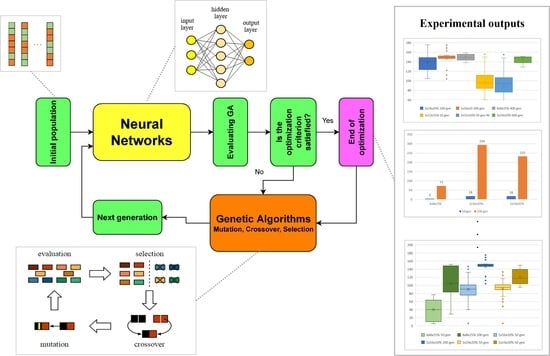
The project creating a visual demonstration of NN learning called SnakeAI by author Greer Viau using a program in Processing [35] shows the topology of an NN and its configuration using a simple diagram of neurons and their connections. The whole project is distributed under an MIT license and is available at: “https://github.com/greerviau/SnakeAI (accessed on 1 April 2022)”. We modified this project without using any frameworks to build the neural network topology and for the learning algorithm. The proposed schematic process flow is shown in Figure 1.
3.1. Game Snake as a Brain of a Neural Network
Snake is an arcade computer game in which the player controls the movements of a snake on a rectangular board. The task is to find food and move so as not to crash into the walls lining the board or into itself. In this case, the game ends. Each time the snake finds food, its body is lengthened, and the player scores a point, which is added to their total score. The theoretical upper limit of the score is limited only by the number of times the snake’s body is extended and the size of the playing area. In fact, it is limited by the player’s ability to react to the placement of new food. Food appears in random locations on the board and it may happen that the snake, due to its body length, will not have access to it.
In the SnakeAI version of the game, the snake can move in four directions, up, down, left, and right on a 40 × 40 square area bounded by outer walls. At the start of the game, the snake has a length of one and the score is zero. With each piece of food found, the body lengthens by one and the score increases by one. The game is programmed to demonstrate NN learning.
Each snake has a brain that is made up of a neural network of several layers. The input layer consists of 24 neurons. The output layer consists of four neurons that control the direction of the snake’s movement (up, down, left, and right). Between the input and output layers, there may be several hidden layers with additional neurons that affect the snake’s abilities. The number of these layers and the number of neurons in them can be modified. For a demonstration, the authors have chosen a topology with two hidden layers of 16 neurons each. In this program, the authors also included the possibility to modify the topology of the snake’s brain using the parameters of the number of hidden layers and the number of neurons in them. The individual neurons are connected to all neurons in the adjacent layer, so it is a so-called fully-connected layer neural network.
During the simulation of the game, the input neurons change colors according to the change of input values, and the output neuron with the highest value is marked in green. This changes the direction in which the snake will move in the next step.
The configuration of the individual connections between neurons is also color-coded. If the connection configuration is negative, it is shown with a red link. If positive, it is shown with a blue link.
3.2. Sensors–Input
The inputs to the input neurons of the network are the values of individual distances to three basic objects of the game in all eight directions (including diagonals). Thus, the distances to the objects along the diagonals are added to the horizontal and vertical distances.
Thus, we can say, with exaggeration, that the snake “sees” the distances to the surrounding objects and recognizes them. The measured distances are:
Distance to walls, to parts of its body and to food.
So, we have three types of objects in eight directions, which equals 24 values to set for the input neurons.
3.3. Fitness
Although the only indicator of success in the snake game is the achieved score, i.e., the number of food objects found, we need a somewhat more detailed evaluation for the development of individuals. Thus, the authors created rules to assess the fitness of each individual. For every step taken in the game where the snake stays alive, the fitness increases by one point, and for every food found, 100 points are added to the fitness. They also set the maximum number of steps a snake can take before it dies to 200. This eliminates the problem that a snake could run around in circles infinitely and therefore reach a higher fitness than a snake that found food. That would not matter much to the game itself, since the overall score is what is evaluated. If a snake finds food, it is given an extra 100 steps to take before it can find more food or die. The maximum number of possible steps is set to 500.
3.4. Evolution
In the original SnakeAI project, each population consists of 2000 individuals. In the first generation, the NN configurations are initialized completely randomly for each individual. The individual knows nothing about the goal of the game, the task to be accomplished, or the rules of the game. The simulation of the game proceeds step by step, where each individual is given the values of the distances to the input neurons (snake. look() method), the potentials of all neurons in the hidden layers are calculated, and the potentials on the output neurons (snake. think()) and the new position of the individual on the board is calculated based on the calculated direction of movement, the output neuron with the largest potential (snake. move()) It is evaluated whether or not it has found food. If yes, the score is increased by one. Conversely whether or not it is in collision with the wall or itself. If it is in collision, it dies and does not participate in the next simulation. These steps are cyclical as long as at least one individual from the whole generation is alive. Once the entire generation dies out, the fitness of each individual in the generation is calculated. The NN configuration of the best individual is copied to the new generation as an individual with an index of zero, and the other individuals in the new generation are generated by NN configurations crossover of the best individuals from the previous generation. When new individuals are reproduced after the crossover, the configurations of their NNs are still changed randomly for 5% of the connections. The mutation ratio can be changed again using the mutation parameter.
3.5. Game Innovation for Measuring the Results
The original project allows to change some basic parameters of the NN topology and the percentage of random mutation of the weights of individuals in the new generation.
A change in the NN topology using these parameters in SnakeAI.pde and their original values:
- int hidden_nodes = 16;
- int hidden_layers = 2;
3.5.1. Change in the Mutation Parameter in the Evolutionary Algorithm
- float mutationRate = 0.05;
It also allows to save the achieved NN configurations to a file for later “replay”.
The program does not provide an indication of its runtime in the original version other than a visual presentation of the runtime of the best individual in a given generation. This is very impractical for testing different setups, and above all, unbearably tedious. The entire SnakeAI project consists of several classes and the SnakeAI.pde program block, which has Processing language methods for setting up the settings() and setup() environments, and a draw() method that is responsible for running the entire program and rendering.
One of the goals of this software upgrade was to make modifications to the program so that neither the classes nor the methods called from SnakeAI.pde had to be changed, making the project backwards compatible with the original program.
For the purposes of our research, the SnakeAI.pde program was modified so that the program measured a certain number of generations, where generations may also contain a number of individuals other than 2000. These measurements or evolutions were made in several iterations, writing the results of all measurements made for a given configuration to a file. The same was done with the NN configuration of the best individual in a given evolution. After measuring a specified number of evolutions, the program stores a summary table of the measured scores for each generation and each evolution of a given topology. It also stores the time taken to compute simulate each evolution and stop. The number of generations in each measurement and the number of individual evolutions (measurements) can be set using new variable parameters:
- int numOfGen = 50;//how many generations will be computed
- int numOfSnakes = 2000;//how many snakes will be in one generation
- int iteration = 20;//how many computations of given topology should be done-evolutions
In order to store the results of each generation in one evolution and the times needed to test one evolution, the following variables were created. Their contents are stored on a disk after completion, both in the table of results for each evolution and in the summary table for all measurements.
3.5.2. Other Modifications of Used Algorithms
Another change in the program code was to disable the simulation of the game progress rendering the best individual in a given generation. The rendering can be turned off by setting a new variable: Boolean showAnimation = false;//false for computing only mode-must be set to true for human play, model show, and original AI computing.
This dramatically speeds up the learning process since there is no need to wait for the best individual of the just-completed generation to display the game progress. The play progress can be visualized after the computation of all evolutions for a given topology and GA parameters are complete, after loading the NN configuration of the best individual of that evolution from the folder of saved results and configurations.
The NN topology, weight connections, color display of the level of each weight, changes to the input layer neurons, and the neuron with the highest potential in the output layer can be newly displayed after the learning process is completed.
All changes were made to preserve the functionality of the original program. That is, if the variable showAnimation is set to true, the program works completely as it was and the new parameters are ignored or do not affect the program’s run.
There is no need to have two environments. One for simulating different topologies and evolutions and measuring the results obtained by them. The other, original environment, for possible visualization of the best individuals of a given evolution. Thus, one can also work with the scenario of training the best individual for a given topology and then visualize and visually compare it with another individual that may have a different NN topology. Thus, we can compare individuals not only based on their scores, but also on the basis of subjective judgments of the chosen strategy for solving the game.
3.6. Changes in the Neural Network Topology
The topology of the considered neural network is influenced by the following parameters:
- int hidden_nodes = 16;
- int hidden_layers = 2.
Rectified Linear Unit activation function (ReLU) is chosen as the activation function. It is defined as the positive part of its Argument (1):
According to [36], in 2017, ReLU was the most used activation function for deep learning neural networks.
In order to compare the results obtained by different topologies, the following topologies were measured.
- topologies with one hidden layer:1 × 4, 1 × 8, 1 × 16, 1 × 24, 1 × 32, and 1 × 48;
- topologies with two hidden layers:2 × 4, 2 × 8, 2 × 16, 3 × 24, 2 × 32, and 2 × 48;
- topologies with three hidden layers:3 × 4, 3 × 8, 3 × 16, 3 × 24, 3 × 32, and 3 × 48;
- and topologies with four hidden layers:4 × 8, 4 × 16.
In total, 20 different NN topologies were compared.
3.7. Changes in the Evolutionary Algortihm
To test the changes at the evolutionary algorithm level, the program was modified so that at the evolutionary level, data could be measured for different numbers of individuals in a generation. Moreover, data could be measured for different levels of mutation. Because of the backward compatibility with the original project and the ability to visualize the best individuals produced, we did not modify the program at the level of assessing the fitness of individuals or changing the rules for the game itself.
Parameters affecting the evolutionary algorithm:
- float mutationRate = 0.05;
- int numOfSnakes = 2000.
The data was measured for populations of 500, 2000, and 4000 individuals per generation and also for different levels of mutation: 5, 10, 15, 20, and 50%.
3.8. Environment to Run Measured Tests
SnakeAI needs the Processing Development Environment [21]. It is an open-source piece of software that is available for Windows, Linux, and Mac OS X. The testing was performed on Windows 10, 64 bit, Processing 3.5.4. Physically, three identical laptops were used for testing with i7-8550U CPU @ 1.99 GHz, four cores, eight logical CPUs. The computation of 60 evolutions, each of the 50 generations of topologies 2 × 32, 2 × 24, 2 × 16, 2 × 8, and 2 × 4 for mutation level 5%, took a total of 98 h of net computation time. In other words, one weekend on all three computers. For this reason, a virtual server was created for the experiment and then run for the actual measurements in multiple instances on the available virtualized infrastructure.
Configuration of the virtualized server environment: Alpine Linux 3.9.3, XFCE Desktop Environment, Processing 3.5.4 for Linux, Image with Virtual Machine (VM) server for VMware ESX version 6.5 environment, OpenJDK 1.8.0_282. Alpine Linux is an Open Source Linux distribution, focused on security, simplicity, and maximum efficiency. However, it retains some convenience and the ability to use the package system to install additional applications.
Tests were run on several VM servers simultaneously. Each server was allocated 3.4 GHz of computational power and four CPUs. All physical servers, where the VM servers were run, had identical CPUs. Thus, conditions were created for the maximum possible objective comparison of the time requirements of different evolutions.
In total, over 4800 evolutions were measured in 80 VM server runs, and the total measurement time exceeded 1620 h, which is 67 days.
Data from all measurements were stored in a central repository and are available when needed. Furthermore, a file was created from this data as an input for a statistical analysis and comparison of the results achieved. Some of the statistical outputs and hypothesis tests used in this work were processed by the JASP program.
4. Analysis of the Achieved Results
The aim of this article is to analyze whether modifications in the genetic algorithm have an effect in order to increase the speed and efficiency of neural network learning. We tested different topologies and different parameters of the evolutionary algorithm in order to compare the changes in the achieved score; both changes leading to its improvement and changes having a negative effect. The original topology set by the authors with two hidden layers, each of 16 neurons, was chosen as the reference test architecture against which the results were compared. There were 2000 individuals in each generation and the chosen mutation rate was 5%. Unless otherwise stated below, for each tested NN topology with different GA parameters, 60 measurements (evolutions, iterations) were performed with 50 generations in each iteration. Each generation had 2000 individuals, the same as the reference one. The measured results for each topology and GA parameters are available at: “https://github.com/josefczyz/snakeAIstatistics (accessed on 1 April 2022)”.
Each of the data folders also contained a Snakes folder, which stores the NN configurations of the best individuals after a given evolution. These configurations can be uploaded back into the program to view the behavior of the trained individual under the new conditions. The placement of food, i.e., the goal and reward in the game, is random each time. This means that a trained individual may not always achieve the same result as in the environment in which it was trained. In addition, each of the data folders contained an EvolutionScores folder, which contained files containing the results achieved by each measured evolution. Each file contains data for each generation of that evolution and the total time required to compute that evolution.
4.1. Comparison of Neural Networks Topologies
4.1.1. Influence of the Number of Hidden Layers
A comparison of the influence of the number of hidden layers can be seen in Table 1. First, a comparison with the reference architecture of 16 neurons in each layer.
The graph in Figure 2 shows the improvement of the result when using only one hidden layer instead of the original two and the deterioration when further increasing the number of inner layers to three. However, with the improvement, there was a noticeable increase in the time required to run all measurements from 11 to 17 h.
4.1.2. Influence of the Number of Neurons in Hidden Layers
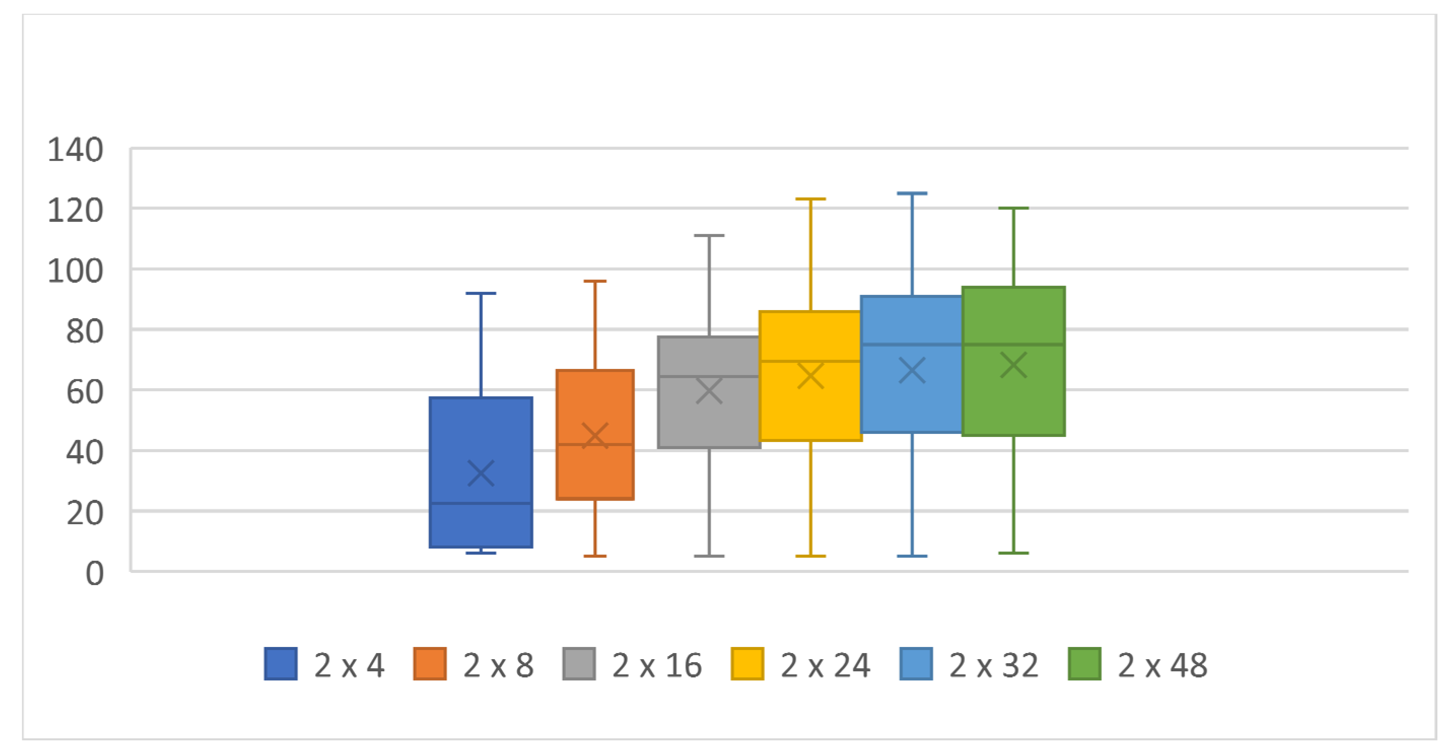
Next, the effect of the number of neurons in each layer was compared with the original design with two hidden layers of neurons. Table 2 and the graphs in Figure 3, Figure 4 and Figure 5 below show that the performance decreases with fewer neurons in the hidden layers and that increasing the number of neurons above 16 resulted in a certain improvement, especially in the increase in maximum score, but the 2 × 24, 2 × 32, and 2 × 48 topologies were no longer different in terms of performance. Noticeable is the increase in the total computation time required for the 2 × 48 topology compared with that of 2 × 32, although both topologies achieved virtually the same results and the snake with the 2 × 32 topology also achieved the maximum score.
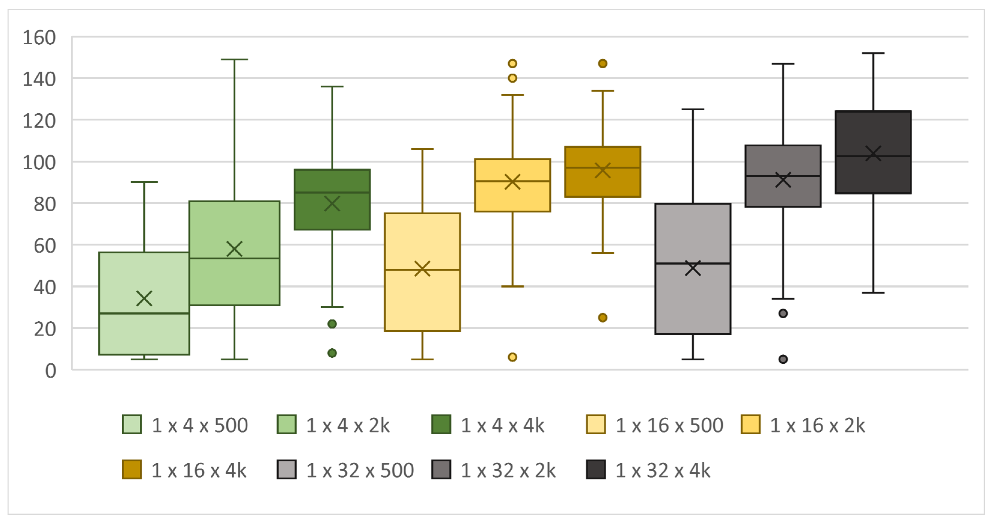
For the topology with one hidden layer, we observe a performance increase in all configurations with neuron counts from 4 to 48 compared with the topology with two hidden layers. The highest score was achieved by the snake with the 1 × 16 topology and again, there were no major differences between the 1 × 16–1 × 48 topologies.
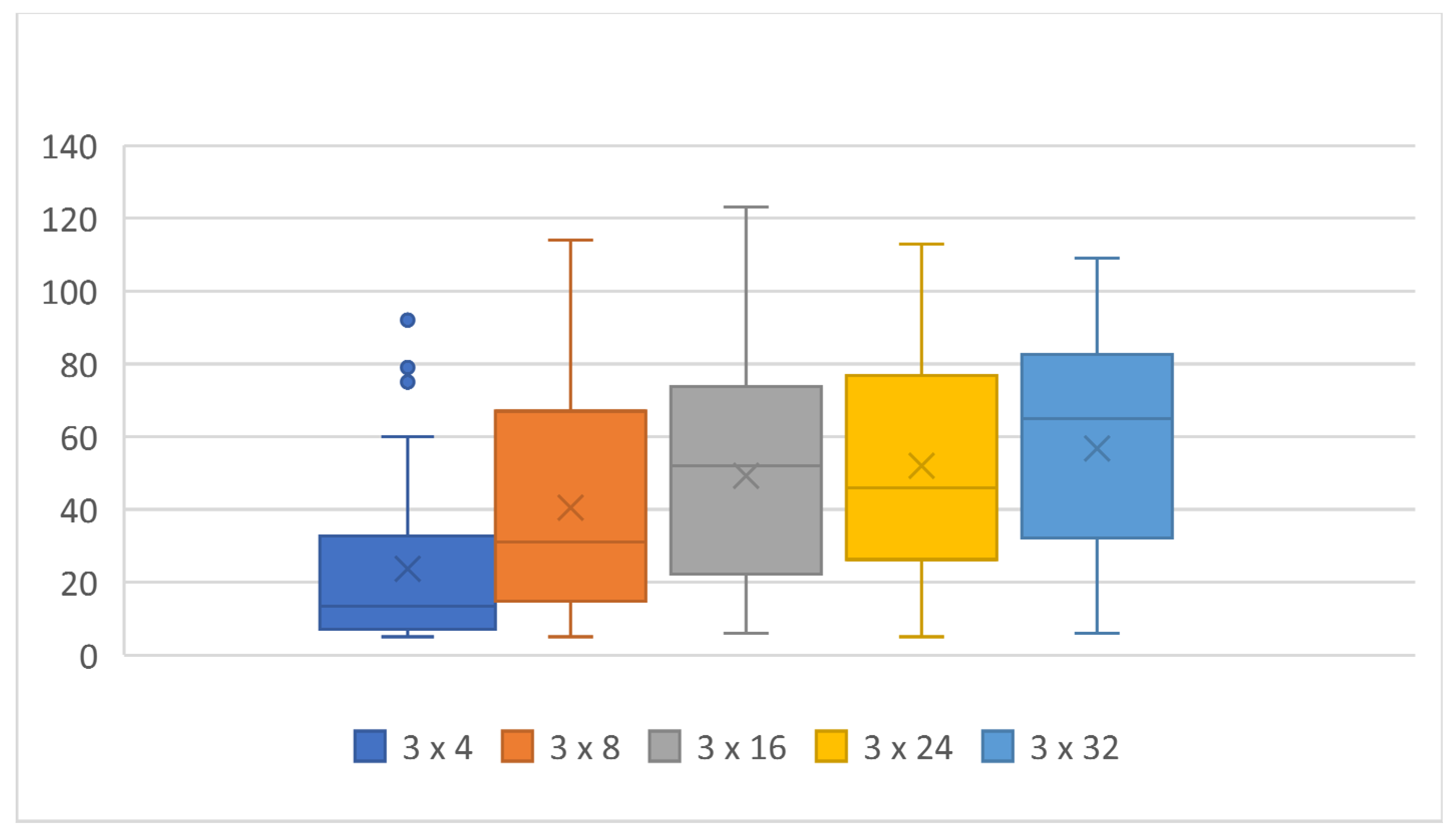
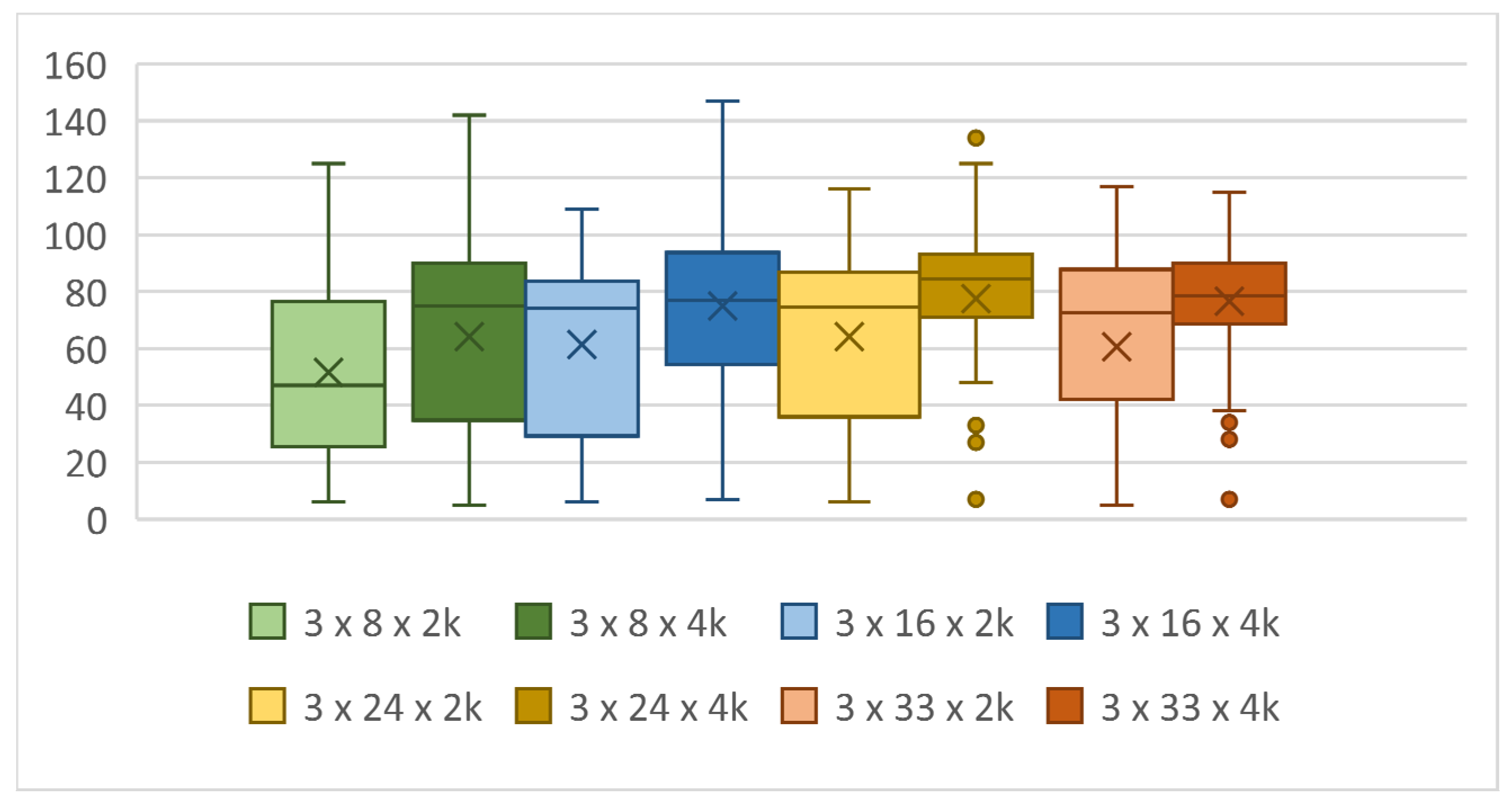
When we tested for changes in the number of neurons in topologies with three hidden layers, we saw a decrease in both the maximum score and the median across the number of neurons compared with the topologies with one and two hidden layers. The computation time also decreased, proportionally to the score achieved.
We tested the effect of the number of layers on the achieved scores in more detail for the 1 × 16, 2 × 16, and 3 × 16 topologies using an ANOVA test.
Since the data were not from a normal distribution, see Table 3—Kruskal–Wallis Test and p < 0.001, the test used is Dunn’s post hoc comparison test, which can be seen in Table 4.
The tests revealed that for each combination of topologies, we must reject the hypothesis that these topologies achieve the same results. p < 0.05 (Holm test pholm, Bonferroni test pbonf) in all comparisons, albeit for the 2 × 16 to 3 × 16 combination closely. Only for the Bonferroni test, the comparison of 1 × 16 and 2 × 16 came to a conclusion that these topologies do not differ; similarly to the 2 × 16 and 3 × 16 topologies. However, there was also a significant difference between the 1 × 16 and 3 × 16 topologies for the Bonferroni test (where z, Wi, Wj are Bonferroni test parameters).
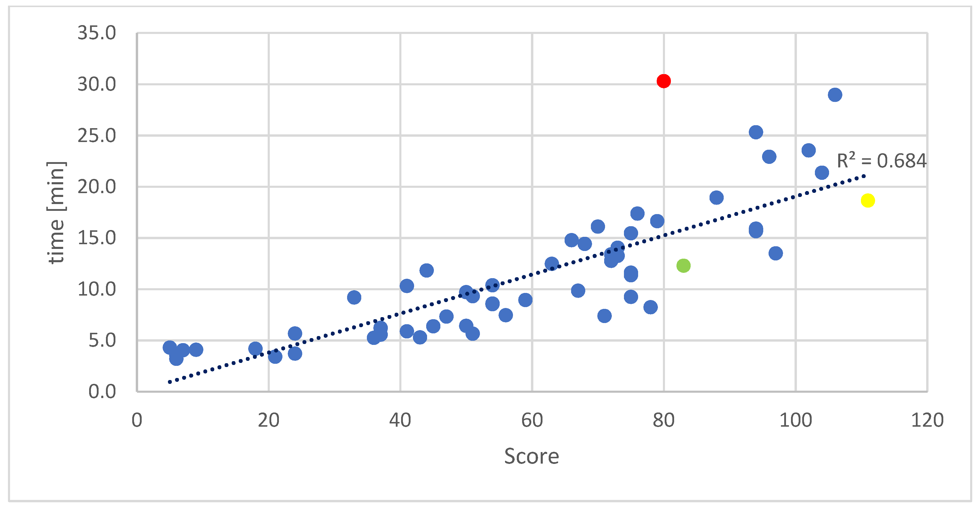
From the score Table 1, Table 2, Table 3 and Table 4 for each topology, we can observe an increase in the computation time as a function of the score. See Figure 6 showing the time required in minutes to compute the score of 60 evolutions, each of 50 generations, where there were 2000 individuals in each generation for the 2 × 16 topology. Individuals that are able to achieve high scores in early generations are marked in red, green and yellow.
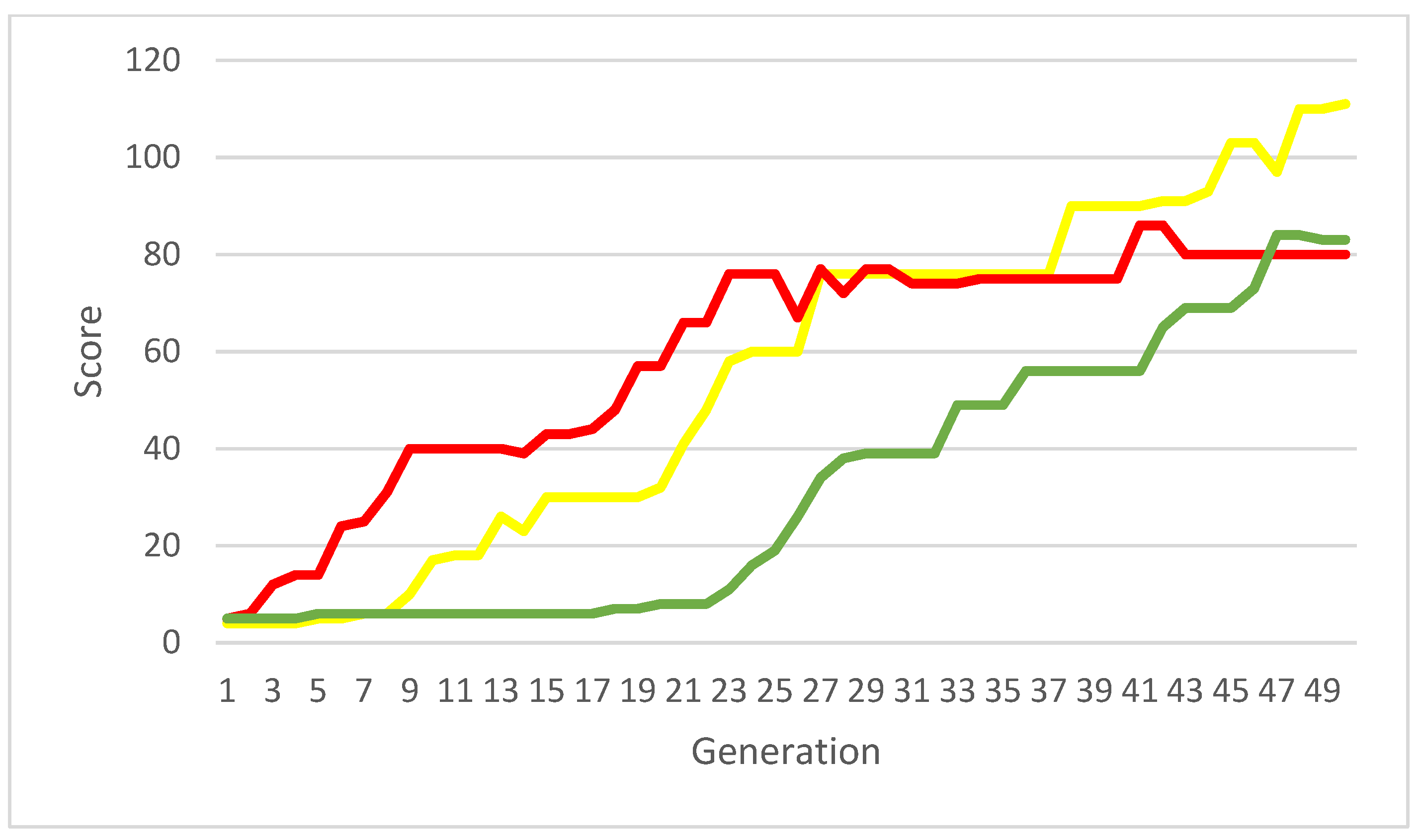
The running time of one evolution was linearly dependent on the score. Obviously, as the total score increased, the computation time also increased. Looking closely at the measurements of the evolutions in Figure 7, marked in red, green, and yellow, one can see that the total time of one measurement depended on how early (in which generation) individuals were able to achieve a high score. In other words, simulating the play of successful individuals (from Figure 6) that achieve higher scores in an early generation was more time-consuming.
The colors correspond to the uniform measurements in the previous graph. The total running time for the evolution that achieved a high score of 40 already in the nineth generation was more than twice as long as the evolution that reached the same score only in the 29th generation, and the total scores of the two evolutions in the 50th generation were almost identical 80 and 83, respectively. The evolution that reached a maximum score of 111 and whose score increase was almost linear across generations took only about two thirds of the computation time of the most time-consuming and less successful evolution.
While comparing topologies 1 × 4, 1 × 8, and 1 × 16, we observed an improvement and an increase in the score, hence changes in the number of neurons had an effect on the scores achieved.
Comparing further topologies 1 × 16, 1 × 24, and 1 × 32, we can say that the change in the topology towards a higher number of neurons in the hidden layer does not statistically affect the score achieved.
4.2. Comparison of Changes in the Evolutionary and Genetic Algorithm
Parameters that have a direct influence on the evolutionary algorithm are the percentage of mutation, the number of individuals in a generation, and the number of generations after which we terminate the evolutionary process and calculate the NN configuration. The genetic algorithm could also be influenced by other factors, such as the method of calculating the fitness of an individual or the method and parameters for selecting individuals for a crossover.
4.2.1. Influence of Individuals in a Generation
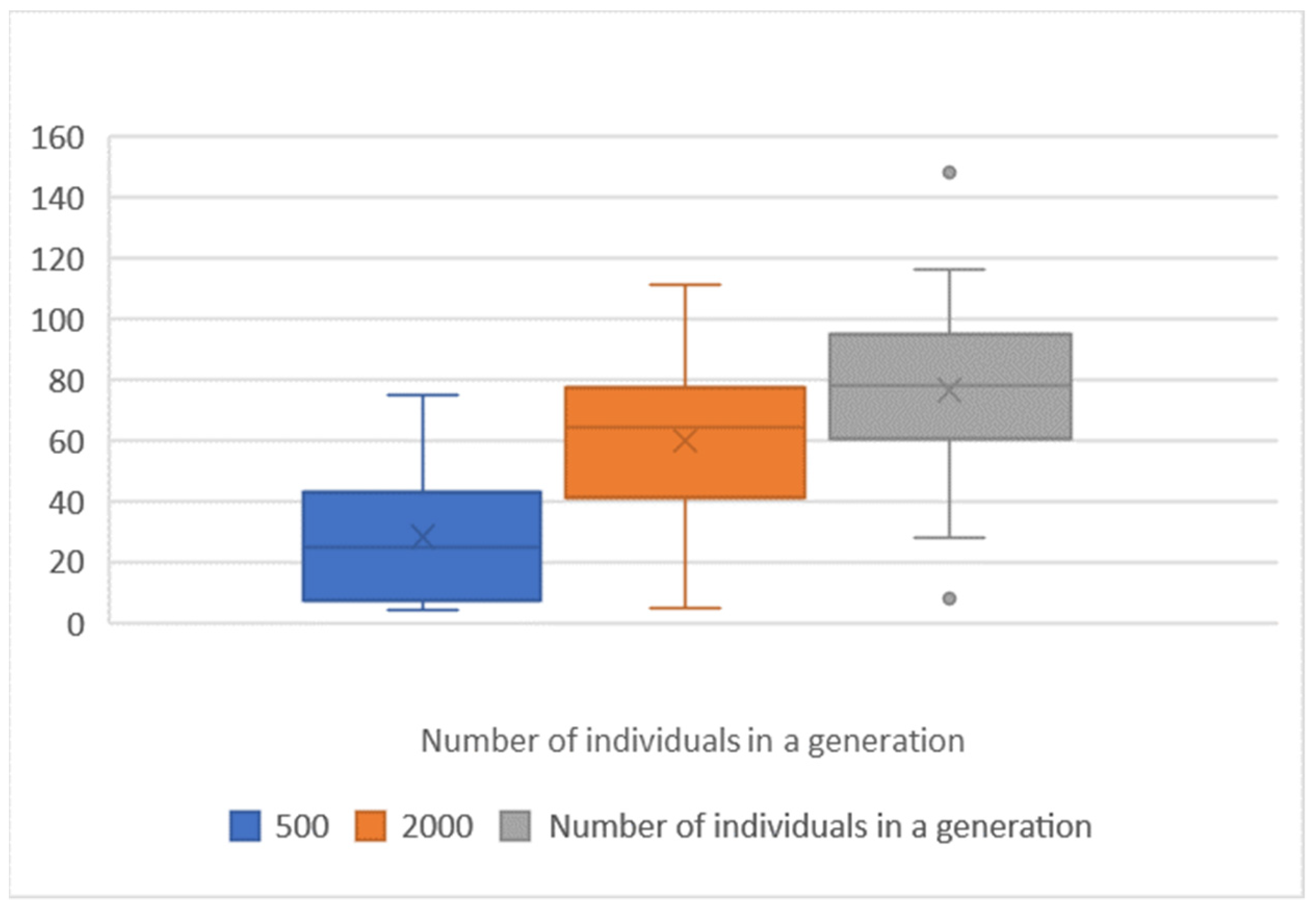
First, the effect of the number of individuals in the population on the score. A comparison of the results with 500 and 4000 individuals in a generation with the reference topology 2 × 16 with 2000 individuals in a generation and a 5% mutation is provided in Table 5.
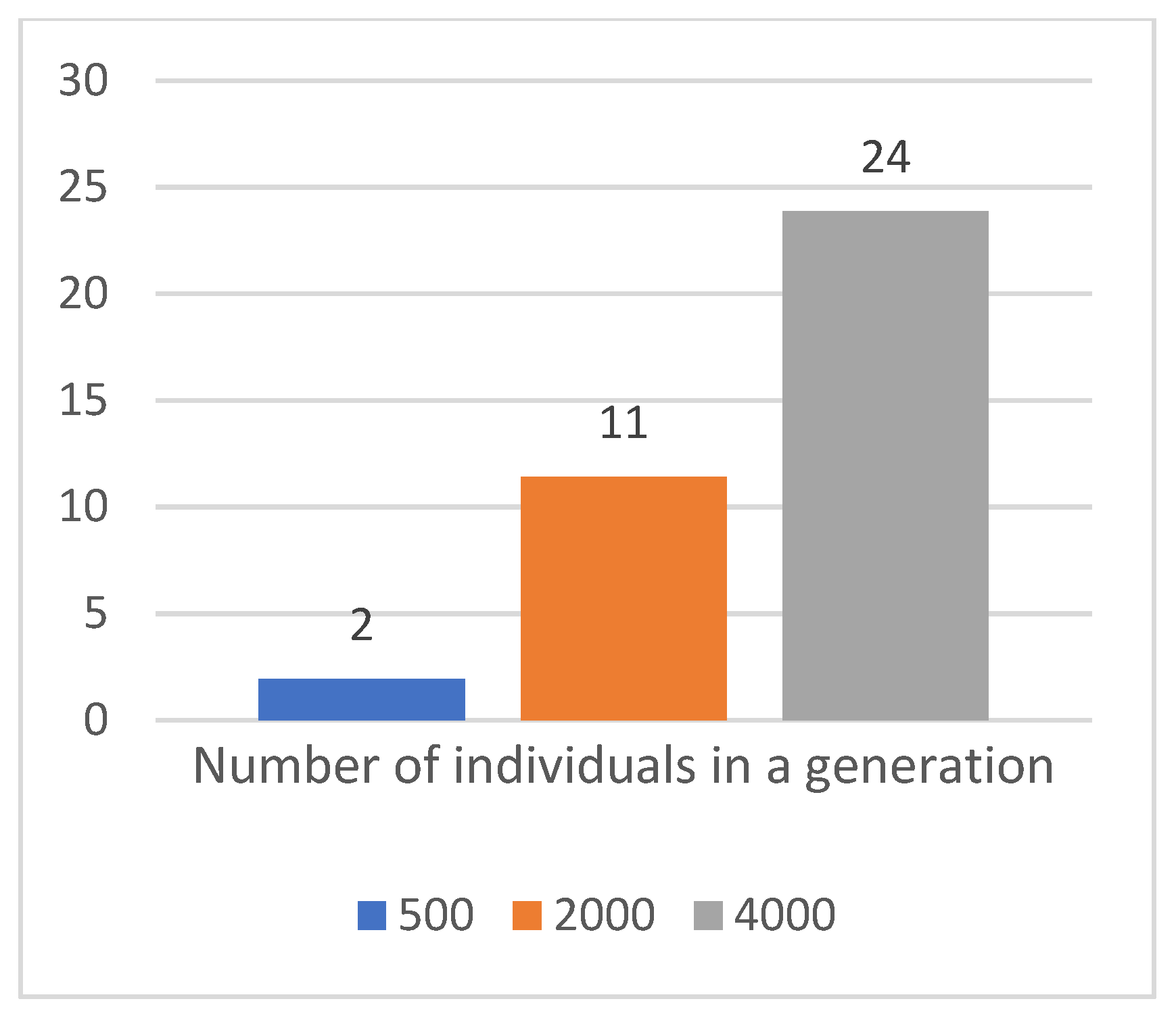
A larger number of individuals in a generation results in an improvement in both the average and median scores, as well as an increase in the scores achieved by most of the best individuals in a given evolution; indicators in the 25th and 75th percentile. However, a tribute to this improvement is the increase in the computation time required, in direct proportion to the number of individuals in the generation, see Figure 8 and Figure 9.
Next, we compared the effect of the number of individuals in a generation across topologies with different numbers of neurons in the hidden layer. For a topology with one hidden layer and different numbers of neurons, the results for a 10% mutation are set as shown in Table 6.
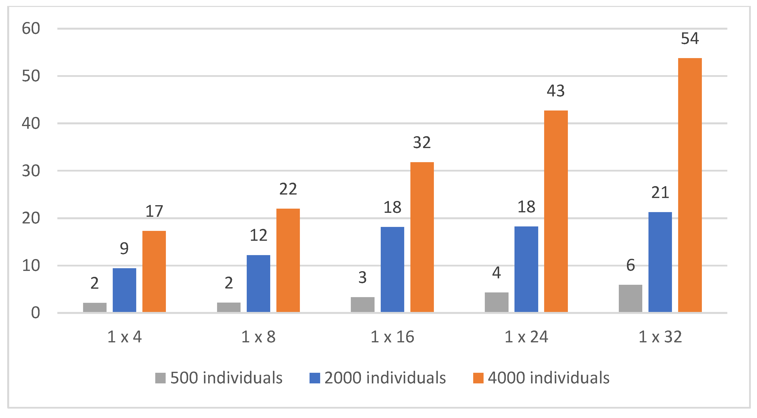
As the number of individuals in a generation increases, the results of single-individual evolutions improve, see Figure 10. On average, the best individuals perform better than in evolutions with lower numbers of individuals. However, for populations where generations have 4000 individuals, we did not see a significant improvement in terms of the top individual, i.e., the best score achieved. The best score was achieved with the 1 × 32 topology with 4000 individuals, but only with a 3% better score than the second-best one. Comparing the time required to train the NN using the GA as a function of the number of individuals in the population, we see a direct proportionality and an increase in time for populations with a higher number of individuals, see Figure 11 and Figure 12. Thus, improvements in the order of percentages are redeemed by double and multiple computational complexities.
4.2.2. Influence of the Mutation Coefficient
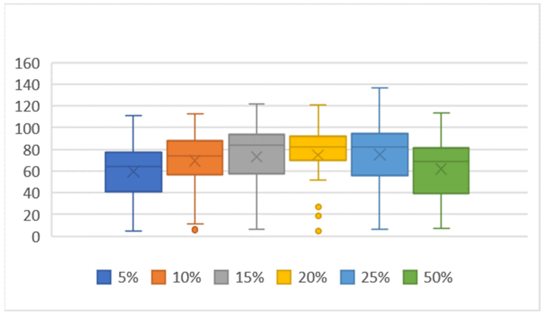
Another GA factor that can influence the results is the percentage of mutation, which indicates the percentage of neurons that undergo a random alteration of the weighting coefficients when new individuals are produced. For a comparison of 2 × 16 and 1 × 16 reference topologies with different mutation effects, see Table 7.
At a mutation factor of 15–25%, similar scores were achieved with a difference in average and medians of less than two. The best score was achieved with a mutation factor of 25%, with the computation taking the shortest time of the three mutation settings. The worst result was achieved with the 5 and 50% mutation reference settings, with the computation with the 50% mutation setting being half as fast as with the 5% mutation setting. The results of these two settings were virtually identical. The similarity of the results with a variable mutation and topology can be seen in Figure 15 and Figure 16.
Comparing the data in Table 6, we see a similar contribution of changes at the mutation level and by increasing the number of individuals in the population. However, changing the mutation rate has a minimal effect on the computation processing time, while increasing the number of individuals leads to a fold increase in the computation time.
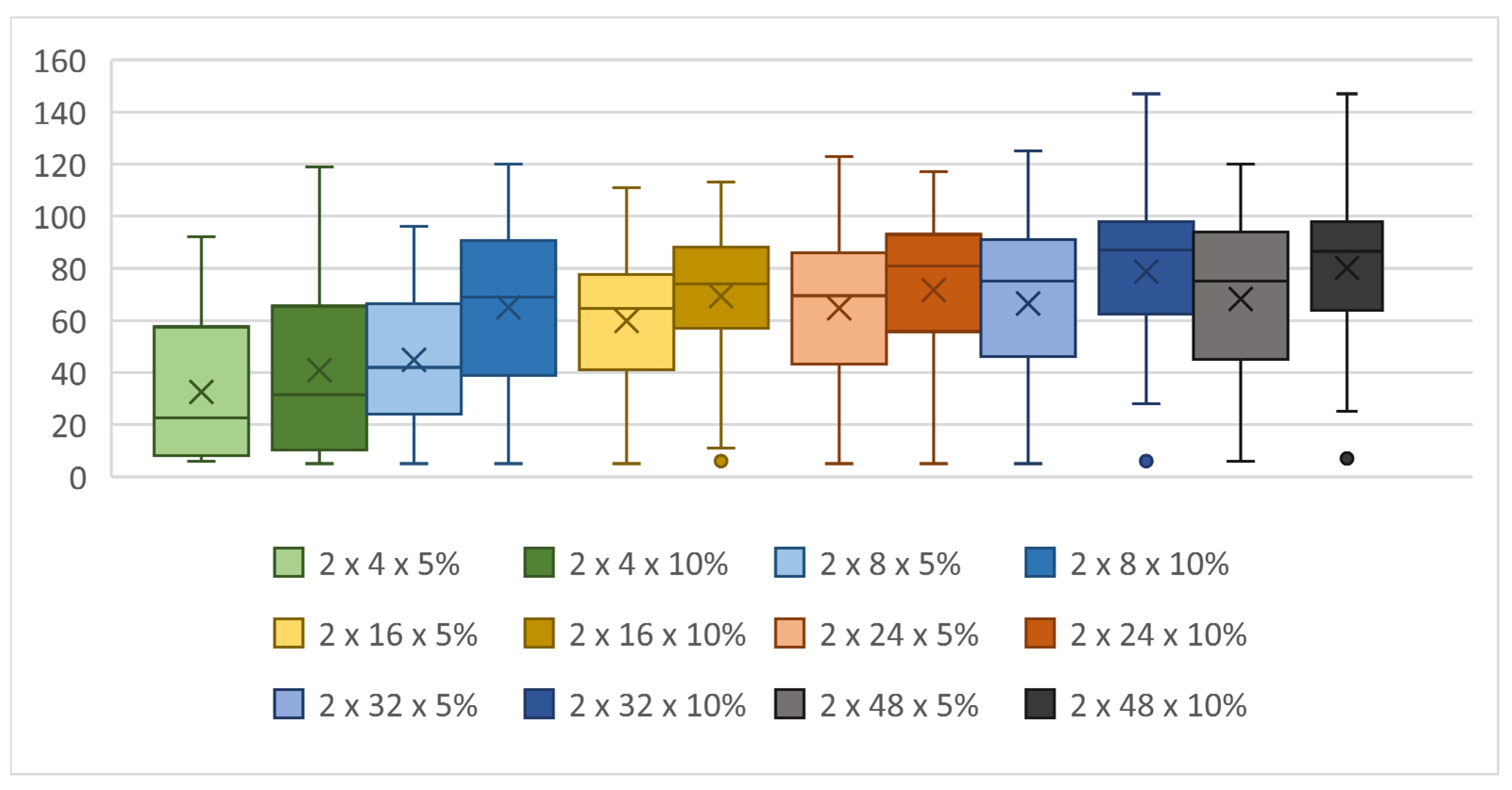
To compare the effect of a mutation as a function of the number of neurons in the hidden layers for topologies with two hidden layers, see Table 8.
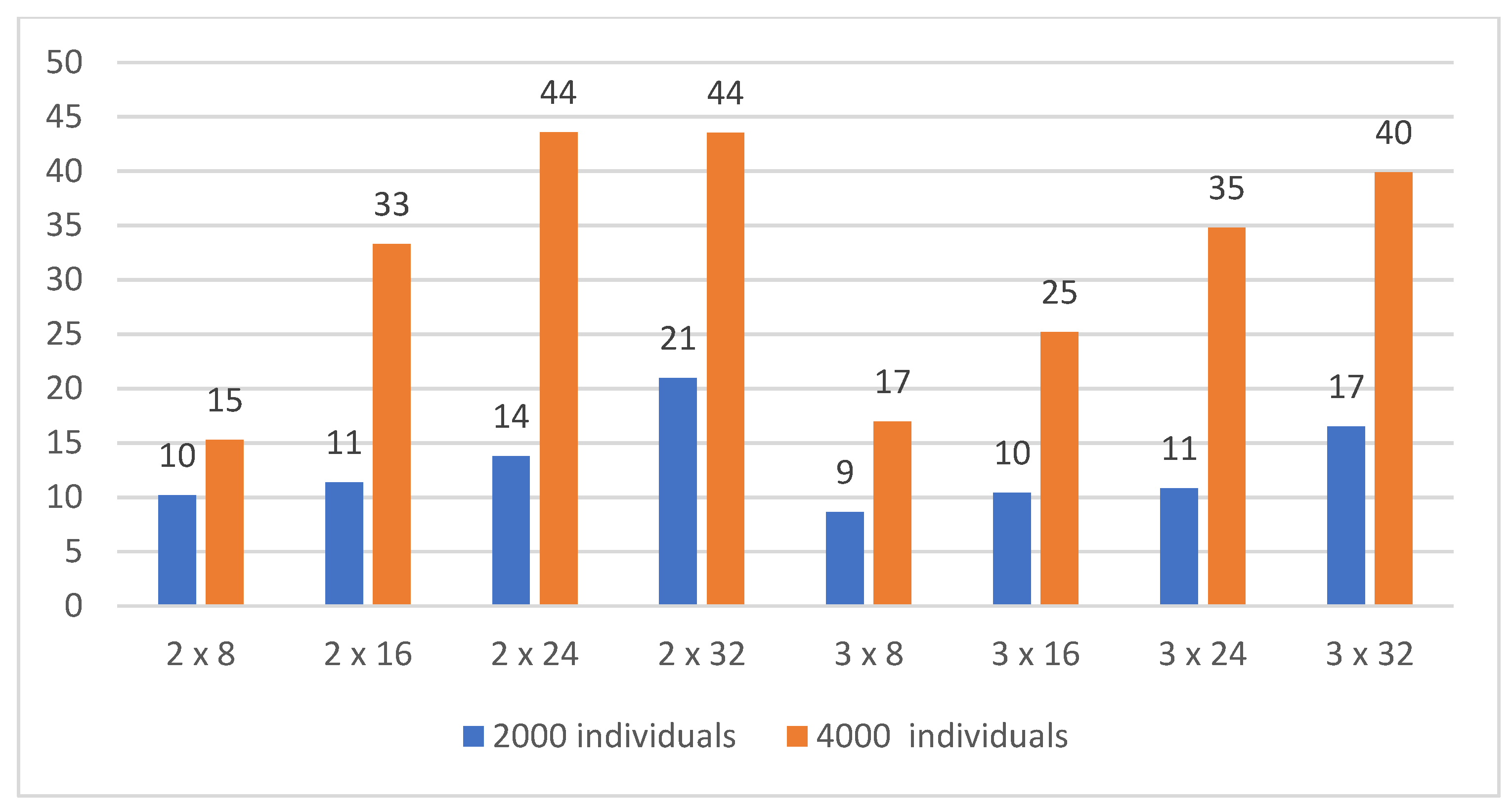
Figure 17 reveals that a 10% mutation produced significantly better results than a 5% mutation. For some topologies, the increase in both the best score and the median is more than 20%, with almost no difference in the processing time; except for the 2 × 32 topology, where the computation time was about 25% longer.
The value of the mutation rate had an effect on the achieved score, see Figure 18. With a low mutation rate of up to 5%, the population had a problem with getting stuck at the local extreme and only very slowly increased the achieved score in later generations. Whereas with high mutation rates above 25%, there was a lot of variability in the new individuals, making the results largely dependent on a chance. With a sufficient number of individuals in the population, the element of a chance may not be detrimental. The best score achieved by evolution in 50 generations of 2000 individuals was 156 with a topology of 1 × 16 and a mutation rate of 25%, see Table 7.
4.2.3. Influence of the Number of Generations
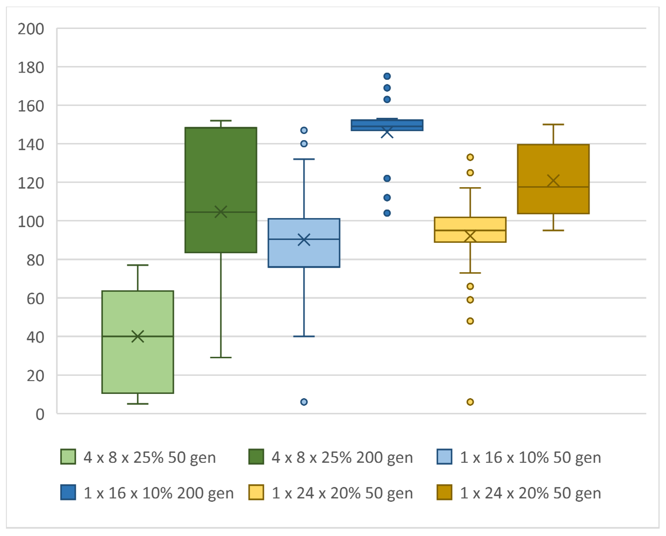
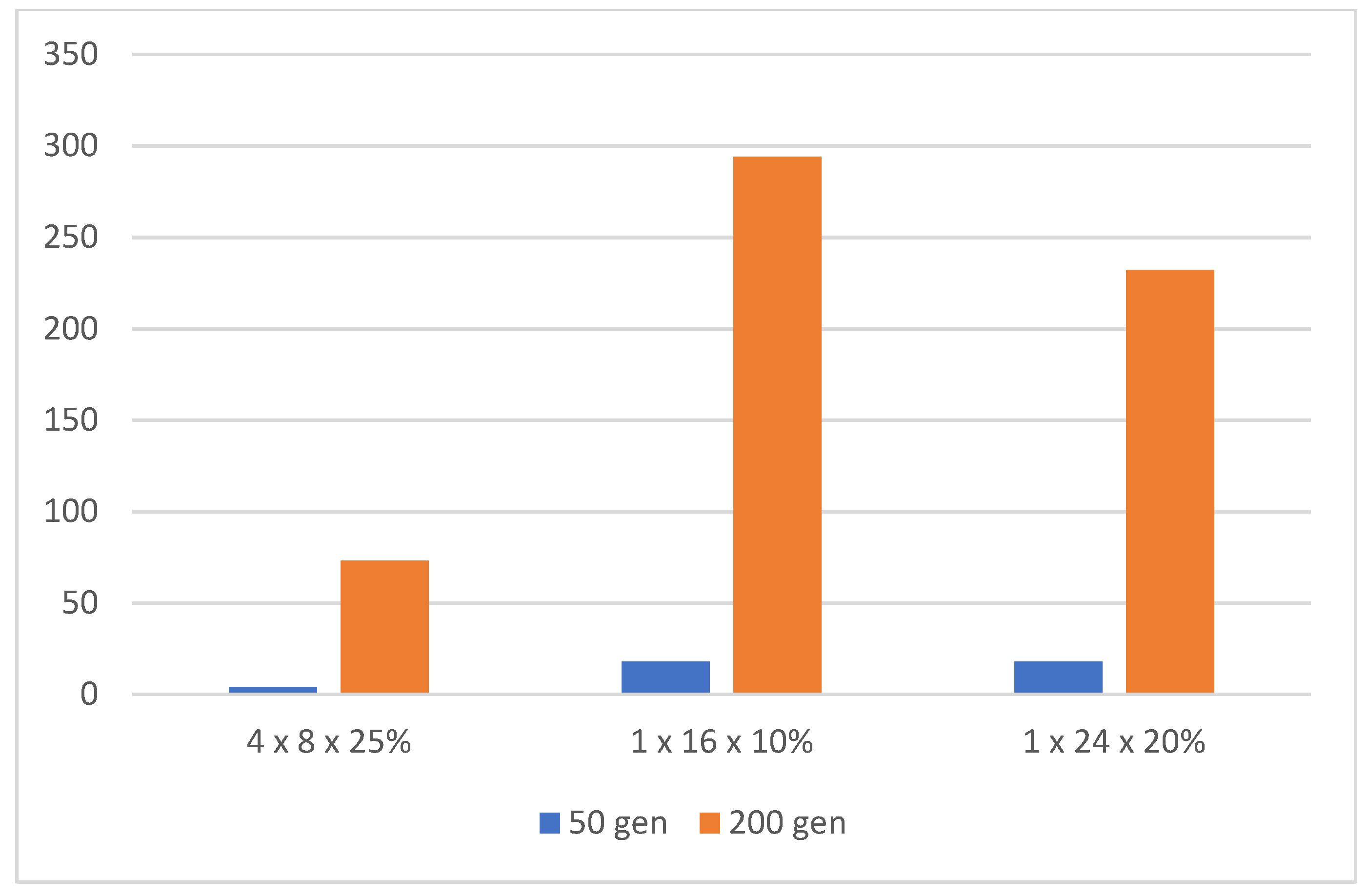
We assumed that as the number of generations increased, the score increased as well. Of course, the time required to compute the entire evolution increased with each generation. To compare the learning rate capability of the NN, we chose a single terminal attribute and that was the completion of the computation of the 50th generation in one evolution. As previously shown in the results of topologies with different numbers of hidden layers in Table 7, more complex topologies with more layers performed worse when evolutions with the same number of generations were performed. However, this did not mean that they were less suitable. As shown in Table 9 and Figure 18, the number of generations had a major impact on the scores achieved, but so did the computation runtime. Topologies with more hidden layers need more generations to train the NN.
If we increase the number of generations for which computations will be performed, more complex NN configurations will achieve results similar to simpler topologies. Simpler topologies, with one hidden layer and fewer neurons, showed a fast ability to learn and solve the problem, but gradually reached their limits and did not improve further. In addition, when verifying the configuration achieved by teaching a simple NN, typically with a small number of neurons, e.g., 1 × 4, by running it in new conditions, we find that such an NN was more error-prone. That is, it was unable to sufficiently generalize the problem. For example, if we record a 1 × 4 configuration with which the snake achieved a maximum score of 149 in one of the evolutions during learning, we find that it cannot take food that is randomly placed just next to the wall on the left. More complex topologies and topologies with more than one hidden layer are more robust to such errors. A tribute to the increasing number of generations (Table 9, Figure 19 and Figure 20) in a single evolution is a quadratically increasing computation time. If we increase the number of generations from 50 to 200, i.e., four times, the average computation time per evolution increased by about 16 times. So, we need to choose a reasonable number of generations for which the GA computation still makes sense.
4.2.4. Influence of the Number of Evolutions
In this game, it is a completely stochastic problem with different input sub-conditions each time. The goal is to find the food that appears in completely random locations each time and thus, no game proceeds in exactly the same way. Similarly, the initial generation of individuals is completely random. For each NN topology and different combinations of the number of individuals in the generations, we made 60 measurements, i.e., 60 different evolutions with a given topology. It turned out that for virtually all topologies, there was always at least one evolution that had an initial randomly generated population, such that even after 50 generations, it did not reach a score higher than 30. A score of 30 means, among others, that the resulting individual is 30 pixels long and thus does not reach the length of even one side. On the other hand, especially for simple topologies, at least one evolution managed to achieve quite an unexpectedly good score for a given topology. For example, 99 even for the 1 × 4 topology with 5% mutation and with 10% mutation even 149, and generating all 60 evolutions in both cases did not even take 9 h. It turned out that the way to achieve a satisfactory solution may be to compute for a smaller number of generations, but performed on a larger number of evolutions. In other words, we rely more on a chance to generate the initial NN configuration.
4.2.5. Best Achieved Results
It cannot be said unequivocally that some NN topologies or some specific GA parameters perform significantly better during NN training than others. Even the simplest 1 × 4 topology with its evolutionary configuration was able to generate an individual with a score of 149 after 50 generations, which ranked in the top-ten best results achieved. However, such a single-simple topology generalized poorly and, when tested in other conditions, showed more errors than the topology with a larger number of neurons. In general, the more hidden layers a topology had, the more generations it needed for training. On the other hand, such an NN better captured the complexity of the problem and made fewer errors in new conditions. By visually comparing the playing process of the best individuals with different topologies, we can also observe different tactics that individuals have developed. For the simple 1 × 4 topology, the individual chose a more direct path to the food, whereas in complex topologies, the individual tried to use the playing area space efficiently. This points to a better generalization of the problem, because with a score of around 160 points, the snake has a length that circles the playing area around its entire perimeter and mistakes are made when choosing a path that clearly prefers to reach the food, under different conditions than in training. A score value of 160 also proved to be a limit of capabilities for the topologies studied, and only two individuals managed to achieve a better score.
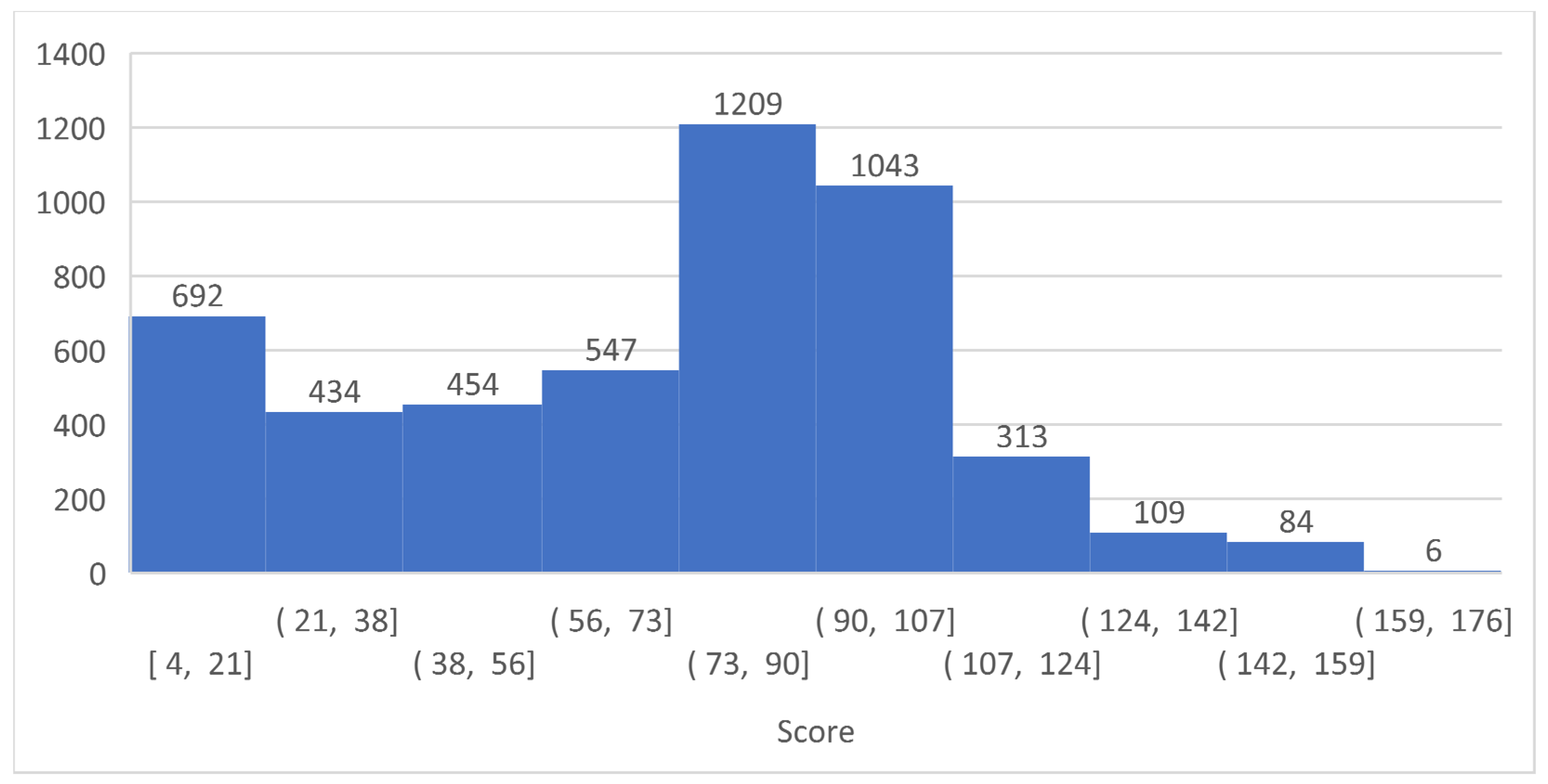
Figure 21 shows the frequency of occurrence of the achieved score in all the measurements performed.
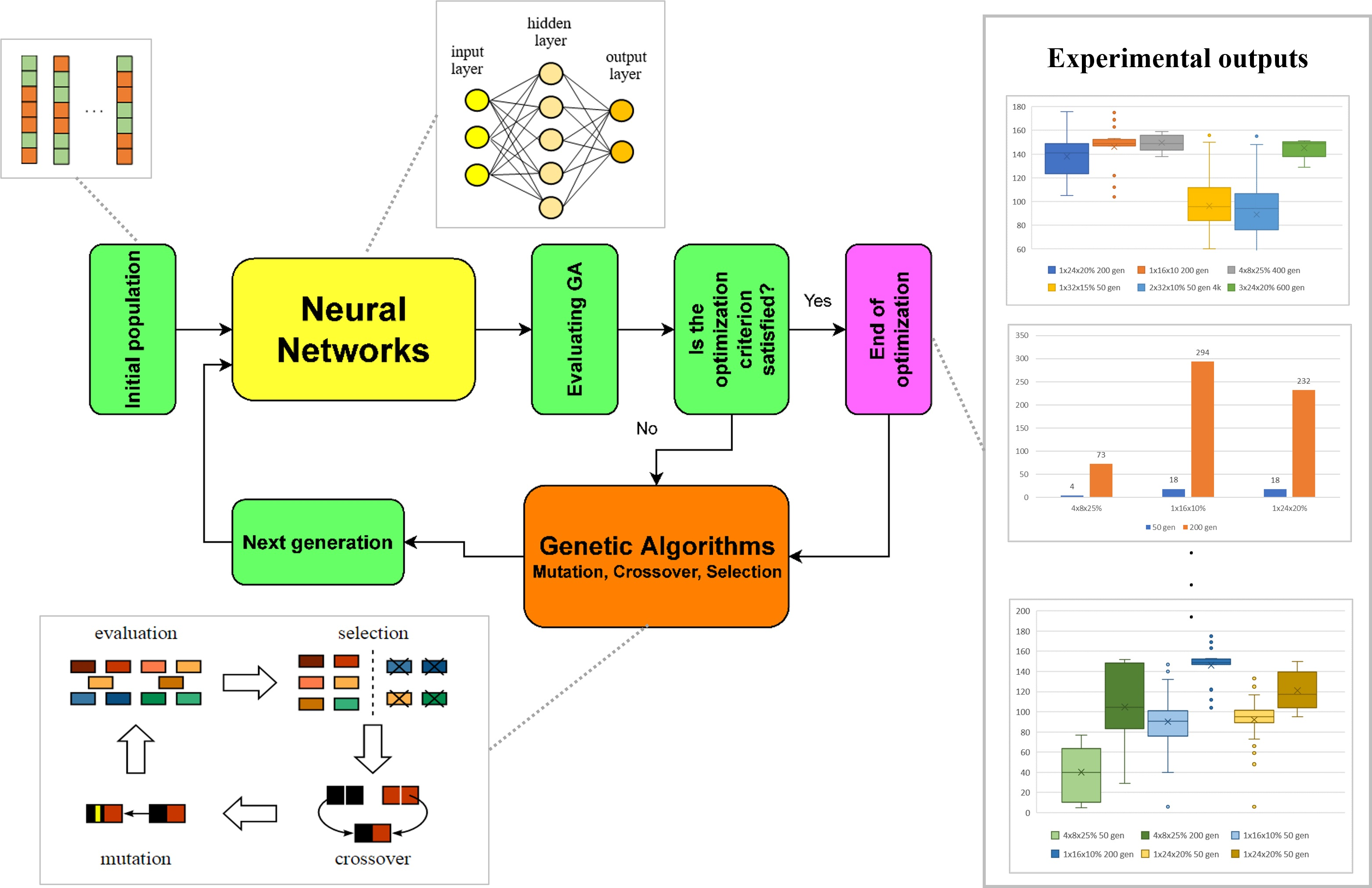
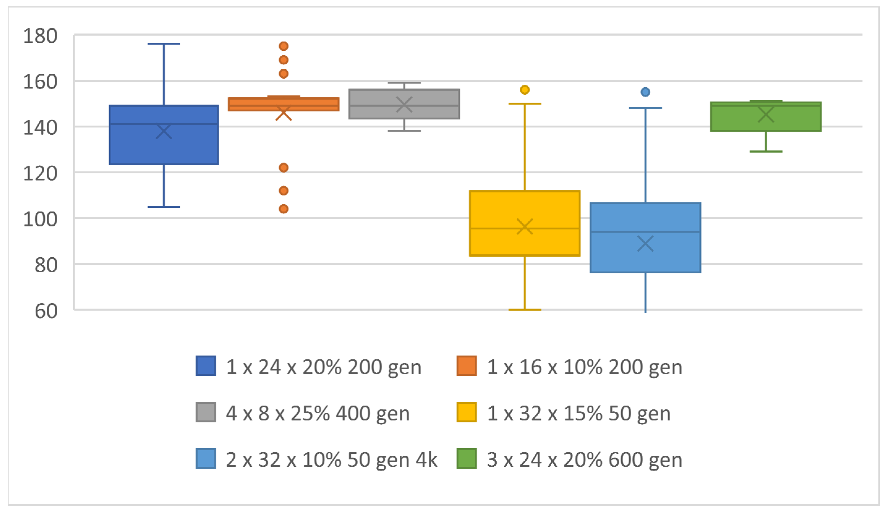
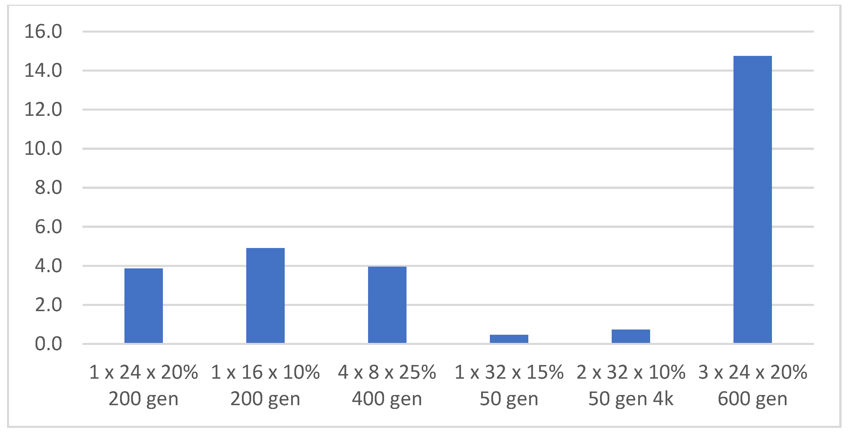
In particular, topologies with a larger number of hidden layers generated evolutions with less variance in scores between the evolution with the highest-scoring individual and the evolution that achieved the minimum score. This was true, but only if the evolution had enough generations for training. A total of 400 generations for an NN with four hidden layers, up to 600 generations for an NN with three hidden layers. The highest score of 176 was achieved with the 1 × 24 topology and 20% mutation and 200 generations per evolution. The minimum score of ten evolutions that were trained with this topology was 105. The 4 × 8 and 25% mutation topology achieved a slightly lower top score, but all five evolutions had a score of 138 or higher, which was the average of the previous topology, see Table 10. Training a single evolution was equally challenging in both cases, see Figure 21. It can be said that this configuration was not so dependent on how the weights are randomly generated in the first generation. Figure 22 shows topologies with individuals that achieved the top-six best scores and Figure 23 shows time in hours necessary to train one evolution, i.e., top score.
Table 11 provides a full comparison of the results across topologies, GA parameters versus time achieved for a particular test suite, which was stored on GitHub.
5. Evaluation of the Analysis
5.1. Ability of the Neural Network Learning
A neural network has the ability to learn and solve a problem using an evolutionary algorithm. In the case of the snake game, there is no one optimal solution. There can be virtually unlimited ways of solving and playing the game. Each one differs with a different approach and the tactics for playing it.
Unlike the methods of teaching NNs with a teacher, which in this case could be comparing single frames of game positions when played by live players with frames generated during an NN play, the evolutionary method, i.e., without a teacher, is much cheaper and faster. Creating a database of snapshots from games played would not only be tedious, but more importantly, there would have to be enough snapshots, i.e., from many games played and from a large number of players. Otherwise, the NN would assume the habits of the particular player who played the game. On the other hand, an evolutionary algorithm needs no feedback other than an evaluation of the game played, and finds out if any individual has performed better in the next game. If so, it uses the configuration to improve its own. It introduces a realm of entirely new solutions that may be very far from our idea of an ideal solution, and yet these new solutions may be sufficient or better.
For each NN topology chosen and tested, the results achieved clearly demonstrated the ability of the NNs to solve this game and score high in it. However, some, especially simpler topologies, cannot generalize well, and even if they achieved high scores when trained on a particular set of inputs, they exhibited errors while playing on another set of inputs and did not solve such a problem satisfactorily.
It was shown that as the number of neurons in the NN increased, the network better affected the breadth of the problem and such a network was able to achieve such results repeatedly with different inputs. In other words, it better generalized the problem. The disadvantage of more complex topologies with more hidden layers was the slower learning of such a network. The network needed more generations to be trained and hence a longer time. The chance element also played a much smaller role in these networks during the generation of the configuration of the first-generation individuals. In both the three- and four-hidden layer networks, individual evolutions with high generation counts achieved results with little variance, and none of the evolutions were stuck at an early local extreme, and all were able to achieve scores over 100.
5.2. Influence of the Changes in the Evolutionary Algorithm
Changes in the evolutionary algorithm parameters, such as the number of individuals in a generation, number of generations for which the whole population was generated, or the mutation coefficient, had a major impact on the score achieved and the speed of the whole learning process.
More complex NNs with a larger number of hidden layers need more generations and, thus, a much longer time to be trained. It has been shown that the time complexity increases quadratically with an increasing number of generations needed to train the NN.
A larger number of individuals in a generation leads to a more diverse population and thus to an improved score, at the cost of a linear increase in the time required to compute each generation.
On the other hand, the mutation rate had little effect on the computation time, but had a significant effect on overcoming local extremes that the population was unable to overcome in a given number of generations and, thus, evolved more slowly or not at all. However, if the mutation rate was too high, the population also stopped evolving because the number of randomly changed weights was already so large that it did not carry over the desirable learned characteristics of the individual to the next generation.
6. Conclusions and Future Work
The aim of this research is to try to find the optimal topology and train it in the shortest possible time with the help of genetic algorithms. It has been shown that more complex topologies with a larger number of neurons were not able to achieve the same results as simple topologies in a short time of training. To demonstrate the ability of NS to learn, simpler topologies with fewer neurons were sufficient. The SnakeAI project is a good didactic tool to demonstrate the ability to train an NN using an evolutionary algorithm and to teach it to play the snake game in a short time. In this research, we focused on assessing the effect of changes in NN topologies and changes in parameters in the GA on NN training performance and speed. We measured a large amount of data for different topologies and different GA parameters, which were further statistically processed to find the optimal topology and train it in the shortest time. It turned out that more complex topologies with a larger number of neurons cannot achieve the same results as simple topologies when trained in a short time. Thus, simpler topologies with fewer neurons than those used in Mr. G. Viau’s original project were sufficient to demonstrate the NN’s ability to learn. In order to speed up the training of the NN for a given task, it seems more advantageous to use a larger mutation coefficient than in the original project. Increasing it from 5 to 20% improved the results of the whole population by 20%, while the computation time only increased by 10%.
Other changes that had a positive effect on improving the scores of the whole population have already had a dramatic effect on the time required for training. A larger number of individuals in a generation resulted in a linear increase in time, a larger number of generations resulted in a quadratic increase in time, but it was necessary to train topologies with a larger number of hidden layers. Practical observation of the behavior of the trained NSs in new conditions on untrained input data has shown the need for NSs with more complex topologies. NSs with one hidden layer and a small number of neurons committed errors more frequently in the new conditions. We intend to further investigate this area in a continuation of this research, comparing the results achieved by already trained NNs on sets of new games, i.e., on entirely new data, to see which topology best generalizes the problem at hand.
The genetic algorithm also has its limits when training NNs. After reaching them, the NNs did not evolve further, or many more generations were needed to achieve only fractional improvements in the order of units of %. Therefore, it would be more appropriate to use another method to fully train the NN for further improvements in the result.
Author Contributions
Conceptualization, M.K. and E.V.; Methodology, H.H.; Software, J.C.; Validation, J.C. and M.K.; Formal analysis, H.H. and J.C.; Writing—original draft preparation, M.K.; Writing—review and editing, M.K. and E.V.; Results, M.K. and J.C. All authors have read and agreed to the published version of the manuscript.
Funding
This research was funded by the University of Ostrava specific research budget SGS.
Institutional Review Board Statement
Not applicable.
Informed Consent Statement
Not applicable.
Data Availability Statement
Data has been present in main text.
Conflicts of Interest
The authors declare no conflict of interest. The funders had no role in the design of the study; in the collection, analyses, or interpretation of data; in the writing of the manuscript, or in the decision to publish the final results.
References
- Nicholson, C. Artificial Intelligence (AI) vs. Machine Learning vs. Deep Learning. Available online: https://wiki.pathmind.com/ai-vs-machine-learning-vs-deep-learning (accessed on 1 April 2022).
- Zelinka, I. BEN–Technical Literature; Artificial Intelligence: Prague, Czech Republic, 2003; ISBN 80-7300-068-7. [Google Scholar]
- Fitzsimmons, M.; Kunze, H. Combining Hopfield neural networks, with applications to grid-based mathematics puzzles. Neural Netw. 2019, 118, 81–89. [Google Scholar] [CrossRef]
- Tian, Y.; Zhang, X.; Wang, C.; Jin, Y. An evolutionary algorithm for large-scale sparse multiobjective optimization problems. IEEE Trans. Evol. Comput. 2019, 24, 380–393. [Google Scholar] [CrossRef]
- Zolpakar, N.A.; Yasak, M.F.; Pathak, S. A review: Use of evolutionary algorithm for optimisation of machining parameters. Int. J. Adv. Manuf. Technol. 2021, 115, 31–47. [Google Scholar] [CrossRef]
- Haldurai, L.; Madhubala, T.; Rajalakshmi, R. A study on genetic algorithm and its applications. Int. J. Comput. Sci. Eng. 2016, 4, 139. [Google Scholar]
- OpenAI, Gym. Available online: https://gym.openai.com/docs/#available-environments (accessed on 25 February 2021).
- Bellemare, M.G.; Naddaf, Y.; Veness, J.; Bowling, M. The Arcade Learning Environment: An Evaluation Platform for General Agents. J. Artif. Intell. Res. 2013, 47, 253–279. [Google Scholar] [CrossRef]
- Such, F.P.; Madhavan, V.; Conti, E.; Lehman, J.; Stanley, K.O.; Clune, J. Deep neuroevolution: Genetic algorithms are a competitive alternative for training deep neural networks for reinforcement learning. arXiv 2017, arXiv:1712.06567. [Google Scholar]
- Mnih, V.; Kavukcuoglu, K.; Silver, D.; Rusu, A.A.; Veness, J.; Bellemare, M.G.; Graves, A.; Riedmiller, M.; Fidjeland, A.K.; Ostrovski, G.; et al. Human-level control through deep reinforcement learning. Nature 2015, 518, 529–533. [Google Scholar] [CrossRef]
- Comi, M. How to teach AI to play Games: Deep Reinforcement Learning. Available online: https://towardsdatascience.com/how-to-teach-an-ai-to-play-games-deep-reinforcement-learning-28f9b920440a (accessed on 27 February 2021).
- Stanislawska, K.; Krawiec, K.; Kundzewicz, Z.W. Modeling global temperature changes with genetic programming. Comput. Math. Appl. 2012, 64, 3717–3728. [Google Scholar] [CrossRef] [Green Version]
- Fisher, J.C. Optimization of Water-Level Monitoring Networks in the Eastern Snake River Plain Aquifer Using a Kriging-Based Genetic Algorithm Method; Bureau of Reclamation and U.S. Department of Energy: Reston, VA, USA, 2013.
- Fitzgerald, J.M.; Ryan, C.; Medernach, D.; Krawiec, K. An integrated approach to stage 1 breast cancer detection. In Proceedings of the 2015 Annual Conference on Genetic and Evolutionary Computation, Madrid, Spain, 11–15 July 2015; pp. 1199–1206. [Google Scholar]
- Wang, S.; Wang, Y.; Du, W.; Sun, F.; Wang, X.; Zhou, C.; Liang, Y. A multi-approaches-guided genetic algorithm with application to operon prediction. Artif. Intell. Med. 2007, 41, 151–159. [Google Scholar] [CrossRef]
- Gondro, C.; Kinghorn, B.P. A simple genetic algorithm for multiple sequence alignment. Genet. Mol. Res. 2007, 6, 964–982. [Google Scholar]
- George, A.; Rajakumar, B.R.; Binu, D. Genetic algorithm based airlines booking terminal open/close decision system. In Proceedings of the International Conference on Advances in Computing, Communications and Informatics, Chennai, India, 3–5 August 2012; pp. 174–179. [Google Scholar]
- Ellefsen, K.; Lepikson, H.; Albiez, J. Multiobjective coverage path planning: Enabling automated inspection of complex, real-world structures. Appl. Soft Comput. 2017, 61, 264–282. [Google Scholar] [CrossRef] [Green Version]
- Vidal, T.; Crainic, T.G.; Gendreau, M.; Lahrichi, N.; Rei, W. A Hybrid Genetic Algorithm for Multidepot and Periodic Vehicle Routing Problems. Oper. Res. 2012, 60, 611–624. [Google Scholar] [CrossRef]
- Chung, H.; Shin, K.-S. Genetic algorithm-optimized multi-channel convolutional neural network for stock market prediction. Neural Comput. Appl. 2019, 32, 7897–7914. [Google Scholar] [CrossRef]
- Li, Y.; Jia, M.; Han, X.; Bai, X.-S. Towards a comprehensive optimization of engine efficiency and emissions by coupling artificial neural network (ANN) with genetic algorithm (GA). Energy 2021, 225, 120331. [Google Scholar] [CrossRef]
- Hamdia, K.M.; Zhuang, X.; Rabczuk, T. An efficient optimization approach for designing machine learning models based on genetic algorithm. Neural Comput. Appl. 2020, 33, 1923–1933. [Google Scholar] [CrossRef]
- Flórez, C.A.C.; Rosário, J.M.; Amaya, D. Control structure for a car-like robot using artificial neural networks and genetic algorithms. Neural Comput. Appl. 2018, 32, 15771–15784. [Google Scholar] [CrossRef]
- Amini, F.; Hu, G. A two-layer feature selection method using Genetic Algorithm and Elastic Net. Expert Syst. Appl. 2020, 166, 114072. [Google Scholar] [CrossRef]
- Sun, Y.; Xue, B.; Zhang, M.; Yen, G.G.; Lv, J. Automatically Designing CNN Architectures Using the Genetic Algorithm for Image Classification. IEEE Trans. Cybern. 2020, 50, 3840–3854. [Google Scholar] [CrossRef] [Green Version]
- Tian, Y.; Lu, C.; Zhang, X.; Tan, K.C.; Jin, Y. Solving large-scale multiobjective optimization problems with sparse optimal solutions via unsupervised neural networks. IEEE transactions on cybernetics 2020, 51, 3115–3128. [Google Scholar] [CrossRef]
- Abiodun, O.I.; Jantan, A.; Omolara, A.E.; Dada, K.V.; Mohamed, N.A.; Arshad, H. State-of-the-art in artificial neural network applications: A survey. Heliyon 2018, 4, e00938. [Google Scholar] [CrossRef] [Green Version]
- Slowik, A.; Kwasnicka, H. Evolutionary algorithms and their applications to engineering problems. Neural Comput. Appl. 2020, 32, 12363–12379. [Google Scholar] [CrossRef] [Green Version]
- Bacalhau, E.T.; Casacio, L.; de Azevedo, A.T. New hybrid genetic algorithms to solve dynamic berth allocation problem. Expert Syst. Appl. 2021, 167, 114198. [Google Scholar] [CrossRef]
- Escamilla-García, A.; Soto-Zarazúa, G.M.; Toledano-Ayala, M.; Rivas-Araiza, E.; Gastélum-Barrios, A. Applications of Artificial Neural Networks in Greenhouse Technology and Overview for Smart Agriculture Development. Appl. Sci. 2020, 10, 3835. [Google Scholar] [CrossRef]
- Liu, L.; Moayedi, H.; Rashid, A.S.A.; Rahman, S.S.A.; Nguyen, H. Optimizing an ANN model with genetic algorithm (GA) predicting load-settlement behaviours of eco-friendly raft-pile foundation (ERP) system. Eng. Comput. 2019, 36, 421–433. [Google Scholar] [CrossRef]
- Mehmood, A.; Zameer, A.; Ling, S.H.; Rehman, A.U.; Raja, M.A.Z. Integrated computational intelligent paradigm for nonlinear electric circuit models using neural networks, genetic algorithms and sequential quadratic programming. Neural Comput. Appl. 2019, 32, 10337–10357. [Google Scholar] [CrossRef]
- Ismayilov, G.; Topcuoglu, H.R. Neural network based multi-objective evolutionary algorithm for dynamic workflow scheduling in cloud computing. Future Gener. Comput. Syst. 2020, 102, 307–322. [Google Scholar] [CrossRef]
- Padhy, N.; Singh, R.P.; Satapathy, S.C. Cost-effective and fault-resilient reusability prediction model by using adaptive genetic algorithm based neural network for web-of-service applications. Clust. Comput. 2019, 22, 14559–14581. [Google Scholar] [CrossRef]
- Viau, G. Train a Neural Network to Play Snake Using a Genetic Algorithm. Available online: https://github.com/greerviau/SnakeAI (accessed on 1 April 2022).
- Ramachandran, P.; Zoph, B.; Le, Q.V. Searching for activation functions. arXiv 2017, arXiv:1710.05941. [Google Scholar]
Figure 1.
The schematic process flow.

Figure 2.
Achieved score according to the number of layers, mutation 5%.

Figure 3.
Achieved score according to the number of neurons, two hidden layers, mutation 5%.

Figure 4.
Achieved score according to the number of neurons, one hidden layer, mutation 5%.

Figure 5.
Achieved score according to the number of neurons, two hidden layers, mutation 5%.

Figure 6.
Time required to compute evolutions according to the achieved score, 2 × 16, mutation 5%. Individuals that are able to achieve high scores in early generations are marked in red, green and yellow.
Figure 6.
Time required to compute evolutions according to the achieved score, 2 × 16, mutation 5%. Individuals that are able to achieve high scores in early generations are marked in red, green and yellow.

Figure 7.
Evolution of selected measurements in generations from Figure 6.
Figure 7.
Evolution of selected measurements in generations from Figure 6.

Figure 8.
Achieved score according to the number of individuals in the generation, topology 2 × 16, mutation 5%.
Figure 8.
Achieved score according to the number of individuals in the generation, topology 2 × 16, mutation 5%.

Figure 9.
Time in hours necessary to compute 60 evolutions based on the number of individuals in the generation, topology 2 × 16, mutation 5%.
Figure 9.
Time in hours necessary to compute 60 evolutions based on the number of individuals in the generation, topology 2 × 16, mutation 5%.

Figure 10.
Influence of the number of individuals on the achieved score in topologies with one hidden layer, mutation 10%.
Figure 10.
Influence of the number of individuals on the achieved score in topologies with one hidden layer, mutation 10%.

Figure 11.
Time in hours necessary for the computation based on the number of individuals, one hidden layer.
Figure 11.
Time in hours necessary for the computation based on the number of individuals, one hidden layer.

Figure 12.
Time in hours necessary for the computation based on the number of individuals, two and three hidden layers.
Figure 12.
Time in hours necessary for the computation based on the number of individuals, two and three hidden layers.

Figure 13.
Influence of the number of individuals on the achieved score in a topology with two hidden layers, mutation 10%.
Figure 13.
Influence of the number of individuals on the achieved score in a topology with two hidden layers, mutation 10%.

Figure 14.
Influence of the number of individuals on the achieved score in a topology with three hidden layers, mutation 10%.
Figure 14.
Influence of the number of individuals on the achieved score in a topology with three hidden layers, mutation 10%.

Figure 15.
Influence of the 2 × 16 topology.

Figure 16.
Influence of mutation on the achieved results, 1 × 16 topology.

Figure 17.
Achieved score based on a mutation in topologies with two hidden layers.

Figure 18.
Computation time of topologies with two hidden layers based on the mutation level.

Figure 19.
Influence of the number of generations in the evolution of the final score.

Figure 20.
Time in minutes necessary to train an NN based on the number of generations in the evolution.
Figure 20.
Time in minutes necessary to train an NN based on the number of generations in the evolution.

Figure 21.
Frequency of the achieved results of evolutions of all topologies.

Figure 22.
Topologies with individuals that achieved the top-six best scores.

Figure 23.
Time in hours necessary to train one evolution, top score.


Table 1.
Achieved score according to the number of layers, each of 16 neurons, mutation 5%.
| Topology: | 1 × 16 | 2 × 16 | 3 × 16 | 4 × 16 |
|---|---|---|---|---|
| Max score: | 142 | 111 | 123 | 98 |
| Min score: | 5 | 5 | 6 | 6 |
| Average: | 72 | 60 | 49 | 41 |
| Median: | 75.5 | 64.5 | 52 | 27 |
| 25th percentile: | 51 | 41 | 23 | 11 |
| 75th percentile: | 96 | 77 | 73 | 74 |
| Total processing time [h] | 17 | 11 | 11 | 4 |
Table 2.
Achieved score according to the number of neurons, two hidden layers, mutation 5%.
| Topology: | 1 × 4 | 1 × 8 | 1 × 16 | 1 × 24 | 1 × 32 | 1 × 48 | 2 × 4 | 2 × 8 | 2 × 16 | 2 × 24 | 2 × 32 | 2 × 48 | 3 × 4 | 3 × 8 | 3 × 16 | 3 × 24 | 3 × 32 |
|---|---|---|---|---|---|---|---|---|---|---|---|---|---|---|---|---|---|
| Max score: | 99 | 117 | 142 | 130 | 128 | 140 | 92 | 96 | 111 | 123 | 125 | 120 | 92 | 114 | 123 | 113 | 109 |
| Min score: | 6 | 7 | 5 | 6 | 6 | 6 | 6 | 5 | 5 | 5 | 5 | 6 | 5 | 5 | 6 | 5 | 6 |
| Average: | 54 | 60 | 72 | 82 | 76 | 87 | 33 | 45 | 60 | 65 | 67 | 68 | 24 | 41 | 49 | 52 | 57 |
| Median | 53 | 63 | 75.5 | 81 | 80 | 91.5 | 22.5 | 42 | 64.5 | 69.5 | 75 | 75 | 13.5 | 31 | 52 | 46 | 65 |
| 25th percentile | 33 | 35 | 51 | 71 | 59 | 77 | 8 | 24 | 41 | 46 | 46 | 47 | 7 | 16 | 23 | 27 | 33 |
| 75th percentile | 75 | 82 | 96 | 97 | 98 | 101 | 57 | 66 | 77 | 86 | 91 | 94 | 32 | 65 | 73 | 76 | 82 |
| Time [h] | 9 | 13 | 17 | 16 | 25 | 30 | 6 | 8 | 11 | 14 | 16 | 29 | 4 | 8 | 11 | 12 | 14 |
Table 3.
Kruskal–Wallis Test for data distribution normality.
| Factor | Statistic | df | p |
|---|---|---|---|
| Topology | 14.621 | 2 | <0.001 |
Table 4.
Dunn Post Hoc comparison test–Topologies.
| Comparison | z | Wi | Wj | p | pbonf | pholm |
|---|---|---|---|---|---|---|
| 1 × 16–2 × 16 | 2.064 | 109.150 | 89.525 | 0.020 | 0.059 | 0.039 |
| 1 × 16–3 × 16 | 3.820 | 109.150 | 72.825 | <0.001 | <0.001 | <0.001 |
| 2 × 16–3 × 16 | 1.756 | 89.525 | 72.825 | 0.040 | 0.119 | 0.040 |
Table 5.
Achieved score according to the number of individuals in the generation, topology 2 × 16, mutation 5%.
Table 5.
Achieved score according to the number of individuals in the generation, topology 2 × 16, mutation 5%.
| Topology: | 2 × 16 | 2 × 16 | 2 × 16 |
|---|---|---|---|
| Individuals in a generation | 500 | 2000 | 4000 |
| Max score: | 75 | 111 | 149 |
| Min score: | 4 | 5 | 8 |
| Average: | 28 | 60 | 76 |
| Median: | 24.5 | 64.5 | 78 |
| 25th percentile: | 7 | 41 | 64 |
| 75th percentile: | 42 | 77 | 94 |
| Total processing time [h] | 2 | 11 | 24 |
Table 6.
Influence of the number of individuals on the achieved score in topologies with one hidden layer, mutation 10%.
Table 6.
Influence of the number of individuals on the achieved score in topologies with one hidden layer, mutation 10%.
| Topology: | 1 × 4 | 1 × 4 | 1 × 4 | 1 × 16 | 1 × 16 | 1 × 16 | 1 × 32 | 1 × 32 | 1 × 32 |
|---|---|---|---|---|---|---|---|---|---|
| Number of individuals: | 500 | 2000 | 4000 | 500 | 2000 | 4000 | 500 | 2000 | 4000 |
| Max score: | 90 | 149 | 136 | 106 | 147 | 147 | 125 | 147 | 152 |
| Min score: | 5 | 5 | 8 | 5 | 6 | 25 | 5 | 5 | 37 |
| Average: | 34 | 58 | 80 | 49 | 90 | 96 | 49 | 91 | 104 |
| Median: | 27 | 53.5 | 85 | 48 | 90.5 | 97 | 51 | 93 | 102.5 |
| 25th percentile: | 8 | 31 | 70 | 20 | 76 | 83 | 17 | 79 | 88 |
| 75th percentile: | 55 | 80 | 96 | 75 | 101 | 107 | 79 | 107 | 122 |
| Total processing time [h] | 2 | 9 | 17 | 3 | 18 | 32 | 6 | 21 | 54 |
Table 7.
Influence of mutation on the achieved results, topologies 1 × 16 and 2 × 16.
| Topology: | 1 × 16 | 1 × 16 | 1 × 16 | 1 × 16 | 1 × 16 | 2 × 16 | 2 × 16 | 2 × 16 | 2 × 16 | 2 × 16 | 2 × 16 |
|---|---|---|---|---|---|---|---|---|---|---|---|
| Mutation: | 5% | 10% | 15% | 20% | 25% | 5% | 10% | 15% | 20% | 25% | 50% |
| Max score: | 142 | 147 | 150 | 150 | 156 | 111 | 113 | 122 | 121 | 137 | 114 |
| Min score: | 5 | 6 | 6 | 6 | 6 | 5 | 6 | 6 | 5 | 6 | 7 |
| Average: | 72 | 90 | 88 | 93 | 91 | 60 | 69 | 73 | 75 | 75 | 62 |
| Median: | 75.5 | 90.5 | 89 | 96 | 94 | 64.5 | 74 | 83.5 | 82.5 | 82.5 | 69 |
| 25th percentile: | 51 | 76 | 76 | 89 | 77 | 41 | 57 | 58 | 70 | 62 | 41 |
| 75th percentile: | 96 | 101 | 98 | 105 | 105 | 77 | 87 | 94 | 91 | 94 | 81 |
| Total processing time [h] | 17 | 18 | 16 | 19 | 17 | 11 | 11 | 13 | 13 | 12 | 7 |
Table 8.
Achieved score based on a mutation in topologies with two hidden layers.
| Topology: | 2 × 4 | 2 × 4 | 2 × 8 | 2 × 8 | 2 × 16 | 2 × 16 |
|---|---|---|---|---|---|---|
| Mutation: | 5% | 10% | 5% | 10% | 5% | 10% |
| Max score: | 92 | 119 | 96 | 120 | 111 | 113 |
| Min score: | 6 | 5 | 5 | 5 | 5 | 6 |
| Average: | 33 | 41 | 45 | 65 | 60 | 69 |
| Median: | 22.5 | 31.5 | 42 | 69 | 64.5 | 74 |
| 25th percentile: | 8 | 13 | 24 | 40 | 41 | 57 |
| 75th percentile: | 57 | 65 | 66 | 90 | 77 | 87 |
| Total processing time [h] | 6 | 5 | 8 | 10 | 11 | 11 |
| Topology: | 2 × 24 | 2 × 24 | 2 × 32 | 2 × 32 | 2 × 48 | 2 × 48 |
| Mutation: | 5% | 10% | 5% | 10% | 5% | 10% |
| Max score: | 123 | 117 | 125 | 147 | 120 | 147 |
| Min score: | 5 | 5 | 5 | 6 | 6 | 7 |
| Average: | 65 | 72 | 67 | 79 | 68 | 80 |
| Median: | 69.5 | 81 | 75 | 87 | 75 | 86.5 |
| 25th percentile: | 46 | 57 | 46 | 66 | 47 | 66 |
| 75th percentile: | 86 | 93 | 91 | 98 | 94 | 98 |
| Total processing time [h] | 14 | 14 | 16 | 21 | 29 | 28 |
Table 9.
Influence of the number of generations on the final score.
| Topology: | 4 × 8 | 4 × 8 | 1 × 16 | 1 × 16 | 1 × 24 | 1 × 24 |
|---|---|---|---|---|---|---|
| Mutation: | 25% | 25% | 10% | 10% | 20% | 20% |
| Number of generations: | 50 | 200 | 50 | 200 | 50 | 200 |
| Number of evolutions: | 20 | 10 | 60 | 20 | 60 | 10 |
| Max score: | 77 | 152 | 147 | 175 | 133 | 150 |
| Min score: | 5 | 29 | 6 | 104 | 6 | 95 |
| Average: | 40 | 105 | 90 | 146 | 92 | 121 |
| Median: | 40 | 104.5 | 90.5 | 149 | 95 | 117.5 |
| 25th percentile: | 12 | 95 | 76 | 147 | 89 | 106 |
| 75th percentile: | 63 | 141 | 101 | 151 | 101 | 133 |
| Total processing time [h] | 1 | 12 | 18 | 98 | 18 | 39 |
Table 10.
Topologies with individuals that achieved the top-six best scores.
| Topology: | 1 × 24 × 20% | 1 × 16 × 10% | 4 × 8 × 25% | 1 × 32 × 15% | 2 × 32 × 10% | 3 × 24 × 20% |
|---|---|---|---|---|---|---|
| Number of generations: | 200 | 200 | 400 | 50 | 50 | 600 |
| Number of individuals | 2000 | 2000 | 2000 | 2000 | 4000 | 2000 |
| Number of evolutions: | 10 | 20 | 5 | 60 | 60 | 5 |
| Max score: | 176 | 175 | 159 | 156 | 155 | 151 |
| Min score: | 105 | 104 | 138 | 5 | 6 | 129 |
| Average: | 138 | 146 | 150 | 96 | 89 | 145 |
| Median: | 141 | 149 | 149 | 95.5 | 94 | 149 |
| 25th percentile: | 125 | 147 | 149 | 85 | 77 | 147 |
| 75th percentile: | 149 | 151 | 153 | 111 | 106 | 150 |
| Total processing time [h] | 39 | 98 | 20 | 27 | 44 | 74 |
| Processing time of evolution [h] | 3.9 | 4.9 | 4.0 | 0.5 | 0.7 | 14.7 |
Table 11.
Best achieved results across topologies.
| File Name | Topology | GA Parameters | Score | Time | |||
|---|---|---|---|---|---|---|---|
| H | N | Mut | Gen | Individ. | min | ||
| T1×24m20G200R6bestSnake_176.csv | 1 | 24 | 20 | 200 | 2000 | 176 | 210 |
| T1×16m10G200R12bestSnake_175.csv | 1 | 16 | 10 | 200 | 2000 | 175 | 353 |
| T4×8m25G400R1bestSnake_159.csv | 4 | 8 | 25 | 400 | 2000 | 159 | 252 |
| T1×32m15G50R47bestSnake_156.csv | 1 | 32 | 15 | 50 | 2000 | 156 | 42 |
| T1×16m25G50R28bestSnake_156.csv | 1 | 16 | 25 | 50 | 2000 | 156 | 28 |
| T2×32m10G50R35bestSnake4000_155.csv | 2 | 32 | 10 | 50 | 4000 | 155 | 96 |
| T4×8m25G200R1bestSnake_152.csv | 4 | 8 | 25 | 200 | 2000 | 152 | 109 |
| T1×32m10G50R14bestSnake4000_152.csv | 1 | 32 | 10 | 50 | 4000 | 152 | 73 |
| T3×24m20G600R5bestSnake_151.csv | 3 | 24 | 20 | 600 | 2000 | 151 | 914 |
| T1×4m10G50R16bestSnake_149.csv | 1 | 4 | 10 | 50 | 2000 | 149 | 28 |
| T2×16m15G50R43bestSnake4000_149.csv | 2 | 16 | 15 | 50 | 4000 | 149 | 41 |
| T2×24m10G50R9bestSnake4000_149.csv | 2 | 24 | 10 | 50 | 4000 | 149 | 60 |
| T3×48m10G50R5bestSnake4000_147.csv | 3 | 48 | 10 | 50 | 4000 | 147 | 107 |
| T3×16m10G50R46bestSnake4000_147.csv | 3 | 16 | 10 | 50 | 4000 | 147 | 58 |
Publisher’s Note: MDPI stays neutral with regard to jurisdictional claims in published maps and institutional affiliations. |
© 2022 by the authors. Licensee MDPI, Basel, Switzerland. This article is an open access article distributed under the terms and conditions of the Creative Commons Attribution (CC BY) license (https://creativecommons.org/licenses/by/4.0/).
Share and Cite
MDPI and ACS Style
Kotyrba, M.; Volna, E.; Habiballa, H.; Czyz, J. The Influence of Genetic Algorithms on Learning Possibilities of Artificial Neural Networks. Computers 2022, 11, 70. https://0-doi-org.brum.beds.ac.uk/10.3390/computers11050070
AMA Style
Kotyrba M, Volna E, Habiballa H, Czyz J. The Influence of Genetic Algorithms on Learning Possibilities of Artificial Neural Networks. Computers. 2022; 11(5):70. https://0-doi-org.brum.beds.ac.uk/10.3390/computers11050070
Chicago/Turabian StyleKotyrba, Martin, Eva Volna, Hashim Habiballa, and Josef Czyz. 2022. "The Influence of Genetic Algorithms on Learning Possibilities of Artificial Neural Networks" Computers 11, no. 5: 70. https://0-doi-org.brum.beds.ac.uk/10.3390/computers11050070
Note that from the first issue of 2016, this journal uses article numbers instead of page numbers. See further details here.