
Traffic Request Generation through a Variational Auto Encoder Approach


ENEA, Robotics and Artificial Intelligence Laboratory, Casaccia Research Centre, 00123 Rome, Italy
*
Author to whom correspondence should be addressed.
Computers 2022, 11(5), 71; https://0-doi-org.brum.beds.ac.uk/10.3390/computers11050071
Submission received: 4 April 2022
/
Revised: 22 April 2022
/
Accepted: 27 April 2022
/
Published: 29 April 2022
(This article belongs to the Special Issue Selected Papers from ICCSA 2021)
Abstract
:Traffic and transportation forecasting is a key issue in urban planning aimed to provide a greener and more sustainable environment to residents. Their privacy is a second key issue that requires synthetic travel data. A possible solution is offered by generative models. Here, a variational autoencoder architecture has been trained on a floating car dataset in order to grasp the statistical features of the traffic demand in the city of Rome. The architecture is based on multilayer dense neural networks for encoding and decoding parts. A brief analysis of parameter influence is conducted. The generated trajectories are compared with those in the dataset. The resulting reconstructed synthetic data are employed to compute the traffic fluxes and geographic distribution of parked cars. Further work directions are provided.
1. Introduction
Transportation forecasting is the attempt to estimate the number of vehicles or people that will use a specific transportation facility in the future. This can be considered a relevant subject of urban computing: the process of tackling the major issues that cities face using heterogeneous data collected by a diversity of sources in urban areas [1].
With the present fast rate of urbanization all around the world, the city populations are increasing exponentially together with the number of vehicles, causing countless traffic problems. This in turn provokes direct economic losses as well as indirect ones such as the health problems deriving from air pollutants.
Thus, transportation forecasting becomes a key issue in urban planning, possibly helping in the resolution of the conflict between traffic volume requests on one side and traffic infrastructure supply on the other [2].
Among the different approaches to the problem of traffic modeling, activity-based models are a group that try to predict for individuals where and when specific activities (e.g., work, leisure, and shopping) are carried out [3]. The idea behind activity-based models is that travel demand is derived from activities that people need or wish to perform; travel is then seen as a by-product of an agenda, as a component of an activity scheduling decision.
Traffic modeling can be primarily considered as a statistical approach and is heavily grounded on the collection of large quantities of data. People can be of extreme help in this, since they generate data during their daily activities and movements, for instance by carrying and using a mobile phone. Data can be collected through many different means, e.g., using CDRs (call detail records) from cellular phones, social network posting, vehicle or smartphone navigation data, and floating car data (FCD).
There is substantial agreement in the literature that human mobility can be seen as a highly structured domain composed of mostly regular daily/weekly schedules, showing high predictability across diverse populations [4]. Further analysis also suggests that human mobility shows temporal and spatial regularities [5,6].
It is evident that an accurate modeling of urban traffic flow may help in reducing traffic congestions, resulting in a healthier environment. On the other hand, how is it possible to reach those goals and protect privacy at the same time? Trajectory data are commercially very valuable (e.g., geographically targeted advertisements) and contain rich information about people’s travel patterns and their interactions with the urban built environment. However, users’ privacy is easily violated: it is possible to infer home/work location and socioeconomic status of a user even from social media check-in data only [7].
Traveling information should be gathered anonymously in order to protect the people’s right to privacy. In addition to this central fact, there are further concerns linked to the actual availability of data. Often, these datasets represent a limited sample of the entire population, and the data are often biased or have a low sampling rate, hence being of only partial usefulness for analyses. Furthermore, the data may belong to private enterprises (e.g., cellular phone records), adding further difficulties in availability or usability.
The main contribution of this paper is in presenting a machine learning approach to model the traffic demand in an urban area and to produce synthetic mobility data in place of real ones. A variational autoencoder (VAE) [8] based on a dense neural network architecture is used. Such a generative model can retain the statistical properties of the real data, but privacy risks can be alleviated, and data abundance issues mitigated, through the production of artificial trajectories.
The data used for the training of the model is an FCD dataset of the trajectories of a large group of private cars in the town of Rome. The data have been processed to switch towards a representation in terms of the stops separating various car trips, creating what can be called stop trajectories. To a certain extent, the use of this representation can be considered an activity-based approach, since people drive their cars from one place to another to pursue scheduled activities. An application of the presented processing pipeline is provided, where the traffic fluxes and geographic distribution of parked cars are computed.
In the second section of the paper, the related work is briefly presented. In the third section, variational autoencoders are concisely presented, the employed dataset is described with some associated statistical analyses, and the tuning of some of the model parameters used during training is shown. In the fourth section, results are provided both in terms of generated stop trajectories and in reconstructed trajectories. The model is used to compute the traffic fluxes and geographic distribution of parked cars as an example. In Section 5, a discussion and conclusions are provided.
2. Related Work
As described above, traffic modeling, in addition to the modeling itself, should also tackle the related privacy issues and the question of data abundance. In the literature, there are several different approaches to these questions. A possible solution to overcome these concerns is to employ generative models, as it has recently been proposed in several fields of application [8]. The basic idea is represented by a generative model that is trained over the dataset of interest and then used to produce synthetic records.
A generative model can be briefly described as follows. Let us assume a dataset of observations with a given unknown statistical distribution Pdata. A generative model Pmod is designed to mimic Pdata; thus, in order to generate new observations distributed as Pdata, it would be possible to sample Pmod instead [8]. The model is trained with the observation data, and it can learn a compact feature space, the so-called latent space, the sampling of which outputs new observation data with the same statistical properties of the original ones. This clearly overcomes both the problem of user privacy, since it is essentially synthetic data, and the risk of datasets that are too small, since it is possible to generate as many data as needed.
In [9], travelers’ activity patterns are inferred from CDRs using IO-HMM with a contextual condition to the transition probability, since the information on activities is part of the dataset. In [10], this approach is pipelined to a long short term memory (LSTM) architecture to learn the traveler’s sequences, while in [11], a statistical approach is used through a dynamic Bayesian network to estimate daily mobility patterns, refining it by rejection sampling. In [12], a two-step model is devised: the first generates a mobility diary through Markov models from the real mobility data, analyzing the temporal patterns of human mobility. The second translates the diary into trajectories, i.e., a spatial analysis, on the concept of preferential return and preferential exploration.
However, most of the more recently published literature makes use of a generative model, either generative adversarial networks (GANs) [13] or autoencoders and variational autoencoders (VAEs) [8], which are able to add a stochastic component that helps in producing both good data modeling and generation.
In [14], the architecture employs a sequence-to-sequence LSTM network as arranged in a VAE to learn trajectories with high granularity. The mean distance error (MDE) between single real trajectories and reconstructed ones is used for evaluating the performance, but the overall distributions are not taken into account as an evaluation metric. In [15], a recurrent neural network is trained to learn the trajectories and is then used to produce new sequences, with a careful analysis of the produced trajectories in terms of accuracy and data privacy. The approach requires a preprocessing step to identify the home and work locations of each individual. The performances are evaluated on metrics related to the time spent per location, trip distances, and visited location per user. There is no stochastic component in the model. In [16], an adversarial network approach is used based on LSTM networks, using a trajectory encoding model, while in [17], the adversarial networks are used to train a non-parametric model that generates location trajectories on a grid, using a sparse location map, not targeted on the stops.
In the approach presented here, the used stop trajectories are a more compact data representation, which consent the use of a simpler VAE architecture based on dense neural networks. Furthermore, the stop spatial locations are directly expressed in terms of latitudes and longitudes, instead of using discretization of higher granularity, and the spatial-temporal distributions of the dataset are reconstructed, producing synthetic stop trajectories.
3. Materials and Methods
3.1. Variational Autoencoders as Generative Models
An autoencoder can be implemented with an artificial neural network that is used to learn efficient data encodings in an unsupervised manner. The autoencoder is generally composed of two subsections, an encoder and a decoder, which are linked by an internal latent space. The trick is that the latent space dimension is significantly smaller than the input one, which is the same as the output, so the model is forced to discover and efficiently internalize the essence of the data. During the training, the system learns to reproduce in output the same data given in input. Once it has been trained, it is possible to generate new output data via the sampling of the latent space. A further refinement of these models is represented by the variational autoencoders, which are able to add a stochastic component in the latent space that helps in producing better data modeling and generation [8].
In previous work [18], a VAE composed of an LSTM model has been used, since it is a recursive neural network proficient in modeling sequences [19]. Here, a dense multi-layer perceptron has been employed for the encoder and the decoder parts of the VAE. The encoder encodes a sequence of places visited by a driver during a temporal interval of a day to its stochastic latent space, and a symmetrical dense model decodes it to the output stop-trajectory sequence, which is made by matching it as much as possible to the input sequence during the training phase.
Once trained, the latent space can be normally sampled in order to produce trajectory sequences similar, in a statistical sense, to those of the training dataset. The migration from the LSTM to the dense models stems from the much simpler configuration of stop-trajectories as compared to full trajectory samples. It is common when modeling short sequences to use a multilayer perceptron or a convolutional neural network, as these are more manageable [20].
3.2. The Dataset
The available OCTO Telematics [21] dataset is an FCD collection containing one month of records from a set of about 150,000 cars in the geographical area of Rome, Italy. Each record consists of time, position, speed, the distance from preceding record point, engine status (running, turning off, or starting), and the numerical ID of the car. The records are stored as soon as either a given time interval has passed or a given distance is traveled, and the starting or switching off of the engine are recorded events. In short, the dataset is composed of geographical points along car routes. At this stage, the user privacy is represented by the anonymity of the car ID.
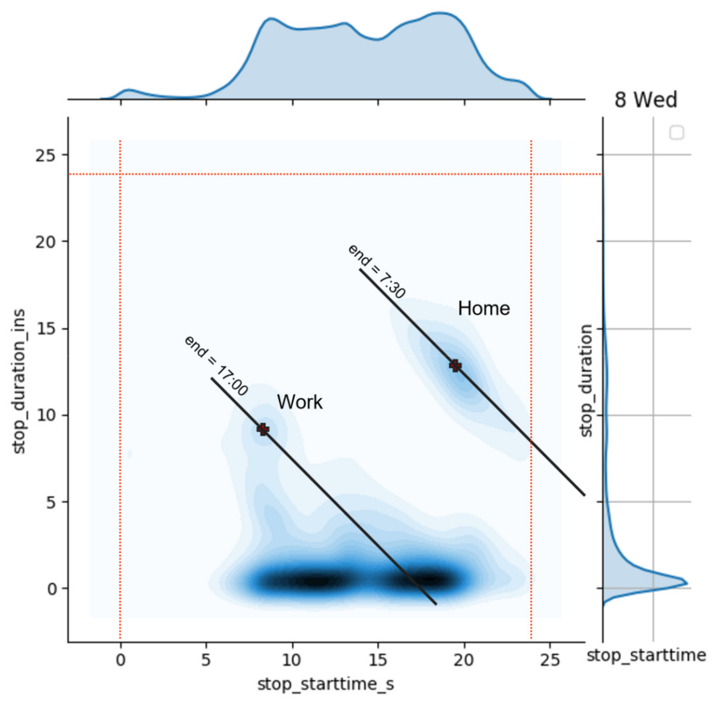
The first step was that of cleaning the dataset from unreliable data, e.g., geographical positions in the sea or sequences without starting or ending points. The processed dataset was analyzed to extract some global characteristics. As an example, Figure 1 shows an interesting analysis in terms of stops, where a stop has been defined as a turning off of the car engine for more than 5 min. The average number of stops per day on the whole dataset is 4.99 and 4.04, respectively, on weekdays and weekends/holidays.
In Figure 1, the bivariate histogram of stops in terms of the stop starting time and the stop duration is plotted.
In the figure, at least three areas can be identified: an approximately linear one on the lower part, a blob on the central left part, and a second, slightly higher blob on the right. The first group, by far the most numerous, is made up of all short-term stops, less than or equal to 1 h, more or less evenly distributed throughout the day. A series of secondary activities, such as shopping and accompanying children to school, can fall into this grouping. The blob on the right side is approximately centered on a duration of 12–13 h and a start time of around 19:30. It is considerably less numerous than the previous one, and it can be considered that of the residences, where the stops are made only once a day. A residence refers to a place where a vehicle is parked overnight for a certain number of hours: for example, the residence of a commercial vehicle may also be considered the place where it is left for the night.
To help the interpretation of Figure 1, a straight line has been drawn that passes through the center of the blob, which represents the geometric locus of all stops ending at the same time. The data in the blob are elongated in the direction of the straight line, supporting the hypothesis that the residences are being considered.
The third blob identified may be composed of stops relating to the work activities of people employed 8 h a day (full time). In fact, it is centered approximately at 8:00 with a duration of approximately 9 h, which leads to an end stop time at 17:00.
This kind of analysis may be of help to classify the activities performed at the stops, e.g., to distinguish overnight stops from work or leisure ones, and compute residences.
This type of analysis was repeated on all of the days of the dataset, indicating two macro classes of days, one for the working week (Monday–Friday), shown in Figure 1, and one for holidays and weekends, where the third blob, the one relating to offices, basically disappears.
It is interesting here to observe that Figure 1 is very similar to a figure shown in [9]. The positions and dimensions of the above three blobs are practically superimposable. This is interesting, as the data used here relates to the GPS tracks of vehicles in the city of Rome, while in [9], the CDRs of cell phones in the San Francisco Bay Area are analyzed, and activities are considered. However, if a car stop is considered as a proxy for an activity of some kind, the similarity can be explained. Another similarity is represented by the average number of activities carried out in the two cities, i.e., the average number of stops. In our dataset, there are 4.99 stops/day on weekdays and 4.04 stops/day on holidays and weekends; in [9], these values are 4.4 and 4.0.
Because of this and further statistical analyses of the dataset, a stop-based dataset composed of sequences containing a maximum of 8 stops per day was used. In the following, we refer to these sequences as stop-trajectories. Each point in a stop-trajectory is described by 6 quantities: latitude, longitude, duration, start time, day of week, and trip distance covered to reach the current stop (see Table 1). Thus, a daily trajectory is represented by 48 values; if the number of daily stops is smaller than 8, the data are padded with zeroes; if a given driver performs more than 8 stops, it is discarded (all of the trajectories of the driver are discarded to avoid data distortion). Under the above assumptions, a fraction of 50% of all available drivers is retained.
3.3. Training
The VAE dense model was trained on the subset of the dataset comprising the drivers with the considered limit on the number of stops, which means more than 900,000 different trajectories.
An analysis of the influence of the various features of the architecture on training was performed and is presented here.
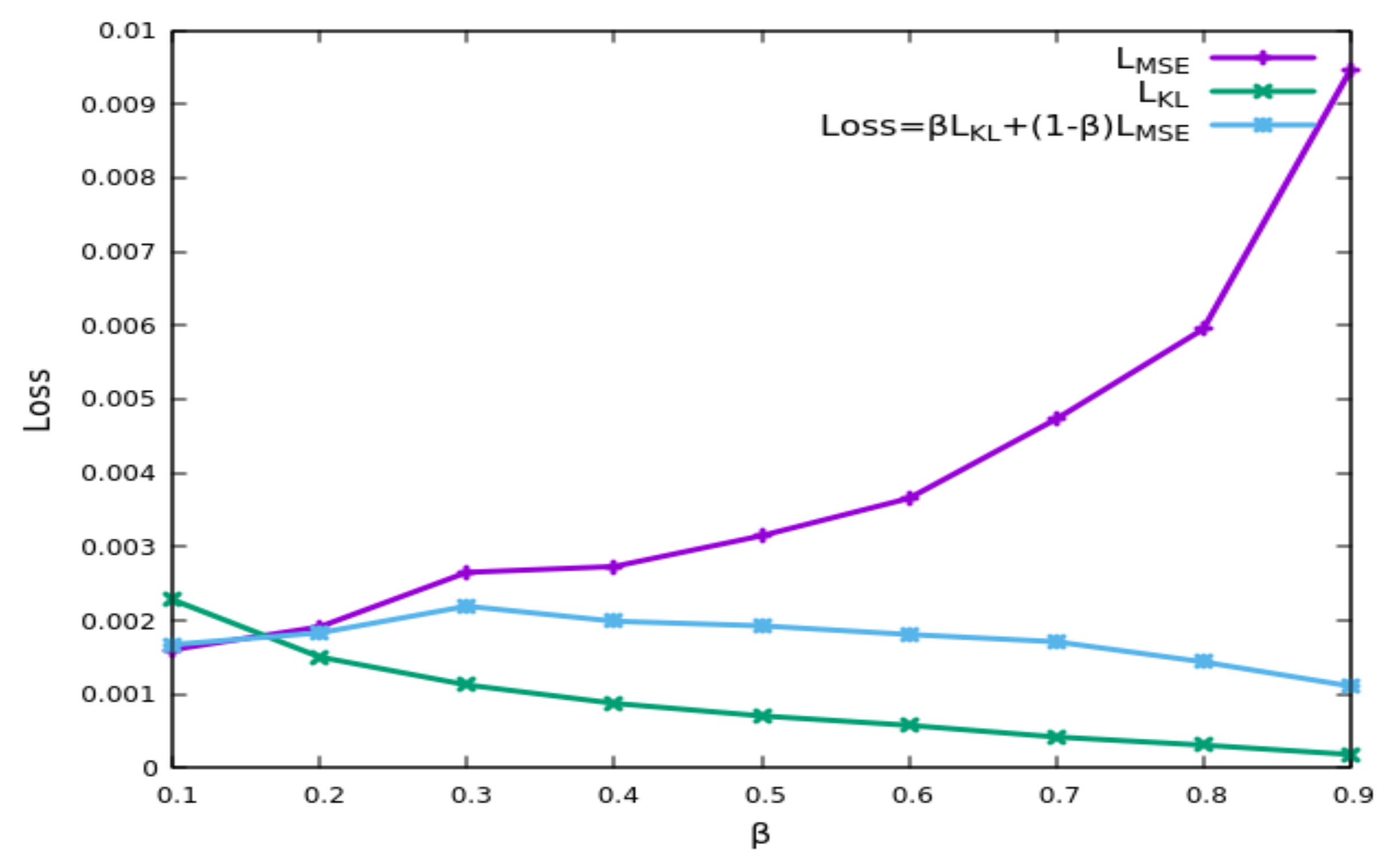
The loss function of a VAE is usually composed of two terms: a reconstruction loss describing how well the output matches the input and a regularization term helping in achieving a multivariate normal distribution in the latent space. In this work, the influence of the two terms is tuned through the following equation:
where LMSE is the reconstruction loss, typically measured by the mean squared error, and LKL is the regularization loss, typically assessed with the Kullback–Leibler divergence. Figure 2 shows the final loss behavior versus the β term. If a large value for β is chosen, the influence of the MSE decreases, and the reconstruction error increases. If a value of 0.2 for the trade-off parameter β is chosen, a low value for the MSE can be reached while maintaining a limited KL-divergence.
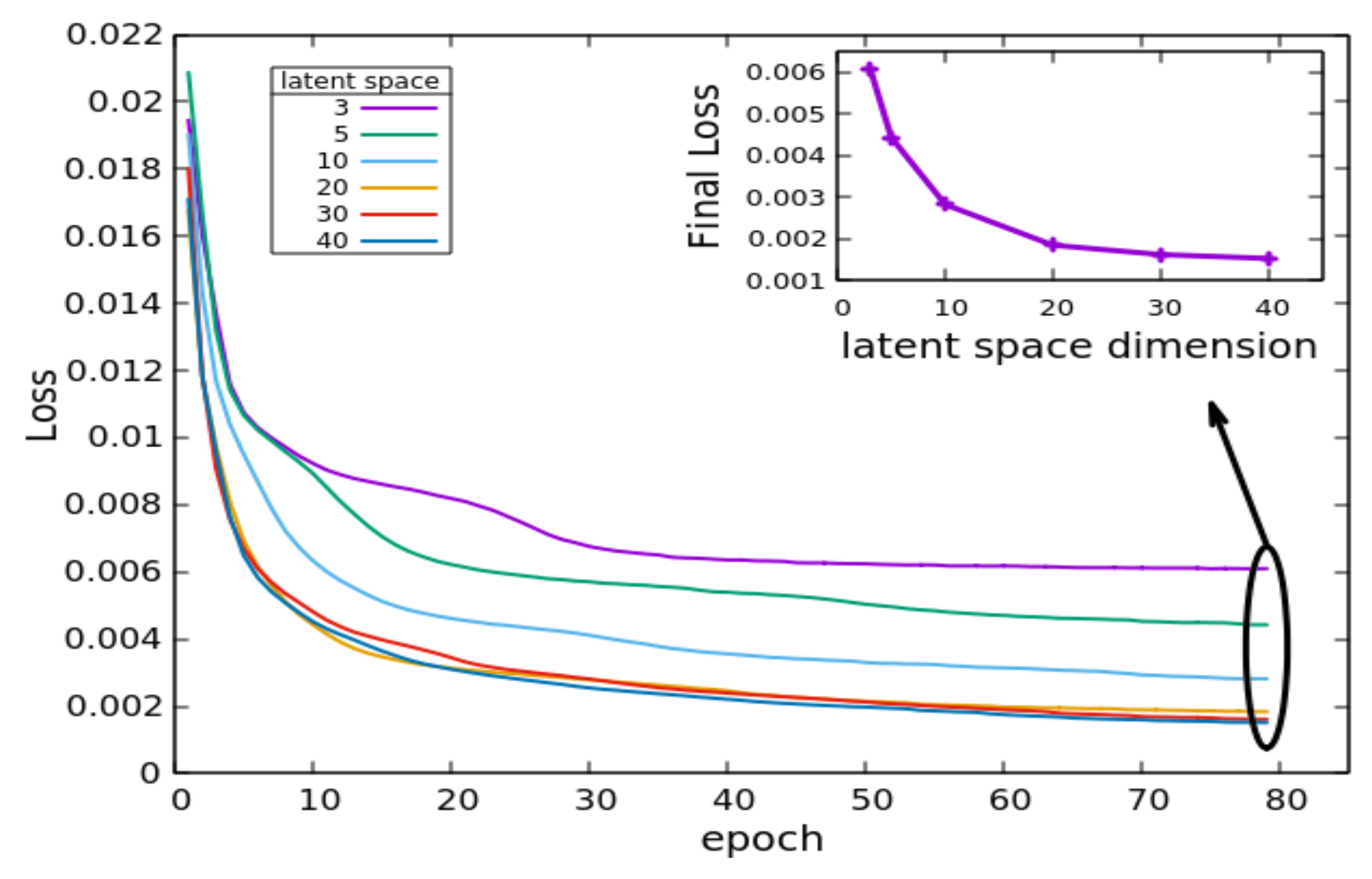
Several latent space dimensions were tested. Figure 3 summarizes both the training loss as a function of the training epochs and, in the inset, the final loss. It is evident that the larger the number of latent space units, the smaller the loss. For further processing, the latent space dimension was set to 20, since the gain in terms of loss using larger latent space dimensions is limited, while the smaller the number of units is, the more manageable the model and the related processing timings are.
4. Results
4.1. Generation
Once trained, the system was used for its true purpose: the generation of new trajectories for synthetic cars and drivers.
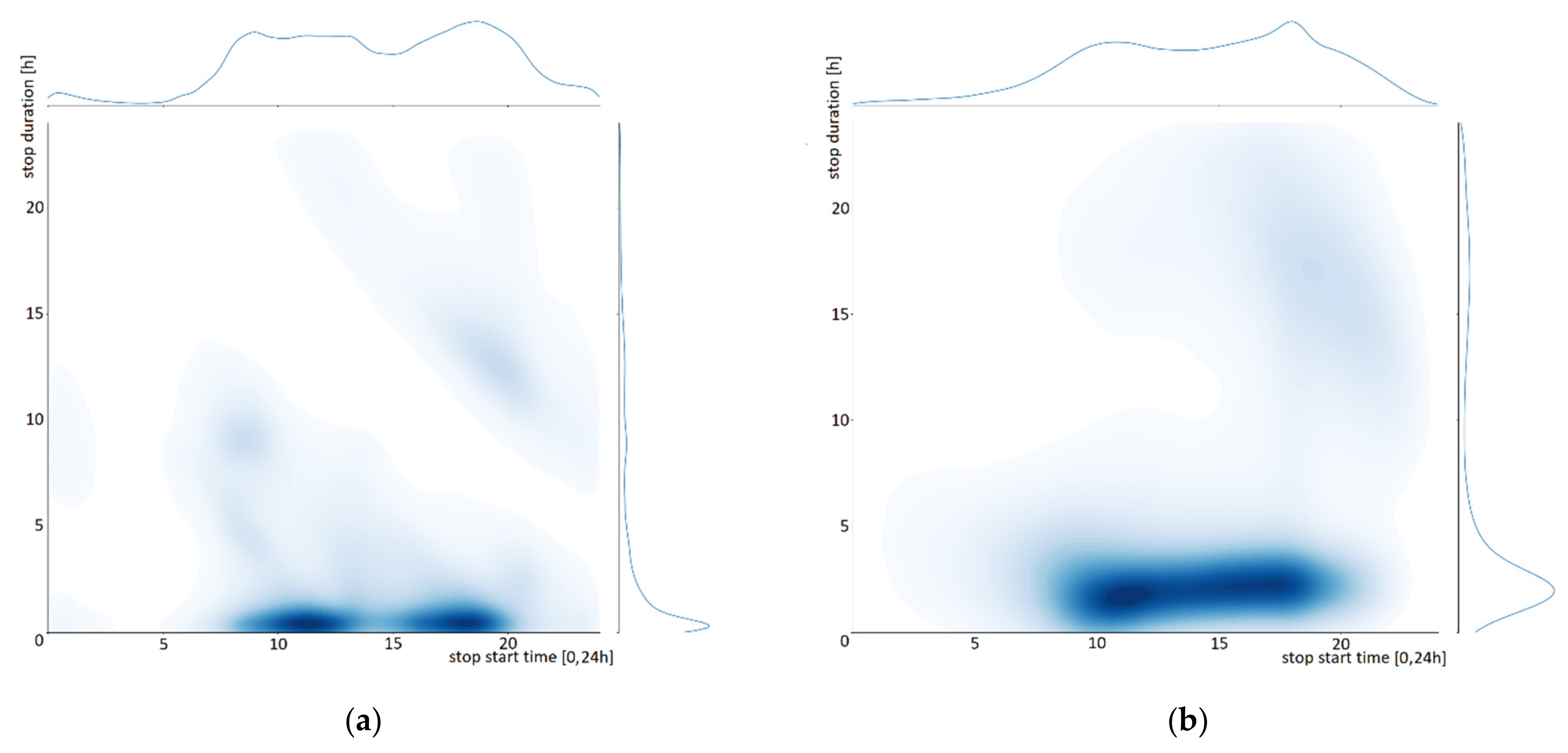
In Figure 4, the same bivariate histogram of Figure 1 is presented, i.e., stop start time versus stop duration.
The original training dataset is on the left of the figure, and the generated trajectories are on the right. The short-term stops are in the same time slots and with slightly longer durations. The nightly stops in the generated trajectories are present, but they are somewhat longer in duration and are later in their beginning. Nevertheless, there is an evident similarity between the two graphs, and the overall quality of the generated trajectories is similar to the original dataset behavior.
The resulting generated trajectories were evaluated in terms of the extent to which the synthetic generated data retain the features of the real data. Specifically, the consistency of the number of stops, the trip distance distribution, and the time spent per location (stop duration) was checked. It is important to mention that it is difficult to compare output from other studies because different algorithms have different aims and different datasets.
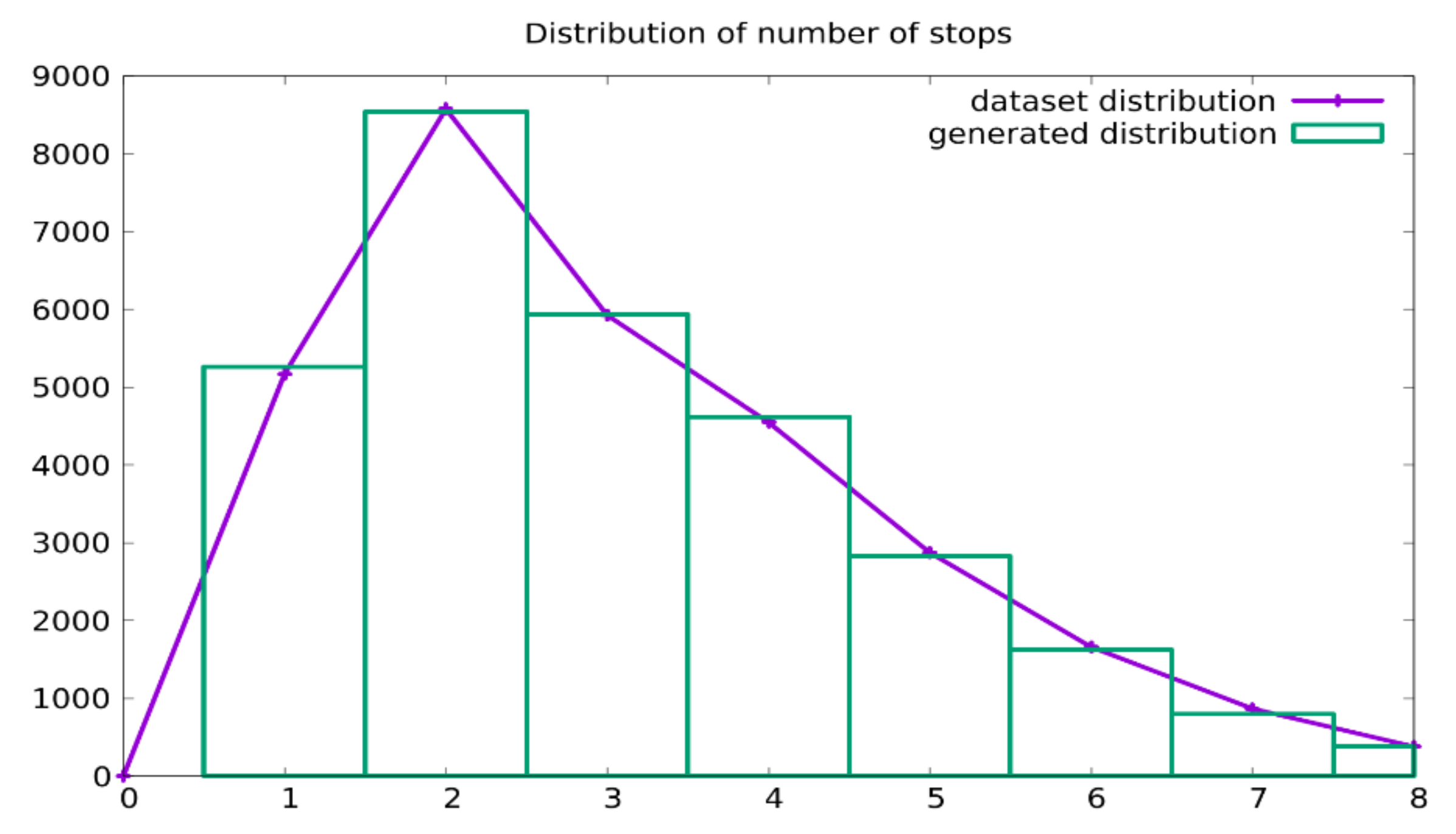
In Figure 5, the distribution of the number of daily stops, in both the training dataset and the generated trajectories, is presented. The solid line represents the dataset, while the histogram shows the generated data. The comparison shows that the statistical distribution of this quantity was grasped by the generative model.
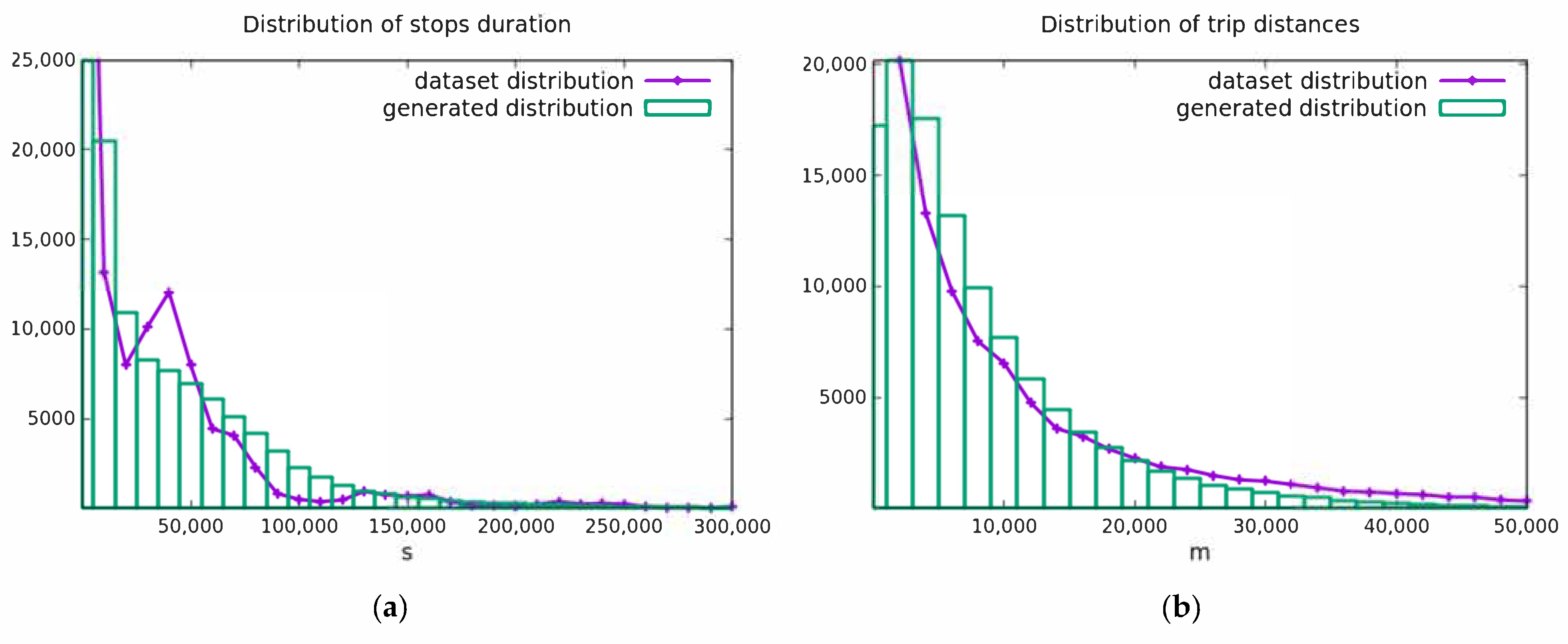
The distribution of stop durations is shown in Figure 6a. The solid line is the dataset, while the histogram describes the generated data. In this case, the overall distribution pattern is grasped by the modeling VAE, but with a lower accuracy. In Figure 6b, the distribution of the trip distances is shown. Here, the generative model resembles the dataset distribution with a higher degree of accuracy.
4.2. Reconstruction
Although the generated data possess general descriptors similar to the training data as described above, the actual geographic distribution of the generated stops is not adequate for the purpose of an accurate model of the traffic request.
In order to overcome this limitation, it can be observed that, in addition to the generative mode, it is also possible to use the autoencoder to reconstruct the training dataset. If the training dataset is fed as input, the reconstructed trajectories in the output will be statistically similar but not equal to those of the dataset itself, yielding a different possibility for traffic modeling. The trained VAE was made thus to reconstruct the input data. The results were compared in terms of Kullback–Leibler divergence with the input data distribution. The reconstruction performs better than the generation (see Table 2).
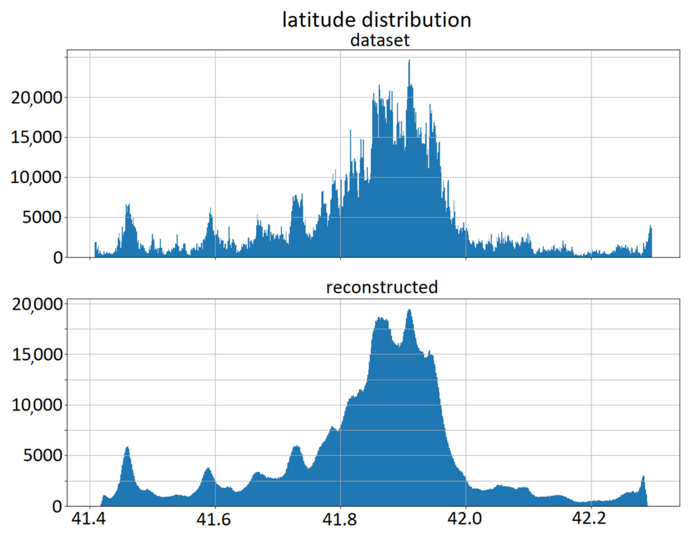
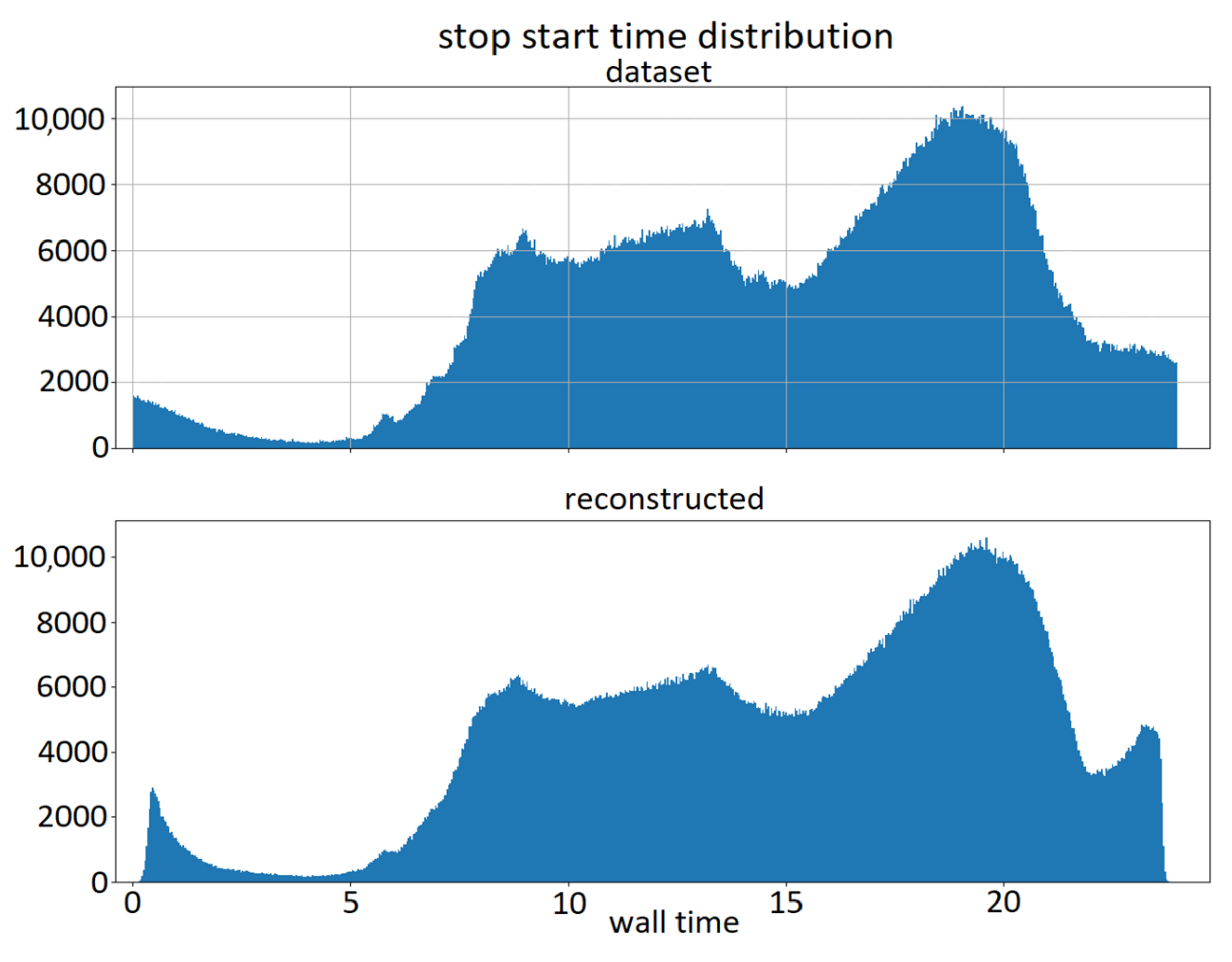
In Figure 7 and Figure 8, the reconstructed data for latitude and stop starting time are shown. The upper plot represents the dataset distribution, and the lower plot represents the reconstructed distribution. Similar plots were obtained for the other relevant quantities of the model. As can be seen from the juxtaposed plots, the obtained distributions are similar to the original ones; however, they still possess an intrinsic stochastic variability due to the use of the VAE architecture. This allows for the production of more data than those in the training set if needed, though with the same overall distribution.
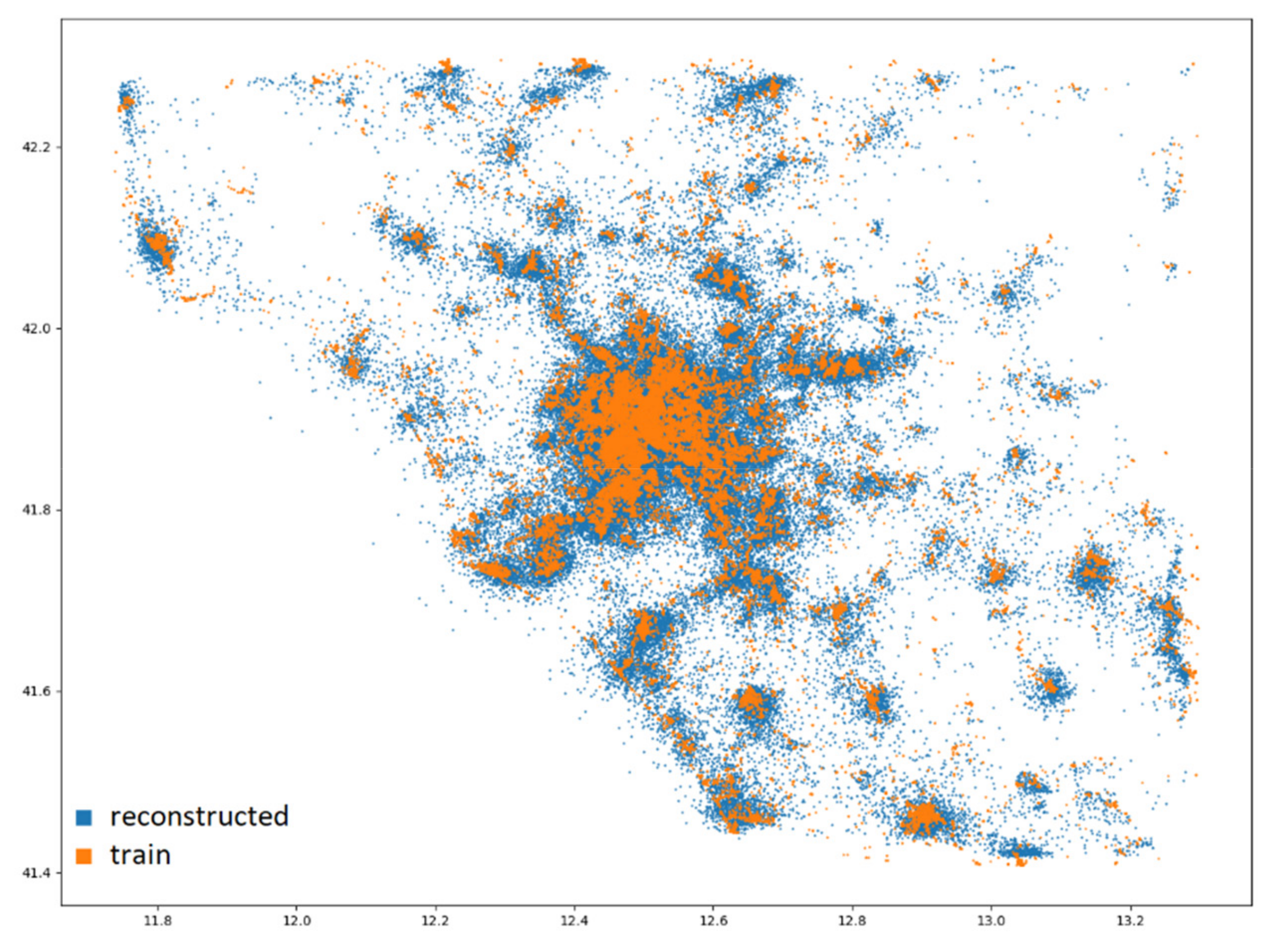
In Figure 9, the geographic locations of the first 30,000 stops are plotted to avoid clutter. The distribution of the dataset is in orange, and the reconstructed data are in blue.
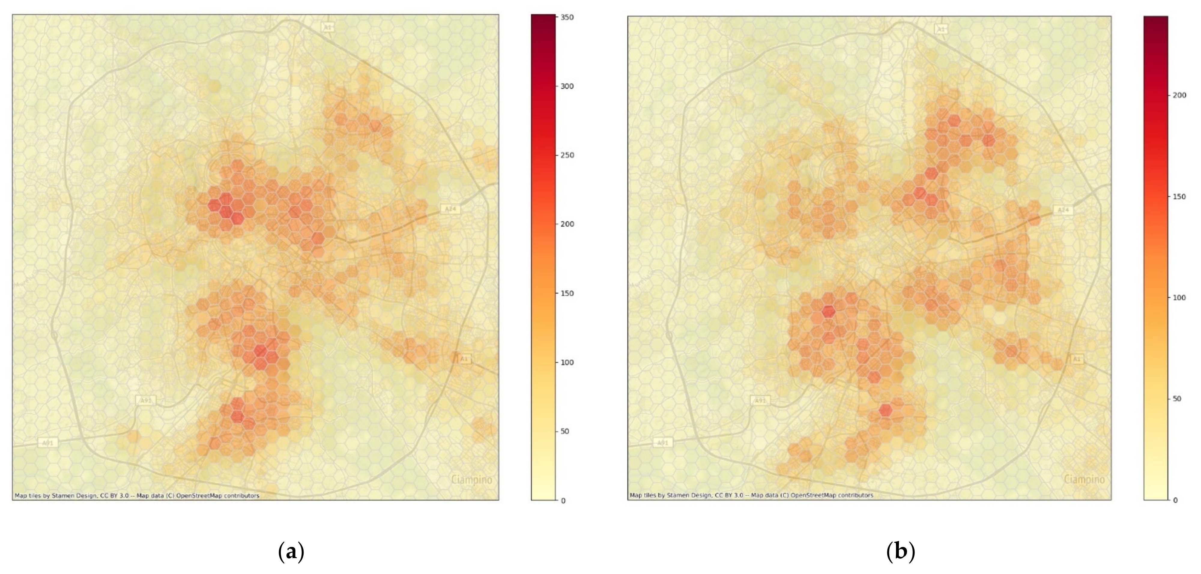
Once the model was used to generate the traffic demand in the city, the origin-destination matrices were computed, and examples of the results in terms of traffic fluxes are visualized in Figure 10 and Figure 11 for the time slot between 9 and 10 a.m. on a weekday.
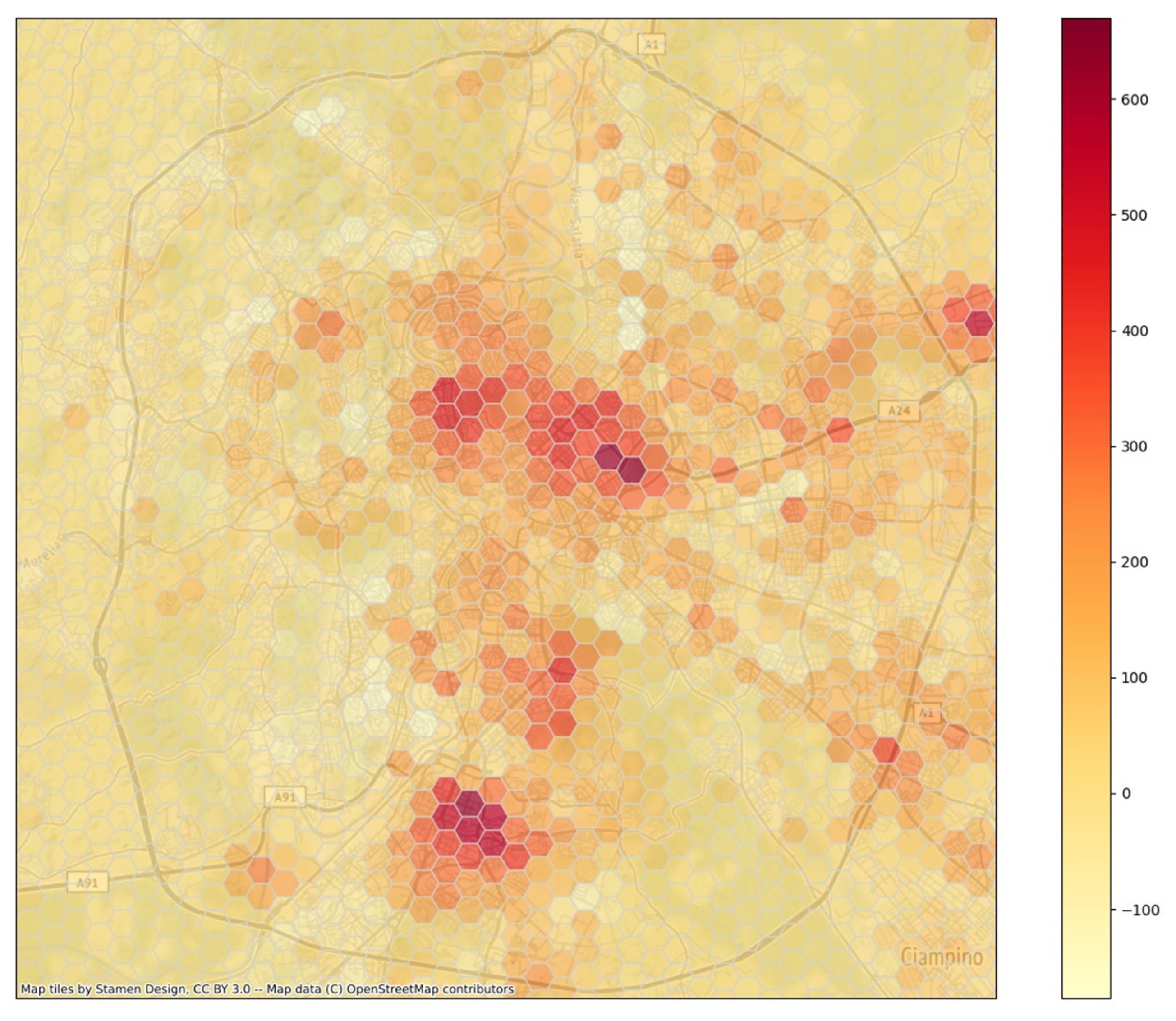
Figure 10 shows the inbound and outbound car flows, as discretized using about 17,000 hexagons with a diagonal of 700 m. Figure 11 plots the resulting parked cars under the assumption of an initial number of parked cars distributed in the city as computed residences, i.e., the overnight stops of at least 8 h.
In the figures, the beltway around Rome and the districts where the working places are more densely located can be seen, i.e., in the lower part of the city and in the upper part of the center. In addition, an industrial area is visible outside the beltway on the upper right part.
5. Discussion and Conclusions
The generation of urban traffic patterns is needed to secure a greener and more sustainable environment to the citizens. This task involves the processing of large quantities of data, typically collected from mobile phones or car navigational tools, which has implications in terms of residents’ privacy and, in a data availability issue, often these datasets are a limited or biased sample of the population.
Aiming to generate traffic patterns and avoid violations of privacy, a variational autoencoder generative model, based on dense neural networks, is presented. The dataset employed to train the system is an FCD, which was translated into stop-trajectories, i.e., sequences of stops with associated locations and time information. This approach can be approximately considered activity-based [3], even if this is not entirely accurate as compared to the use of mobile phones data. At the same time, it differs from the full trajectory approach, where the full collection of locations along the trajectory are considered as in [9,14].
The stop trajectories are here limited to eight stops out of statistical considerations on the actual dataset. Thus, the use of a dense VAE model considering daily stop trajectories, instead of a recurrent network reconstructing trajectory points sequences, as done in [14,15], is viable.
The locations considered here are expressed in terms of latitude–longitude pairs, differently from other works, e.g., [15], where census tract areas are used. In [16], deviations of the latitudes and longitudes from the centroid of all latitudes and longitudes are used instead.
An interesting issue is that of the comparison of distribution features between synthetic and real data. In the case of pure generation, the model is able to grasp and reproduce feature distributions in acceptable accordance, but the spatial distribution somehow becomes insufficiently accurate for the needed application.
The reconstructed stop-trajectories can more accurately describe the real data. This method is in some sense similar to the approach in [15], where home and work locations are used as seeds to reconstruct a complete daily trajectory.
The use of a generative model automatically ensures the the data abundance issue is overcome. Under the perspective of privacy, it is possible to affirm that the stop trajectory data produced by the model is synthetic and loosely linked to the original dataset, but it is obvious that the training of the model is performed using real data. Future work will be focused on an evaluation of the privacy issues using distance metrics to compare synthetic trajectories and real ones from the original dataset, as in [15].
Further work will also be aimed at checking the approach with a tiling technique for geographic localization, as in Figure 10 and Figure 11, since the goal of this work is to model traffic needs in terms of origin–destination matrices. Validation of these future implementations will be performed against different, larger, and more recent traffic datasets.
Author Contributions
Authors equally contributed to this work. All authors have read and agreed to the published version of the manuscript.
Funding
This work has been partially funded by the Italian Ministry of Ecologic Transition in the framework of the Triennial Plan 2019–2021 of the National Research on the Electrical System (Piano Triennale 2019–2021 della Ricerca di Sistema Elettrico Nazionale).
Institutional Review Board Statement
Not applicable.
Informed Consent Statement
Not applicable.
Data Availability Statement
Restrictions apply to the availability of these data. Data were obtained from OCTO Telematics Italia s.r.l.
Acknowledgments
The authors sincerely thank the editor and the anonymous reviewers for constructive comments and suggestions to clarify the content of the paper. The authors are indebted to Gaetano Valenti for discussions on traffic modeling and ride-sharing related issues.
Conflicts of Interest
The authors declare that there is no conflict of interest.
References
- Zheng, Y.; Capra, L.; Wolfson, O.; Yang, H. Urban computing: Concepts, methodologies, and applications. ACM Trans. Intell. Sys. Technol. 2014, 5, 38. [Google Scholar] [CrossRef]
- Qiao, F.; Liu, T.; Sun, H.; Guo, L.; Chen, Y. Modelling and simulation of urban traffic systems: Present and future. Int. J. Cybern. Cyber Phys. Sys. 2021, 1, 1–32. [Google Scholar] [CrossRef]
- Chu, Z.; Cheng, L.; Chen, H. A Review of Activity-Based Travel Demand Modeling. In Proceedings of the Twelfth COTA International Conference of Transportation Professionals, Beijing, China, 3–6 August 2012; pp. 48–59. [Google Scholar] [CrossRef]
- Gonzalez, M.C.; Hidalgo, C.A.; Barabasi, A.L. Understanding individual human mobility patterns. Nature 2008, 453, 779–782. [Google Scholar] [CrossRef] [PubMed]
- Song, C.; Qu, Z.; Blumm, N.; Barabasi, A.L. Limits of predictability in human mobility. Science 2010, 327, 1018–1021. [Google Scholar] [CrossRef] [PubMed] [Green Version]
- Alessandretti, L.; Sapiezynski, P.; Lehmann, S.; Baronchelli, A. Evidence for a Conserved Quantity in Human Mobility. Nat. Hum. Behav. 2018, 2, 485–491. [Google Scholar] [CrossRef] [PubMed]
- Keβler, C.; McKenzie, G. A geoprivacy manifesto. Trans. GIS 2018, 22, 3–19. [Google Scholar] [CrossRef] [Green Version]
- Harshvardhan, G.M.; Gourisaria, M.K.; Pandey, M.; Rautaray, S.S. A comprehensive survey and analysis of generative models in machine learning. Comput. Sci. Rev. 2020, 38, 100285. [Google Scholar] [CrossRef]
- Yin, M.; Sheehan, M.; Feygin, S.; Paiement, J.; Pozdnoukhov, A. A Generative Model of Urban Activities from Cellular Data. IEEE Trans. Intel. Transp. Sys. 2018, 19, 1682–1696. [Google Scholar] [CrossRef]
- Lin, Z.; Yin, M.; Feygin, S.; Sheehan, M.; Paiement, J.F.; Pozdnoukhov, A. Deep Generative Models of Urban Mobility. In Proceedings of the KDD’17, Halifax, NS, Canada, 13–17 August 2017. [Google Scholar]
- Anda, C.; Ordonez Medina, S.A. Privacy-by-design generative models of urban mobility. Arb. Verk. Raumplan. 2019, 1454. [Google Scholar] [CrossRef]
- Pappalardo, L.; Simini, F. Data-driven generation of spatio-temporal routines in human mobility. Data Min. Knowl. Discov. 2018, 32, 787–829. [Google Scholar] [CrossRef] [PubMed] [Green Version]
- Goodfellow, I.; Pouget-Abadie, J.; Mirza, M.; Xu, B.; Warde-Farley, D.; Ozair, S.; Courville, A.; Bengio, Y. Generative adversarial networks. Commun. ACM 2020, 63, 139–144. [Google Scholar] [CrossRef]
- Huang, D.; Song, X.; Fan, Z.; Jiang, R.; Shibasaki, R.; Zhang, Y.; Wang, H.; Kato, Y. A Variational Autoencoder Based Generative Model of Urban Human Mobility. In Proceedings of the 2019 IEEE Conference on Multimedia Information Processing and Retrieval (MIPR), San Jose, CA, USA, 28–30 March 2019; pp. 425–430. [Google Scholar] [CrossRef]
- Berke, A.; Doorley, R.; Larson, K.; Moro, E. Generating synthetic mobility data for a realistic population with RNNs to improve utility and privacy. arXiv 2022, arXiv:2201.01139. [Google Scholar] [CrossRef]
- Rao, J.; Gao, S.; Kang, Y.; Huang, Q. LSTM-TrajGAN: A Deep Learning Approach to Trajectory Privacy Protection. In Proceedings of the 11th International Conference on Geographic Information Science, GIScience (2021), Poznań, Poland, 27–30 September 2021. [CrossRef]
- Ouyang, K.; Shokri, R.; Rosenblum, D.S.; Yang, W. A Non-Parametric Generative Model for Human Trajectories. In Proceedings of the Twenty-Seventh International Joint Conference on Artificial Intelligence, IJCAI-18, Stockholm, Sweden, 9–19 July 2018; pp. 3812–3817. [Google Scholar] [CrossRef] [Green Version]
- Chiesa, S.; Taraglio, S. Traffic modelling through a LSTM variational auto encoder approach: Preliminary results. In Computational Science and Its Applications—ICCSA 2021. Lecture Notes in Computer Science LNCS 12950, Proceedings of the ICSSA 2021, Cagliari, 13–16 September 2021; Gervasi, O., Murgante, B., Misra, S., Garau, C., Blečić, I., Taniar, D., Apduhan, B.O., Rocha, A.M.A.C., Tarantino, E., Torre, C.M., Eds.; Springer: Cham, Switzerland, 2021; pp. 598–606. [Google Scholar] [CrossRef]
- Hochreiter, S.; Schmidhuber, J. Long Short-Term Memory. Neural Comput. 1997, 9, 1735–1780. [Google Scholar] [CrossRef] [PubMed]
- Chollet, F. Deep Learning with Python; Manning Pub Co.: Shelter Island, NY, USA, 2018; Chapter 6. [Google Scholar]
- OCTO Telematics Italia s.r.l. Available online: https://www.octotelematics.com/it/home-it/ (accessed on 30 March 2022).
Figure 1.
Bivariate histogram of the stops on a weekday. The x axis is the starting time of the stops, and the y axis is the relative duration, both in hours. The red dotted lines delimit the day. The intensity of color increases with the number of stops. On the right side and on the top of the graph are the two monovariate distributions.

Figure 2.
Final loss behavior as a function of the trade-off parameter β between the reconstruction error (MSE) and the regularization term (KL). A value of β around 0.2 assures a low MSE with good regularization.
Figure 2.
Final loss behavior as a function of the trade-off parameter β between the reconstruction error (MSE) and the regularization term (KL). A value of β around 0.2 assures a low MSE with good regularization.

Figure 3.
Training with different latent space dimensions. Larger graph: The total loss as a function of training epochs for different latent space dimensions. Inset: The final loss behavior as a function of latent space dimension (β = 0.2).
Figure 3.
Training with different latent space dimensions. Larger graph: The total loss as a function of training epochs for different latent space dimensions. Inset: The final loss behavior as a function of latent space dimension (β = 0.2).

Figure 4.
Histograms of the stop start time vs. duration: (a) the training dataset; (b) the generated trajectories.
Figure 4.
Histograms of the stop start time vs. duration: (a) the training dataset; (b) the generated trajectories.

Figure 5.
The distribution of the number of stops in the trajectories: comparison between that from the training dataset (line) and that from the generated trajectories (histogram).
Figure 5.
The distribution of the number of stops in the trajectories: comparison between that from the training dataset (line) and that from the generated trajectories (histogram).

Figure 6.
(a) The distribution of stop duration: training dataset (line) and generated trajectories (histogram); (b) the distribution of trip distances: training dataset (line) and generated trajectories (histogram).
Figure 6.
(a) The distribution of stop duration: training dataset (line) and generated trajectories (histogram); (b) the distribution of trip distances: training dataset (line) and generated trajectories (histogram).

Figure 7.
Latitude data comparison. Above: dataset distribution; below: reconstructed distribution.

Figure 8.
Stop starting hour comparison. Above: dataset distribution; below: reconstructed distribution.
Figure 8.
Stop starting hour comparison. Above: dataset distribution; below: reconstructed distribution.

Figure 9.
Spatial distribution (latitude; longitude) of the first 30,000 stops. Orange: the dataset; blue: the reconstructed data.
Figure 9.
Spatial distribution (latitude; longitude) of the first 30,000 stops. Orange: the dataset; blue: the reconstructed data.

Figure 10.
Hexagon aggregated fluxes: (a) Inbound cars and (b) outbound ones between 8 and 9 a.m. on a weekday.
Figure 10.
Hexagon aggregated fluxes: (a) Inbound cars and (b) outbound ones between 8 and 9 a.m. on a weekday.

Figure 11.
Parked cars between 8 and 9 a.m. on a weekday.


Table 1.
An example of a stop-trajectory: eight stops, possibly zero padded, described by six values. A five-stop trajectory is shown here. Start time is in decimal hours. In this case, the first stop is in the preceding day, with a duration of circa 12 h.
Table 1.
An example of a stop-trajectory: eight stops, possibly zero padded, described by six values. A five-stop trajectory is shown here. Start time is in decimal hours. In this case, the first stop is in the preceding day, with a duration of circa 12 h.
| Latitude | Longitude | Duration (s) | Start Time (h) | Day of Week | Trip Distance (m) | |
|---|---|---|---|---|---|---|
| 1 | 41.854031 | 12.497663 | 43,406.00 | 20.266 | 3 | 6035.0 |
| 2 | 41.844841 | 12.490471 | 16,362.00 | 8.433 | 4 | 1580.0 |
| 3 | 41.829877 | 12.510948 | 411.00 | 13.149 | 4 | 3606.0 |
| 4 | 41.853169 | 12.497894 | 4363.00 | 13.516 | 4 | 5553.0 |
| 5 | 41.852843 | 12.498169 | 57,320.99 | 14.933 | 4 | 4348.0 |
| 6 | 0 | 0 | 0 | 0 | 0 | 0 |
| 7 | 0 | 0 | 0 | 0 | 0 | 0 |
| 8 | 0 | 0 | 0 | 0 | 0 | 0 |
Table 2.
Kullback–Leibler divergence between the input data and the generated or reconstructed output (a null divergence means that the two distributions are equal).
Table 2.
Kullback–Leibler divergence between the input data and the generated or reconstructed output (a null divergence means that the two distributions are equal).
| Variable | Generated Data | Reconstructed Data |
|---|---|---|
| Latitude | 4.44 × 10⁻⁴ | 2.03 × 10⁻⁴ |
| Longitude | 1.56 × 10⁻⁴ | 9.21 × 10⁻⁵ |
| Duration | 8.30 × 10⁻⁵ | 7.79 × 10⁻⁵ |
| Trip Distance | 3.46 × 10⁻³ | 2.68 × 10⁻³ |
Publisher’s Note: MDPI stays neutral with regard to jurisdictional claims in published maps and institutional affiliations. |
© 2022 by the authors. Licensee MDPI, Basel, Switzerland. This article is an open access article distributed under the terms and conditions of the Creative Commons Attribution (CC BY) license (https://creativecommons.org/licenses/by/4.0/).
Share and Cite
MDPI and ACS Style
Chiesa, S.; Taraglio, S. Traffic Request Generation through a Variational Auto Encoder Approach. Computers 2022, 11, 71. https://0-doi-org.brum.beds.ac.uk/10.3390/computers11050071
AMA Style
Chiesa S, Taraglio S. Traffic Request Generation through a Variational Auto Encoder Approach. Computers. 2022; 11(5):71. https://0-doi-org.brum.beds.ac.uk/10.3390/computers11050071
Chicago/Turabian StyleChiesa, Stefano, and Sergio Taraglio. 2022. "Traffic Request Generation through a Variational Auto Encoder Approach" Computers 11, no. 5: 71. https://0-doi-org.brum.beds.ac.uk/10.3390/computers11050071
Note that from the first issue of 2016, this journal uses article numbers instead of page numbers. See further details here.