
A Highly Adaptive Oversampling Approach to Address the Issue of Data Imbalance


Faculty of Informatics, University of Debrecen, H-4032 Debrecen, Hungary
*
Author to whom correspondence should be addressed.
Computers 2022, 11(5), 73; https://0-doi-org.brum.beds.ac.uk/10.3390/computers11050073
Submission received: 22 February 2022
/
Revised: 22 April 2022
/
Accepted: 27 April 2022
/
Published: 4 May 2022
Abstract
:Data imbalance is a serious problem in machine learning that can be alleviated at the data level by balancing the class distribution with sampling. In the last decade, several sampling methods have been published to address the shortcomings of the initial ones, such as noise sensitivity and incorrect neighbor selection. Based on the review of the literature, it has become clear to us that the algorithms achieve varying performance on different data sets. In this paper, we present a new oversampler that has been developed based on the key steps and sampling strategies identified by analyzing dozens of existing methods and that can be fitted to various data sets through an optimization process. Experiments were performed on a number of data sets, which show that the proposed method had a similar or better effect on the performance of SVM, DTree, kNN and MLP classifiers compared with other well-known samplers found in the literature. The results were also confirmed by statistical tests.
1. Introduction
Classification is a typical machine-learning task that aims to classify set of samples into predefined classes. Each sample represents a given entity with d observed features. More formally, if the samples belong to k different classes (labeled ), the goal is to build a model based on a sample set and their corresponding class labels , where , , which can be used to predict a class label of an sample. The set of samples and their corresponding labels used to build the model are called a training data set. If there are only two classes (), then the problem is a binary classification problem. If the size of the classes differs significantly, the set containing all the samples of the smaller class is called the minority set, and the set containing all the samples of the larger class is called the majority set.
The classical classification algorithms, such as the Naive Bayes, linear SVM and Random Trees, were designed for balanced data sets. If the class distribution is uneven, the models built on the data set usually favor the larger class. Data imbalance must also be taken into account in model evaluation as an inappropriate metric may provide a completely misleading result about the performance of a classifier [1].
We can easily understand the problem by imagining a simple classification task where the samples, represented by triangles and circles, have to be classified into the Triangle class and the Circle class, respectively. The training data set that can be used to build the model has 1000 samples, 990 circles and only 10 triangles. If we consider a trivial classifier that predicts the Circle label for each sample, it would make a good decision for 99% of the samples in the data set; however, in practice, the classifier is completely useless.
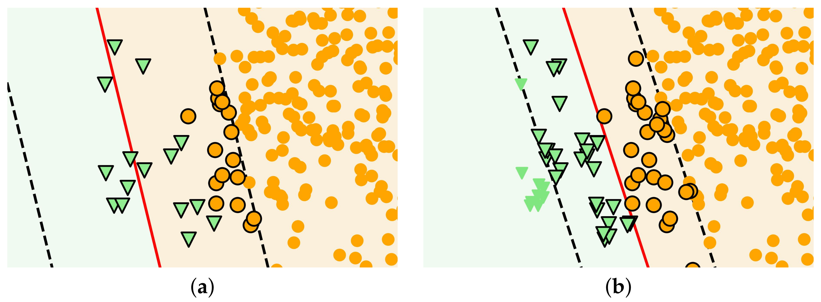
A less extreme example is shown in Figure 1a. We built a model with a linear SVM on the data set with 200 circles and 15 triangles. The red line indicates the decision boundary for separating samples belonging to different classes. If a sample to be classified falls to the left of the red line, the classifier will classify it as a triangle—otherwise, as a circle. One can readily see that the location of the decision boundary favors the classification of circles to the detriment of triangles. However, on a less imbalanced version of the data set, the classifier was able to find a good decision boundary (Figure 1b).
We can also observe in Figure 1 that the samples far from the decision boundary can be classified correctly even by the worse classifier. These easily classifiable samples are commonly referred to as safe samples. However, some of the samples near the boundary would be classified differently based on the two models. These samples may play an important role in the construction of the model; however, they are in danger of misclassification as they are very similar to some samples of the other class.
Imbalanced learning has been a focus of interest for two decades, and there are several learning problems in practice where the distribution of classes is skewed (e.g., spam filtering [2], fault detection [3,4], disease risk prediction [5], cancer diagnosis [6], dynamic gesture recognition [7,8], activity monitoring [9] and online activity learning [10]).
We can handle the problem of imbalanced data at the algorithm level, whose best-known representatives are perhaps the cost-sensitive methods. The concept behind them is simple, the misclassification of minority samples costs more (entails a higher penalty) than the misclassification of majority ones [11]. If large amounts of imbalanced data need to be classified, the use of some cost-sensitive deep-learning methods should also be considered [12].
In contrast to the previous approach, data-level algorithms address the root of the problem by changing the number and/or distribution of data before applying general classifiers. For binary classification problems, this can be accomplished by oversampling the smaller class or undersampling the larger one, and hybrid solutions also exist that combine under- and oversampling [1,13]. All three approaches can also be found in the field of deep learning to handle large amounts of imbalanced data [14].
One of the advantages of oversampling is that it preserves the information in the data. In addition, oversampling usually reduces the proportion of samples that are difficult to classify and increases the proportion of the safe samples in the data set, while undersampling tends to remove safe samples from the data set preserving the samples that are difficult to classify. This means that the classification with oversampled data sets is likely to be more efficient than using undersampled ones [15].
In the rest of this paper, we focus primarily on the oversampling algorithms (excluding deep-learning-based solutions). Of the many oversampling algorithms in the literature, it is perhaps worth highlighting that, historically, the algorithm of SMOTE released in 2002 [16]. The SMOTE attempts to add synthetic samples to the minority set that are similar to but not duplicates of the minority samples.
To achieve this goal, each synthetic sample is generated by interpolating a randomly selected minority sample (seed) and one of its k nearest minority neighbors (co-seed and pair). We can already see the advantage of using SMOTE because the original Circle–Triangle data set (Figure 1a) was oversampled by SMOTE to make a more balanced version (Figure 1b).
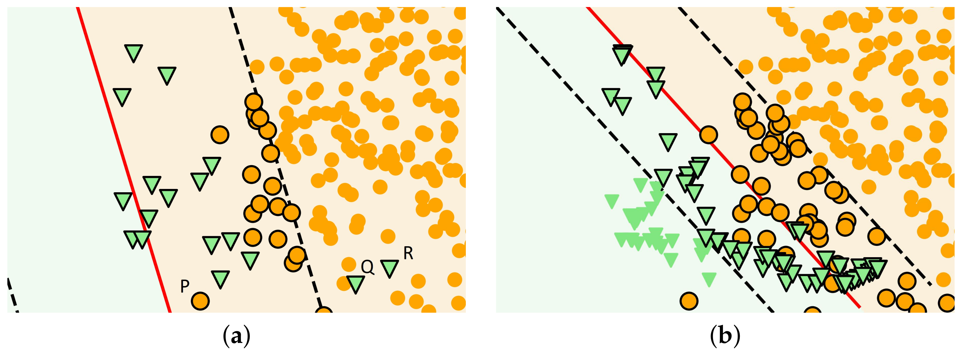
Nevertheless, SMOTE also has certain disadvantages: it selects samples as seeds that are important (e.g., a sample close to the decision boundary), irrelevant (e.g., a sample far to the decision boundary) and misleading (e.g., noise) for classification with equal probability, and the situation is similar for the selection of co-seeds. To provide a clear picture of the problem, we have supplemented the Circle–Triangle data set with three noise samples denoted by P, Q and R (Figure 2a), and then the data set was oversampled by SMOTE to a similar extent as before.
If we compare Figure 1a to Figure 2a, we can see that the decision boundary has shifted due to noise. Furthermore, Figure 2b shows, that, as a result of oversampling, plenty of new samples appeared around Q and R, thus, increasing the degree of overlap between classes. Moreover, these samples misled the classifier, because they belong to the Triangle class but they are similar to circles.
Over the years, more than a hundred SMOTE variants have been published to overcome the drawbacks of the original version. The interested reader can find more about the SMOTE algorithm, including the several variants in an excellent summary in the literature [17]. It covers current challenges, such as handling streamed data or using semi-supervised learning.
The following section provides a brief overview of oversampling methods. Then, in Section 3, we introduce our ModularOverSampler, which was designed taking into account the common features and differences of the methods found in the literature. Section 4 provides a detailed description of the experimental process and the results. In Section 5, we discuss the limitations of our method and suggest some directions for further research. Finally, conclusions are drawn in Section 6.
2. Related Work
Although there are plenty of oversamplers that have been published in the literature, the theoretical considerations behind them, often based on a priori assumptions, serve the same purpose—to ensure that the distribution and locations of the generated samples are adequate to improve the samples classification. A rough structural pattern is also recognizable in a fairly large proportion of the published algorithms; however, by further refining the structure, the diversity of the procedures becomes visible. During the review of the literature, we present the possible structural steps and their role, mentioning some typical implementation methods (strategies) as this supports our concept, which is described in a later section.
Some of the oversamplers start with noise filtering to permanently remove samples considered to be noise from the data set [18,19]. Using the filtered data set, we may obtain a clearer picture of which samples are at the decision boundary, where minority samples are in danger of misclassification. However, a noise filter is rarely applied to the minority set, because there is a danger that too many minority samples will be removed, thereby, increasing the degree of imbalance.
In addition, the minority set sometimes really consists of only a few samples because there are problems where the event to be observed is rare (e.g., fault detection [3], bankruptcy prediction [20]). The deletion of samples is only acceptable in very justified cases. For example, an isolated sample can be deleted from the minority class [18] if the overlap of classes is moderate. Samples representing noise and outliers can also be deleted [19].
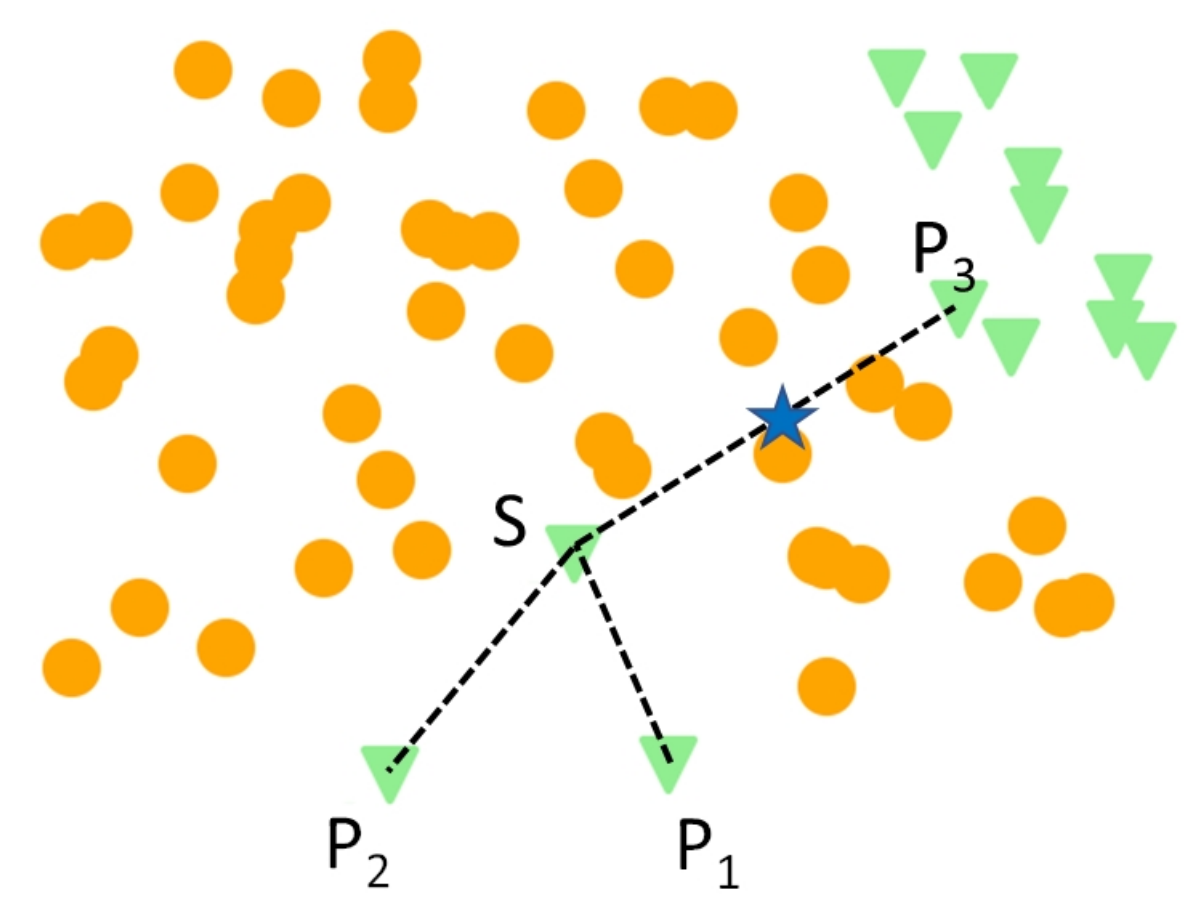
Another typical step is clustering [21], which can be used to delimit the part of the feature space where it is not worth generating samples. Placing the synthetic samples inside the clusters of the minority set helps to avoid the errors illustrated in Figure 3 [22]. The clustering also paves the way for distinguishing samples that are considered important or insignificant for the learning process.
For example, it may reveal the outliers and the isolated samples (possible noise samples), and thus we can exclude them from the further sampling process [23,24,25], and some procedures determine which samples are in danger of misclassification and which ones are safe based on the composition of the clusters, assuming that the decision boundary passes through clusters containing both minority and majority samples [26]. Instead of general-purpose clustering, many procedures determine the set of samples that are in danger, the set of the safe samples and the set of the noise samples based on the examination of the small environment of the samples (e.g., their k-nearest neighbors) [18,27,28,29].
Furthermore, with this, we have reached the next typical step, which is to weight the minority samples according to their importance. At this point, different approaches can be found in the literature because the assessment of the importance of samples varies from method to method. Some oversamplers consider all the minority samples equally important [20,30], while others exclude samples labeled for noise [24]. Contradictory strategies can also be found in algorithms.
For example, there are methods that assign a higher weight to samples near the decision boundary [31] than to samples that are far away (including the case where only boundary samples can become seeds [18]); however, for example, the Safe-Level-SMOTE generates samples near to the safe samples [32]. Furthermore, while many oversamplers ignore data samples in clusters that are too small, there is a method that assigns the largest weights to these minority samples assuming that they are not noises but rare samples [33].
The next step is to choose the seed samples. The selection is mostly made randomly from the samples of the minority set. The distribution of the selection can be uniform or weighted, as described in the previous paragraph.
The synthetic samples can be generated around the selected seeds [34,35]; however, most oversamplers select another sample (called a pair or co-seed) to each seed and create the new samples based on these samples. The most popular method to generate new samples is to interpolate the seeds and their pairs. Typically, the co-seeds are selected randomly from the k minority nearest neighbors of the seeds [20,23,36] or from the minority samples of the seeds cluster [37]. Although the seeds and their pairs are usually selected from the same cluster, borderline minority seeds can be strengthened if the new samples are created between them and the safe samples [38]. There are some methods that select the co-seeds from the majority set; however, this solution is not common [39].
Sample generation is not always the last step, while some methods reject samples generated in the wrong place during sample generation [26], others apply post-filtering on the oversampled data set [23,36,40]. The second strategy allows us to make a decision about removing or preserving the samples by seeing the modified version of the dataset that already includes the new synthetic samples. In this case, the sample removal is not limited to the newly generated samples.
3. Methodology
Researchers who require imbalanced data sets now have more than a hundred oversampling algorithms to choose from, and the increase in the number of samplers has not stopped in recent years. With this in mind, we have developed a new algorithm because it motivated us to create a generic sampler that can be well adapted to various databases.
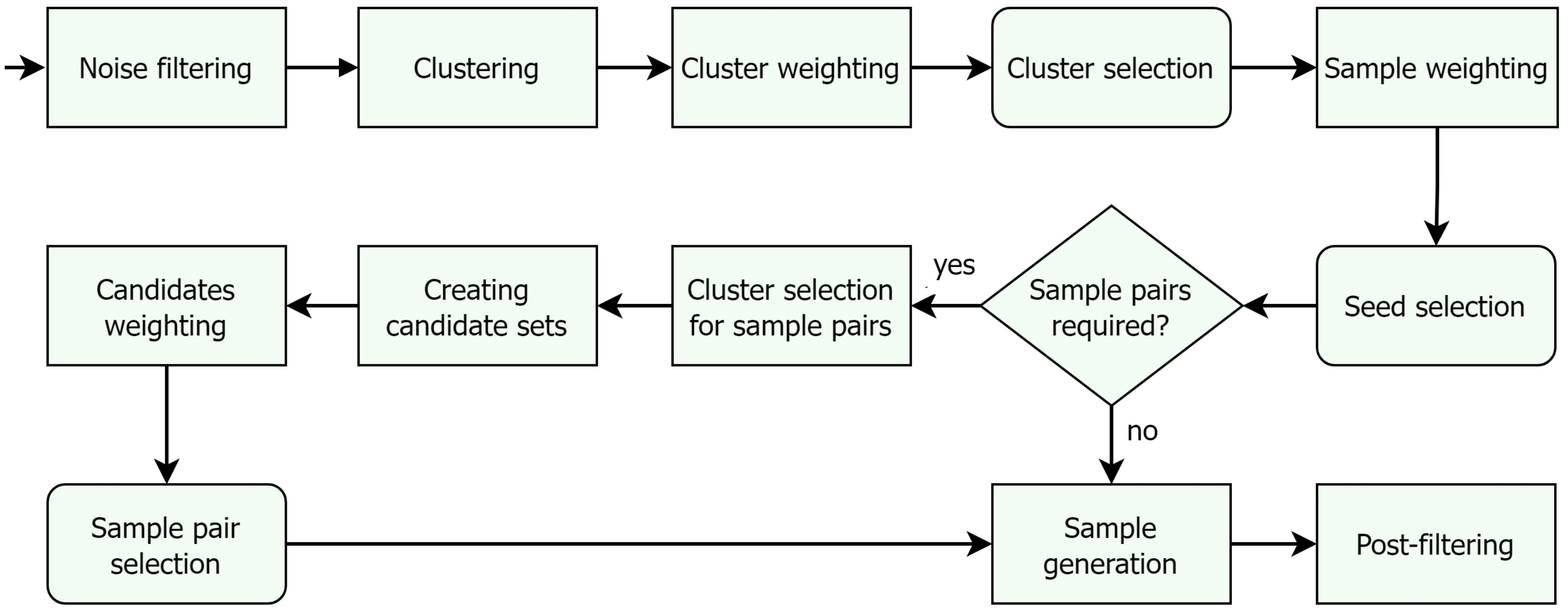
The proposed method utilizes many ideas from other samplers yet differs fundamentally from previously published solutions due to its modular structure. The main steps are shown in Figure 4. The method consists of a few more steps than we mentioned in the previous section because we have broken down certain steps into smaller ones for flexibility.
For most of the steps, we have defined different strategies which determine the specific methods of performing the steps. (These are described in detail later in this section). Our oversampler can be parameterized with these strategies. The non-round rectangles in Figure 4 indicate interchangeable modules that are swapped according to the strategies passed as parameters. This structure allows us to fundamentally modify the sampling process via parametrization.
Among the strategies, there are some that cannot be used together. The combination of parameters that assigns exactly one strategy to each interchangeable module and these strategies can be used together is called meaningful parameter combination or path. The algorithm is completed with an optimization step that selects the appropriate one from the paths for the data set to be sampled. We recommend cross-validation for this purpose.
3.1. Noise Filtering
As mentioned in Section 2, only a few methods attempt to remove the noise samples of the minority set permanently due to the risk of information loss. We also limited the noise removal to the majority set defining the noise with the Edited Nearest Neighbors (ENN) rule [30], which considers a sample as noise if the majority of its k-nearest neighbors (kNN) belong to another class. Similar solutions can be found in [41].
In this step, the noise removal algorithm can be used with and , and as a third option, we made it possible to skip the noise filtering step. We will refer to the three strategies as , and NoFilter.
3.2. Clustering
We mentioned in Section 2 that there may be different intentions behind the clustering step. Accordingly, the following strategies are defined:
- , : DBSCAN [42] applied on the minority set and the entire data set, respectively. DBSCAN does not require specifying the number of clusters in advance; it defines clusters with extensions starting from high-density points, where at least points must be within an distance. During the tests, was and was 3.
- BorderSafeNoise: With this strategy, a sample is placed to a NOISE cluster if there are at least samples with different labels among its 7 nearest neighbors, and a sample is added to the SAFE if there is no sample with different labels between its 7 nearest neighbors. All other samples form the BORDER cluster (). Similar solution can be found in [18].
- MinMaj: This strategy creates two clusters, the MINOR cluster includes all samples of the minority set, and the MAJOR cluster includes all samples of the majority set.
In the rest of the algorithm description, we denote the resulting clusters by S, the set of purely minority clusters by , the set of purely majority clusters by and the set of mixed clusters by . Furthermore, the size of cluster or set c are denoted by .
3.3. Cluster Weighting
In this step, the clusters can be given weight according to their importance. A normalized version of the weight of the cluster determines the probability of randomly selecting a seed from that cluster. For normalization, the weight of a cluster is divided by the sum of the weights of the clusters. By assigning zero weight, we can completely exclude clusters from the seed selection process. Four weighting strategies are defined: CW_Uniform, CW_BySize, CW_Border, CW_ByInsideEnemy. With the CW_Uniform strategy, we can assign the same positive weight to each cluster with at least one minority sample, creating the possibility that nearly the same number of seeds are selected from these clusters.
As a result, samples of the smaller clusters are expected to be involved in generating more synthetic samples than samples of the larger clusters, therefore, it reduces imbalance within the minority class but does not fully balance the clusters as the solution of Jo and Japkowicz [33]. The CW_BySize calculates the weight of clusters with at least one minority sample based on their size. More formally, the weight of a cluster is
All other clusters are given zero weight. If only pure clusters were generated in the previous step, this method ensures that all minority samples have the same chance of being selected as seed. If there are mixed clusters, their minority samples will have a higher chance of becoming a seed than the minority samples of other clusters. A similar solution can be found in [22]. (To avoid redundant paths, this weighting strategy is not used with the MinMaj clustering).
The CW_Border strategy assigns weight of 1 to the BORDER cluster and 0 to all others. As a result, only minority samples with a majority neighbor are selected as seeds. Clearly, this weighting only makes sense if BorderSafeNoise clustering was used in the previous step. The CW_ByInsideEnemy as its name implies, assigns high weight to the mixed clusters in which the number of majority samples is high relative to minority samples. Pure clusters receive zero weights.
For a , the weight is
This strategy is used only in combination with and BorderSafeNoise.
3.4. Cluster Selection
Using the normalized weights (probability values), we randomly select clusters by replacement. In a later step, we will select the seeds from these clusters. We attempted to achieve completely balanced classes, thus is the difference between the number of majority samples and the number of minority samples after the noise filtering step.
3.5. Sample Weighting
This step determines the probability of selecting a sample as a seed. Weighting is performed per cluster and majority samples are automatically given a weight of 0, therefore they cannot become seeds. After determining the weights of the samples, normalization is performed by dividing the weights by the total weight of the samples of their own cluster.
For this step, we defined two weighing strategies: SW_Uniform, SW_kNN.
With the SW_Uniform all minority samples within a cluster are given the same weight. If x is a minority sample of a c cluster, the weight assigned to it is
The SW_kNN follows in the footsteps of those samplers which attempt to create synthetic samples similar to those minority samples that are in danger for correct classification [18,31]. The danger level of a sample is often calculated based on the number of majority samples (enemies) among the sample’s k-nearest neighbors.
The variant used in this study determines the weight of a minority sample x according to the following formula:
where is the five nearest neighbors of x.
3.6. Seed Selection
To create a multiset of seed samples, we select as many samples from each cluster as the number of times the cluster was previously selected. The sample selection is made randomly with replacement based on the normalized weights (probabilities) that were calculated in the previous step.
3.7. Cluster Selection for Sample Pairs
As the flowchart shows, our oversampler supports sample generation based on a single sample (seed) and based on two samples (a seed and its pair). In the latter case, we need to select a cluster for each seed from which its pair can be selected. These clusters are called the cluster pair of seeds. We have defined the following strategies for this step.
CPM_MINOR: The least restrictive strategy, the MINOR cluster are the cluster pair of each seed.
CPM_SAFE: With this method the minority samples of the SAFE cluster are the cluster pairs of each seed. It can only be used in combination with BorderSafeNoise clustering. As a result, minority samples in danger of misclassification are associated with safe samples, and thus the generated synthetic samples can strengthen the position of the seeds without deteriorating the position of the majority samples around them [38].
CPM_SelfCluster: Using this method, the cluster pair of a seed is the set of minority samples of its own cluster, including the case when both the seed and its pair are taken from the BORDER cluster. This option was motivated by the SOI_C [22].
3.8. Creating Candidate Sets
The purpose of this step is to determine a set of pair candidates for each seed using the output of the previous step. In the simplest case (CS_ALL), we keep all the sample and the candidate set(s) is(are) the output of the previous step.
The second option, CS_kNN, covers a popular approach, when the pairs of the seeds are from the seeds’ nearest neighbors (See, e.g., SMOTE [16], Lee [43]). During the tests, the five nearest neighbors of a seed formed its candidate set, and the nearest neighbors were selected from the pair cluster of the seed.
The third option, CS_ClusterCenter, allows us to examine a less common solution where cluster centers are used in some way to create new synthetic samples (e.g., AHC [44], SMMO [45]). In our case, a candidate set assigned to a seed consists of a single artificial sample that represents the center of the cluster pair of the seed.
3.9. Candidate Weighting
At this point in the process, we assign weights to each sample of the candidate set(s) to determine how likely a sample to be selected as a pair of a certain seed. In this step, we examined the following options. Normalization of weights is performed per candidate set.
SPW_Uniform: operates in a manner analogous to the SW_Uniform. Of course, instead of clusters, this time we are working with the sets of candidates. After CS_ClusterCenter only this option is allowed.
SPW_kNN: works analogously to the SW_kNN presented in Section 3.5. Candidates in danger are given higher weight than others.
SPW_SeedPairDistance: These method gives higher weights to the candidates near the seeds than those away from them. The idea appears for, e.g., in [36] accomplished by using weighted kNN in the pair selection. It is suitable for reducing the occurrence of the type of error shown in Figure 4. Considering an seed and an pair belonging to the candidate set (D) of the weight for the can be calculated as
where is a distance function. We used the Minkowski distance with p = 1 and p = 2 parameterization during the test. The former one corresponds to Manhattan distance, the latter one to the Euclidean distance. The two version of the strategies are denoted by SPW_SeedPairDistance and SPW_SeedPairDistance.
Considerable evidence can be found in the literature that the meaningfulness of the norm worsens with increasing dimensionality for higher values of k [46].
3.10. Sample Pairs Selection
For each seed, as many pairs are randomly selected by replacement from their candidate sets as the number of times the seed is in the seeds’ multiset (except in cases where a candidate set is empty). Candidates are picked according to the normalized weights specified in the previous step.
3.11. Sample Generation
If generation is based only on seeds, the samples are generated applying the oversampling part of the ROSE [35]. Essentially, a new sample is generated in the neighborhood of a seed. The diameter of this neighborhood is determined by a so-called smoothing matrix. The location of the new sample in the neighborhood is based on a given probability density function. If the probability density function is Gaussian, the generated samples can be considered like Gaussian-jitters of the seed. Interested reader can find more details in [35].
If both seeds and pairs are available, the new samples are determined by linear interpolation which is one of the most commonly used solution: , where is a random number selected from a standard uniform distribution, x is a seed, and y is a pair sample. At this point, we expand the minority set with the new samples.
3.12. Post-Filtering
The role of the post-filter is to remove samples generated in the wrong place to smooth the decision boundary and sometimes to remove irrelevant samples (undersampling). For this step, the choices were two different noise filters (, PF_IPF) and skipping the step (NoFilter).
: It works analogously to ; however, this time we remove the noise sample from the minority set.
PF_IPF: The Iterative Partitioning Filter (IPF) [47] removes samples from the data set that cannot be consistently classified into the appropriate class by the classifiers built on different folds of the data set. The procedure ends if the quotient of the number of detected noises and the size of the original database remains below p for k consecutive steps. We set the value of p to 0.01 and the number of folds to 5 and decision tree was used as a classifier. The SMOTE-IPF [23]. It can delete both minority and majority samples.
4. Results and Discussion
To measure the performance of our method and to compare it with other ones, we performed two experiments. In the first part of this section, we provide details of the evaluation process, which was carried out in the same way in both cases.
4.1. Oversamplers
In the field of oversamplers, Kovács published the largest comparative analysis in 2019, ranking 85 methods based on a well-defined test [48]. According this analysis, the top 10 out of 85 oversamplers are the Polynomial fitting SMOTE [49], ProWSyn [50], SMOTE-IPF [23], Lee [43], SMOBD [51], G-SMOTE [52], CCR [53], LVQ-SMOTE [54], Assembled-SMOTE [38], SMOTE-TomekLinks [36]). We involved these methods in the tests and the SMOTE based on its prevalence. Interestingly, these samplers work with quite a different approach.
However, there are three procedures among them that just complement the SMOTE with a post-filtering step, the SMOTE-IPF, SMOTE-TomekLink and Lee’s method. Furthermore, in addition to these samplers, the CCR and the SMOBD also deal with the issue of noise.
Due to the design of the proposed method, it should also be mentioned that the Polynomial Fitting SMOTE, whose sampling strategy can be completely changed by modifying its parameters achieved the best overall score.
4.2. Data
4.3. Evaluation Metrics
It is the responsibility of the samplers to properly prepare the databases for classification, thus their efficiency is determined by the performance of the classifiers on the sampled data set.
To measure the performance of the classification, the accuracy (Acc),
the F1-score
the G-mean score
and the area under the ROC curve (AUC) were used. The latter can be estimated using the trapezoidal-rule. In the formulas, and denote the number of the correctly classified positive and negative samples, respectively, and and denote the number the misclassified positive and negative samples, respectively. Traditionally, the minority samples are the positive ones. It is worth noting that the accuracy is only slightly affected by the correct or incorrect classification of the minority samples if the data set is highly imbalanced. The other three metrics are less sensitive to the difference of the class sizes.
4.4. Classifiers
As the effectiveness of the oversamplers is not measured per se, the result obtained may depend on the classifiers involved in the tests. To give a fair chance to all samplers, we used four classifiers operating on different principles, namely a linear support vector machine (SVM), a k-nearest neighbors classifier (kNN), a decision tree (CART) and a feed-forward neural network (MLP), and each classifier was run with multiple parametrizations, mainly following the methodology proposed by Kovács [48].
For the C regularization parameter of the SVM values 1, 5 and 10 were used, the kNN were run with k = 3, 5 and 7 without weighting and with inverse distance weighting. The CART was used with Gini-impurity and entropy. The height of the tree could be 2, 3 and unlimited. The MLP were applied on the data sets with RELU and logistic activation function and only one hidden layer. The number of the nodes were 10%, 50% or 100% of the input features.
4.5. Evaluation
To evaluate the performance of the oversampler–classifier pairs we used five-fold cross-validation with three repeats with the smote-variants Python package [56], which guarantees that all the oversamplers are evaluated on the same set of samples during cross-validation, and folds contain a similar proportion of minority and majority samples as the original data set. An oversampled version of the currently selected fold is used to train the classifiers, while testing is done on the original version of the remaining folds.
The different instances of the classifiers and samplers usually provide different results on the same data set depending on their parameters. The highest achieved AUC, F1, G and Acc values are selected as the result of a sampler–classifier pair assuming that users of the methods would also aim to select the best parameterization. Since this step can be considered as parameter optimization, we did not apply a separate optimization step to our method.
The total performance of an oversampler–classifier pair was calculated by averaging the results obtained on the databases.
4.6. Experiment 1
The goal of this test was to verify that the paths of the proposed method are sufficiently diverse to find a suitable one for different data sets. We involved 80 data sets in this experiment, which most important properties are summarized in Table A1.
Our oversampler was tested with the meaningful parameter combinations (paths). For the other methods, we used the parameter combinations provided by the smote-variants package. (These combinations were specified based on the descriptions of the implemented procedures, sometimes supplemented with additional reasonable ones). If it was supported by the algorithm, complete balancing of the data sets was requested.
By performing the test as described in Section 4.5, if the ModularOverSampler achieves the highest scores, it means that there is a path that provides the same or better performance than the best of the other samplers in the comparison. The first table shows the number of the data sets on which the different sampler–classifier pairs achieved first place (Table 1). The results without sampling are also provided.
The results support the assumption that the oversamplers should be adapted to the database being sampled. A different effect of sampling strategies can also be observed in Figure A1 through a database with few minority samples. Comparing Figure A1b,c and Figure A1d–f, we can see that, the kNN-based pair selection strictly narrows the space where new samples can be placed compared to cluster-based solutions, because the same seeds are involved in generating many synthetic samples.
It is easy to see that if the degree of imbalance is smaller, the distribution of the samples will not be so distorted. We can also observe that if the minority samples are not grouped on one side of the majority set, oversampling the border set can increase overlap between classes (Figure A1f). In such a situation, the pair selection should be limited to a smaller environment of the seeds.
The ModularOverSampler provides us more options than ever before to find a sampler that fit the databases. Although there are some paths that simulate the effect of other oversamplers (for example, the path used to create Figure A1b,c is equivalent to the SMOTE and SMOTE-ENN [36]), several paths actually represent new strategies for sampling, as the number of different paths exceeds the number of existing oversamplers.
However, it must be acknowledged that given the performance of today’s PCs, it is not yet viable to examine thousands of parameter combinations to sample a data set. Especially if one wants to further reduce the risk of over-fitting by increasing the number of folds or the number of repetitions. The other remark we need to make here in the name of fairness is that the role of chance in sampling procedures is not negligible. If there is no significant difference in the number of parameters of the samplers, we may assume that none of the samplers gains too much with this effect; however, our method has advantage in this point of view.
To address these issues, we performed another experiment with the limited number of parameters.
4.7. Experiment 2
The aim of the second experiment was to compare the performance of a practical version of our sampler with the other samplers. For the experiment, we formed two completely independent sets, a training and a test sets from the data sets, taking into account the relationship between the different databases. The training set, which contained 50 databases (Table A2), was used to reduce the number of paths. There are many related databases in it, undoubtedly not the most suitable for path selection; however, this was the cost of including more diverse (e.g., topic, number of samples, number of attributes, imbalance ratio) data sets in the test set (Table A3).
For each data set, we determined which parameterization of our oversampler has the best impact on the classifiers. Again, we used AUC, F1, G-score and Acc. Thus, a total of 800 paths were obtained as a result: 50 databases × 4 classifiers × 4 scores. Then, we selected the 35 paths that were most frequently appeared in the results (Table A4). Finally, we examined the performance of the proposed method using the selected paths as parameters. Testing was performed in the same manner as the previous test. The results are shown in (Table 2).
The table shows that the kNN classifier combined with the ProWSyn achieved a higher G value than combined with our method, but in all other cases our method achieved a better score than the others, and these results are no longer based on a large number of parameter combinations but on the use of different strategies.
To determine which classifiers and metrics the differences can be considered statistically significant, we performed statistical tests. First, a nonparametric Friedman test was used. As a null hypothesis, we assumed that the effect (on the performance of the classification) of all samplers was the same, which could be rejected with a 95% confidence level. Based on these, it makes sense to do more research to see if there is a significant difference between the effect of the proposed method and the other ones. To do this, we performed Holm–Bonferroni tests. Based on the results in Table A5, we can conclude that, in many cases, there are significant differences between the effects of our method and the others.
The results suggest that our method may be a safe choice for data preparation for any classifier involved in the test. We can expect similar result using before MLP or DTree and better results using before SVM or kNN than we can expect from other methods. If, for some reason, the runtime of the method is important, the use of another well-performing method, e.g., Polynom-fit-SMOTE or ProWSyn is recommended. For kNN and SVC classifiers, one may also want to consider the CCR.
5. Limitations and Recommendation for Further Research
Although the tests presented in the previous section showed that the proposed method performed well with the 35 paths selected in Experiment 2, further investigations are required to select the optimal subset of paths. Furthermore, it would be interesting to determine the set of the best paths for each classifier. As with most traditional oversamplers, the proposed method is designed to handle small to medium-sized data sets. Tests were also performed on such data sets.
As mentioned in the introduction, if a large amount of data is available, we have the option to use deep-learning algorithms. A good example of this a multi-sensor based hand gesture recognition system for a surgical robot teleoperation. The authors used an approach consisting of a multi-layer Recurrent Neural Network [8]. However, to the best of our knowledge, there has been no extensive comparative study of how oversamplers perform for larger data sets or higher dimensional problems (e.g., credit card transactions, medical image processing). Further research in this area would be desirable.
6. Conclusions
In this study, we presented a modular oversampling method (ModularOverSampler) that can be adapted to different databases by optimizing its parameters. The adaptability of the method was confirmed by a broad test involving 11 oversamplers, 80 imbalanced data sets and four classifiers, namely SVM, DTree, MLP and SVC. The performance of the sampler–classifier pairs was measured using AUC, F1, G and Acc scores. The proposed method reached the highest score on most of the data sets, which proved that the defined parameter combinations (paths) make the procedure very flexible.
Another experiment, in which we used our method with only 35 parameter combinations, provided evidence that the proposed method competes with the best oversampling methods known in the literature even after drastically reducing the number of the paths. In certain cases, a statistically significant improvement was achieved. Finally, identifying the typical steps of oversampling algorithms and organizing them into modules allows the impact of different implementations of each step on classification to be examined more systematically than before. We believe that the methodology presented in this paper will provide a good basis for many future studies.
Author Contributions
Methodology, S.S. and A.F.; Visualization, S.S.; Writing—original draft, S.S. and A.F. All authors have read and agreed to the published version of the manuscript.
Funding
This work was supported by the construction EFOP-3.6.3-VEKOP-16-2017-00002. The project was supported by the European Union and cofinanced by the European Social Fund.
Institutional Review Board Statement
Not applicable.
Informed Consent Statement
Not applicable.
Data Availability Statement
Datasets used in this study are available at the UCI Machine Learning Repository at https://archive.ics.uci.edu/ml/datasets.php (accessed on 10 February 2022) or KEEL-dataset repository at https://keel.es (accessed on 10 February 2022).
Conflicts of Interest
The authors declare no conflict of interest.
Appendix A

Table A1.
Data sets from the the UCL [57] and KEEL [55] repositories involved in the first experiment. (Multiclass problems were converted to binary ones).
| Name | No. of Samples | No. of Minority Samples | No. of Attributes | Name | No. of Samples | No. of Minority Samples | No. of Attributes |
|---|---|---|---|---|---|---|---|
| abalone-17_vs_7-8-9-10 | 2338 | 58 | 8 | glass4 | 214 | 13 | 9 |
| abalone-19_vs_10-11-12-13 | 1622 | 32 | 8 | glass5 | 214 | 9 | 9 |
| abalone-20_vs_8-9-10 | 1916 | 26 | 8 | glass6 | 214 | 29 | 9 |
| abalone-21_vs_8 | 581 | 14 | 8 | habarman | 306 | 81 | 3 |
| abalone-3_vs_11 | 502 | 15 | 8 | hepatitis | 155 | 32 | 19 |
| abalone9-18 | 731 | 42 | 8 | hypothyroid | 3163 | 151 | 25 |
| car_good | 1728 | 69 | 6 | iris0 | 150 | 50 | 4 |
| car-vgood | 1728 | 65 | 6 | KC1 | 2109 | 326 | 21 |
| cleveland-0_vs_4 | 177 | 13 | 23 | kr-vs-k-zero_vs_fifteen | 2193 | 27 | 6 |
| cm1 | 498 | 49 | 23 | led7digit-0-2-4-6-7-8-9_vs_1 | 443 | 37 | 7 |
| ecoli-0_vs_1 | 220 | 77 | 7 | lymphography-normal-fibrosis | 148 | 6 | 23 |
| ecoli-0-1_vs_2-3-5 | 244 | 24 | 7 | new_thyroid1 | 215 | 35 | 5 |
| ecoli-0-1_vs_5 | 240 | 20 | 6 | page-blocks-1-3_vs_4 | 472 | 28 | 10 |
| ecoli-0-1-3-7_vs_2-6 | 281 | 7 | 7 | pc1 | 1109 | 77 | 21 |
| ecoli-0-1-4-6_vs_5 | 280 | 20 | 6 | pima | 768 | 268 | 8 |
| ecoli-0-1-4-7_vs_2-3-5-6 | 336 | 29 | 7 | poker-8_vs_6 | 1477 | 17 | 25 |
| ecoli-0-1-4-7_vs_5-6 | 332 | 25 | 6 | poker-8-9_vs_6 | 1485 | 25 | 25 |
| ecoli-0-2-3-4_vs_5 | 202 | 20 | 7 | poker-9_vs_7 | 244 | 8 | 25 |
| ecoli-0-2-6-7_vs_3-5 | 224 | 22 | 7 | segment0 | 2308 | 329 | 23 |
| ecoli-0-3-4_vs_5 | 200 | 20 | 7 | spect-f | 267 | 55 | 44 |
| ecoli-0-3-4-7_vs_5-6 | 257 | 25 | 7 | vehicle3 | 846 | 212 | 18 |
| ecoli-0-4-6_vs_5 | 203 | 20 | 6 | vowel0 | 988 | 90 | 13 |
| ecoli-0-6-7_vs_3-5 | 222 | 22 | 7 | winequality-red-8_vs_6 | 656 | 18 | 11 |
| ecoli-0-6-7_vs_5 | 220 | 20 | 6 | winequality-red-8_vs_6-7 | 855 | 18 | 11 |
| ecoli1 | 336 | 77 | 7 | winequality-white-3_vs_7 | 900 | 20 | 11 |
| ecoli2 | 336 | 52 | 7 | winequality-white-3-9_vs_5 | 1482 | 25 | 11 |
| ecoli3 | 336 | 35 | 7 | winequality-white-9_vs_4 | 168 | 5 | 11 |
| ecoli4 | 336 | 20 | 7 | wisconsin | 683 | 239 | 9 |
| flare-f | 1066 | 43 | 11 | yeast-0-2-5-6_vs_3-7-8-9 | 1004 | 99 | 10 |
| german | 1000 | 300 | 29 | yeast-0-2-5-7-9_vs_3-6-8 | 1004 | 99 | 10 |
| glass0 | 214 | 70 | 9 | yeast-0-3-5-9_vs_7-8 | 506 | 50 | 10 |
| glass-0-1-2-3_vs_4-5-6 | 214 | 51 | 9 | yeast-0-5-6-7-9_vs_4 | 528 | 51 | 10 |
| glass-0-1-4-6_vs_2 | 205 | 17 | 9 | yeast-1_vs_7 | 459 | 30 | 7 |
| glass-0-1-5_vs_2 | 172 | 17 | 9 | yeast-1-2-8-9_vs_7 | 947 | 30 | 10 |
| glass-0-1-6_vs_2 | 192 | 17 | 9 | yeast-1-4-5-8_vs_7 | 693 | 30 | 10 |
| glass-0-1-6_vs_5 | 184 | 9 | 9 | yeast-2_vs_4 | 514 | 51 | 8 |
| glass-0-4_vs_5 | 92 | 9 | 9 | yeast-2_vs_8 | 482 | 20 | 10 |
| glass-0-6_vs_5 | 108 | 9 | 9 | yeast4 | 1484 | 51 | 10 |
| glass1 | 214 | 76 | 9 | yeast5 | 1484 | 44 | 10 |
| glass2 | 214 | 17 | 9 | yeast6 | 1484 | 35 | 10 |
Table A2.
Data sets from the the UCL [57] and KEEL [55] repositories used to select the best paths. (Multiclass problems were converted to binary ones).
| ecoli-0-1-3-7_vs_2-6 | glass-0-1-2-3_vs_4-5-6 | yeast-0-2-5-6_vs_3-7-8-9 |
| ecoli-0-1-4-6_vs_5 | glass-0-1-4-6_vs_2 | yeast-0-2-5-7-9_vs_3-6-8 |
| ecoli-0-1-4-7_vs_2-3-5-6 | glass-0-1-5_vs_2 | yeast-0-3-5-9_vs_7-8 |
| ecoli-0-1-4-7_vs_5-6 | glass-0-1-6_vs_2 | yeast-0-5-6-7-9_vs_4 |
| ecoli-0-1_vs_2-3-5 | glass-0-1-6_vs_5 | yeast-1-2-8-9_vs_7 |
| ecoli-0-1_vs_5 | glass-0-4_vs_5 | yeast-1-4-5-8_vs_7 |
| ecoli-0-2-3-4_vs_5 | glass-0-6_vs_5 | yeast-1_vs_7 |
| ecoli-0-2-6-7_vs_3-5 | glass0 | yeast-2_vs_4 |
| ecoli-0-3-4-7_vs_5-6 | glass1 | yeast-2_vs_8 |
| ecoli-0-3-4_vs_5 | glass2 | yeast1 |
| ecoli-0-4-6_vs_5 | glass4 | yeast4 |
| ecoli-0-6-7_vs_3-5 | glass5 | yeast5 |
| ecoli-0-6-7_vs_5 | glass6 | yeast6 |
| ecoli-0_vs_1 | winequality-red-8_vs_6 | wisconsin |
| ecoli1 | winequality-red-8_vs_6-7 | |
| ecoli2 | winequality-white-3-9_vs_5 | |
| ecoli3 | winequality-white-3_vs_7 | |
| ecoli4 | winequality-white-9_vs_4 |
Table A3.
Data sets involved in the second experiment. See in [55,57] (Multiclass problems were converted to binary ones).
| abalone-17_vs_7-8-9-10 | hepatitis | lymphography-normal-fibrosis |
| abalone-19_vs_10-11-12-13 | hypothyroid | new_thyroid1 |
| abalone-20_vs_8-9-10 | iris0 | page-blocks_1-3_vs_4 |
| abalone-21_vs_8 | kc1 | pc1 |
| abalone-3_vs_11 | kddcup-buffer-overflow_vs_back | pima |
| abalone19 | kddcup-guess-passwd_vs_satan | poker-8-9_vs_6 |
| abalone9_18 | kddcup-land_vs_portsweep | poker_8_vs_6 |
| car-good | kddcup-land_vs_satan | poker_9_vs_7 |
| car-vgood | kddcup-rootkit-imap_vs_back | segment0 |
| cleveland-0_vs_4 | kr_vs_k_one_vs_fifteen | spect-f |
| cm1 | kr-vs-k-three_vs_eleven | vehicle3 |
| flare-f | kr-vs-k-zero-one_vs_draw | vowel0 |
| german | kr-vs-k-zero_vs_eight | |
| habarman | kr-vs-k-zero_vs_fifteen |
Table A4.
Paths of the ModularOverSampler selected in Experiment 2. Each row represents a path, where the steps of the algorithm can be seen left to right. The table is divided into two parts based on the main structure of the paths.
Table A4.
Paths of the ModularOverSampler selected in Experiment 2. Each row represents a path, where the steps of the algorithm can be seen left to right. The table is divided into two parts based on the main structure of the paths.
| Noise Filtering | Clustering | Cluster Weighting | Sample Weighting | Sampling | Post-Filtering | |||
|---|---|---|---|---|---|---|---|---|
| NF_ENN | BorderSafeNoise | CW_BySize | SW_kNN | gaussian_jittering | PF_IPF | |||
| NF_ENN | BorderSafeNoise | CW_Border | SW_kNN | gaussian_jittering | PF_ENN | |||
| NF_ENN | DBSCAN | CW_Uniform | SW_kNN | gaussian_jittering | NoFilter | |||
| NF_ENN | BorderSafeNoise | CW_ByInsideEnemy | SW_kNN | gaussian_jittering | PF_ENN | |||
| NF_ENN | BorderSafeNoise | CW_Border | SW_kNN | gaussian_jittering | PF_ENN | |||
| NF_ENN | BorderSafeNoise | CW_ByInsideEnemy | SW_Uniform | gaussian_jittering | NoFilter | |||
| NF_ENN | DBSCAN | CW_Uniform | SW_kNN | gaussian_jittering | PF_ENN | |||
| NF_ENN | MinMaj | CW_Uniform | SW_Uniform | gaussian_jittering | PF_IPF | |||
| NF_ENN | MinMaj | CW_Uniform | SW_kNN | gaussian_jittering | PF_ENN | |||
| NoFilter | BorderSafeNoise | CW_Border | SW_Uniform | gaussian_jittering | NoFilter | |||
| NoFilter | BorderSafeNoise | CW_BySize | SW_Uniform | gaussian_jittering | PF_ENN | |||
| NoFilter | DBSCAN | CW_BySize | SW_Uniform | gaussian_jittering | PF_IPF | |||
| NoFilter | DBSCAN | CW_ByInsideEnemy | SW_Uniform | gaussian_jittering | PF_IPF | |||
| NoFilter | MinMaj | CW_Uniform | SW_Uniform | gaussian_jittering | NoFilter | |||
| Noise Filtering | Clustering | Cluster Weighting | Sample Weighting | Cluster Selection | Candidate Selection | Candidates Weighting | Sampling | Post-Filtering |
| NF_ENN | BorderSafeNoise | CW_BySize | SW_kNN | CPM_SelfCluster | PCS_ClusterCentre | SPW_Uniform | interpolation | PF_IPF |
| NF_ENN | BorderSafeNoise | CW_BySize | SW_kNN | CPM_MINOR | CS_ALL | SPW_Uniform | interpolation | NoFilter |
| NF_ENN | BorderSafeNoise | CW_ByInsideEnemy | SW_kNN | CPM_MINOR | PCS_ClusterCentre | SPW_Uniform | interpolation | PF_IPF |
| NF_ENN | BorderSafeNoise | CW_BySize | SW_kNN | CPM_SelfCluster | PCS_ClusterCentre | SPW_Uniform | interpolation | NoFilter |
| NF_ENN | BorderSafeNoise | CW_BySize | SW_Uniform | CPM_SelfCluster | PCS_ClusterCentre | SPW_Uniform | interpolation | PF_ENN |
| NoFilter | DBSCAN | CW_BySize | SW_Uniform | CPM_SelfCluster | PCS_KNN | SPW_Uniform | interpolation | NoFilter |
| NoFilter | BorderSafeNoise | CW_Border | SW_kNN | CPM_SelfCluster | PCS_ClusterCentre | SPW_Uniform | interpolation | PF_IPF |
| NoFilter | BorderSafeNoise | CW_BySize | SW_Uniform | CPM_SelfCluster | PCS_ClusterCentre | SPW_Uniform | interpolation | PF_IPF |
| NF_ENN | BorderSafeNoise | CW_ByInsideEnemy | SW_kNN | CPM_MINOR | CS_ALL | SPW_kNN | interpolation | PF_IPF |
| NoFilter | BorderSafeNoise | CW_BySize | SW_kNN | CPM_SelfCluster | CS_ALL | SPW_kNN | interpolation | PF_ENN |
| NF_ENN | BorderSafeNoise | CW_BySize | SW_kNN | CPM_MINOR | CS_ALL | SPW_BySeedPairDistance | interpolation | PF_IPF |
| NF_ENN | BorderSafeNoise | CW_BySize | SW_Uniform | CPM_MINOR | PCS_KNN | SPW_BySeedPairDistance | interpolation | PF_ENN |
| NF_ENN | DBSCAN | CW_Uniform | SW_Uniform | CPM_MINOR | CS_ALL | SPW_BySeedPairDistance | interpolation | PF_ENN |
| NF_ENN | DBSCAN | CW_ByInsideEnemy | SW_kNN | CPM_SelfCluster | CS_ALL | SPW_BySeedPairDistance | interpolation | PF_ENN |
| NoFilter | DBSCAN | CW_Uniform | SW_kNN | CPM_MINOR | CS_ALL | SPW_BySeedPairDistance | interpolation | NoFilter |
| NF_ENN | BorderSafeNoise | CW_BySize | SW_Uniform | CPM_SelfCluster | CS_ALL | SPW_BySeedPairDistance | interpolation | PF_IPF |
| NF_ENN | MinMaj | CW_Uniform | SW_kNN | CPM_MINOR | PCS_KNN | SPW_BySeedPairDistance | interpolation | NoFilter |
| NoFilter | BorderSafeNoise | CW_ByInsideEnemy | SW_kNN | CPM_SelfCluster | CS_ALL | SPW_BySeedPairDistance | interpolation | NoFilter |
| NoFilter | BorderSafeNoise | CW_BySize | SW_kNN | CPM_MINOR | CS_ALL | SPW_BySeedPairDistance | interpolation | PF_IPF |
| NoFilter | BorderSafeNoise | CW_BySize | SW_Uniform | CPM_SelfCluster | CS_ALL | SPW_BySeedPairDistance | interpolation | PF_ENN |
| NF_ENN | DBSCAN | CW_ByInsideEnemy | SW_Uniform | CPM_MINOR | PCS_KNN | SPW_ByKNNEnemy | interpolation | PF_ENN |
Figure A1.
Illustration of the impact of some different sampling strategies. The results were obtained with the ModularOverSampler on the data set (a) and with the following parameters: (b) NoFilter, MinMaj, CW_Uniform, SW_Uniform, CPM_MINOR, CS_KNN, SPW_Uniform, interpolation, NoFilter, (c) NoFilter, MinMaj, CW_Uniform, SW_Uniform, CPM_MINOR, CS_KNN, SPW_Uniform, interpolation, PF_ENN, (d) NoFilter, DBSCAN, CW_BySize, SW_Uniform, CPM_SelfCluster, CS_All, SPW_Uniform, interpolation, NoFilter, (e) NoFilter, DBSCAN, CW_Uniform, SW_Uniform, CPM_SelfCluster, CS_ClusterCenter, SPW_Uniform, interpolation, NoFilter and (f) NoFilter, BorderSafeNoise, CW_Border, SW_Uniform, CPM_SelfCluster, CS_All, SPW_Uniform, interpolation, NoFilter. The samples of the original minority and majority sets, the newly generated samples and the removed ones are marked by triangles, circles, stars and hyphens, respectively.

Table A5.
The results of the Holm–Bonferroni tests.
| ModularOverSampler compared by | F1—p | AUC—p | G—p | Acc—p |
| Assembled-SMOTE | 0.327627 | 0.128139 | 1.000000 | 0.001259 |
| CCR | 0.001865 | 0.001279 | 0.003997 | 0.075417 |
| G-SMOTE | 0.069154 | 0.035956 | 0.003997 | 0.075417 |
| LVQ-SMOTE | 0.000133 | 0.001329 | 0.000404 | 0.000396 |
| Lee | 0.112351 | 0.022422 | 0.282032 | 0.000033 |
| ProWSyn | 0.112351 | 0.446792 | 1.000000 | 0.000007 |
| SMOBD | 0.327627 | 0.067411 | 1.000000 | 0.000419 |
| SMOTE | 0.000000 | 0.000004 | 0.000019 | 0.000000 |
| SMOTE-IPF | 0.000123 | 0.000301 | 0.001519 | 0.000000 |
| SMOTE-TomekLinks | 0.000022 | 0.000011 | 0.001358 | 0.000000 |
| Polynom-fit-SMOTE | 0.112351 | 0.022422 | 0.023436 | 0.151167 |
| no sampling | 0.000000 | 0.000000 | 0.000000 | 0.000362 |
| DTree | ||||
| ModularOverSampler compared by | F1—p | AUC—p | G—p | Acc—p |
| Assembled-SMOTE | 0.007945 | 0.025542 | 0.810202 | 0.000001 |
| CCR | 0.101835 | 0.025542 | 0.007811 | 0.527657 |
| G-SMOTE | 0.029078 | 0.000023 | 0.007811 | 0.031673 |
| LVQ-SMOTE | 0.001763 | 0.000445 | 0.000036 | 0.031851 |
| Lee | 0.000017 | 0.000060 | 0.083325 | 0.000000 |
| ProWSyn | 0.044035 | 0.397051 | 0.810202 | 0.000000 |
| SMOBD | 0.001763 | 0.000060 | 0.104556 | 0.000000 |
| SMOTE | 0.000001 | 0.000000 | 0.007811 | 0.000000 |
| SMOTE-IPF | 0.000006 | 0.000006 | 0.024562 | 0.000000 |
| SMOTE-TomekLinks | 0.000000 | 0.000000 | 0.005710 | 0.000000 |
| Polynom-fit-SMOTE | 0.101835 | 0.203519 | 0.082614 | 0.120106 |
| no sampling | 0.000000 | 0.000000 | 0.000000 | 0.003174 |
| KNN | ||||
| ModularOverSampler compared by | F1—p | AUC—p | G—p | Acc—p |
| Assembled-SMOTE | 0.956707 | 1.000000 | 0.882724 | 0.000059 |
| CCR | 0.933192 | 1.000000 | 0.882724 | 0.020890 |
| G-SMOTE | 0.162401 | 0.337485 | 0.882724 | 0.031773 |
| LVQ-SMOTE | 0.000356 | 0.000517 | 0.001660 | 0.000004 |
| Lee | 0.055428 | 0.640611 | 0.882724 | 0.000000 |
| ProWSyn | 1.000000 | 1.000000 | 0.882724 | 0.004809 |
| SMOBD | 1.000000 | 1.000000 | 0.882724 | 0.011318 |
| SMOTE | 0.000007 | 0.000208 | 0.049016 | 0.000000 |
| SMOTE-IPF | 0.008097 | 0.071311 | 0.193764 | 0.000000 |
| SMOTE-TomekLinks | 0.001915 | 0.000670 | 0.380950 | 0.000000 |
| Polynom-fit-SMOTE | 0.956707 | 0.019646 | 0.057469 | 0.036107 |
| no sampling | 0.000000 | 0.000000 | 0.000000 | 0.000002 |
| MLP | ||||
| ModularOverSampler compared by | F1—p | AUC—p | G—p | Acc—p |
| Assembled_SMOTE | 0.000258 | 0.002433 | 0.588482 | 0.000000 |
| CCR | 0.000000 | 0.002433 | 0.588482 | 0.000000 |
| G-SMOTE | 0.000264 | 0.002433 | 0.010138 | 0.008098 |
| LVQ-SMOTE | 0.000000 | 0.000001 | 0.000437 | 0.000000 |
| Lee | 0.000001 | 0.000000 | 0.003790 | 0.000000 |
| ProWSyn | 0.019546 | 0.056248 | 0.701614 | 0.000172 |
| SMOBD | 0.006383 | 0.002433 | 0.701614 | 0.000010 |
| SMOTE | 0.000000 | 0.000000 | 0.000000 | 0.000000 |
| SMOTE-IPF | 0.000000 | 0.000000 | 0.000902 | 0.000000 |
| SMOTE-TomekLinks | 0.000000 | 0.000000 | 0.000001 | 0.000000 |
| Polynom-fit-SMOTE | 0.019546 | 0.001995 | 0.003790 | 0.008567 |
| no sampling | 0.000000 | 0.000000 | 0.000000 | 0.008567 |
| SVC | ||||
References
- Fernández, A.; García, S.; Galar, M.; Prati, R.C.; Krawczyk, B.; Herrera, F. Learning from Imbalanced Data Sets; Springer: Berlin/Heidelberg, Germany, 2018. [Google Scholar]
- Zhao, C.; Xin, Y.; Li, X.; Yang, Y.; Chen, Y. A heterogeneous ensemble learning framework for spam detection in social networks with imbalanced data. Appl. Sci. 2020, 10, 936. [Google Scholar] [CrossRef] [Green Version]
- Liu, J. A minority oversampling approach for fault detection with heterogeneous imbalanced data. Expert Syst. Appl. 2021, 184, 115492. [Google Scholar] [CrossRef]
- Gui, X.; Zhang, J.; Tang, J.; Xu, H.; Zou, J.; Fan, S. A Quadruplet Deep Metric Learning model for imbalanced time-series fault diagnosis. Knowl. Based Syst. 2022, 238, 107932. [Google Scholar] [CrossRef]
- Khalilia, M.; Chakraborty, S.; Popescu, M. Predicting disease risks from highly imbalanced data using random forest. BMC Med. Inform. Decis. Mak. 2011, 11, 1–13. [Google Scholar] [CrossRef] [PubMed] [Green Version]
- Fotouhi, S.; Asadi, S.; Kattan, M.W. A comprehensive data level analysis for cancer diagnosis on imbalanced data. J. Biomed. Inform. 2019, 90, 103089. [Google Scholar] [CrossRef] [PubMed]
- Su, H.; Hu, Y.; Karimi, H.R.; Knoll, A.; Ferrigno, G.; De Momi, E. Improved recurrent neural network-based manipulator control with remote center of motion constraints: Experimental results. Neural Netw. 2020, 131, 291–299. [Google Scholar] [CrossRef] [PubMed]
- Qi, W.; Ovur, S.E.; Li, Z.; Marzullo, A.; Song, R. Multi-Sensor Guided Hand Gesture Recognition for a Teleoperated Robot Using a Recurrent Neural Network. IEEE Robot. Autom. Lett. 2021, 6, 6039–6045. [Google Scholar] [CrossRef]
- Qi, W.; Aliverti, A. A multimodal wearable system for continuous and real-time breathing pattern monitoring during daily activity. IEEE J. Biomed. Health Inform. 2019, 24, 2199–2207. [Google Scholar] [CrossRef]
- Zhao, P.; Hoi, S.C. Cost-sensitive online active learning with application to malicious URL detection. In Proceedings of the 19th ACM SIGKDD International Conference on Knowledge Discovery and Data Mining, Chicago, IL, USA, 11–14 August 2013; pp. 919–927. [Google Scholar]
- Weiss, G.M. Foundations of imbalanced learning. InImbalanced Learning: Foundations, Algorithms, and Applications; Wiley-IEEE Press: New York, NY, USA, 2013; pp. 13–41. [Google Scholar] [CrossRef]
- Khan, S.H.; Hayat, M.; Bennamoun, M.; Sohel, F.A.; Togneri, R. Cost-sensitive learning of deep feature representations from imbalanced data. IEEE Trans. Neural Netw. Learn. Syst. 2017, 29, 3573–3587. [Google Scholar]
- Guo, H.; Li, Y.; Shang, J.; Gu, M.; Huang, Y.; Gong, B. Learning from class-imbalanced data: Review of methods and applications. Expert Syst. Appl. 2017, 73, 220–239. [Google Scholar]
- Johnson, J.M.; Khoshgoftaar, T.M. Survey on deep learning with class imbalance. J. Big Data 2019, 6, 1–54. [Google Scholar] [CrossRef]
- García, V.; Sánchez, J.S.; Marqués, A.I.; Florencia, R.; Rivera, G. Understanding the apparent superiority of over-sampling through an analysis of local information for class-imbalanced data. Expert Syst. Appl. 2020, 158, 113026. [Google Scholar] [CrossRef]
- Chawla, N.V.; Bowyer, K.W.; Hall, L.O.; Kegelmeyer, W.P. SMOTE: Synthetic minority over-sampling technique. J. Artif. Intell. Res. 2002, 16, 321–357. [Google Scholar] [CrossRef]
- Fernández, A.; Garcia, S.; Herrera, F.; Chawla, N.V. SMOTE for learning from imbalanced data: Progress and challenges, marking the 15-year anniversary. J. Artif. Intell. Res. 2018, 61, 863–905. [Google Scholar] [CrossRef]
- Han, H.; Wang, W.Y.; Mao, B.H. Borderline-SMOTE: A new over-sampling method in imbalanced data sets learning. In Proceedings of the International Conference on Intelligent Computing, Hefei, China, 23–26 August 2005; pp. 878–887. [Google Scholar]
- Ma, L.; Fan, S. CURE-SMOTE algorithm and hybrid algorithm for feature selection and parameter optimization based on random forests. BMC Bioinform. 2017, 18, 169. [Google Scholar] [CrossRef] [Green Version]
- Le, T.; Le Son, H.; Vo, M.T.; Lee, M.Y.; Baik, S.W. A cluster-based boosting algorithm for bankruptcy prediction in a highly imbalanced dataset. Symmetry 2018, 10, 250. [Google Scholar] [CrossRef] [Green Version]
- Xu, Z.; Shen, D.; Nie, T.; Kou, Y.; Yin, N.; Han, X. A cluster-based oversampling algorithm combining SMOTE and k-means for imbalanced medical data. Inf. Sci. 2021, 572, 574–589. [Google Scholar] [CrossRef]
- Sanchez, A.I.; Morales, E.F.; Gonzalez, J.A. Synthetic oversampling of instances using clustering. Int. J. Artif. Intell. Tools 2013, 22, 1350008. [Google Scholar] [CrossRef] [Green Version]
- Sáez, J.A.; Luengo, J.; Stefanowski, J.; Herrera, F. SMOTE–IPF: Addressing the noisy and borderline examples problem in imbalanced classification by a re-sampling method with filtering. Inf. Sci. 2015, 291, 184–203. [Google Scholar] [CrossRef]
- Bunkhumpornpat, C.; Sinapiromsaran, K.; Lursinsap, C. DBSMOTE: Density-based synthetic minority over-sampling technique. Appl. Intell. 2012, 36, 664–684. [Google Scholar] [CrossRef]
- Xu, X.; Chen, W.; Sun, Y. Over-sampling algorithm for imbalanced data classification. J. Syst. Eng. Electron. 2019, 30, 1182–1191. [Google Scholar] [CrossRef]
- Hu, F.; Li, H. A novel boundary oversampling algorithm based on neighborhood rough set model: NRSBoundary-SMOTE. Math. Probl. Eng. 2013, 2013, 694809. [Google Scholar] [CrossRef]
- Hu, S.; Liang, Y.; Ma, L.; He, Y. MSMOTE: Improving classification performance when training data is imbalanced. In Proceedings of the 2009 Second International Workshop on Computer Science and Engineering, Qingdao, China, 28–30 October 2009; Volume 2, pp. 13–17. [Google Scholar]
- Jiang, Z.; Pan, T.; Zhang, C.; Yang, J. A new oversampling method based on the classification contribution degree. Symmetry 2021, 13, 194. [Google Scholar] [CrossRef]
- Zhu, T.; Lin, Y.; Liu, Y. Improving interpolation-based oversampling for imbalanced data learning. Knowl.-Based Syst. 2020, 187, 2018104826. [Google Scholar] [CrossRef]
- Wilson, D.L. Asymptotic properties of nearest neighbor rules using edited data. IEEE Trans. Syst. Man Cybern. 1972, 3, 408–421. [Google Scholar] [CrossRef] [Green Version]
- He, H.; Bai, Y.; Garcia, E.A.; Li, S. ADASYN: Adaptive synthetic sampling approach for imbalanced learning. In Proceedings of the 2008 IEEE International Joint Conference on Neural Networks (IEEE World Congress on Computational Intelligence), Hong Kong, China, 1–8 June 2008; pp. 1322–1328. [Google Scholar]
- Bunkhumpornpat, C.; Sinapiromsaran, K.; Lursinsap, C. Safe-level-smote: Safe-level-synthetic minority over-sampling technique for handling the class imbalanced problem. In Proceedings of the Pacific-Asia Conference on Knowledge Discovery and Data Mining, Bangkok, Thailand, 27–30 April 2009; pp. 475–482. [Google Scholar]
- Jo, T.; Japkowicz, N. Class imbalances versus small disjuncts. ACM Sigkdd Explor. Newsl. 2004, 6, 40–49. [Google Scholar] [CrossRef]
- Cateni, S.; Colla, V.; Vannucci, M. Novel resampling method for the classification of imbalanced datasets for industrial and other real-world problems. In Proceedings of the 11th International Conference on Intelligent Systems Design and Applications, Cordoba, Spain, 22–24 November 2011; pp. 402–407. [Google Scholar]
- Menardi, G.; Torelli, N. Training and assessing classification rules with imbalanced data. Data Min. Knowl. Discov. 2014, 28, 92–122. [Google Scholar] [CrossRef]
- Batista, G.E.; Prati, R.C.; Monard, M.C. A study of the behavior of several methods for balancing machine learning training data. ACM SIGKDD Explor. Newsl. 2004, 6, 20–29. [Google Scholar] [CrossRef]
- Cieslak, D.A.; Chawla, N.V.; Striegel, A. Combating imbalance in network intrusion datasets. In Proceedings of the GrC, Atlanta, GA, USA, 10–12 May 2006; pp. 732–737. [Google Scholar]
- Zhou, B.; Yang, C.; Guo, H.; Hu, J. A quasi-linear SVM combined with assembled SMOTE for imbalanced data classification. In Proceedings of the 2013 International Joint Conference on Neural Networks, Dallas, TX, USA, 4–9 August 2013; pp. 1–7. [Google Scholar]
- Koto, F. SMOTE-Out, SMOTE-Cosine, and Selected-SMOTE: An enhancement strategy to handle imbalance in data level. In Proceedings of the International Conference on Advanced Computer Science and Information System, Tanjung Priok, Indonesia, 18–19 October 2014; pp. 280–284. [Google Scholar]
- Chen, L.; Cai, Z.; Chen, L.; Gu, Q. A novel differential evolution-clustering hybrid resampling algorithm on imbalanced datasets. In Proceedings of the 2010 Third International Conference on Knowledge Discovery and Data Mining, Phuket, Thailand, 9–10 January 2010; pp. 81–85. [Google Scholar]
- Laurikkala, J. Improving identification of difficult small classes by balancing class distribution. In Proceedings of the Conference on Artificial Intelligence in Medicine in Europe, Cascais, Portugal, 1–4 July 2001. [Google Scholar]
- Ester, M.; Kriegel, H.P.; Sander, J.; Xu, X. A density-based algorithm for discovering clusters in large spatial databases with noise. In Proceedings of the KDD, Portland, OR, USA, 2–4 August 1996; Volume 96, pp. 226–231. [Google Scholar]
- Lee, J.; Kim, N.R.; Lee, J.H. An over-sampling technique with rejection for imbalanced class learning. In Proceedings of the Ninth International Conference on Ubiquitous Information Management and Communication, ACM, Bali, Indonesia, 8–10 January 2015; pp. 1–6. [Google Scholar]
- Cohen, G.; Hilario, M.; Sax, H.; Hugonnet, S.; Geissbuhler, A. Learning from imbalanced data in surveillance of nosocomial infection. Artif. Intell. Med. 2006, 37, 7–18. [Google Scholar] [CrossRef]
- De la Calleja, J.; Fuentes, O.; González, J. Selecting Minority Examples from Misclassified Data for Over-Sampling. In Proceedings of the FLAIRS Conference, Coconut Grove, FL, USA, 15–17 May 2008; pp. 276–281. [Google Scholar]
- Aggarwal, C.C.; Hinneburg, A.; Keim, D.A. On the Surprising Behavior of Distance Metrics in High Dimensional Space. In Lecture Notes in Computer Science; Springer: Berlin/Heidelberg, Germany, 2001; pp. 420–434. [Google Scholar]
- Khoshgoftaar, T.M.; Rebours, P. Improving software quality prediction by noise filtering techniques. J. Comput. Sci. Technol. 2007, 22, 387–396. [Google Scholar] [CrossRef]
- Kovács, G. An empirical comparison and evaluation of minority oversampling techniques on a large number of imbalanced datasets. Appl. Soft Comput. 2019, 83, 105662. [Google Scholar] [CrossRef]
- Gazzah, S.; Amara, N.E.B. New oversampling approaches based on polynomial fitting for imbalanced data sets. In Proceedings of the 2008 the Eighth Iapr International Workshop on Document Analysis Systems, Nara, Japan, 16–19 September 2008; pp. 677–684. [Google Scholar]
- Barua, S.; Islam, M.M.; Murase, K. ProWSyn: Proximity weighted synthetic oversampling technique for imbalanced data set learning. In Proceedings of the Pacific-Asia Conference on Knowledge Discovery and Data Mining, Gold Coast, QLD, Australia, 14–17 April 2013; Springer: Berlin/Heidelberg, Germany; pp. 317–328.
- Cao, Q.; Wang, S. Applying over-sampling technique based on data density and cost-sensitive svm to imbalanced learning. In Proceedings of the 2011 International Conference on Information Management, Innovation Management and Industrial Engineering, Shenzhen, China, 26–27 November 2011; Volume 2, pp. 543–548. [Google Scholar]
- Sandhan, T.; Choi, J.Y. Handling imbalanced datasets by partially guided hybrid sampling for pattern recognition. In Proceedings of the 2014 22nd International Conference on Pattern Recognition, Stockholm, Sweden, 24–28 August 2014; pp. 1449–1453. [Google Scholar]
- Koziarski, M.; Woźniak, M. CCR: A combined cleaning and resampling algorithm for imbalanced data classification. Int. J. Appl. Math. Comput. Sci. 2017, 27, 727–736. [Google Scholar] [CrossRef] [Green Version]
- Nakamura, M.; Kajiwara, Y.; Otsuka, A.; Kimura, H. Lvq-smote–learning vector quantization based synthetic minority over–sampling technique for biomedical data. J. BioData Min. 2013, 6, 1–10. [Google Scholar] [CrossRef] [PubMed] [Green Version]
- Alcala-Fdez, J.; Fernandez, A.; Luengo, J.; Derrac, J.; Garcia, S.; Sanchez, L.; Herrera, F. KEEL Data-Mining Software Tool: Data set repository, integration of algorithms and Experimental analysis framework. J. Mult. Valued Log. Soft Comput. 2011, 17, 255–287. [Google Scholar]
- Kovács, G. Smote-variants: A python implementation of 85 minority oversampling techniques. Neurocomputing 2019, 366, 352–354. [Google Scholar] [CrossRef]
- UCI Machine Learning Repository: Data Sets. Available online: https://archive.ics.uci.edu/ml/datasets.php (accessed on 10 February 2022).
Figure 1.
Illustration of the effect of data set imbalance on classification. The red lines indicate the decision boundaries determined by a linear SVM. Based on the model built on the highly imbalanced data set (a), the circles would be recognized with great accuracy but many triangles would be misclassified. Using a more balanced version of the data set (b), the linear SVM provides a better decision boundary. (Shapes with black contours indicate the samples that were used to determine the decision boundary).

Figure 2.
The effect of SMOTE on a noisy data set: (a) the noisy data set, where the noise samples are denoted by P, Q and R. (b) the oversampled version of the data set. The red lines indicate the decision boundaries determined by a linear SVM built on the data sets, and shapes with black contours indicate the samples involved in determining the location of the decision boundary.

Figure 3.
A well-known flow of SMOTE. S is a seed separated from one of its neighbors, by majority samples; therefore, when choosing as a co-seed of S, a new sample (denoted by the star) will be likely to fall into the majority set.
Figure 3.
A well-known flow of SMOTE. S is a seed separated from one of its neighbors, by majority samples; therefore, when choosing as a co-seed of S, a new sample (denoted by the star) will be likely to fall into the majority set.

Figure 4.
The main steps of the proposed method, where the non-round rectangles represent the modules with varied strategies.
Figure 4.
The main steps of the proposed method, where the non-round rectangles represent the modules with varied strategies.

Table 1.
The results of the Experiment 1. The number of databases out of 80 where sampler–classifier pairs are ranked first. (The sum of the columns can exceed 80, because on some databases, two or more methods shared the first place).
Table 1.
The results of the Experiment 1. The number of databases out of 80 where sampler–classifier pairs are ranked first. (The sum of the columns can exceed 80, because on some databases, two or more methods shared the first place).
| SVC | DTree | |||||||
|---|---|---|---|---|---|---|---|---|
| Sampler | F1 | AUC | G | Acc | F1 | AUC | G | Acc |
| Assembled-SMOTE | 4 | 5 | 4 | 5 | 4 | 3 | 4 | 6 |
| CCR | 3 | 8 | 6 | 6 | 9 | 9 | 8 | 19 |
| G-SMOTE | 4 | 5 | 4 | 9 | 4 | 3 | 4 | 5 |
| Lee | 3 | 5 | 3 | 4 | 4 | 3 | 4 | 4 |
| LVQ-SMOTE | 4 | 7 | 6 | 5 | 5 | 5 | 6 | 7 |
| ModularOverSampler | 75 | 74 | 73 | 72 | 76 | 71 | 74 | 67 |
| Polynom-fit-SMOTE | 9 | 6 | 4 | 7 | 4 | 3 | 5 | 7 |
| ProWSyn | 4 | 5 | 5 | 6 | 4 | 4 | 4 | 4 |
| SMOBD | 3 | 5 | 4 | 4 | 6 | 3 | 4 | 4 |
| SMOTE | 3 | 5 | 3 | 4 | 4 | 3 | 4 | 4 |
| SMOTE-IPF | 3 | 5 | 3 | 4 | 4 | 3 | 4 | 4 |
| SMOTE-TomekLinks | 3 | 5 | 3 | 4 | 4 | 3 | 4 | 4 |
| no sampling | 4 | 5 | 4 | 14 | 4 | 3 | 4 | 4 |
| KNN | MLP | |||||||
| Sampler | F1 | AUC | G | Acc | F1 | AUC | G | Acc |
| Assembled-SMOTE | 5 | 4 | 6 | 5 | 3 | 3 | 4 | 3 |
| CCR | 12 | 14 | 12 | 24 | 4 | 8 | 8 | 5 |
| G-SMOTE | 8 | 5 | 7 | 11 | 3 | 3 | 4 | 5 |
| Lee | 6 | 5 | 6 | 6 | 3 | 3 | 3 | 3 |
| LVQ-SMOTE | 8 | 4 | 6 | 8 | 4 | 4 | 3 | 3 |
| ModularOverSampler | 65 | 66 | 68 | 59 | 76 | 71 | 73 | 71 |
| Polynom-fit-SMOTE | 13 | 5 | 11 | 12 | 4 | 3 | 3 | 5 |
| ProWSyn | 7 | 8 | 7 | 6 | 4 | 5 | 3 | 3 |
| SMOBD | 6 | 4 | 6 | 6 | 3 | 5 | 3 | 3 |
| SMOTE | 5 | 4 | 5 | 5 | 3 | 3 | 3 | 3 |
| SMOTE-IPF | 6 | 4 | 6 | 6 | 3 | 3 | 3 | 3 |
| SMOTE-TomekLinks | 5 | 3 | 5 | 5 | 3 | 3 | 3 | 3 |
| no sampling | 4 | 4 | 4 | 10 | 0 | 0 | 0 | 4 |
Table 2.
The results of the second experiment. The best values highlighted with boldface and the worst values are highlighted with italic font.
Table 2.
The results of the second experiment. The best values highlighted with boldface and the worst values are highlighted with italic font.
| SVC | DTree | |||||||
|---|---|---|---|---|---|---|---|---|
| Sampler | F1 | AUC | G | Acc | F1 | AUC | G | Acc |
| Assembled-SMOTE | 0.5449 | 0.8583 | 0.8256 | 0.8783 | 0.6931 | 0.8865 | 0.8591 | 0.9529 |
| CCR | 0.5440 | 0.8628 | 0.8307 | 0.8730 | 0.6708 | 0.8734 | 0.8013 | 0.9663 |
| G-SMOTE | 0.5545 | 0.8654 | 0.8239 | 0.9034 | 0.6864 | 0.8883 | 0.8533 | 0.9554 |
| Lee | 0.5437 | 0.8570 | 0.8219 | 0.8742 | 0.6848 | 0.8844 | 0.8568 | 0.9526 |
| LVQ-SMOTE | 0.5444 | 0.8584 | 0.8230 | 0.8693 | 0.6731 | 0.8757 | 0.8378 | 0.9567 |
| ModularOverSampler | 0.6221 | 0.8779 | 0.8340 | 0.9666 | 0.7313 | 0.9041 | 0.8642 | 0.9681 |
| Polynom-fit-SMOTE | 0.6114 | 0.8630 | 0.8251 | 0.9433 | 0.7010 | 0.8873 | 0.8497 | 0.9674 |
| ProWSyn | 0.5711 | 0.8623 | 0.8321 | 0.8949 | 0.6838 | 0.8883 | 0.8618 | 0.9475 |
| SMOBD | 0.5536 | 0.8603 | 0.8285 | 0.8807 | 0.6895 | 0.8840 | 0.8589 | 0.9527 |
| SMOTE | 0.5399 | 0.8541 | 0.8170 | 0.8605 | 0.6753 | 0.8789 | 0.8486 | 0.9497 |
| SMOTE-IPF | 0.5422 | 0.8538 | 0.8203 | 0.8673 | 0.6787 | 0.8789 | 0.8535 | 0.9507 |
| SMOTE-TomekLinks | 0.5420 | 0.8519 | 0.8176 | 0.8664 | 0.6743 | 0.8787 | 0.8508 | 0.9504 |
| no sampling | 0.5376 | 0.8254 | 0.6384 | 0.9640 | 0.6267 | 0.8455 | 0.7441 | 0.9652 |
| KNN | MLP | |||||||
| Sampler | F1 | AUC | G | Acc | F1 | AUC | G | Acc |
| Assembled-SMOTE | 0.6804 | 0.9038 | 0.8710 | 0.9372 | 0.6737 | 0.9126 | 0.8849 | 0.9306 |
| CCR | 0.7411 | 0.9116 | 0.8617 | 0.9700 | 0.6950 | 0.9179 | 0.8843 | 0.9622 |
| G-SMOTE | 0.6894 | 0.9000 | 0.8668 | 0.9438 | 0.6692 | 0.9136 | 0.8794 | 0.9347 |
| Lee | 0.6765 | 0.9018 | 0.8679 | 0.9362 | 0.6655 | 0.9108 | 0.8810 | 0.9290 |
| LVQ-SMOTE | 0.7128 | 0.9065 | 0.8645 | 0.9608 | 0.6818 | 0.9125 | 0.8833 | 0.9395 |
| ModularOverSampler | 0.7483 | 0.9140 | 0.8768 | 0.9712 | 0.7129 | 0.9251 | 0.8869 | 0.9678 |
| Polynom-fit-SMOTE | 0.7264 | 0.9066 | 0.8741 | 0.9692 | 0.7012 | 0.9131 | 0.8785 | 0.9603 |
| ProWSyn | 0.6800 | 0.9101 | 0.8786 | 0.9317 | 0.6842 | 0.9139 | 0.8835 | 0.9372 |
| SMOBD | 0.6807 | 0.9004 | 0.8694 | 0.9360 | 0.6728 | 0.9125 | 0.8851 | 0.9328 |
| SMOTE | 0.6747 | 0.9003 | 0.8655 | 0.9353 | 0.6595 | 0.9069 | 0.8728 | 0.9281 |
| SMOTE-IPF | 0.6759 | 0.9017 | 0.8675 | 0.9362 | 0.6659 | 0.9105 | 0.8773 | 0.9288 |
| SMOTE-TomekLinks | 0.6742 | 0.9007 | 0.8653 | 0.9352 | 0.6650 | 0.9078 | 0.8784 | 0.9297 |
| no sampling | 0.7124 | 0.8924 | 0.7683 | 0.9699 | 0.5387 | 0.8842 | 0.6661 | 0.9614 |
Publisher’s Note: MDPI stays neutral with regard to jurisdictional claims in published maps and institutional affiliations. |
© 2022 by the authors. Licensee MDPI, Basel, Switzerland. This article is an open access article distributed under the terms and conditions of the Creative Commons Attribution (CC BY) license (https://creativecommons.org/licenses/by/4.0/).
Share and Cite
MDPI and ACS Style
Szeghalmy, S.; Fazekas, A. A Highly Adaptive Oversampling Approach to Address the Issue of Data Imbalance. Computers 2022, 11, 73. https://0-doi-org.brum.beds.ac.uk/10.3390/computers11050073
AMA Style
Szeghalmy S, Fazekas A. A Highly Adaptive Oversampling Approach to Address the Issue of Data Imbalance. Computers. 2022; 11(5):73. https://0-doi-org.brum.beds.ac.uk/10.3390/computers11050073
Chicago/Turabian StyleSzeghalmy, Szilvia, and Attila Fazekas. 2022. "A Highly Adaptive Oversampling Approach to Address the Issue of Data Imbalance" Computers 11, no. 5: 73. https://0-doi-org.brum.beds.ac.uk/10.3390/computers11050073
Note that from the first issue of 2016, this journal uses article numbers instead of page numbers. See further details here.