
Botanical Leaf Disease Detection and Classification Using Convolutional Neural Network: A Hybrid Metaheuristic Enabled Approach


 and
and 
Abstract
:1. Introduction
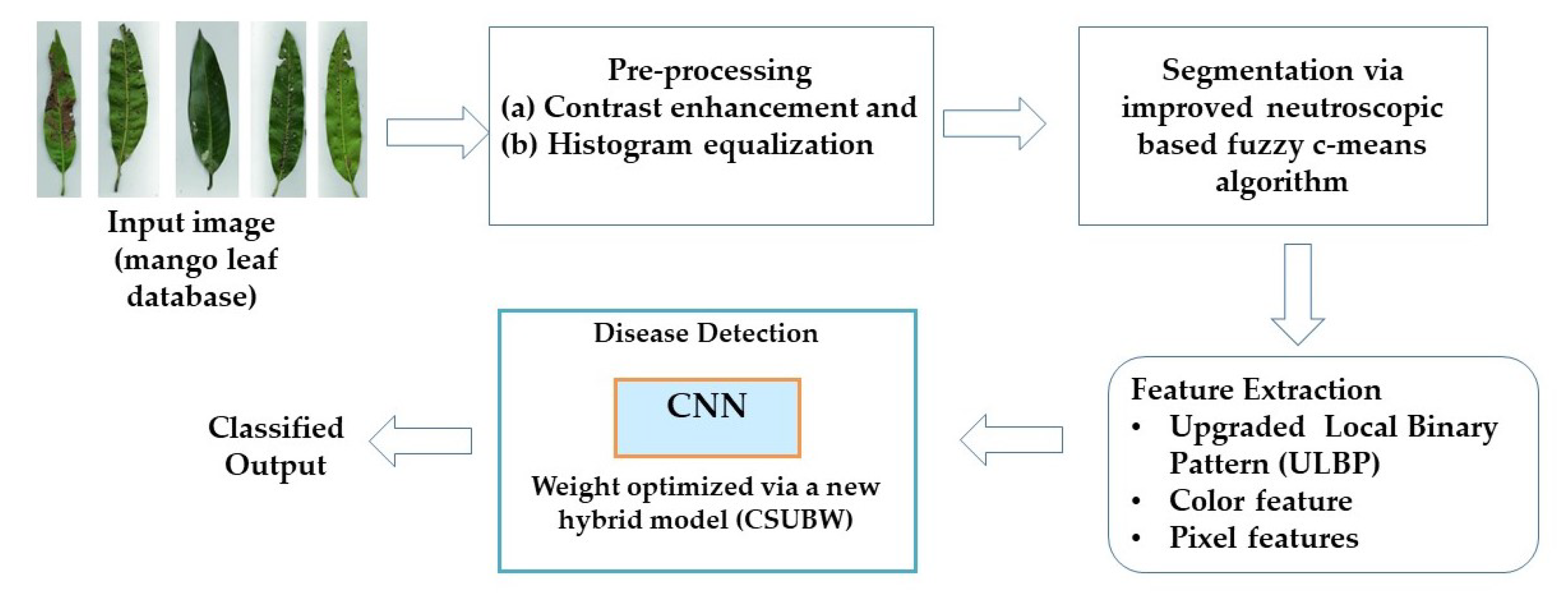
- Introduces a new geometric mean-based neutrosophic with fuzzy c-mean for segmenting the diseased region from the standard leaf regions;
- Extracts Upgraded Local Binary Pattern (ULBP) to train the detection model precisely, which results in the enhancement of texture features;
- Introduces a new optimized CNN model to detect the presence/absence of leaf disease in mango trees;
- Introduces a new hybrid meta-heuristic optimization model called Cat Swarm Updated Black Widow Model (CSUBW) to optimize the CNN.
2. Literature Review
3. Proposed Methodology
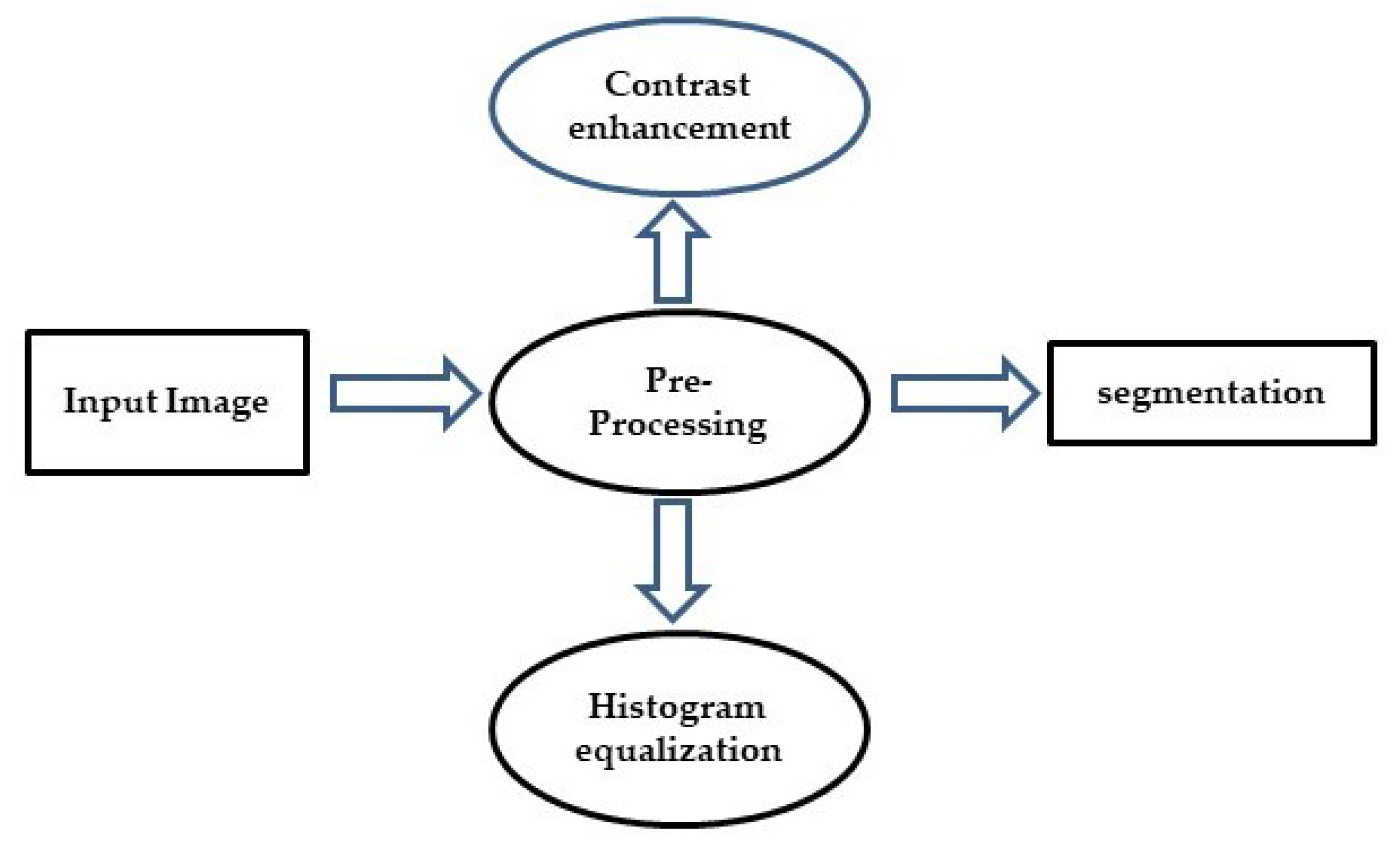
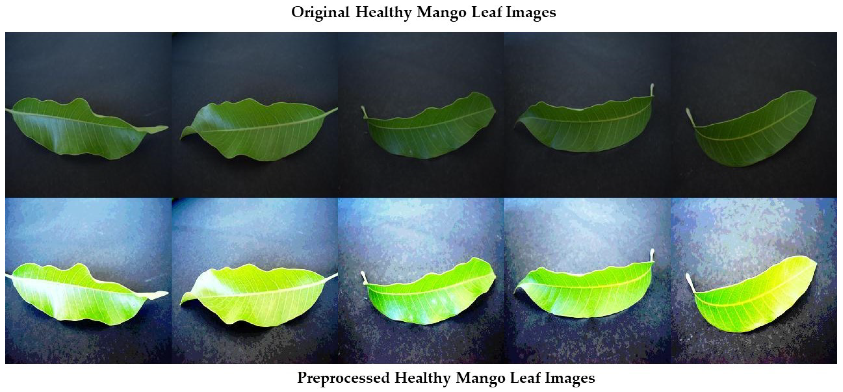
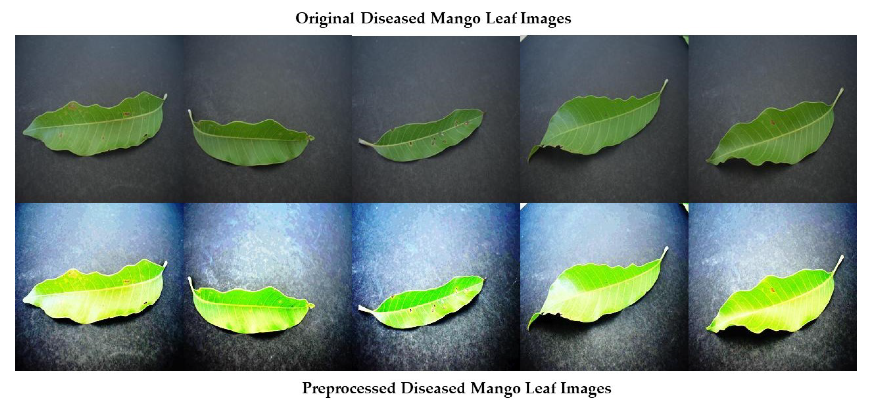
3.1. Preprocessing: Contrast Enhancement and Histogram Equialization
3.2. Contrast Enhancement
3.3. Histogram Equalization
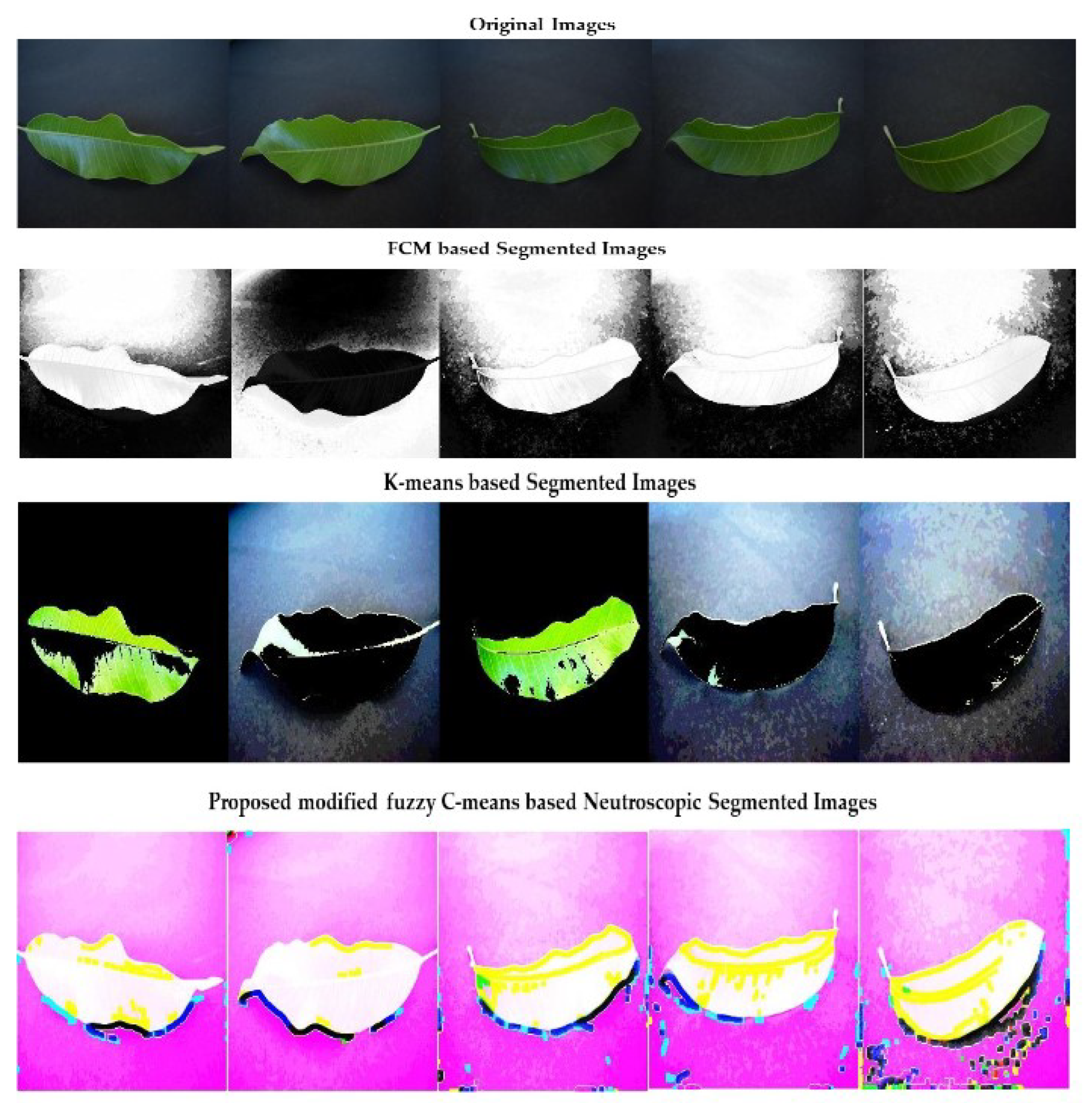
3.4. Proposed Image Segmentation Phase
Geometric Mean with Modified Fuzzy C-Means Based Neutrosophic Segmentation Phase
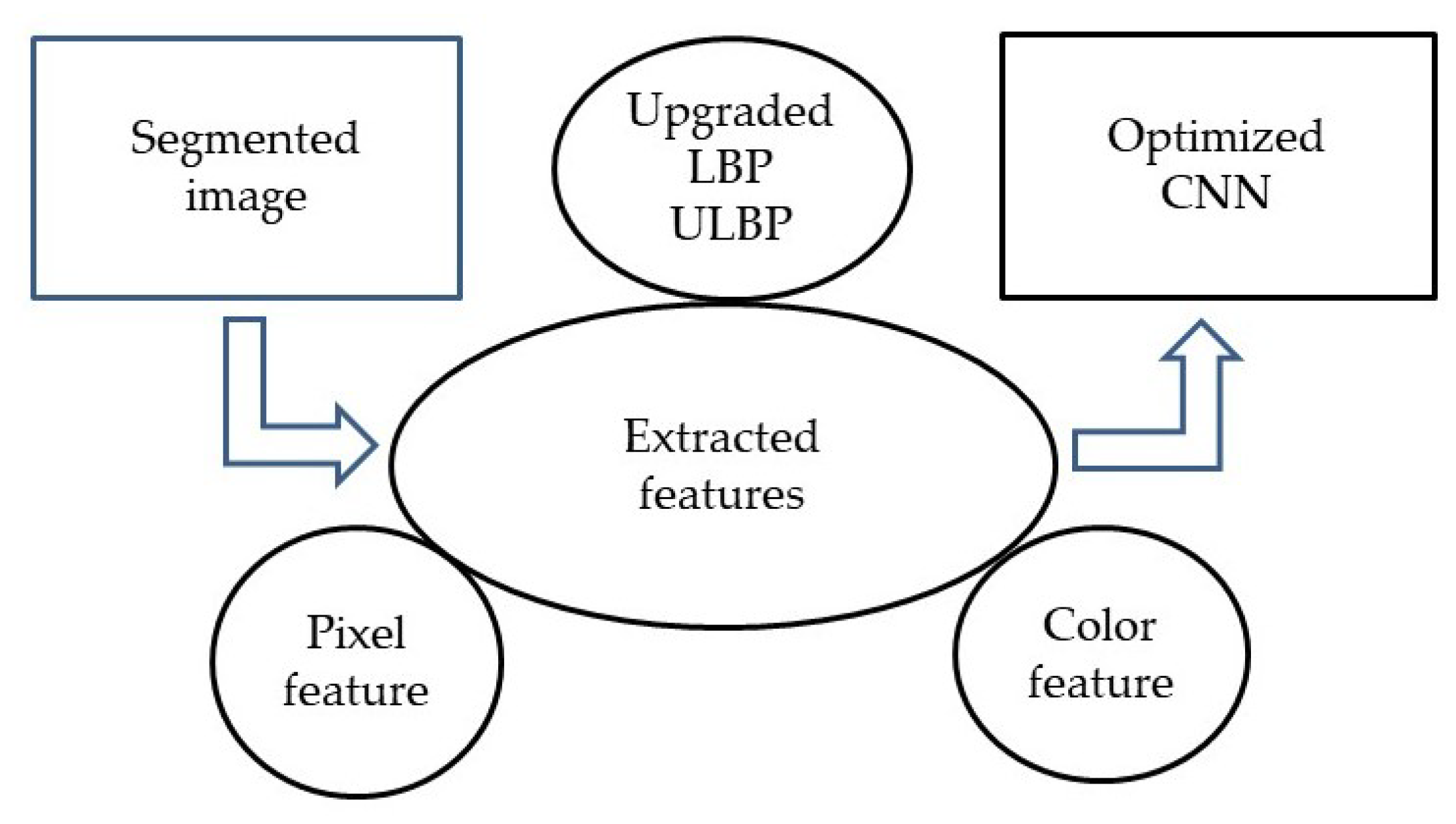
3.5. Proposed Feature Extraction Phase: Upgraded LBP, Color Feature and Pixel Feature
Upgraded LBP (ULBP)
3.6. Color and Pixel Features
4. Optimal Trained CNN for Disease Detection Model
4.1. Optimized CNN
4.2. CNN Training by Proposed CSUBW
- (a)
- Seeking Mode: for the present cat , J count of copies are made. Here, J is the SMP. If SPC value = true, then set J = (SMP-1) and set the present cat as the best one.
- (b)
- As per CDC, the SRD values are randomly plus or minus. Then, replace the old ones with the current ones.
- (c)
- For all the candidate points, the fitness function (Fit) is computed using Equation (27).
- (d)
- When all are not equivalent, the selecting probability is computed for every candidate point using Equation (28). When the fit is equivalent for every candidate point, the selecting probability is set as 1 for each candidate point.Here, the objective is minimization, so,
- (e)
- The point is randomly picked to move away from the candidate points, and the position of the cats is replaced.
- (a)
- For every dimension, the velocity of the search agent is updated using the newly proposed expression given in Equation (29).
- (b)
- Verify whether the velocity resides within the maximum velocity. In case the new velocity is beyond the range of the maximum velocity range, then set it to be equal to the limit.
- (c)
- Update the position of using the BWO’s mutation update model rather than using the traditional CSA update function. The mutation update model randomly selects the Mutepop number from the population (pop). Based on the mutation rate, the Mutepop is computed.
5. Results and Discussion
5.1. Simulation Setup
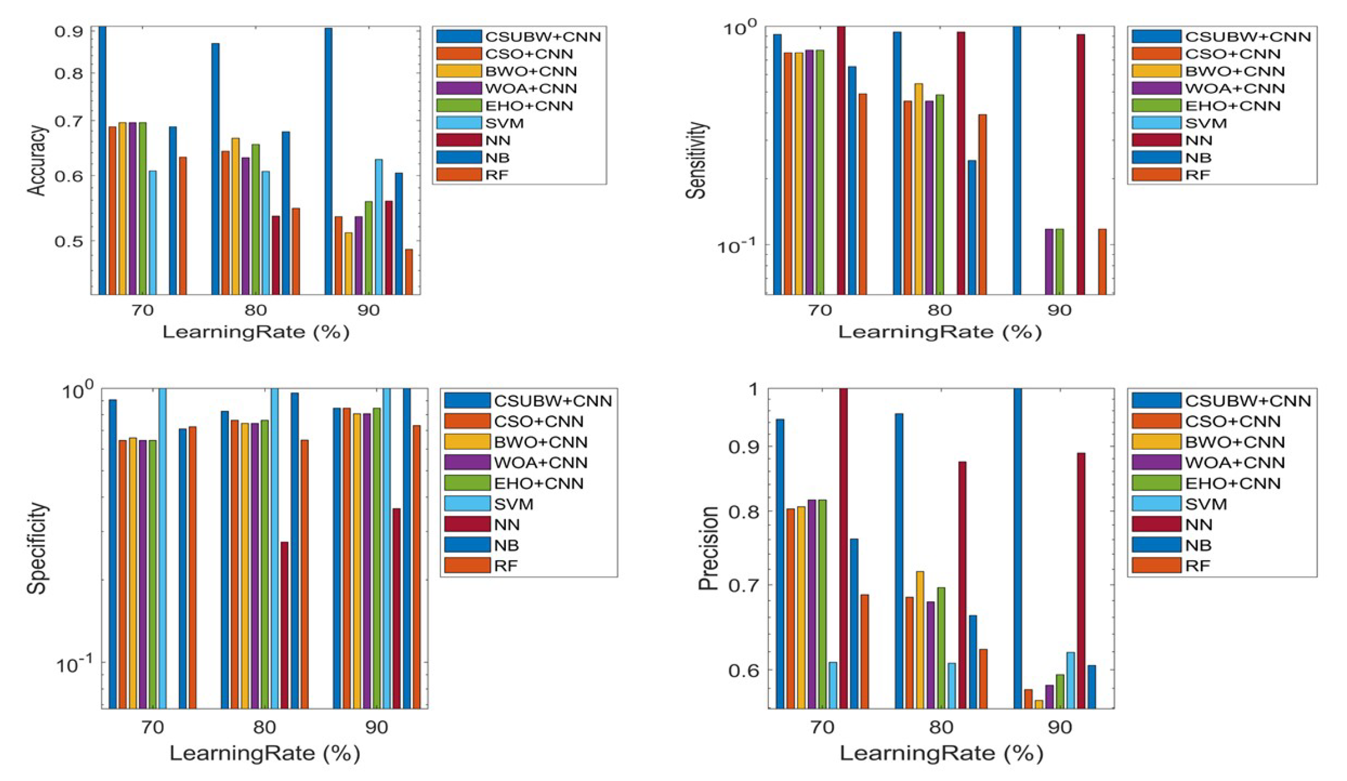
5.2. Performance Analysis
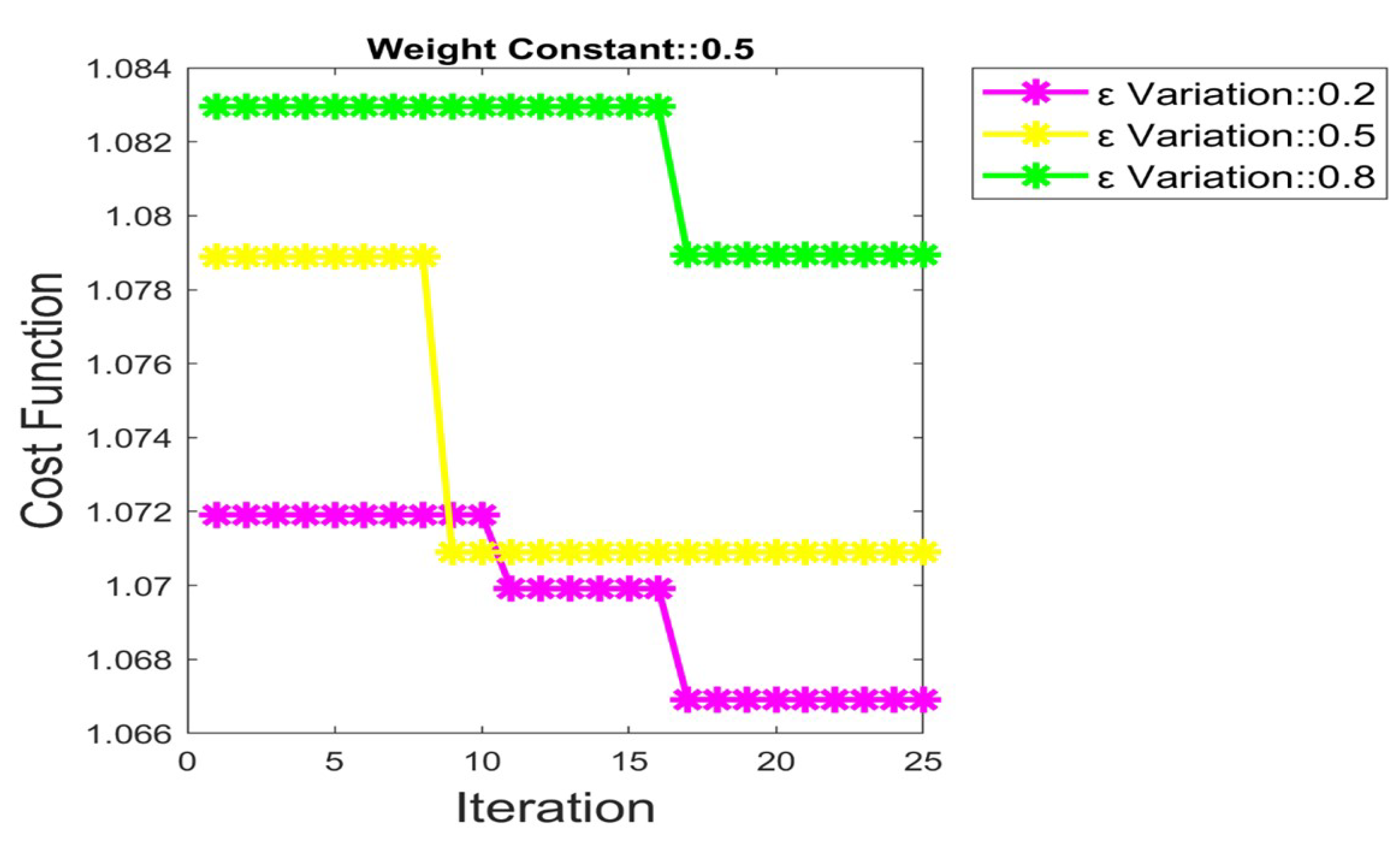
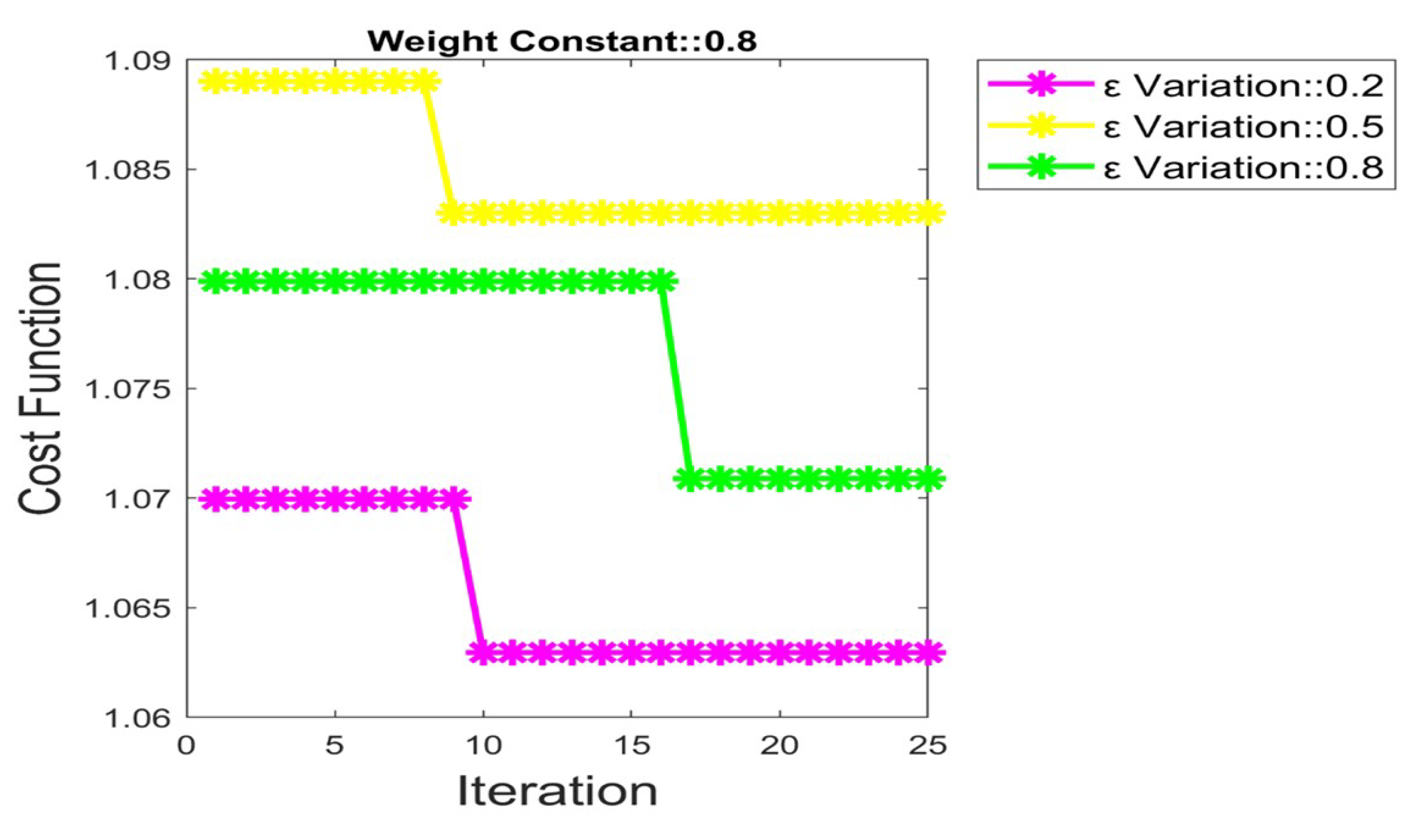
5.3. Convergence Analysis by Fixing = 0.2, 0.5 and 0.8
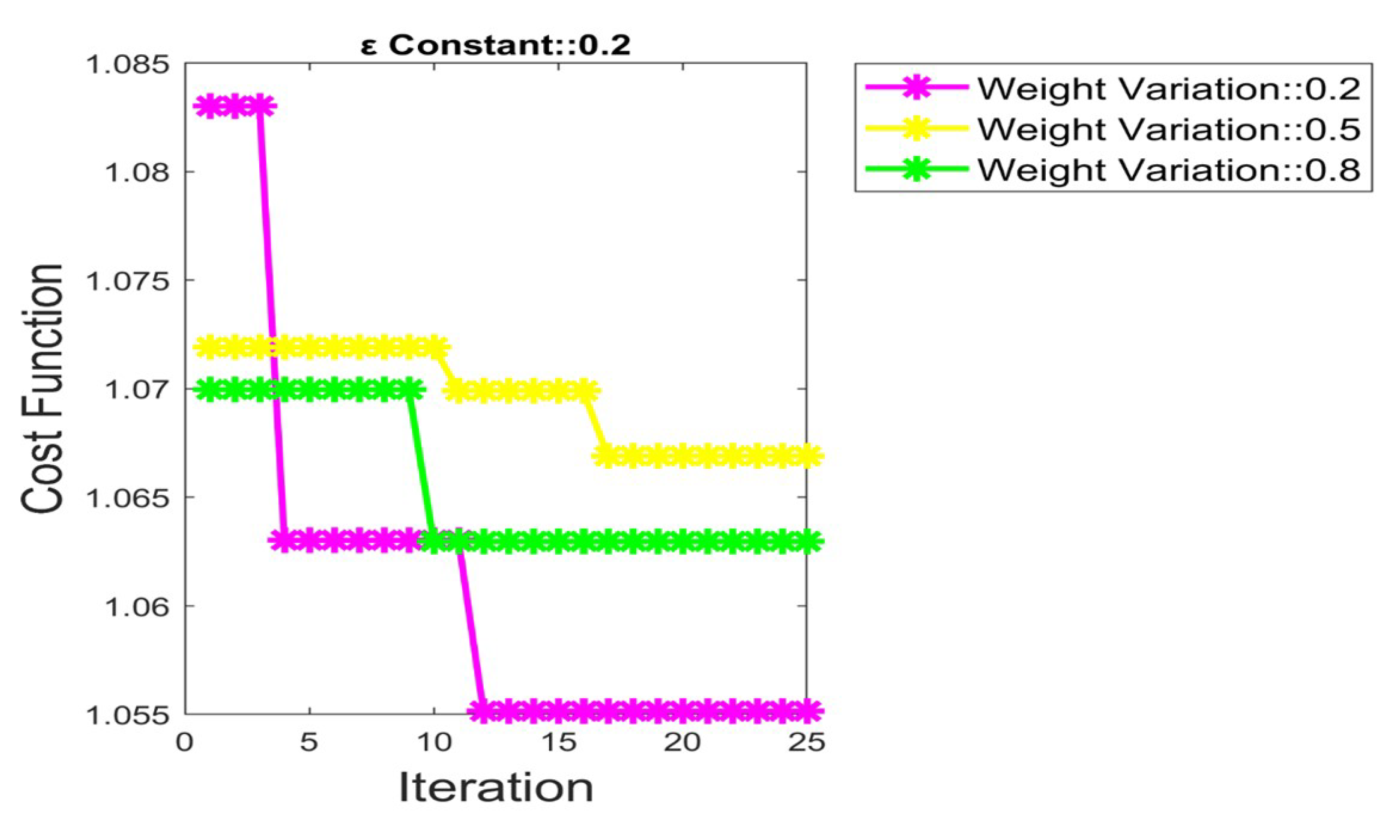
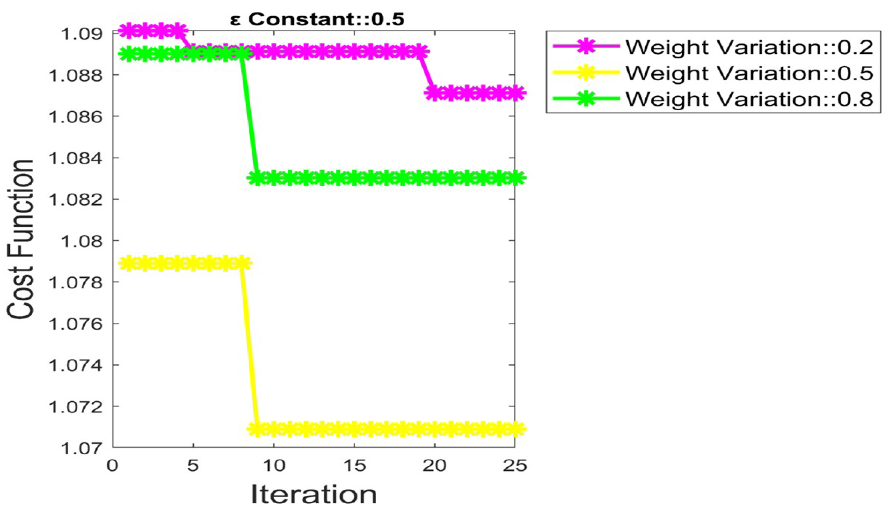
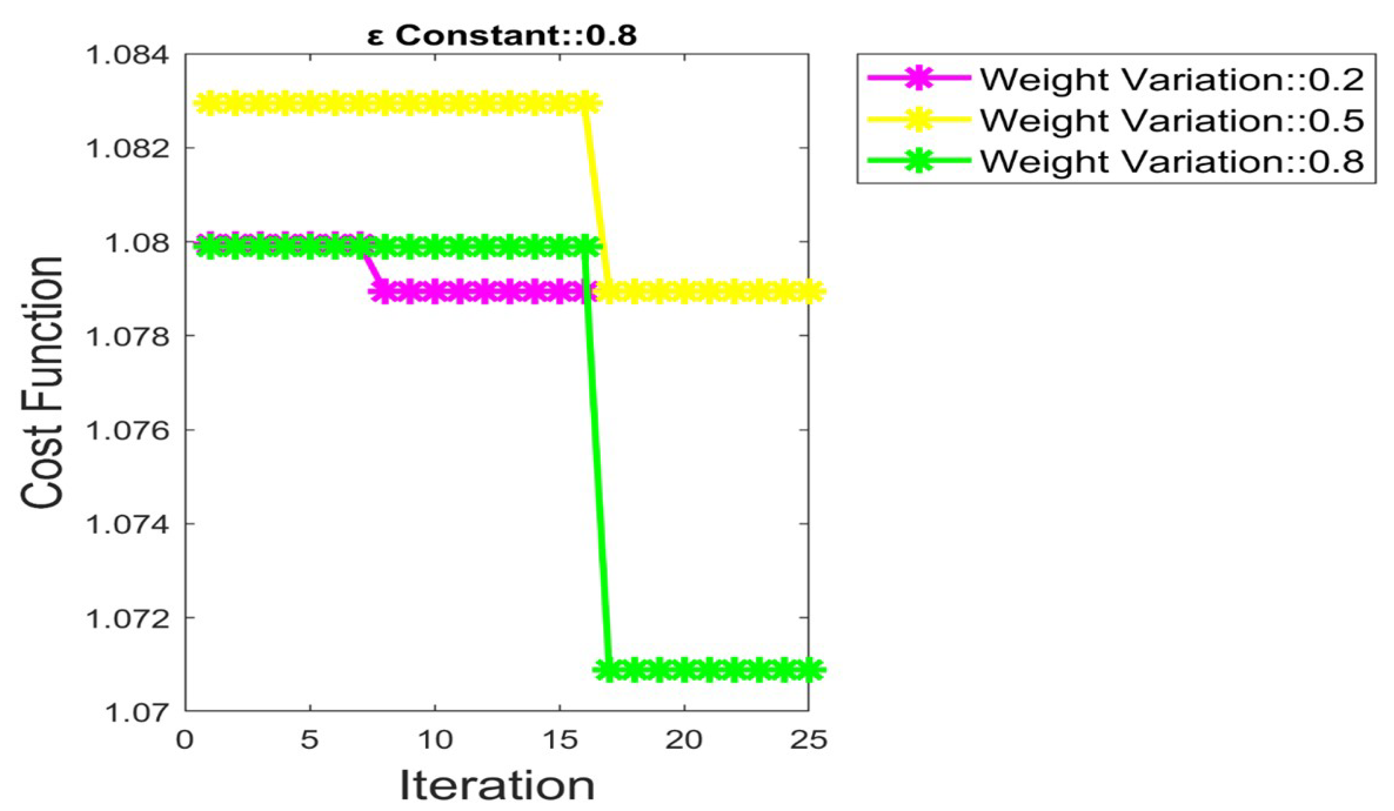
5.4. Convergence Analysis by Fixing = 0.2, 0.5 and 0.8
5.5. Overall Performance Analysis
6. Conclusions and Future Scope
Author Contributions
Funding
Institutional Review Board Statement
Informed Consent Statement
Data Availability Statement
Acknowledgments
Conflicts of Interest
References
- Chouhan, S.S.; Singh, U.P.; Jain, S. Web Facilitated Anthracnose Disease Segmentation from the Leaf of Mango Tree Using Radial Basis Function (RBF) Neural Network. Wirel. Pers. Commun. 2020, 113, 1279–1296. [Google Scholar] [CrossRef]
- Mia, M.; Roy, S.; Das, S.K.; Rahman, M. Mango leaf disease recognition using neural network and support vector machine. Iran. J. Comput. Sci. 2020, 3, 185–193. [Google Scholar] [CrossRef]
- Nagaraju, Y.; Sahana, T.S.; Swetha, S.; Hegde, S.U. Transfer Learning based Convolutional Neural Network Model for Classification of Mango Leaves Infected by Anthracnose. In Proceedings of the IEEE International Conference for Innovation in Technology (INOCON), Bangluru, India, 6–8 November 2020; pp. 1–7. [Google Scholar] [CrossRef]
- Sujatha, S.; Saravanan, N.; Sona, R. Disease identification in mango leaf using image processing. Adv. Nat. Appl. Sci. 2017, 11, 1–8. [Google Scholar]
- Singh, U.P.; Chouhan, S.S.; Jain, S.; Jain, S. Multilayer Convolution Neural Network for the Classification of Mango Leaves Infected by Anthracnose Disease. IEEE Access 2019, 7, 43721–43729. [Google Scholar] [CrossRef]
- Kabir, R.; Jahan, S.; Islam, M.R.; Rahman, N.; Islam, M.R. Discriminant Feature Extraction using Disease Segmentation for Automatic Leaf Disease Diagnosis. In Proceedings of the International Conference on Computing Advancements (ICCA 2020), Dhaka, Bangladesh, 10–12 January 2020. [Google Scholar]
- Liu, L.; Li, J.; Sun, Y. Research on the Plant Leaf Disease Region Extraction. In Proceedings of the International Conference on Video, Signal and Image Processing (VSIP 2019), Wuhan, China, 29–31 October 2019. [Google Scholar]
- Su, T.; Mu, S.; Dong, M.; Sun, W.; Shi, A. nAn Improved TrAdaBoost for Image Recognition of Unbalanced Plant Leaf Disease. In Proceedings of the 2019 8th International Conference on Computing and Pattern Recognition, Beijing, China, 23–25 October 2020. [Google Scholar]
- Trongtorkid, C.; Pramokchon, P. Expert system for diagnosis mango diseases using leaf symptoms analysis. In Proceedings of the 2018 International Conference on Digital Arts, Media and Technology (ICDAMT), Phayao, Thailand, 25–28 February 2018; pp. 59–64. [Google Scholar]
- Trang, K.; TonThat, L.; Thao, N.G.M.; Thi, N.T.T. Mango Diseases Identification by a Deep Residual Network with Contrast Enhancement and Transfer Learning. In Proceedings of the 2019 IEEE Conference on Sustainable Utilization and Development in Engineering and Technologies (CSUDET), Penang, Malaysia, 7–9 November 2019; pp. 138–142. [Google Scholar] [CrossRef]
- Tumang, G.S. Pests and Diseases Identification in Mango using MATLAB. In Proceedings of the 2019 5th International Conference on Engineering, Applied Sciences and Technology (ICEAST), Luang Prabang, Laos, 2–5 July 2019; pp. 1–4. [Google Scholar] [CrossRef]
- Madiwalar, S.C.; Wyawahare, M.V. Plant disease identification: A comparative study. In Proceedings of the 2017 International Conference on Data Management, Analytics and Innovation (ICDMAI), Pune, India, 24–26 February 2017; pp. 13–18. [Google Scholar] [CrossRef]
- Arya, S.; Singh, R. A Comparative Study of CNN and AlexNet for Detection of Disease in Potato and Mango leaf. In Proceedings of the 2019 International Conference on Issues and Challenges in Intelligent Computing Techniques (ICICT), Ghaziabad, India, 27–28 September 2019; pp. 1–6. [Google Scholar] [CrossRef]
- Setyanto, A.; Agastya, I.M.A.; Priantoro, H.; Chandramouli, K. User Evaluation of Mobile based Smart Mango Pest Identification. In Proceedings of the 2020 8th International Conference on Cyber and IT Service Management (CITSM), Pangkal, Indonesia, 23–24 October 2020; pp. 1–7. [Google Scholar] [CrossRef]
- Swetha, K.; Venkataraman, V.; Sadhana, G.D.; Priyatharshini, R. Hybrid approach for anthracnose detection using intensity and size features. In Proceedings of the 2016 IEEE Technological Innovations in ICT for Agriculture and Rural Development (TIAR), Chennai, India, 15–16 July 2016; pp. 28–32. [Google Scholar] [CrossRef]
- Pham, T.N.; Van Tran, L.; Dao, S.V.T. Early Disease Classification of Mango Leaves Using Feed-Forward Neural Network and Hybrid Metaheuristic Feature Selection. IEEE Access 2020, 8, 189960–189973. [Google Scholar] [CrossRef]
- Nishat, M.M.; Faisal, F. An Investigation of Spectroscopic Characterization on Biological Tissue. In Proceedings of the 2018 4th International Conference on Electrical Engineering and Information & Communication Technology (iCEEiCT), Dhaka, Bangladesh, 13–15 September 2018; pp. 290–295. [Google Scholar] [CrossRef]
- Yamparala, R.; Challa, R.; Kantharao, V.; Krishna, P.S.R. Computerized Classification of Fruits using Convolution Neural Network. In Proceedings of the 2020 7th International Conference on Smart Structures and Systems (ICSSS), Chennai, India, 23–24 July 2020; pp. 1–4. [Google Scholar] [CrossRef]
- Ullagaddi, S.B.; Raju, S.V. Disease recognition in Mango crop using modified rotational kernel transform features. In Proceedings of the 2017 4th International Conference on Advanced Computing and Communication Systems (ICACCS), Coimbatore, India, 6–7 January 2017; pp. 1–8. [Google Scholar] [CrossRef]
- Kumar, P.; Ashtekar, S.; Jayakrishna, S.S.; Bharath, K.P.; Vanathi, P.T.; Kumar, M.R. Classification of Mango Leaves Infected by Fungal Disease Anthracnose Using Deep Learning. In Proceedings of the International Conference on Computing Methodologies and Communication (ICCMC), Erode, India, 8–10 April 2021. [Google Scholar] [CrossRef]
- Kaur, S. Contrast Enhancement Techniques for Images—A Visual Analysis. Int. J. Comput. Appl. 2013, 64, 20–25. [Google Scholar]
- Histogram Equalization. Available online: https://towardsdatascience.com/histogram-equalization-5d1013626e64 (accessed on 4 August 2021).
- Sairamya, N.J.; Susmitha, L.; George, S.T.; Subathra, M.S.P. Hybrid approach for classification of electroencephalographic signals using time–frequency images with wavelets and texture features. In Intelligent Data Analysis for Biomedical Applications; Academic Press: Cambridge, MA, USA, 2019; Chapter 12. [Google Scholar]
- Pixel Feature. Available online: https://www.tutorialspoint.com/dip/brightness_and_contrast.htm (accessed on 4 August 2021).
- Chandanapalli, S.B.; Reddy, E.S.; Lakshmi, D.R. Convolutional Neural Network for Water Quality Prediction in WSN. J. Netw. Commun. Syst. 2019, 2, 40–47. [Google Scholar]
- Gangappa, M.; Mai, C.; Sammulal, P. Enhanced Crow Search Optimization Algorithm and Hybrid NN-CNN Classifiers for Classification of Land Cover Images. Multimed. Res. 2019, 2, 12–22. [Google Scholar]
- Darekar, R.V.; Dhande, A.P. Emotion Recognition from Speech Signals Using DCNN with Hybrid GA-GWO Algorithm. Multimed. Res. 2019, 2, 12–22. [Google Scholar]
- Beno, M.M.; Valarmathi, I.R.; Swamy, S.M.; Rajakumar, B.R. Threshold prediction for segmenting tumour from brain MRI scans. Int. J. Imaging Syst. Technol. 2014, 24, 129–137. [Google Scholar] [CrossRef]
- Wagh, M.B.; Gomathi, N. Improved GWO-CS Algorithm-Based Optimal Routing Strategy in VANET. J. Netw. Commun. Syst. 2019, 2, 34–42. [Google Scholar]
- Srinivas, V.; Santhirani, C. Hybrid Particle Swarm Optimization-Deep Neural Network Model for Speaker Recognition. Multimed. Res. 2020, 3, 1–10. [Google Scholar]
- Netaji, V.K.; Bhole, G.P. Optimal Container Resource Allocation Using Hybrid SA-MFO Algorithm in Cloud Architecture. Multimed. Res. 2020, 3, 11–20. [Google Scholar]
- Ashok Kumar, C.; Vimala, R. Load Balancing in Cloud Environment Exploiting Hybridization of Chicken Swarm and Enhanced Raven Roosting Optimization Algorithm. Multimed. Res. 2020, 3, 45–55. [Google Scholar]
- Roy, M.R.G. Economic dispatch problem in power system using hybrid Particle Swarm optimization and enhanced Bat optimization algorithm. J. Comput. Mech. Power Syst. Control 2020, 3, 27–33. [Google Scholar]
- Al Raisi, A.A.J. Hybird Particle Swarm Optimization and Gravitational Search Algorithm for economic dispatch in power system. J. Comput. Mech. Power Syst. Control 2020, 3, 34–40. [Google Scholar] [CrossRef]
- Chu, S.C.; Tsai, P.W.; Pan, J.S. Cat Swarm Optimization. In Proceedings of the 9th Pacific Rim International Conference on Artificial Intelligence, Guilin, China, 7–11 August 2006; pp. 854–858. [Google Scholar]
- Hayyolalam, V.; Kazem, A.A.P. Black Widow Optimization Algorithm: A novel met. a-heuristic approach for solving engineering optimization problems. Eng. Appl. Artif. Intell. 2020, 87, 103249. [Google Scholar] [CrossRef]
- Available online: https://www.kaggle.com/agbajeabdullateef/a-database-of-leaf-images-from-mendeley-data (accessed on 1 August 2021).


| Author | Adopted Methodology | Advantages | Drawbacks |
|---|---|---|---|
| Chouhan et al. [1] | Radial Basis Function (RBF) Neural Network | higher specificity and sensitivity, intuitive, user-friendly | need to overcome over-segmentation problem; highly prone to noise; not applicable in industrial applications |
| Mia et al. [2] | neural network | consumes less time | accuracy of classification is lower; risk of over-fitting; not used in industrial applications |
| Venkatesh et al. [3] | VGGNet model | simple and cost-effective; used in industrial applications | lower detection accuracy |
| Pham et al. [16] | Feed-Forward Neural Network and Hybrid Metaheuristic Feature Selection | higher testing accuracy, recall, precision and F1-score | higher computational complexity in terms of time and cost |
| Singh et al. [13] | Multilayer Convolution Neural Network | higher classification accuracy (97.13%) computationally efficient; used in different industrial conditions | highly prone to noise |
| Ullagaddi and Raju [19] | Modified Rotational Kernel Transform Features | higher reorganising accuracy and segmentation accuracy | lower miss rate, specificity and sensitivity; not applicable in industrial conditions |
| Kumar et al. [20] | CNN | higher classification accuracy; used in different industrial constraints | lower sensitivity and specificity higher misclassification |
| Sujatha et al. [4] | ANN | less prone to noise, efficient extraction metod92.31 | higher computational complexity; not applicable in industrial conditions |
Publisher’s Note: MDPI stays neutral with regard to jurisdictional claims in published maps and institutional affiliations. |
© 2022 by the authors. Licensee MDPI, Basel, Switzerland. This article is an open access article distributed under the terms and conditions of the Creative Commons Attribution (CC BY) license (https://creativecommons.org/licenses/by/4.0/).
Share and Cite
Mohapatra, M.; Parida, A.K.; Mallick, P.K.; Zymbler, M.; Kumar, S. Botanical Leaf Disease Detection and Classification Using Convolutional Neural Network: A Hybrid Metaheuristic Enabled Approach. Computers 2022, 11, 82. https://0-doi-org.brum.beds.ac.uk/10.3390/computers11050082
Mohapatra M, Parida AK, Mallick PK, Zymbler M, Kumar S. Botanical Leaf Disease Detection and Classification Using Convolutional Neural Network: A Hybrid Metaheuristic Enabled Approach. Computers. 2022; 11(5):82. https://0-doi-org.brum.beds.ac.uk/10.3390/computers11050082
Chicago/Turabian StyleMohapatra, Madhumini, Ami Kumar Parida, Pradeep Kumar Mallick, Mikhail Zymbler, and Sachin Kumar. 2022. "Botanical Leaf Disease Detection and Classification Using Convolutional Neural Network: A Hybrid Metaheuristic Enabled Approach" Computers 11, no. 5: 82. https://0-doi-org.brum.beds.ac.uk/10.3390/computers11050082