
Energy-Efficient Deterministic Approach for Coverage Hole Detection in Wireless Underground Sensor Network: Mathematical Model and Simulation


Abstract
:1. Introduction
- 1
- A polynomial-time algorithm is proposed which can effectively detect all the holes presented in the network. Most of the existing solutions are centralized and work for hybrid networks. Such solutions are not scalable and therefore not suitable for WUSNs. WUSNs consist of static nodes and require solutions that possess low complexity and are scalable. Our algorithm is very well suited for WUSNSs.
- 2
- Our algorithm requires only the location/coordinate information of the nodes.
- 3
- Our algorithm is energy-efficient. The proposed coverage hole detection algorithm was run for the network lifetime, where all nodes communicate using the LEACH protocol. The algorithm avoids unnecessary computation and extra communication overheads which reduce the network lifetime. The residual energy after every round was noted. Based on the residual energy in the network, a new node deployment can be pre-planned. Considering the energy factor provides a comprehensive and wide-ranging viewpoint. The algorithm performs efficiently during the complete lifetime of the network. Extensive simulations were conducted to validate the performance of our proposed algorithm. The algorithm was tested by varying the number and sensing radius of the nodes. It works very well in spite of the nodes’ distribution and density. The algorithm has a short run time with the lowest cost and provides an accurate solution. The results show that the method is reliable, cost-effective, and energy-efficient.
2. Related Work
- ─
- Uniform and dense deployment of sensor nodes with a statistical distribution is required in range-based techniques which is not always feasible.
- ─
- In connectivity-based techniques, topology/connectivity information between nodes is needed which adds an extra communication overhead in the network and thus reduces the lifetime of the network. This will increase the deployment frequency of underground nodes and increase the cost and complexity.
- ─
- In many techniques, sensor networks are hybrid, i.e., a network containing both static and mobile nodes. However, in WUSNs, all the sensor nodes are static, so the algorithm needs to be designed with this factor taken into consideration.
3. Mathematical Model and Methodology
3.1. Assumptions
- 1
- Each node knows its location.
- 2
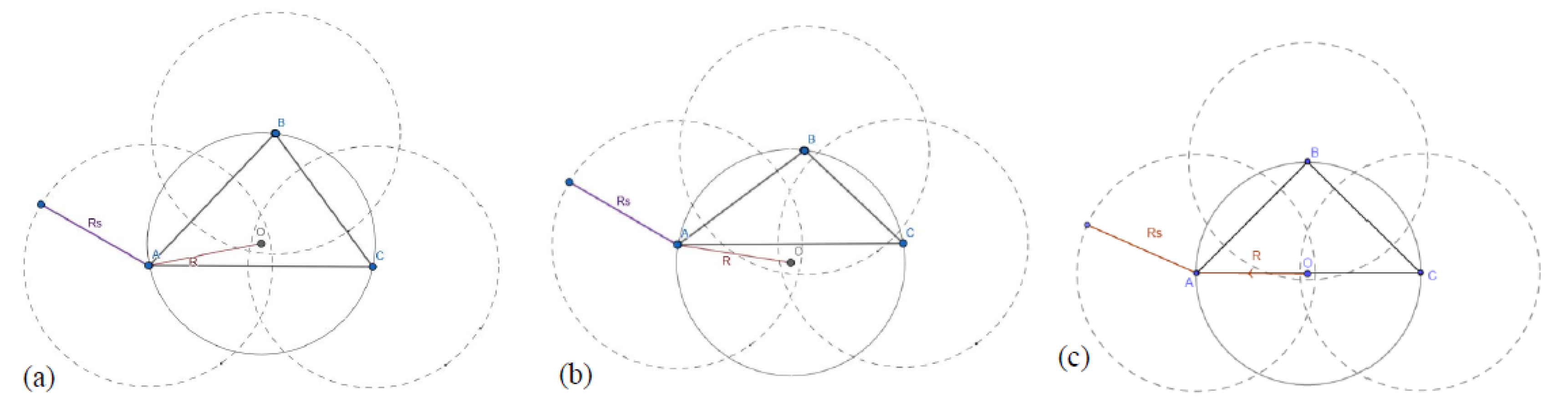
- The communication radius (Rc) is larger than or equal to two times the sensing radius (Rs).
- 3
- The sensing area of every sensor node is a circular disc with a sensing radius of Rs.
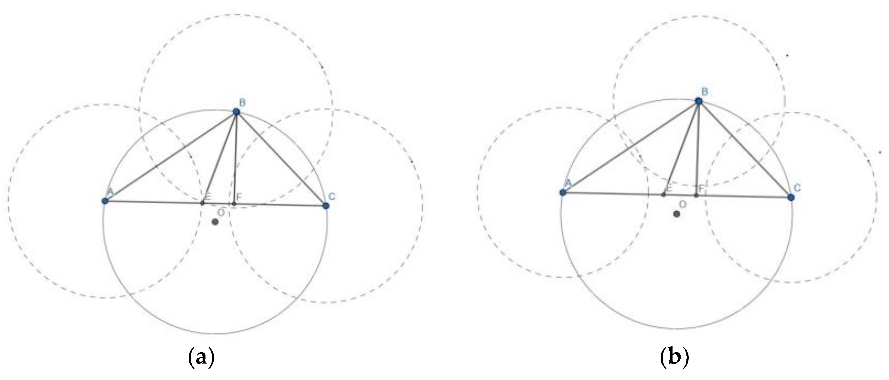
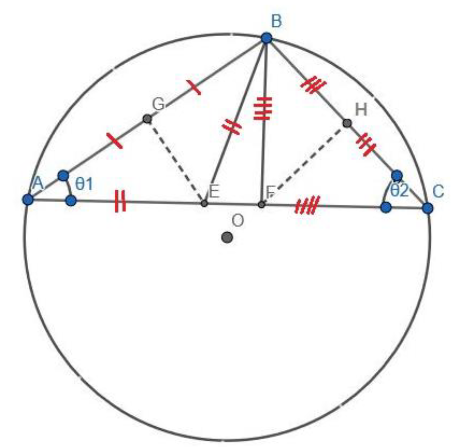
3.2. Mathematical Formulations
4. Coverage Hole Detection Algorithm
| Algorithm 1: Coverage Hole Detection for WUSNs. |
Input:
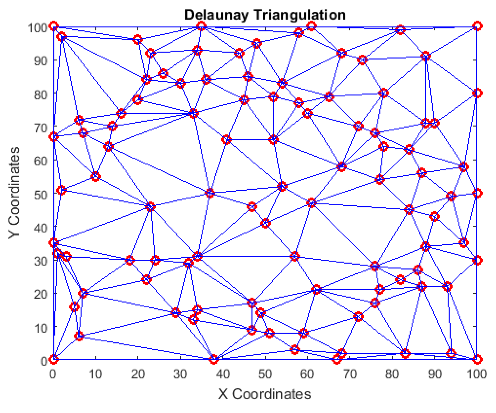
Marking of Holes in Delaunay triangles H = [H1, H2,…Hm], if Hi is NULL, then there is no Hole else There is a Hole and Hi contains coordinates of the circumcenter of DTi. |
| Algorithm 2: Estimation of Coverage Holes in the Lifetime of a WUSN. |
Input:
|
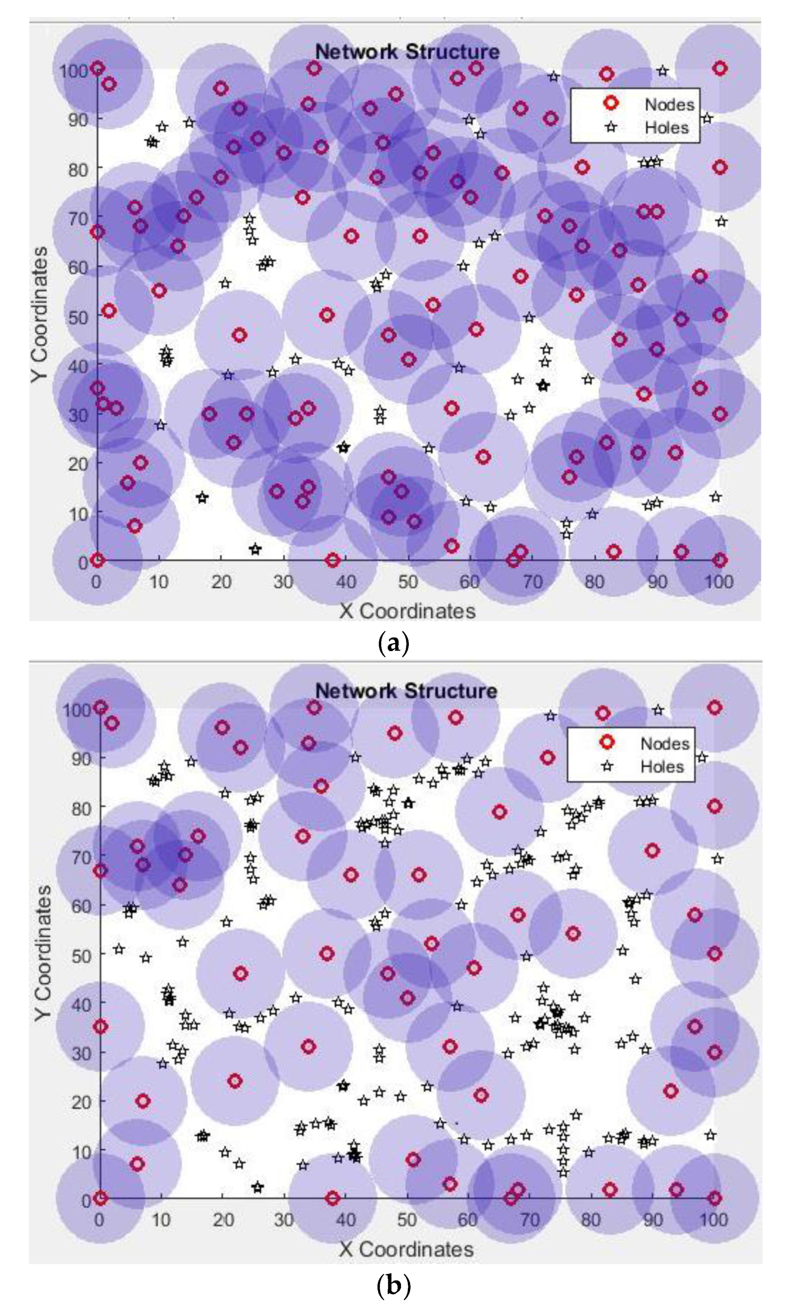
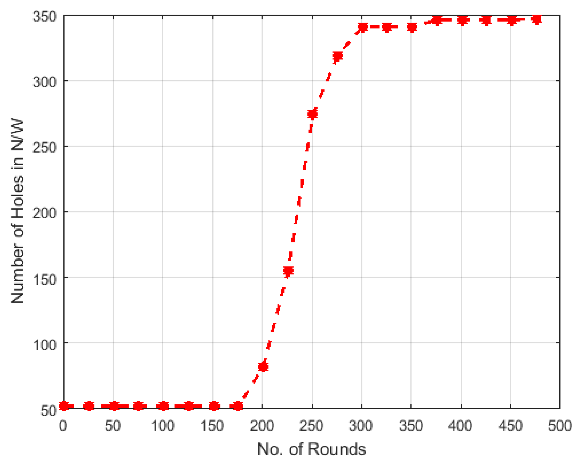
5. Simulation Results
6. Discussion
7. Conclusions
Author Contributions
Funding
Data Availability Statement
Acknowledgments
Conflicts of Interest
References
- Silva, A.R.; Vuran, M.C. Communication with Aboveground Devices in Wireless Underground Sensor Networks: An Empirical Study. In Proceedings of the 2010 IEEE international conference on communications, Cape Town, South Africa, 23–27 May 2010; pp. 1–6. [Google Scholar]
- Vuran, M.C.; Silva, A.R. Communication through Soil in Wireless Underground Sensor Networks–Theory and Practice. In Sensor Networks; Springer: New York City, NY, USA, 2010; pp. 309–347. [Google Scholar]
- Akyildiz, I.F.; Stuntebeck, E.P. Wireless Underground Sensor Networks: Research Challenges. Ad Hoc Netw. 2006, 4, 669–686. [Google Scholar] [CrossRef]
- Yoon, S.-U.; Cheng, L.; Ghazanfari, E.; Pamukcu, S.; Suleiman, M.T. A radio propagation model for wireless underground sensor networks. In Proceedings of the 2011 IEEE Global Telecommunications Conference-GLOBECOM 2011, Houston, TX, USA, 5–9 December 2011; pp. 1–5. [Google Scholar]
- Alibakhshikenari, M.; Virdee, B.S.; Althuwayb, A.A.; Aïssa, S.; See, C.H.; Abd-Alhameed, R.A.; Falcone, F.; Limiti, E. Study on on-chip antenna design based on metamaterial-inspired and substrate-integrated waveguide properties for millimetre-wave and THz integrated-circuit applications. J. Infrared Millim. Terahertz Waves 2021, 42, 17–28. [Google Scholar] [CrossRef]
- Shirkolaei, M.M. Wideband linear microstrip array antenna with high efficiency and low side lobe level. Int. J. RF Microw. Comput. Aided Eng. 2020, 30, e22412. [Google Scholar] [CrossRef]
- Lin, K.; Hao, T. Experimental link quality analysis for LoRa-based wireless underground sensor networks. IEEE Internet Things J. 2020, 8, 6565–6577. [Google Scholar] [CrossRef]
- Silva, B.; Fisher, R.M.; Kumar, A.; Hancke, G.P. Experimental link quality characterization of wireless sensor networks for underground monitoring. IEEE Trans. Ind. Inform. 2015, 11, 1099–1110. [Google Scholar] [CrossRef] [Green Version]
- Kaushik, A. Multiple Hole Detection in Wireless Underground Sensor Networks. In Proceedings of the Communication and Computing Systems: Proceedings of the 2nd International Conference on Communication and Computing Systems ICCCS 2018, Gurgaon, India, 1–2 December 2018; p. 157. [Google Scholar]
- Bi, K.; Gu, N.; Tu, K.; Dong, W. Neighborhood-Based Distributed Topological Hole Detection Algorithm in Sensor Networks. In Proceedings of the IET International Conference on Wireless, Mobile and Multimedia Networks, Hangzhou, China, 6–9 November 2006; pp. 1–4. [Google Scholar]
- Ghosh, A.; Das, S.K. Coverage and Connectivity Issues in Wireless Sensor Networks: A Survey. Pervasive Mob. Comput. 2008, 4, 303–334. [Google Scholar] [CrossRef]
- Nguyen, P.L.; Ji, Y.; Liu, Z.; Vu, H.; Nguyen, K.-V. Distributed Hole-Bypassing Protocol in WSNs with Constant Stretch and Load Balancing. Comput. Netw. 2017, 129, 232–250. [Google Scholar] [CrossRef]
- Antil, P.; Malik, A. Hole Detection for Quantifying Connectivity in Wireless Sensor Networks: A Survey. J. Comput. Netw. Commun. 2014, 2014, 969501. [Google Scholar] [CrossRef] [Green Version]
- Watfa, M.K.; Commuri, S. Energy-Efficient Approaches to Coverage Holes Detection in Wireless Sensor Networks. In Proceedings of the 2006 IEEE Conference on Computer Aided Control System Design, 2006 IEEE International Conference on Control Applications, 2006 IEEE International Symposium on Intelligent Control, Munich, Germany, 4–6 October 2006; pp. 131–136. [Google Scholar]
- De Silva, V.; Ghrist, R.; Muhammad, A. Blind Swarms for Coverage in 2-D. In Proceedings of the 1st Conference on Robotics: Science and Systems, Massachusetts Institute of Technology, Cambridge, MA, USA; pp. 335–342. Available online: http://math.uchicago.edu/~shmuel/AAT-readings/Sensory%20networks/blind%20swarms.pdf (accessed on 1 April 2022).
- De Silva, V.; Ghrist, R. Coordinate-Free Coverage in Sensor Networks with Controlled Boundaries via Homology. Int. J. Robot. Res. 2006, 25, 1205–1222. [Google Scholar] [CrossRef]
- Yao, J.; Zhang, G.; Kanno, J.; Selmic, R. Decentralized Detection and Patching of Coverage Holes in Wireless Sensor Networks. In Intelligent Sensing, Situation Management, Impact Assessment, and Cyber-Sensing; International Society for Optics and Photonics: Orlando, FL, USA, 2009; Volume 7352, p. 73520V. [Google Scholar]
- Ghosh, P.; Gao, J.; Gasparri, A.; Krishnamachari, B. Distributed Hole Detection Algorithms for Wireless Sensor Networks. In Proceedings of the 2014 IEEE 11th International Conference on Mobile Ad Hoc and Sensor Systems, Philadelphia, PA, USA, 28–30 October 2014; pp. 257–261. [Google Scholar]
- Yan, F.; Martins, P.; Decreusefond, L. Connectivity-Based Distributed Coverage Hole Detection in Wireless Sensor Networks. In Proceedings of the 2011 IEEE Global Telecommunications Conference GLOBECOM 2011, Houston, TX, USA, 5–9 December 2011; pp. 1–6. [Google Scholar]
- Khan, I.M.; Jabeur, N.; Zeadally, S. Hop-Based Approach for Holes and Boundary Detection in Wireless Sensor Networks. IET Wirel. Sens. Syst. 2012, 2, 328–337. [Google Scholar] [CrossRef]
- Wang, G.; Cao, G.; La Porta, T.F. Movement-Assisted Sensor Deployment. IEEE Trans. Mob. Comput. 2006, 5, 640–652. [Google Scholar] [CrossRef]
- Zhang, C.; Zhang, Y.; Fang, Y. Localized Algorithms for Coverage Boundary Detection in Wireless Sensor Networks. Wirel. Netw. 2009, 15, 3–20. [Google Scholar] [CrossRef]
- Hatcher, A. Algebraic Topology; Tsinghua University Press Co., Ltd: Beijing, China, 2005. [Google Scholar]
- Bejerano, Y. Coverage Verification without Location Information. IEEE Trans. Mob. Comput. 2011, 11, 631–643. [Google Scholar] [CrossRef]
- Funke, S.; Klein, C. Hole Detection or: How Much Geometry Hides in Connectivity? In Proceedings of the Twenty-Second Annual Symposium on Computational Geometry, Sedona, AZ, USA, 5–7 June 2006; pp. 377–385. [Google Scholar]
- Li, X.; Hunter, D.K. Distributed Coordinate-Free Hole Recovery. In Proceedings of the ICC Workshops-2008 IEEE International Conference on Communications Workshops, Beijing, China, 19–23 May 2008; pp. 189–194. [Google Scholar]
- Bi, K.; Tu, K.; Gu, N.; Dong, W.L.; Liu, X. Topological Hole Detection in Sensor Networks with Cooperative Neighbors. In Proceedings of the 2006 International Conference on Systems and Networks Communications ICSNC’06, Tahiti, French Polynesia, 29 October–3 November 2006; p. 31. [Google Scholar]
- Ghrist, R.; Muhammad, A. Coverage and Hole-Detection in Sensor Networks via Homology. In Proceedings of the IPSN 2005 Fourth International Symposium on Information Processing in Sensor Networks, Los Angeles, CA, USA, 24–27 April 2005; pp. 254–260. [Google Scholar]
- Corke, P.; Peterson, R.; Rus, D. Finding Holes in Sensor Networks. In Proceedings of the 2007 IEEE International Conference on Robotics and Automation, Roma, Italy, 10–14 April 2007; Available online: https://www.researchgate.net/profile/Daniela_Rus/publication/268256993_Finding_Holes_in_Sensor_Networks/links/56d0439f08ae059e375cfbae.pdf (accessed on 1 April 2022).
- Yangy, S.; Liz, M.; Wu, J. Scan-Based Movement-Assisted Sensor Deployment Methods in Wireless Sensor Networks. IEEE Trans. Parallel Distrib. Syst. 2007, 18, 1108–1121. [Google Scholar] [CrossRef]
- Shirsat, A.; Bhargava, B. Local Geometric Algorithm for Hole Boundary Detection in Sensor Networks. Secur. Commun. Netw. 2011, 4, 1003–1012. [Google Scholar] [CrossRef]
- Senouci, M.R.; Mellouk, A.; Assnoune, K. Localized Movement-Assisted Sensor Deployment Algorithm for Hole Detection and Healing. IEEE Trans. Parallel Distrib. Syst. 2013, 25, 1267–1277. [Google Scholar] [CrossRef]
- Aurenhammer, F.; Klein, R.; Lee, D.-T. Voronoi Diagrams and Delaunay Triangulations; World Scientific Publishing Company: Singapore, 2013. [Google Scholar]
- Rakovic, S.; Grieder, P.; Jones, C. Computation of Voronoi Diagrams and Delaunay Triangulation via Parametric Linear Programming; ETH (Eidgenössische Technische Hochschule): Zurich, Switzerland, 2004. [Google Scholar]
- Low-Energy Adaptive Clustering Hierarchy; In Wikipedia, The Free Encyclopedia; Page Version ID: 1076138763. 2019. Available online: https://en.wikipedia.org/wiki/Low-energy_adaptive_clustering_hierarchy (accessed on 1 April 2022).


| Type of Technique | Paper | Model/Concept Used | Limitations/Constraints |
|---|---|---|---|
| Range-Based Techniques | [15] | Blind swarm-based algorithm | Centralized computation. Minimum node requirement for optimal coverage. |
| [24] | Two-anchor (TA) and cyclic segment sequence (CSS) algorithms | TA algorithm requires that the transmission range must be more than or equal to four times the sensing range. CSS may be susceptible to inaccurate distance measures and generate false positives. | |
| Connectivity-Based Techniques | [19] | Cech complex, Rips complex, and connectivity-based distributed algorithm | In many scenarios, the algorithm is not sufficient in discovering triangular holes. |
| [20] | Hop-based approach for hole and network boundary detection | A set of x-hop neighbors is discerned by each node in the network. Deciding the value of x needs a thorough study of the network. | |
| [26] | Triangular mesh distributed hole recovery algorithm | Redundant nodes need to be placed in the network. The selection of an optimal number of nodes for hole recovery is NP-hard. The algorithm can identify large holes but is unable to detect small bores. | |
| [27] | Hole detection algorithm with cooperative neighbors | The algorithm will not work with non-uniformly distributed nodes. While checking the hole boundary, a threshold from the average degree of neighbor nodes is taken into account; an incorrect value of the threshold may bring an extra communication overhead or false information, or may lead to the loss of boundary nodes. | |
| [28] | Hole detection based on homology | Centralized approach, computationally complex, and may not always detect holes. | |
| Location-Based Techniques | [9] | Voronoi diagram—with the concept of the flattening increment | The value of the flattening increment and approximation is not clear. |
| [21] | Voronoi diagram, two algorithms—VOR and VEC | Performance depends upon the number of mobile nodes in the network, which is not suitable for large-sized holes. | |
| [22] | Localized Voronoi polygon (LVP) and neighbor embracing polygon (NEP) | LVP needs both direction and distance. NEP cannot identify all holes. | |
| [29] | Convex hull-based algorithms | One algorithm possesses an extra communication overhead to maintain the state information; the second algorithm requires routing details. | |
| [30] | Scan-based movement-assisted sensor deployment method (SMART) | The number of scans leads to an extra communication overhead. The scan process may not work correctly if consecutive empty clusters increase in the network. | |
| [31] | Empty i-Cone-based hole detection algorithm | The algorithm requires 2-hop connectivity information along with the location information. Node synchronization is needed. | |
| [32] | Virtual force-based HEAL (hole detection and healing) algorithm using the concept of the Gabriel graph | Unable to detect holes present on the network boundary. |
| Parameter | Value |
|---|---|
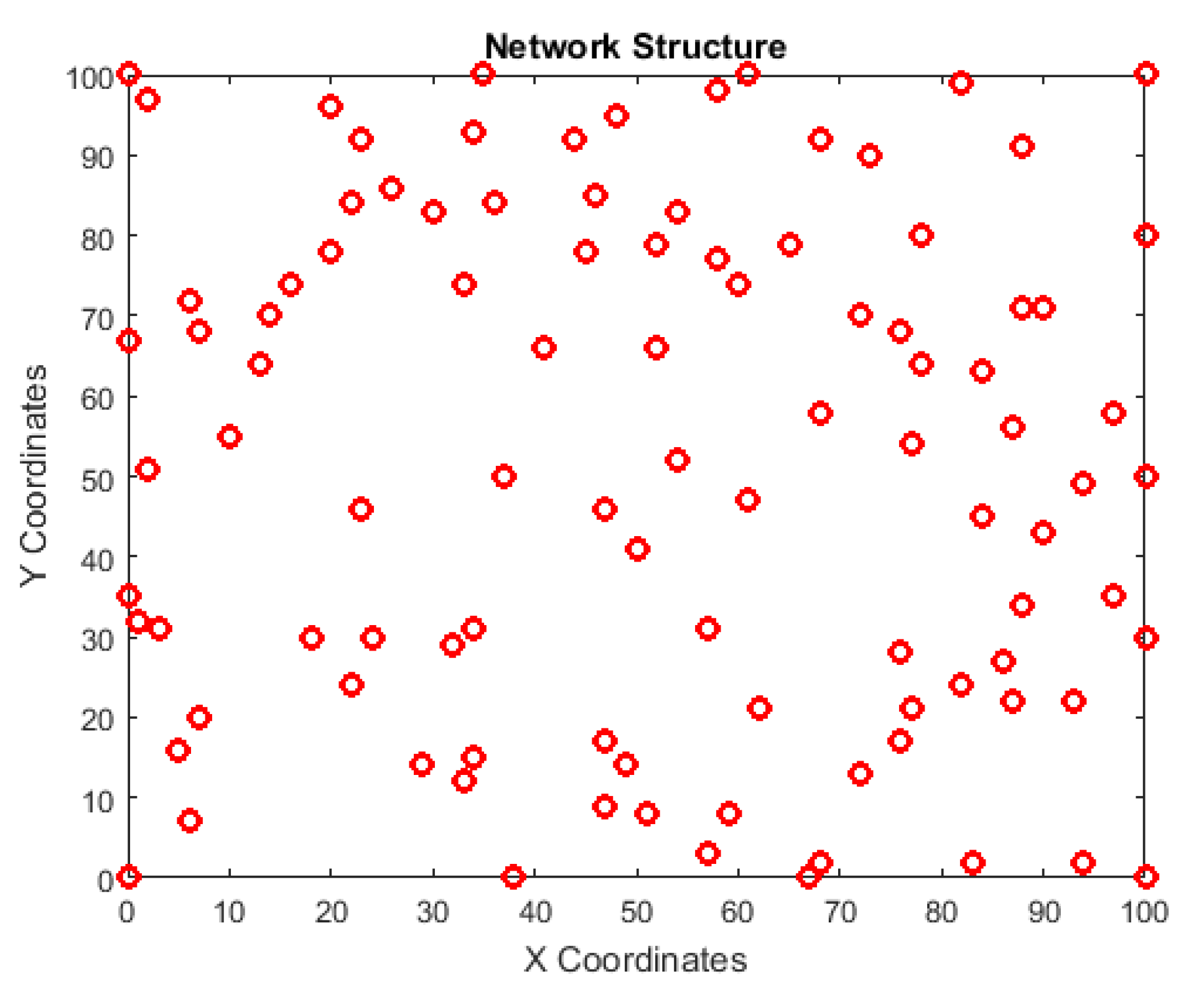
| Target Area | 100 m × 100 m |
| Sensor Nodes (n) | 100 |
| Sensing Radius (Rs) | 8 m |
| Initial Energy of Nodes (E) | 0.1 J (for 90% nodes) 0.2 J (for 10% nodes) |
| Cluster Head Probability (P) | 0.1 |
| Packet Size | 4000 bits |
| Transceiver Energy (ETX, ERX) | 50 × 10−9 J/bit (i.e., 50 nJ/bit) |
| Data Aggregation Energy (EDA) | 5 × 10⁻⁹ J/bit (i.e., 5 nJ/bit) |
| Amplification Energy (Emp), When d > d0 | 0.0013 × 10⁻¹² J/bit/m4 (i.e., 0.0013 pJ/bit/m4) |
| Amplification Energy (Efs), When d ≤ d0 | 10 × 10−12 J/bit/m2 (10 pJ/bit/m2) |
| No. of Rounds (Rmax) | 500 |
| No. of Sink Nodes | 1 (center of the network) |
Publisher’s Note: MDPI stays neutral with regard to jurisdictional claims in published maps and institutional affiliations. |
© 2022 by the authors. Licensee MDPI, Basel, Switzerland. This article is an open access article distributed under the terms and conditions of the Creative Commons Attribution (CC BY) license (https://creativecommons.org/licenses/by/4.0/).
Share and Cite
Sharma, P.; Singh, R.P. Energy-Efficient Deterministic Approach for Coverage Hole Detection in Wireless Underground Sensor Network: Mathematical Model and Simulation. Computers 2022, 11, 86. https://0-doi-org.brum.beds.ac.uk/10.3390/computers11060086
Sharma P, Singh RP. Energy-Efficient Deterministic Approach for Coverage Hole Detection in Wireless Underground Sensor Network: Mathematical Model and Simulation. Computers. 2022; 11(6):86. https://0-doi-org.brum.beds.ac.uk/10.3390/computers11060086
Chicago/Turabian StyleSharma, Priyanka, and Rishi Pal Singh. 2022. "Energy-Efficient Deterministic Approach for Coverage Hole Detection in Wireless Underground Sensor Network: Mathematical Model and Simulation" Computers 11, no. 6: 86. https://0-doi-org.brum.beds.ac.uk/10.3390/computers11060086