A Light Signaling Approach to Node Grouping for Massive MIMO IoT Networks

Abstract

Massive MIMO is one of the leading technologies for connecting very large numbers of energy-constrained nodes, as it offers both extensive spatial multiplexing and large array gain. A challenge resides in partitioning the many nodes into groups that can communicate simultaneously such that the mutual interference is minimized. Here we propose node partitioning strategies that do not require full channel state information, but rather are based on nodes’ respective directional channel properties. In our considered scenarios, these typically have a time constant that is far larger than the coherence time of the channel. We developed both an optimal and an approximation algorithm to partition users based on directional channel properties, and evaluated them numerically. Our results show that both algorithms, despite using only these directional channel properties, achieve similar performance in terms of the minimum signal-to-interference-plus-noise ratio for any user, compared with a reference method using full channel knowledge. In particular, we demonstrate that grouping nodes with related directional properties is to be avoided. We hence realize a simple partitioning method, requiring minimal information to be collected from the nodes, and in which this information typically remains stable over the long term, thus promoting the system’s autonomy and energy efficiency.

1. Introduction

It is clear by now that massive multiple-input multiple-output (MIMO) is a key technology for achieving high capacity in broadband wireless networks, and it is currently being deployed to this end in expanding 5G networks. The use of many electronically steerable service antennas at the base station facilitates aggressive spatial multiplexing to tens of user equipment nodes. This enables a substantial increase in the link reliability experienced by a particular node. In situations where the massive MIMO array is required to simultaneously serve a very large number of nodes, there arises the challenge of first grouping and then scheduling these nodes for transmission. This is particularly important for the massive machine-type communication (mMTC) use case, where extremely large numbers of nodes may be present within the same geographical area served by the base station [1].

In this paper, we propose a node grouping method based on directional properties of the nodes’ channels that are stable over long periods and so do not need to be updated at the rate of the coherence time of the channel. This reduces the signaling overhead and makes our method suitable for use as a precursor to node scheduling for energy-constrained Internet of Things (IoT) nodes with infrequent transmissions. We formulate this as an optimization problem using mixed-integer programming. We then develop an efficient approximation algorithm to solve this problem much faster than is possible using the optimization process. Our results show that both our optimization and approximation provide superior performance in terms of the minimum signal-to-interference-plus-noise ratio (SINR) in comparison to a reference method based on grouping nodes by their instantaneous signal strength, that is, received power, taking into account both small and large-scale fading. The reference method requires full small-scale channel state information (CSI); however, the dominant power consumption of IoT nodes is due to transmission, as shown in [2]. Hence, sending pilot sequences to learn small-scale CSI, prior to data, would consume too much energy. In contrast, less time-varying information could be reused without the need to relearn the channel for each uplink message.

The contributions of this paper are:

• A node partitioning method for massive MIMO systems based on simple directional characteristics of the nodes’ channels, namely, dominant direction and angular spectrum spread, allowing for stable partitioning over a long time period with minimal signaling by the node devices. The partitioning is complete in the sense that every node belongs to a group, so that all nodes are served.
• A formulation of the node partitioning problem using directional channel characteristics as an optimization problem using mixed integer programming.
• An efficient approximation algorithm to solve the problem that runs in $O\left(n\log n\right)$ time, where n is the number of nodes.
• A numerical evaluation of the optimization problem and the approximation algorithm using network examples generated with a suitable channel model, showing similar performance for our partitioning method compared to using full channel information.

The rest of this paper is organized as follows. Section 2 introduces and motivates our node grouping approach. Section 3 then discusses related work on node partitioning and scheduling in massive MIMO systems. Next, Section 4 details our problem setting and defines the node partitioning problem. The partitioning problem is then formulated as a mixed-integer optimization problem in Section 5, and our approximation algorithm to solve this problem more efficiently is given in Section 6. We present our numerical evaluation of the optimization problem and the approximation algorithm in Section 7. Finally, in Section 8, we conclude this paper and discuss future work.

2. Motivation

Many IoT devices are battery-powered and transmit only infrequently, spending the rest of their time in a sleep state. (We recognise that some IoT devices may need to constantly send or receive data; however, here we focus on typical sensors with infrequent transmissions.) Among these devices, there is a large variation in the timescale when transmission and reception need to take place, with the absolute timescale varying from minutes up to tens of days or longer. At such timescales, efficient node grouping and scheduling become difficult, since information about the node traffic and propagation channels can quickly become outdated, unless additional signaling is introduced, which in turn requires nodes to wake up and transmit more often, consuming more energy.

Node grouping consists of partitioning the nodes into groups such that each group can be accommodated for simultaneous transmission in the same coherence block, resulting in a combination of spatial and time multiplexing. This subsequently allows the scheduling of node groups rather than individual nodes, thus reducing the complexity of the scheduling problem. For low-power IoT devices, this partition should be based on node properties that are stable over a considerable time, so that schedules can cover a reasonable number of transmissions, thus reducing signaling and computation costs for scheduling. In addition, node properties used for grouping must also be informative for network performance. To this end, interference within the node groups should be minimized by exploiting characteristics of propagation channels that remain stable over a long time, ideally at least over some tens of node transmissions, and as long as possible to allow for long scheduling windows. This is the subject of this paper.

One possible candidate for a stable channel property is long-term average signal strength, characterized by the average received power. This property can have a significant impact on the inter-node interference in massive MIMO networks, particularly when simple maximum ratio combining (MRC) is used for precoding  [3]. Furthermore, the average received power can be effectively used for node grouping and scheduling [4]. Nevertheless, inter-node interference can also be strongly affected by the directional properties of the users’ channels. Indeed, measurement campaigns have shown that propagation energy typically features dominant directions, and even in reflective environments, real channel responses are far from the “ideal” independent and identically distributed (i.i.d.) Rayleigh fading channels commonly assumed in theory [5,6,7]. This observation suggests that node partitioning that avoids simultaneously scheduling nodes with propagation energy coming from similar directions can actually prevent inter-node interference to a large extent. It is these solutions that we investigate in this work. In terms of the ergodic sum spectral efficiency, there is naturally a price to pay when reducing inter-node interference through user grouping. However, given the low data rates required by typical IoT applications, energy efficiency is a more important performance metric for this use case than spectral efficiency.

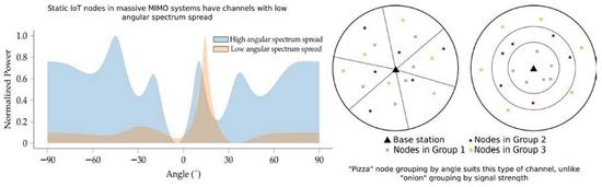
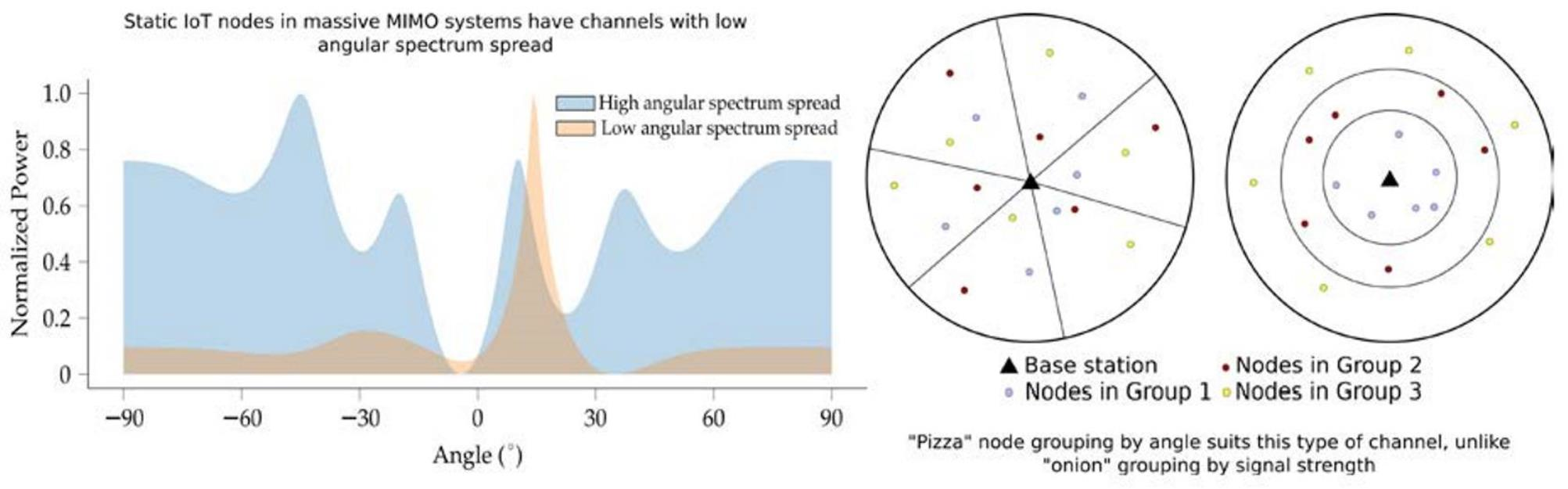
We develop a node partitioning method for massive MIMO systems based on two directional properties of the nodes’ channels, namely, the dominant direction—the angle of arrival of the strongest channel component—and the angular spectrum spread—how widely the channel components are distributed over the possible range of angles of arrival. These properties are stable over larger timescales than the full CSI, which changes according to the channel’s coherence time, and are hence also robust against non-perfect CSI values, easy to collect at the base station with minimal signaling, and correlate with inter-node interference. Specifically, we seek to partition the nodes so as to maximize the minimum angular difference between nodes across multiple different groups according to their angular spectrum spreads.

This approach is analogous to partitioning the nodes within the coverage of a centrally located base station into pizza slices, such that each slice only contains one node from each group (Figure 1, left). This can be compared to an onion ring partitioning approach, where nodes are grouped such that nodes with similar signal strength are placed in the same group. With line-of-sight and free-space propagation, this would result in the groups forming concentric shells, similar to the rings of an onion (Figure 1, right). In more complex channel environments, especially with shadowing or multipath components, the slices and rings will not have such simple geometric shapes as shown in the figure and may even consist of multiple disjointed regions. Although we focus on the pizza approach in this paper, with sufficiently many nodes, the two methods can be readily combined by composition, for example, dividing the nodes into onion rings and then into pizza slices, or vice versa.

3. Related Work

Thus far, there has been limited work on node partitioning in massive MIMO networks in the sense we consider in this paper. There is a substantial body of work on node selection, starting with multiuser MIMO (MU-MIMO) systems [8,9,10,11] even before the advent of massive MIMO. However, the goal of these studies was to choose some subset of the available nodes to be served at a given point in time, typically to maximize the sum rate of the system. Although this is often referred to as node scheduling, it is not true scheduling in that nodes that are not served are not scheduled to be served in future; the nodes are rather partitioned into those that are served and those that are not, with the assumption that as channel conditions change, different nodes will be served over time. We are, however, interested in node partitioning for the purpose of then creating a schedule for all node groups to be served over time. As such, multiple groups are created, and all nodes must be included in at least one group for the partition to be valid. To avoid confusion, we will therefore reserve the term scheduling to mean arranging the service of nodes or node groups over time such that all nodes or groups are eventually served, and use the term selection to mean selecting some subset of nodes for service at a given point in time.

Furthermore, our objective is not to maximize the sum rate of the system. In many IoT use cases, high throughput is not needed. Rather, the aim is often to serve all node demands with minimal energy usage. Here, the rate provided to an individual node does have some relation to this goal, since a high achievable data rate can be used rather to reduce bit errors and thus increase reliability, instead of maximizing throughput. Fewer bit errors mean fewer retransmissions, and thus energy saved. Beyond a certain point, however, nodes do not benefit from a higher SINR as they only have a small amount of data—for example, sensor or control data—to transmit or receive. As such, we aimed to find a node grouping that maximizes the minimum SINR of any node, rather than maximizing the sum rate.

Despite these differences, work on node selection is relevant to our work, since a full node grouping can be regarded as an extension of the binary partitioning of nodes into those that are served and those that are not, and can use similar approaches. We will first discuss the extensive body of work on node selection, and then consider the more limited existing work on scheduling and random access in massive MIMO systems.

3.1. Node Selection for Massive MIMO

When selecting nodes for transmission, many approaches rely on full CSI, such as [12,13,14,15]. However, this is not suitable for our use case since this would require all nodes to first wake up from sleep and then transmit a pilot signal in order for the base station to gather the CSI. For low-power IoT devices, such an approach would consume too much energy to be viable, and does not allow the schedule to be set in advance to provide a defined sleep opportunity and wake-up time.

There is, however, a body of work that performs node grouping based on reduced channel information, which is usually more stable over time. This is often carried out in the context of two-stage beamforming, where pre-beamforming groups are first formed using coarse channel information, and then full precoding takes place after collecting the full CSI for a subset of nodes. Some examples of reduced information that can be used for this purpose are channel quality indicators [16], directional information collected from downlink probing [17], and the covariance matrices of node channels [16,18,19], which can be determined over time by recording statistical channel information. Of particular interest to us are spatial clustering methods [20], sometimes also used in combination with the above techniques.

Joint spatial division and multiplexing (JSDM) [19,21] is one approach that has similarities to ours, although it is not aimed at node partitioning for scheduling. In this method, artificial covariance matrices are constructed based on a set of angles of arrival and angular spreads. Nodes are then clustered into sectors based on the similarity of their channels, for example, by computing the chordal distances of the eigenspaces of nodes’ channel covariance matrices to those of the constructed ones. One key result, proven in [21], is that for a uniformly spaced linear array, JSDM approaches optimality, in terms of maximizing the sum rate, as the number of antennas grows. This is because the node channels, when grouped according to their angles of arrival and angular spreads, form near-orthogonal subspaces. Although the objective of JSDM is different to that of our work, and thus results from JSDM and our method are not comparable, this nonetheless demonstrates the value of node grouping based on directional characteristics, which we also use in our approach.

A key difference between the above work and ours is that we do not wish to select a subset of nodes for service to maximize the sum rate, but rather to serve all nodes over time. An optimal partitioning of nodes where only a subset will be served may be quite different to one where all nodes must be served. In our scenario, nodes with a low signal-to-noise ratio (SNR) or that interfere significantly with other nodes cannot be simply dropped to improve overall performance, but must be accommodated in some group.

A few existing works on node grouping consider other objectives. The authors in [13] grouped nodes into multicast groups according to their interests, with the objective of maximizing minimum throughput. However, in that study, the full CSI was used, which is not feasible for low-power IoT. The authors in [12] focused on IoT, primarily considering the aspect of serving a large number of nodes, rather than low energy usage, since again the full CSI was used and the objective was the maximal sum rate. One interesting aspect of that work was the observation that node groups may overlap, such that each node can be served by more than one group, helping to ensure full coverage. In our work, we use disjoint node groups, but this could be extended to overlapping groups in the future, for example, for nodes that have a higher traffic demand or poor SINR. The authors in [16] performed node selection as in the other work above; however, this was carried out in combination with fair scheduling, to avoid the starvation of nodes that would otherwise be repeatedly not selected. This still did not provide a predictable schedule that would allow a node to sleep until its appointed service time, since nodes were still selected dynamically in each time slot.

3.2. Node Scheduling and Random Access for Massive MIMO Systems

There is also some, albeit limited, existing work on node scheduling for massive MIMO networks. Because massive MIMO systems serve multiple nodes simultaneously, such scheduling inherently requires the creation of node groups, although the groups do not necessarily need to be disjoint. In [4], joint node scheduling and transmission power control was performed for nodes with heterogeneous traffic demands. However, in that study, information about the traffic queues at each node was required, which increases the signaling needed and thus the energy cost. The authors in [22] examined fair scheduling in massive MIMO systems, but provided an analysis of the achievable fair rate, rather than a solution for actually performing scheduling.

Some work has also investigated random access for IoT devices in massive MIMO systems [23,24,25,26,27]. Random access is a promising solution for IoT scenarios with sporadic and unpredictable traffic. However, in cases where there is a high level of contention, random access can lead to collisions, which induce retransmissions and increase energy costs, while further increasing the contention for the channel. Scheduled access also provides more predictable performance, which can be important for some applications, and is more suitable for predictable and/or periodic traffic.

Nevertheless, random access protocols could be combined with our node grouping method, by allowing entire node groups to wake up during a limited period, in which they would be served through random access. Using an intelligent node grouping such as we propose thus also reduces the collision probability within each group and increases the chances of distinguishing colliding transmissions through techniques such as successive interference cancellation. Alternatively, our node grouping method could be used as the precursor to any scheduling algorithm. In both cases, node grouping simplifies network control, since devices can be orchestrated at the group level instead of addressing each individual device, and using node groups for channel access provides for predictable and extended sleep opportunities.

4. Scenario and Problem Definition

We consider a single-cell network with the base station equipped with a large, central antenna array and a number of single-antenna IoT nodes. Here we consider static node devices, and they could be placed in different environments (urban, indoors, rural, etc.), with the cell size varying according to the environment. Although the devices themselves do not move, there may nonetheless be some movement in the environment, for example, people walking around.

Here, we provide a brief overview of massive MIMO transmission, the technology underlying our work. For more details, see [3]. In a massive MIMO system, transmission is established according to the coherence blocks of the channel. A coherence block is a time-by-frequency region in which the channel is constant to within some small margin of error. Within each coherence block, nodes transmit pilot signals in order for the base station to determine the CSI and thus allow data transmission and reception. We consider a time-division duplex (TDD) massive MIMO system, relying on channel reciprocity within each coherence block, and hence not requiring downlink pilots.

In each coherence block, a number of nodes are served simultaneously, for either uplink or downlink transmission, or both. The number of nodes that may be served in each coherence block is limited by either the number of available pilot signals—since each node must be allocated a pilot in order to transmit or receive in the block—or by the inter-node interference, or both. The interference between nodes depends on both the combination of their channels and the precoding scheme used. In this work, we focus on MRC as precoding as it can realize power-efficient spatial multiplexing of devices [3], based on the CSI that is acquired in the TDD-based massive MIMO operation.

In scenarios in which the number of nodes exceeds the number that can be served simultaneously in one coherence block, node grouping becomes necessary, such that each group can be accommodated in a single coherence block. After grouping, node groups can then be scheduled by assigning coherence blocks to them such that the traffic demands of all nodes in the group are satisfied. In this paper, we do not consider scheduling, but rather focus on the node partitioning problem.

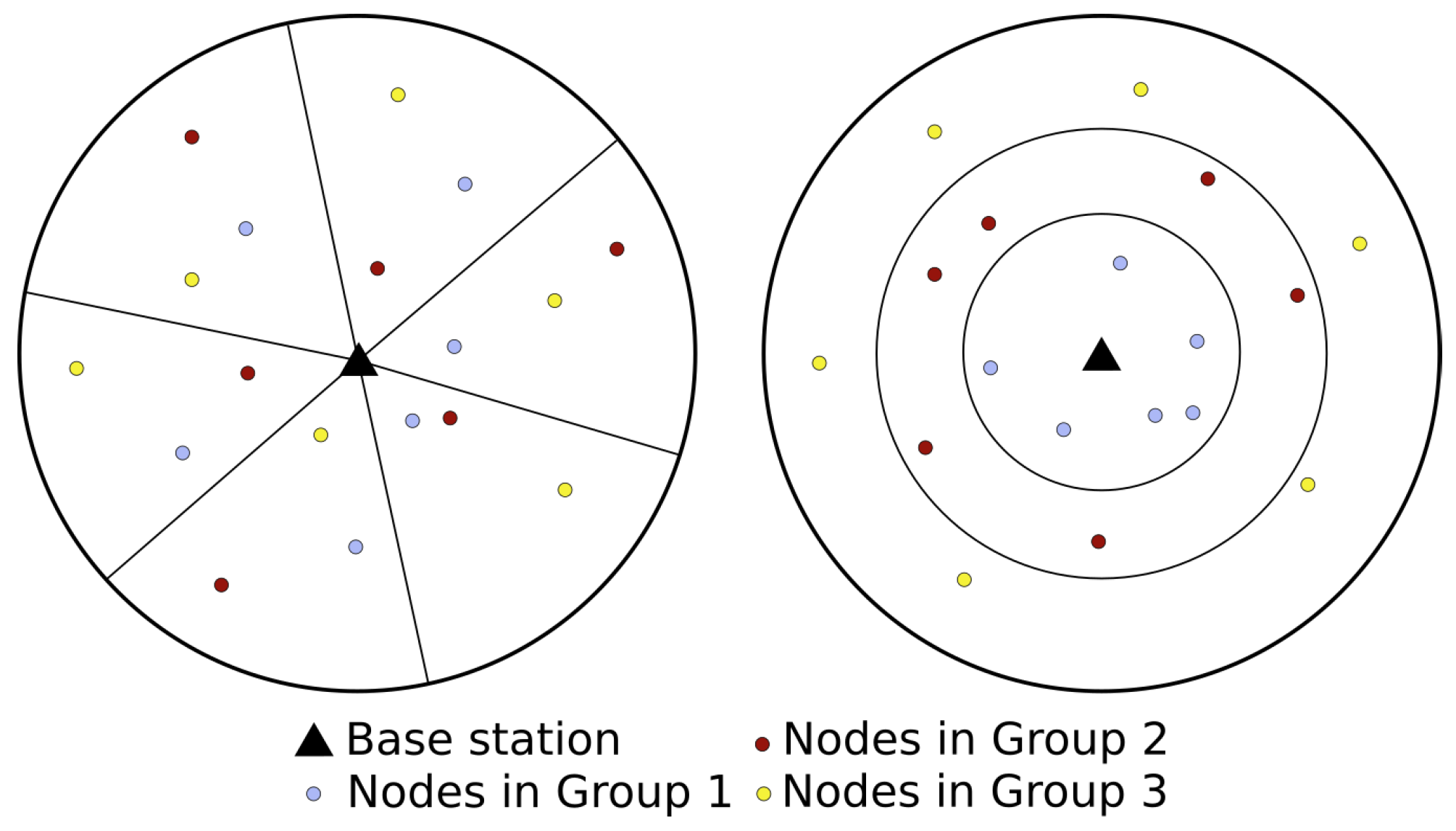
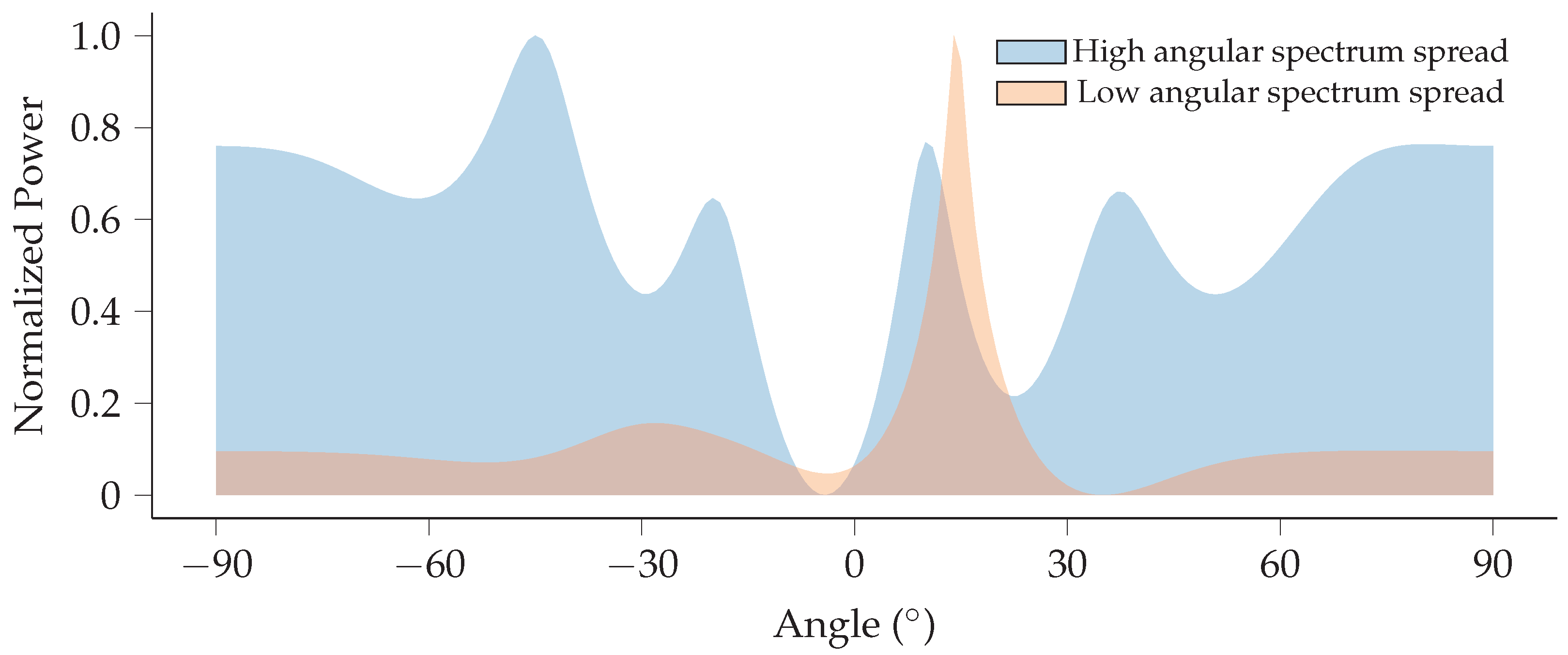
In this work, we perform node grouping based on two directional characteristics of the node channels. The first is the dominant propagation direction, that is, the direction from which the dominant component of a given node’s channel arrives at the base station. The second characteristic we use is the angular spectrum spread—how much the power of the node’s channel, as received by the base station, is spread over the angular domain. A low angular spectrum spread thus implies a channel where the power is largely focused in the dominant direction, whereas a large angular spectrum spread indicates a channel with either multiple strong components or a main component that is spread over a wide angle, or both. Examples of channels with low and high angular spectrum spreads are shown in Figure 2.

For static nodes, these two characteristics of the channel will remain stable over a long period of time, as demonstrated in [28,29]. If there is a line-of-sight component present, this will typically constitute the dominant component, and its direction will not change unless shadowing occurs to block it. Even in cases without a line-of-sight component, there may be one or more strong multipath components, and their directions will similarly be stable in the absence of variable shadowing. The angular spectrum spread is influenced by the number and variety of multipath components. If there are many, the channel is effectively “spread out” over a wider range of angles, leading to a high angular spectrum spread. This means that even if the angles of arrival of individual multipath channel components change, the overall angular spectrum spread will again be relatively stable.

Not only are these directional characteristics stable over time, but they can also be measured at the base station antenna array without requiring too much complex processing [30,31,32]. Moreover, the directional properties of the nodes’ channels are critical for the performance that can be obtained, in terms of the data rate and/or bit error rate. With MRC specifically, the energy of a transmission (on the downlink) is focused at the target node; however, since this focusing is imperfect, especially in the presence of imperfect CSI, interference is caused in relation to nearby nodes. This means that grouping nodes in such a way as to spread out the nodes by angle leads to improved SINRs for the nodes. For these reasons, node partitioning based on directional channel characteristics has the potential to provide a simple partitioning method with minimal information collected from node devices, thus allowing them to sleep longer, transmit less, and save energy.

5. Optimization

We now present the node grouping optimization problem. We begin by detailing the system model and notation, and then describe our mixed-integer programming optimization formulation. The notation is summarized in

Table 1. Notation.

Symbol	Explanation
$\mathcal{K}$	set of nodes
$\theta \left(k\right)$	dominant direction of node $k\in \mathcal{K}$
P	number of pilots in each coherence block
$\mathcal{G}$	set of scheduling groups
$u_{kg}$	whether or not node $k\in \mathcal{K}$ is placed in group $g\in \mathcal{G}$
$\mathcal{P}$	the set $\{1,...,P\}$, $P\in \mathbb{N}$
$Y_{kg}^p$	whether or not node $k\in \mathcal{K}$ is the pth node in group $g\in \mathcal{G}$, $p\in \mathcal{P}$
$t_g^p$	angle of the pth node in group $g\in \mathcal{G}$, $p\in \mathcal{P}$
$T_g$	angle of the last node in group $g\in \mathcal{G}$
$d_g^p$	p-th angular difference of nodes in group $g\in \mathcal{G}$, $p\in \mathcal{P}$
B	min-max angular difference across groups
$\sigma \left(k\right)$	angular spectrum spread of node $k\in \mathcal{K}$
$s_g^p$	angular shift of the pth node in group $g\in \mathcal{G}$, $p\in \mathcal{P}$
$S_g$	angular shift of the last node in group $g\in \mathcal{G}$
$m_g^p$	whether or not the pth node in group $g\in \mathcal{G}$ is the last node in the group, $p\in \mathcal{P}$

.

5.1. System Model

We have a set of nodes (IoT devices) $\mathcal{K}$ served by a massive MIMO base station. Each node $k\in \mathcal{K}$ has a dominant direction of its signal, as defined in the previous section, denoted by $\theta \left(k\right)$ and measured in radians clockwise from a designated reference direction (e.g., due north). In the following, if not otherwise specified, all other angles are also defined as clockwise from this reference direction. The dominant direction does not necessarily represent the direction to the physical location of the node; it could also be a signal component reflected one or more times from an object in the environment. For our purposes, however, the physical location of the node is less important than the arrival direction of its transmitted signals.

Scheduling of nodes for both uplink and downlink transmission occurs in coherence blocks, such that a given group of nodes should be scheduled for an integer number of blocks. Herein we focus on partitioning the set of nodes $\mathcal{K}$ into groups that can be scheduled together. In each coherence block, there are P available pilot signals, and this thus represents the maximum number of nodes that can be placed in each group.

We define a set of scheduling groups $\mathcal{G}$, where each group may contain at most P nodes. The groups do not necessarily need to contain the same number of nodes, and some groups may even be empty. The partitioning of nodes into groups is represented by binary decision variables $u_{kg}$, $k\in \mathcal{K}$, $g\in \mathcal{G}$, equal to 1 if and only if node k is placed in group g. Within each group, the nodes are ordered by their dominant directions. We therefore define binary variables $Y_{kg}^p$, $k\in \mathcal{K}$, $g\in \mathcal{G}$, $p\in \mathcal{P}=\{1,\cdots ,P\}$, where $Y_{kg}^p=1$ indicates that k is the pth node in g. If a given group g contains fewer than P nodes, some $Y_{kg}^p$ will be zero for all $k\in \mathcal{K}$. The angle of the pth node in group g is given by the continuous variable $t_g^p$, with $t_g^p=0$ if group g contains fewer than p nodes.

We next introduce continuous variables $d_g^p$, $g\in \mathcal{G}$, $p\in \mathcal{P}$ to represent the differences in angle between adjacent nodes in each group. For p less than the number of nodes in group g, we thus have $d_g^p=t_g^{p+1}-t_g^p$ for $p<P$. Variable $d_g^P$ is used to represent the angular difference between the last and the first nodes node in group g, thus completing the circle, regardless of the total number of nodes in the group, that is, even if group g has fewer than P nodes. Finally, we define the continuous variable B, which represents the maximum of the minimum angular differences in all the groups, and this will constitute our objective function.

In addition to the dominant direction, we use the angular spectrum spread to inform node grouping (see Section 4). In massive MIMO systems, the signal from a node with a large angular spectrum spread is more easily distinguished from other signals, even from nodes that have similar dominant directions, since there are more multipath components to use to differentiate the channels. This means that a node with a large angular spectrum spread causes less interference to nearby (in angle) nodes, and so can be more readily placed in a group with them.

For the purposes of partitioning the nodes into scheduling groups, we model the angular spectrum spread by considering an angular tolerance allowing nodes to symbolically “move” around a circle from their initial positions (given by their dominant directions), in such a way as to increase their angular differences to the neighboring nodes in the group. We first define the normalized angular spectrum spread of a node $k\in \mathcal{K}$, $\sigma \left(k\right)$, where $0\le \sigma \left(k\right)\le 1$. Here, $\sigma \left(k\right)=0$ means that the node’s signal is entirely composed of a component coming from its dominant direction, with no angular spectrum spread. In such a case, the node will not be permitted to move from its initial direction $\theta \left(k\right)$. On the other hand, $\sigma \left(k\right)=1$ means that the dominant direction cannot be distinguished at all: the node’s signal comes evenly from all directions, i.e., we have an i.i.d. Rayleigh fading channel. Such a node may symbolically move freely to any angle around the circle, and this shift is represented by the decision variable $s_g^p$, for the pth node in group $g\in \mathcal{G}$. Of course, in reality the nodes do not move; shifting the nodes on the circle corresponds rather to reducing the influence of the angular proximity of two nodes if their angular spectrum spreads allow their channels to be distinguished by the base station anyway, equivalent to if they had a larger angular difference in the first place.

Lastly, we will use decision variables $m_g^p$ to indicate whether or not the pth node in group $g\in \mathcal{G}$ is the last node in this group. This will allow us to compute variables $T_g$ and $S_g$, the angle and angular shift of the last node in each group $g\in \mathcal{G}$, respectively. These will be used to correctly compute the angular differences to neighboring nodes, since the last node in each group is a special case, as one of its neighbors is the first node in the group as the nodes are placed on a circle.

5.2. Formulation

We can now formulate the optimization problem, which we will refer to as Maximization of Minimum Angular Difference (MMAD) as follows.

$$\begin{array}{ccc}\hfill max& B\hfill & \hfill \end{array}$$

(1)

$$\begin{array}{ccc}\hfill & \sum _{g\in \mathcal{G}}{u}_{kg}=1,\hfill & \hfill k\in \mathcal{K}\end{array}$$

(2)

$$\begin{array}{ccc}\hfill & \sum _{k\in \mathcal{K}}{u}_{kg}\le P,\hfill & \hfill g\in \mathcal{G}\end{array}$$

(3)

$$\begin{array}{ccc}\hfill & \sum _{p\in \mathcal{P}}{Y}_{kg}^p=u_{kg},\hfill & \hfill k\in \mathcal{K},g\in \mathcal{G}\end{array}$$

(4)

$$\begin{array}{ccc}\hfill & \sum _{k\in \mathcal{K}}{Y}_{kg}^p\le 1,\hfill & \hfill p\in \mathcal{P},g\in \mathcal{G}\end{array}$$

(5)

$$\begin{array}{ccc}\hfill & \sum _{k\in \mathcal{K}}{Y}_{kg}^p\le \sum _{k\in \mathcal{K}}{Y}_{kg}^{p+1},\hfill & \hfill p\in \mathcal{P}\setminus \left\{P\right\},g\in \mathcal{G}\end{array}$$

(6)

$$\begin{array}{ccc}\hfill & t_g^p=\sum _{k\in \mathcal{K}}\theta \left(k\right)Y_{kg}^p,\hfill & \hfill p\in \mathcal{P},g\in \mathcal{G}\end{array}$$

(7)

$$\begin{array}{ccc}\hfill & t_g^p\le t_g^q+2\pi \left(1-\sum _{k\in \mathcal{K}}{Y}_{kg}^p\right),\hfill & \hfill p,q\in \mathcal{P},p<q,g\in \mathcal{G}\end{array}$$

(8)

$$\begin{array}{ccc}\hfill & s_g^p\le \pi \sum _{k\in \mathcal{K}}\sigma \left(k\right)Y_{kg}^p,\hfill & \hfill p\in \mathcal{P},g\in \mathcal{G}\end{array}$$

(9)

$$\begin{array}{ccc}\hfill & T_g\ge t_g^p,\hfill & \hfill p\in \mathcal{P},g\in \mathcal{G}\end{array}$$

(10)

$$\begin{array}{ccc}\hfill & T_g\le \sum _{p\in \mathcal{P}}{t}_g^p{m}_g^p,\hfill & \hfill g\in \mathcal{G}\end{array}$$

(11)

$$\begin{array}{ccc}\hfill & S_g=\sum _{p\in \mathcal{P}}{s}_g^p{m}_g^p,\hfill & \hfill g\in \mathcal{G}\end{array}$$

(12)

$$\begin{array}{ccc}\hfill & \sum _{p\in \mathcal{P}}{m}_g^p=1,\hfill & \hfill g\in \mathcal{G}\end{array}$$

(13)

$$\begin{array}{ccc}\hfill & d_g^p\le t_g^{p+1}-t_g^p+s_g^{p+1}+s_g^p,\hfill & \hfill p\in \mathcal{P}\setminus \left\{P\right\},g\in \mathcal{G}\end{array}$$

(14)

$$\begin{array}{ccc}\hfill & d_g^P\le t_g^1+2\pi -T_g+s_g^1+S_g,\hfill & \hfill p\in \mathcal{P}\setminus \left\{P\right\},g\in \mathcal{G}\end{array}$$

(15)

$$\begin{array}{ccc}\hfill & d_g^p\le \pi ,\hfill & \hfill p\in \mathcal{P},g\in \mathcal{G}\end{array}$$

(16)

$$\begin{array}{ccc}\hfill & B\le d_g^p+\pi \left(1-\sum _{k\in \mathcal{K}}{Y}_{kg}^p\right),\hfill & \hfill g\in \mathcal{G}\end{array}$$

(17)

$$\begin{array}{ccc}\hfill & B\le d_g^P,\hfill & \hfill g\in \mathcal{G}\end{array}$$

(18)

$$\begin{array}{ccc}\hfill & u_{kg},Y_{kg}^p,m_g^p\in \mathbb{B};t_g^p,s_g^p,T_g,S_g\in \mathbb{R};B,d_g^p\in {\mathbb{R}}^{+},\hfill & \hfill p\in \mathcal{P},g\in \mathcal{G}.\end{array}$$

(19)

The objective function, (1), maximizes the minimum angular difference, adjusted for the angular spectrum spread, between any two nodes in any one group, based on their symbolic placement around a circle. We assume that performance, in terms of achievable SINR, will in general improve for any given node the greater the angle between it and its closest neighbors that are scheduled in the same group. However, this relationship is not straightforward for channels with multipath components, since nodes of which the dominant directions lie close to one another may nonetheless have little correlation between their channels if they have significant power in multipath components with different angles of arrival. The minimum angular difference that is maximized therefore takes the angular spectrum spread of the nodes’ channels into account, via the constraints that will be explained below.

The first constraint, (2), ensures that each node is placed in exactly one group, and constraint (3) then ensures that the number of nodes placed in each group does not exceed the number of available pilots, P. The decision variables $Y_{kg}^p$ are used to keep track of which group each node is placed in, along with which order it is placed in. Hence, $Y_{kg}^p$ should be set to 1 if node $k\in \mathcal{K}$ is placed in group $g\in \mathcal{G}$ at position $p\le P$, and 0 otherwise. This is enforced using constraints (4) and (5). Constraint (4) requires that exactly one position in group $g\in \mathcal{G}$ be assigned to node $k\in \mathcal{K}$, if the node is placed in that group ($u_{kg}=1$), and that no positions in the group are assigned to it if it was not placed in that group ($u_{kg}=0$). Constraint (5) ensures that at most one node is assigned to each position in each group, i.e., a strict ordering is imposed in which two or more nodes cannot occupy the same position. Finally, constraint (6) prevents gaps in the node ordering for each group, that is, no position in the group may be filled until all the preceding positions are filled.

The next three constraints determine the angles and angular tolerances of each node in each group. Constraint (7) sets the angle of each node position in each group to be the dominant direction of the node assigned to that position, through the decision variable $t_g^p$. Constraint (8) ensures that nodes are assigned positions in groups in the order of their dominant directions, that is, a node with a higher angle for its dominant direction may not be placed earlier in a group than a node with a lower angle. The second term on the right-hand side is used to cancel this constraint when a position in a group is empty, that is, not assigned to any node. Such empty positions must occur at the end of the group, thanks to constraint (6). Constraint (9) determines the angular tolerance for each position in each group, up to a maximum of the angular spectrum spread for the node assigned that position. This angular tolerance gives the range within which the node’s angular position can be adjusted.

Because the nodes are symbolically placed on a circle, in which an angle of $2\pi$ is equivalent to an angle of 0, the last node in each group must be treated differently. For the purpose of computing the objective, angular differences between each successive pair of nodes in each group are considered, and additionally the angular difference from the last node back around the remainder of the circle to the first node must be included. Constraints (10)–(13) are used to find the angle and angular shift for the last node in each group. The binary decision variable $m_g^p$ is set to 1 for the last position in each group, and 0 otherwise. It is not possible to determine in advance which is the last position in any given group, since the groups may have different numbers of nodes assigned to them.

Constraint (13) forces only one position in each group to be selected as the last. To make sure the one selected is indeed the last, and to obtain the angle of the node in the last position, constraints (10) and (11) are used. Constraint (10) requires that the angle of the last position in each group $g\in \mathcal{G}$, $T_g$, be at least as large as all angles in the group $t_g^p$. Meanwhile, constraint (11) requires that $T_g$ be no more than the angle of the node selected by the variable $m_g^p$. In this way, $m_g^p$ can only feasibly be 1 for the last position in the group. Similarly, variable $S_g$ is set to the angular shift of the last node in the group via constraint (12).

Next, the angular differences between the nodes in each group need to be computed, in constraints (14)–(16). Constraint (14) sets variable $d_g^p$ to be, at most, the angular difference between the nodes at positions p and $p+1$ in group g, taking into account their angular tolerances. Since the objective is a maximization function, equality will be achieved here for any angular differences that can affect the objective. Constraint (15) similarly takes the angular difference between the last and first positions in each group, thus closing the circle. Note that the variable $d_g^P$ is used for this last angular difference, regardless of whether or not the last occupied position in the group is P or a lower position, due to the group having fewer than P nodes assigned to it. Constraint (16) limits all angular differences to be, at most, $\pi$, since any difference greater than this would imply a smaller angular difference if measured in the opposite direction around the circle.

We are now ready to compute the objective function using constraints (17) and (18). These constraints set the objective function value, represented by variable B, to the minimum angular difference of any pair of nodes in any group. Here, again, the last position in each group must be treated separately (constraint (18)). In constraint (17), the second term on the right-hand side cancels the constraint for any positions to which no node has been assigned. Finally, the last three constraints in the formulation provide the domains for each of the decision variables.

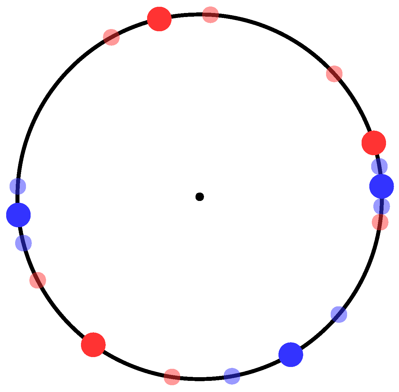
An example problem instance and solution are shown in Figure 3. In this instance, six nodes are partitioned into two groups. The nodes’ angular shift ranges are indicated in the figure by the smaller, semi-transparent circles. For this problem, most nodes’ ranges do not overlap and so do not affect the solution; the nodes are placed into the two groups in an alternating fashion. However, two of the nodes’ ranges overlap, and in this case the nodes are grouped “out of order”, as they are able to shift within their ranges in order to achieve larger angular differences to the other nodes.

Auxiliary Variables

To resolve the bilinearities in constraints (11) and (12), we need to introduce auxiliary variables $v_g^p=t_g^p{m}_g^p$ and $z_g^p=s_g^p{m}_g^p$, $p\in \mathcal{P}$, $g\in \mathcal{G}$, and add the following constraints to MMAD.

$$\begin{array}{ccc}\hfill & v_g^p\le t_g^p;v_g^p\le 2\pi m_g^p;v_g^p\ge t_g^p+2\pi \left(m_g^p-1\right),\hfill & \hfill p\in \mathcal{P},g\in \mathcal{G}\end{array}$$

(20)

$$\begin{array}{ccc}\hfill & z_g^p\le s_g^p;z_g^p\le \pi m_g^p;z_g^p\ge s_g^p+\pi \left(m_g^p-1\right),\hfill & \hfill p\in \mathcal{P},g\in \mathcal{G}.\end{array}$$

(21)

Constraint (11) is then replaced with $T_g\le {\sum }_{p\in \mathcal{P}}{v}_g^p,g\in \mathcal{G}$, and constraint (12) with $S_g={\sum }_{p\in \mathcal{P}}{z}_g^p,g\in \mathcal{G}$. This renders the formulation a valid mixed-integer programming problem, but is otherwise equivalent to MMAD.

6. Approximation Algorithm

Solving MMAD to optimality may require more time than is available to partition the nodes and schedule their transmissions. As we will see in Section 7.2, the time to find an optimal solution increases exponentially with the size of the problem, and for many IoT scenarios the number of nodes can be very large. In some cases, it may nonetheless be possible to use optimal solutions, since it is also often the case that IoT devices transmit only infrequently; for example, sensor data may be gathered once every hour or day, which, depending on the number of nodes, may allow enough time to solve the optimization problem.

In many cases, there will not be sufficient time and/or computational resources available or justifiable to find an optimal solution before it is needed, especially in view of the current trend of moving more intelligence deeper in the network. To address such scenarios, we created a suboptimal algorithm based on the same principles as the optimization formulation. This algorithm is efficient and can be used even for scenarios with many nodes that need to be partitioned and scheduled frequently. The algorithm is listed in Algorithm 1. Since the domain of our optimization (the circle) is finite, there is an inherent additive bound on the solution as compared with the optimal solution: the deviation of the solution provided by Algorithm 1 from the optimal solution cannot be greater than $\pi$, and hence we refer to it as an approximation algorithm in the following.

Algorithm 1: Approximation algorithm for node partitioning based on dominant direction and angular spectrum spread.

The basic idea of the approximation algorithm is to sort the nodes by angle, that is, by their dominant directions but also taking into account their angular spectrum spreads, and then assign a group to each node sequentially in a round robin fashion. In this way, nodes in the same group will be as far away as possible from each other in terms of their position in the sequence, although not necessarily in terms of their angles, since the solutions produced by this algorithm are suboptimal in general.

To take the angular spectrum spreads into account, an angular shift is computed for each node $k\in \mathcal{K}$ as $\pi \sigma \left(k\right)$, where $\sigma \left(k\right)$ is the normalized angular spectrum spread of k. This is similar to constraint (9) in the optimization. The angular shift is first subtracted from each node’s dominant direction (line 2), and the node with the minimal resulting angular position is taken as the first node and assigned to the first group (lines 5–6). Then, for the remaining nodes, the angular shift is added to each node’s dominant direction (line 3) and the nodes are again sorted by the resulting angle (line 9). Nodes are taken from the head of the resulting list one at a time in order and assigned a group in a round robin fashion (lines 10–15), that is, cycling through the groups in order and assigning one node to each before repeating the process.

The most complex operation in the algorithm is sorting the nodes, which is performed twice sequentially. Efficient sorting algorithms, such as quick sort and merge sort, can perform this operation in $O\left(KlogK\right)$ time, where $K=\left|\mathcal{K}\right|$ is the number of nodes to be sorted. The two sequential for loops each have a complexity of $O\left(K\right)$, which is lower than that of the sorting operation so it does not increase the overall complexity class. All other operations are basic operations that are executed in $O\left(1\right)$ time. Thus, the total computational complexity of the approximation algorithm is $O\left(KlogK\right)$.

It should also be noted that in cases where the angular spectrum spreads are low, such that the resulting angular shifts are lower than the angular differences between nodes’ dominant directions for most nodes, the list of nodes will already be nearly sorted, assuming it is initially provided in the order of the nodes’ dominant directions. In this case, the complexity could be reduced even further by using bubble sort, which has good performance of $O\left(K\right)$ for an almost-sorted list where no node is out of place by more than one position. In such a case, the complexity of our approximation algorithm also becomes $O\left(K\right)$. Since node partitioning based on angles, as proposed in this paper, is intended for cases where node channels have a strong dominant component and thus interference correlates strongly with the directional characteristics of the channel, cases where the angular spectrum spread is low enough to use bubble sort are quite likely to occur. Checking whether a given problem instance fulfils the needed conditions can be performed in $O\left(K\right)$ time, for example, by performing the first pass of bubble sort and, in case the list is not yet sorted, switching to quick sort or merge sort. Thus, this added optimization for such cases can be included at no additional cost in terms of computational complexity.

7. Numerical Evaluation

We conducted a numerical evaluation to test the performance of our optimization and approximation algorithm, along with two reference algorithms, one of which uses the full CSI, on randomly generated instances of our problem scenario, consisting of a set of single-antenna nodes and an accompanying channel matrix. We compared the performance of the algorithms in terms of the achieved minimum, maximum, and average SINR. We also compared the performance of our approximation with the optimal solution in terms of the proportion of the optimal objective function value obtained by the approximation. All the source code for our implementations of the optimization problem, approximation algorithm, channel model, and experiments is available online [33].

The parameters for our numerical evaluation are given in

Table 2. Parameters for the numerical evaluation.

Parameter	Symbol	Value
Number of nodes	$\left|\mathcal{K}\right|$	$15\cdots 36$, step 3
Number of instances for each number of nodes	-	20
Number of pilots	P	12
Number of groups	$\left|\mathcal{G}\right|$	3
Number of base station antennas	M	100
Type of antenna array	-	Uniform rectangular array
Precoding	-	Maximum ratio combining
Carrier frequency	-	$2.47$$\mathrm{G}$$\mathrm{Hz}$
Number of channel clusters	$N_{\mathrm{cl}}$	4
Number of channel components per cluster	$N_{\mathrm{ray}}$	10
Distribution of cluster central angles	-	Uniform 45–135 degrees
Distribution of component angles within each cluster (vertical and horizontal)	-	Exponential, $\mu =7.5$ degrees
Component small scale fading distribution	-	Complex normal, $\mu =0$, $\sigma =1$
Signal-to-noise ratio (for all nodes)	-	20 dB

. We generated instances consisting of between 15 and 36 nodes, along with a massive MIMO base station with 100 antennas, and 12 pilots available in each coherence block. These base station parameters are based on the Lund University massive MIMO (LuMaMi) testbed [34,35]. The numbers of nodes and pilots were also chosen such that there were always fewer pilots than nodes, necessitating node grouping.

We partitioned the nodes into three groups, and so as the number of nodes increased, the number of nodes per group increased accordingly. The number of nodes per group is the most important parameter for determining the achievable SINR, since with more nodes per group the density of nodes is greater and the angular differences between them are lower. Meanwhile, the overall number of nodes is the most important parameter in terms of the running time of the partitioning algorithms.

For each number of nodes, we generated and tested 20 problem instances. The instances were generated using a channel model based on the Saleh–Valenzuela model [36] and its adaption to MIMO channels [37]. The channel model and problem instance generation will be further detailed in Section 7.1. As an output, the model produces the dominant direction and angular spectrum spread for each node, along with the complete channel matrix, giving the channel from each node to each base station antenna.

Using the dominant directions and angular spectrum spreads, we then ran our optimization MMAD, given in Section 5.2, on each problem instance. For this purpose, we used the AMPL modeling language [38], along with the CPLEX optimization solver [39], and the optimization was run on a 12-core server with $2.2$ GHZ Intel Xeon ES-2420 CPUs and 24 GiB RAM. The optimal solution was then compared with three other node partitioning algorithms. An overview of the partitioning algorithms is given in

Table 3. Partitioning Algorithms Tested.

Node Partitioning Method	Description
Optimal Solution	Solving MMAD to optimality.
Approximation algorithm	Algorithm 1
Clumped partitioning	Groups nodes with similar directional properties together. Worst-case scenario using directional properties.
Power partitioning	Groups nodes with similar received power at the base station together. Partitioning suitable for use with max-min fair power control. Requires full CSI.

. The first comparison algorithm was our approximation algorithm, given in Algorithm 1.

The second comparison algorithm, which we will refer to as clumped node partitioning, is intended to represent a worst-case scenario in which nodes whose channels have similar directional properties are grouped together. In this algorithm, the nodes are first sorted according to their dominant directions. Then the first $N=\frac{\left|\mathcal{K}\right|}{\left|\mathcal{G}\right|}$ nodes are placed in the first group, the next N nodes in the next group, and so on, until all nodes have been assigned a group. The computational complexity of this algorithm is $O\left(\right|\mathcal{K}\left|log\right(\left|\mathcal{K}\right|)$, since it first sorts the nodes and then performs a sequential group assignment for each node. In our test instances, the number of nodes is always divisible by the number of groups, so there will be no nodes left over with this procedure, and all groups will contain the same number of nodes. Clumped partitioning gives an indication of the detriment to performance that might be caused by a poor node partition with respect to the directional channel properties we consider.

The third comparison algorithm, called power partitioning, uses the entire channel matrix as an input, rather than only the directional properties of the node channels, and thus is used as a comparison against the case where the full channel information is obtained before partitioning. To the best of our knowledge, no existing methods from the literature take a similar approach to ours in terms of avoiding the collection of CSI and instead using other properties. Collection of the full CSI is not feasible in practice. This is firstly because it would require partitioning nodes after they have transmitted pilots in the coherence block in which they are to transmit, whereas in reality pilots can only be allocated to nodes after partitioning has been performed. Secondly, in an IoT scenario, the signaling cost for collecting channel information in order to perform partitioning is too high; our aim is to provide a partitioning strategy with low energy usage for the end devices.

Power partitioning sorts the nodes according to the received power of their channels at the base station, and then groups those nodes with similar power levels. Similarly to clumped partitioning, this is achieved by assigning the $N=\frac{\left|\mathcal{K}\right|}{\left|\mathcal{G}\right|}$ nodes with the highest received power to the first group, the next N highest power nodes to the next group, and so on. As for clumped partitioning, the computational complexity is $O\left(\right|\mathcal{K}\left|log\right(\left|\mathcal{K}\right|)$, as power partitioning works in a similar way. This does not include the complexity for collecting and processing the CSI in order to find the received power for each node, since this will depend on the specific implementation for downlink precoding and uplink combining. For MRC precoding, the interference scales with the interfering nodes’ received power [3]. Power partitioning thus provides a reasonably fair partition, in which nodes experience interference only from other nodes with similar received power.

Power partitioning is thus similar to max-min fair power control [40], in which a common SINR is achieved for all users by adjusting their transmission power such that the received power from each user at the base station is equal. In the absence of transmission power control, fair performance—in the form of equal SINR—cannot be achieved exactly; however, power partitioning comes as close as possible using only partitioning. If partitioning were to then be combined with transmission power control, power partitioning would then provide the best conditions for carrying out max-min fair power control, since the users in each group will have as similar received power levels as possible before applying the power control algorithm. For these reasons, power partitioning provides a good comparison algorithm making use of the full CSI for our use case, in which the goal is to maximize the minimum SINR, rather than provide the maximum sum rateas in other user selection algorithms (see Section 3).

Finally, we computed the SINR achieved for each node for the partitions produced by each of the algorithms. Here, the interfering nodes are only those that were placed in the same group, as it is these nodes that will transmit in the same coherence block. We then took the minimum SINR obtained by any node in any group as our primary performance metric; however, we also examined the average and maximum SINR across all the nodes.

7.1. Channel Model

To generate each problem instance, we used the channel model from [37], which is in turn based on the Saleh–Valenzuela model [36]. The model defines the channel matrix $\mathbf{H}$ as

$$\mathbf{H}=\sqrt{\frac{M}{N_{\mathrm{cl}}{N}_{\mathrm{ray}}}}\sum _{i=1}^{N_{\mathrm{cl}}}\sum _{l=1}^{N_{\mathrm{ray}}}{\alpha }_{i\ell }{\Lambda }_{\mathrm{r}}\left({\varphi }_{i\ell }^{\mathrm{r}},{\theta }_{i\ell }^{\mathrm{r}}\right){\Lambda }_{\mathrm{t}}\left({\varphi }_{i\ell }^{\mathrm{t}},{\theta }_{i\ell }^{\mathrm{t}}\right){\mathbf{a}}_{\mathrm{r}}\left({\varphi }_{i\ell }^{\mathrm{r}},{\theta }_{i\ell }^{\mathrm{r}}\right).$$

(22)

The channel matrix $\mathbf{H}$ models the effect of all the nodes’ signals arriving at the M receive antennas of the base station. At the nodes’ side, single antennas are considered. The signals are modeled as multiple components, grouped into $N_{\mathrm{cl}}$ different clusters. Clusters can, for example, be created by objects in the environment that the nodes’ signals are reflected from (possibly multiple times) before arriving at the base station. Each cluster has a central angle of arrival in relation to the base station, around which its $N_{\mathrm{ray}}$ constituent components propagate. The propagation effects (attenuation and phase rotations) are modeled in the complex gain ${\alpha }_{i\ell }$ for each contributing ray. The receive array response is denoted by ${\mathbf{a}}_{\mathrm{r}}\left({\varphi }_{i\ell }^{\mathrm{r}},{\theta }_{i\ell }^{\mathrm{r}}\right)$ and is a function of the antenna array structure, the azimuth, and elevation angles (${\varphi }_{i\ell }^{\mathrm{r}},{\theta }_{i\ell }^{\mathrm{r}}$) of the arriving signal of the ℓth ray in the ith cluster. The expression of the array response for a uniform linear array (ULA) and a uniform rectangular array (URA) can be found in [41]. The antenna element gain of the receive and transmit antennas are denoted by the functions ${\Lambda }_{\mathrm{r}}\left({\varphi }_{i\ell }^{\mathrm{r}},{\theta }_{i\ell }^{\mathrm{r}}\right)$ and ${\Lambda }_{\mathrm{t}}\left({\varphi }_{i\ell }^{\mathrm{t}},{\theta }_{i\ell }^{\mathrm{t}}\right)$, respectively. For isotropic antennas, the antenna element gain is one ($\Lambda =1$), as the gain is independent of the azimuth and elevation angle.

In our experiments, we used four clusters, each with ten components, and the cluster central angles were drawn from a uniform random distribution between 45 degrees and 135 degrees, where 90 degrees is perpendicular to the plane of the URA. The components were distributed around these central angles according to exponential distributions with a mean of $7.5$ degrees, one in each of the vertical and horizontal planes, with a $0.5$ probability of a given component lying in either direction from the central angle in each plane. Each component is subject to small-scale fading as ${\alpha }_{i\ell }$ is following a complex normal distribution with a mean of 0 and a standard deviation of 1. Finally, the node channels are normalized such that the expected power of each node’s signal is 1.

In [37], clusters are generated homogeneously; however, our use case concerns channels that exhibit clear dominant directions [28]. To model this, for each node, we amplified the cluster with the highest power, by multiplying it by a scalar drawn uniformly randomly from the interval $[2.0,6.0]$. This could represent either the line-of-sight part of the node’s channel, or a set of components reflected from a highly reflective surface, if there is no line-of-sight path between the base station and the node. The node channel was then re-normalized to ensure that the expected power was still $1.0$. In this way, we generated channels with a more clear dominant component and lower angular spectrum spread than in [37].

The dominant direction for each node was taken to be the central angle of the dominant cluster. To compute the angular spectrum spread, we used the Rician K-factor, adjusted for the angular distribution of the generated clusters for each node. For each node $k\in \mathcal{K}$, the angular spectrum spread $\sigma \left(k\right)$ was computed as

$$\sigma \left(k\right)=\Psi \left(k\right)\left(1.0-\frac{P\left(C_d\left(k\right)\right)}{{\sum }_{c\in \{\mathcal{C}\left(k\right)\setminus C_d\left(k\right)\}}P\left(c\right)}\right),$$

(23)

where $\mathcal{C}\left(k\right)$ is the set of clusters in node k’s channel, $C_d\left(k\right)\in \mathcal{C}\left(k\right)$ is the dominant cluster, $P\left(c\right)$ is the received signal power at the base station of cluster $c\in \mathcal{C}\left(k\right)$, and $\Psi \left(k\right)$ is the normalized angular spread of the clusters, computed as

$$\Psi \left(k\right)=\frac{\max \left\{\psi \right(c):c\in \mathcal{C}(k\left)\right\}-\min \left\{\psi \right(c):c\in \mathcal{C}(k\left)\right\}}{2\pi },$$

(24)

where $\psi \left(c\right)$ is the central angle of cluster $c\in \mathcal{C}\left(k\right)$, in radians.

We thus find the share of the total signal power in the dominant component (the Rician K-factor), and take its complement, since a lower K-factor implies a higher angular spectrum spread, and vice versa. We then adjust this according to how the clusters are distributed across the angular spectrum, by multiplying by $\Psi \left(k\right)$, the difference between the largest and smallest central angles. This is because, as defined in Section 5, an angular spectrum spread of $1.0$ should indicate a channel that is uniformly spread across all angles, that is, around the entire circle, so in cases where the clusters are grouped in a certain direction, the maximum angular spectrum spread is reduced accordingly. Since we have considered a URA in our experiments, the array cannot receive signals from all directions. We have used bounds of 45 and 135 degrees so as to place all clusters in the region of best response for the antenna array.

7.2. Results

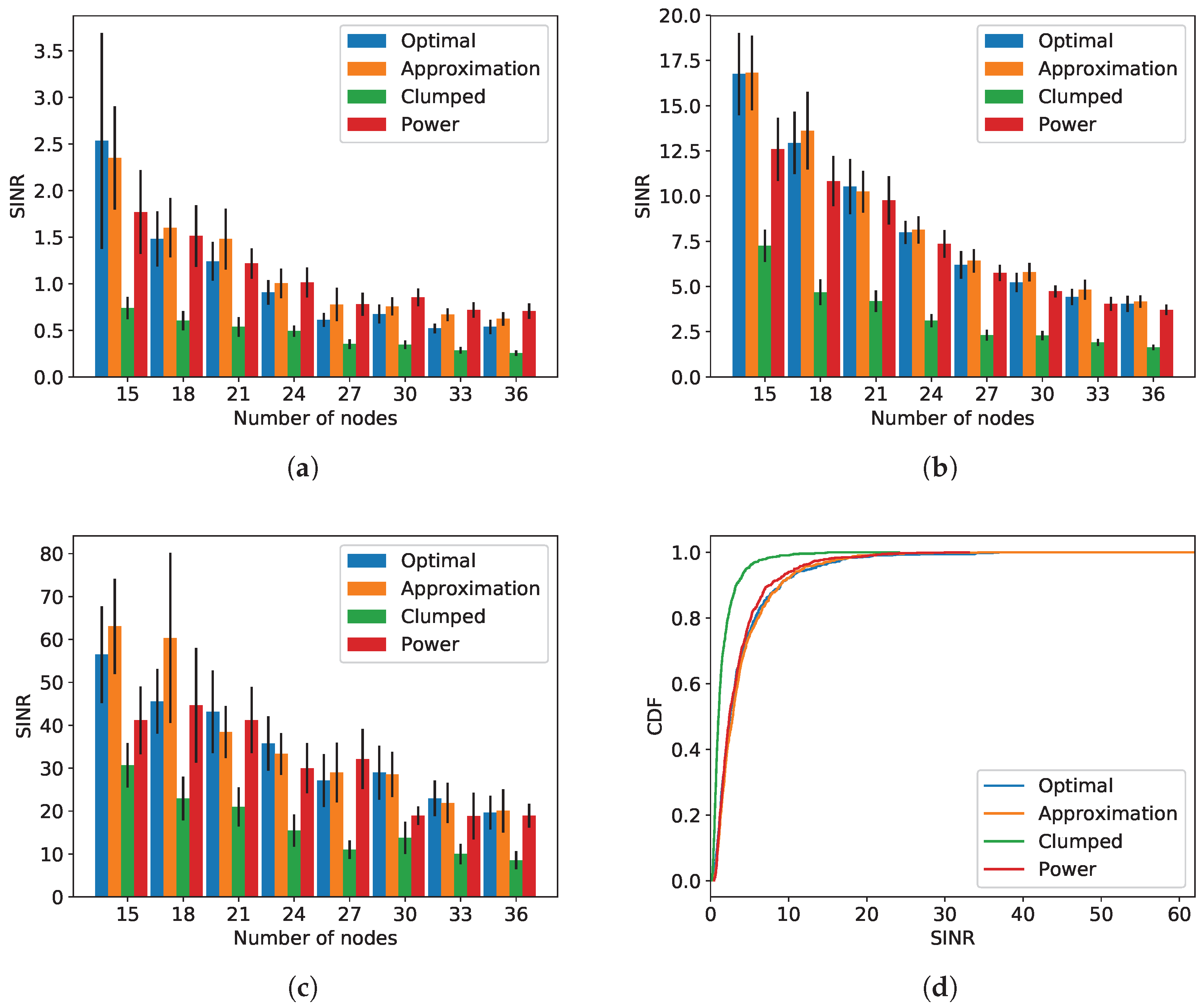
The minimum, average, and maximum SINRs obtained for each algorithm and number of nodes are shown in Figure 4a–c, and Figure 4d shows the CDFs of the SINRs obtained with each algorithm, over all nodes, in network instances with 36 nodes. In the aggregate figures, the values shown are the averages across all instances for each number of nodes, with 95% confidence intervals. As expected, clumped partitioning performed the worst, with the SINR decreasing as the number of nodes increased. The results even show that a bad grouping of nodes can impact the SINR dramatically, degrading the SINR on average by >5 dB for 15–20 nodes per group in the considered scenarios. This shows the potential poor performance that may occur if a partition is chosen that does not take into account the directional properties of the nodes’ channels. All of the other algorithms substantially outperformed clumped partitioning on all three SINR metrics.

The performance of the other three algorithms was similar. Even though the optimization and approximation algorithm used only the two parameters of dominant direction and angular spectrum spread, they were nonetheless able to match the performance of power partitioning, which used the full channel information for each node. This is promising, especially for IoT scenarios, as it demonstrates that an effective node partition can be achieved even with only limited information about the nodes’ channels. Moreover, the directional properties we have used will be relatively stable over time for static or slow-moving nodes, meaning that the signaling needed to facilitate node partitioning is reduced, as channel information need only be collected from the nodes occasionally. In the best case, each time nodes transmit, the channel information obtained from their collected pilot signals can be used to compute the next node partition, even in cases where nodes transmit only infrequently, as in many sensor networks and monitoring applications.

In many cases, we observed a relatively large variance in the SINRs obtained for all algorithms. This is because, although both our partitioning approaches and power partitioning methods were aimed at reducing inter-node interference, a true optimal partition would require actually computing the instantaneous interference between the nodes. This depends on the correlations between the users’ channels, and while both the directional channel properties (for our approach) and the instantaneous power (for power partitioning) correlate with the inter-node interference, they do not perfectly capture it. The variance is greater when the number of nodes is lower, since with fewer nodes the probability of the nodes being more unevenly distributed across the angular spectrum increases, leading to a higher proportion of unusual cases.

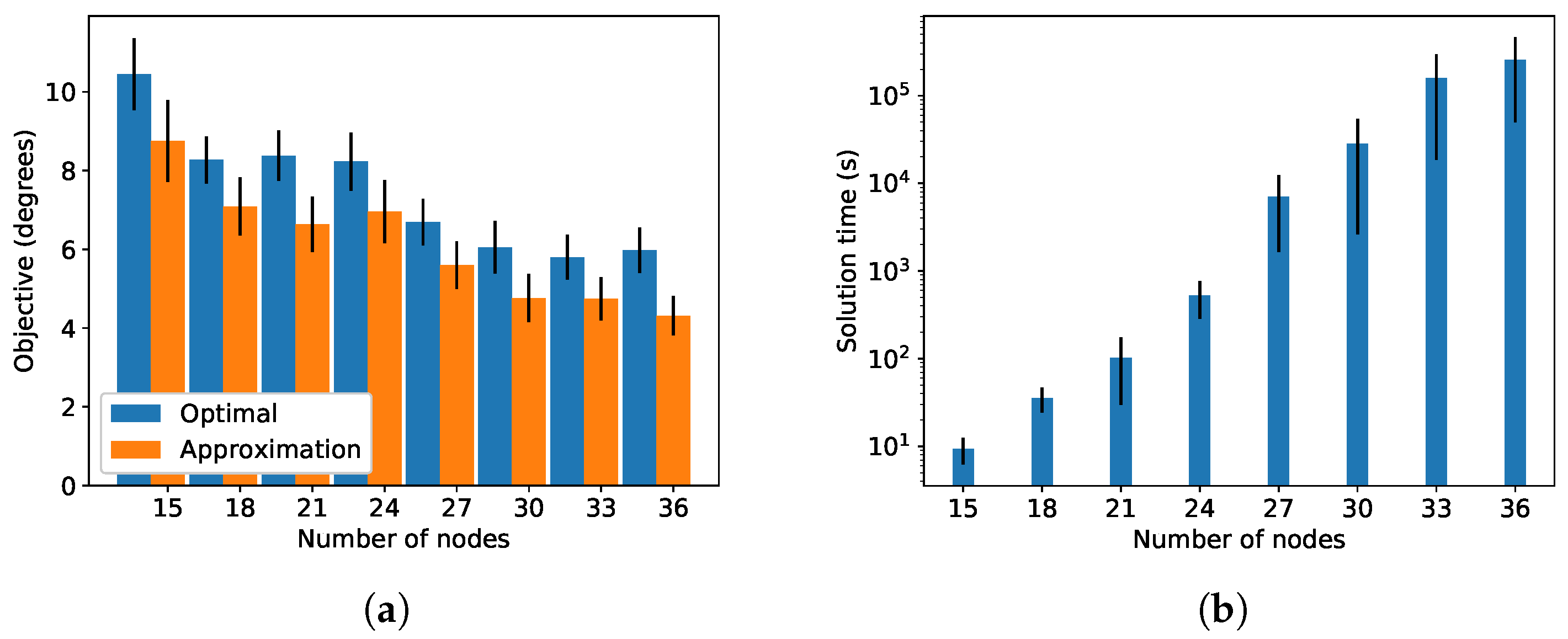
In the figures, we can see that the optimization and approximation algorithms performed similarly, with the approximation algorithm even obtaining a higher SINR in some cases, although the difference between the two was only statistically significant in one case, for the minimum SINR for 33 nodes. The reason that the approximation algorithm was able to achieve better performance than the optimization algorithm is again because here we measured performance in terms of SINR, calculated from the complete node channels, whereas the two algorithms—optimization and approximation—had only reduced channel information available to them in the form of the dominant directions and angular spectrum spreads. In other words, the objective function that the two algorithms were aiming for is not the same as the SINR measures plotted in the figure—only a reasonable proxy for it with reduced channel information. As can be seen in Figure 5a, in terms of the objective function value obtained, the optimization algorithm always outperformed the approximation algorithm, as expected. Across all the cases tested, the approximation algorithm achieved an average of 81% of the optimal objective function value.

Figure 5b shows the time required to solve MMAD to optimality versus the number of nodes. As is typical for this kind of combinatorial optimization problem, the solution time grows exponentially with the problem instance size (note that the solution times are shown on a log scale). For small instances of 15 nodes, the optimization takes less than ten seconds to run, which is feasible in practice for IoT scenarios where nodes transmit on the order of minutes or higher. However, for larger instances, it would not be feasible to use the optimization algorithm; the largest solution time observed was 1,232,518.65 s—more than 14 days—and realistic IoT scenarios can have a far greater number of nodes than we tested here. As a comparison, our Python implementation of the approximation algorithm ran in less than $0.1$ ms for all cases tested. The other comparison algorithms had similarly fast solution times as well. For practical deployments, the approximation algorithm is thus a more appropriate solution. Based on the SINR characteristics for the grouped nodes, further communication-oriented performance parameters such as outage probability and achievable rate can be derived for state-of-the-art transmission schemes [3].

8. Conclusions and Future Work

In this paper we have developed a new method for node grouping in massive MIMO systems based on directional channel characteristics. The two channel properties we use, dominant direction and angular spectrum spread, are typically stable over large timescales, when compared to the full channel information that should be updated at the rate of the coherence time of the channel. Our approach hence enables the grouping of low-power IoT devices with a minimal signaling overhead, even when the devices’ measurement and transmission periods are long. We provided both a mixed-integer optimization formulation and an efficient approximation algorithm to perform the node grouping. In our numerical evaluation, we demonstrated that our approach provides good performance, in terms of the minimum SINR achieved for any node in any group, comparable to a reference method exploiting the full CSI. Our assessment also highlights that a partitioning method that groups nodes with similar directional properties together can have a particularly detrimental effect on link quality due to the interference generated by MRC precoding.

A light signaling user grouping approach, as we have demonstrated in this paper, is valuable for any situation where the signaling overhead is significant. This will be the case when there is a very large number of nodes, as in IoT scenarios. For the end devices, reducing the signaling overhead also reduces energy usage, which is critical for battery powered IoT devices. Although we have thus far only tested cases with up to 36 nodes, and in real IoT deployments the number of nodes is expected to be much greater, the approximation algorithm we have presented shows good scalability and should thus be suitable even in larger scenarios.

In future work, we aim to close the loop by performing measurements in which we measure nodes’ channels and then apply our solutions and measure the performance of the resulting node groups. We also plan to extend our method to take into account errors in the directional channel information. This will not only make the method more robust in case of measurement errors, but will also cater to mobile nodes, since as a node moves, its directional information changes, thus effectively producing an error compared to the last time this information was measured.

The range of scenarios investigated can also be expanded in future work. By focusing on heuristic methods, larger problem instances can be tested, as well as more frequency bands and different numbers of antennas at the base station. Multi-cell and distributed cell-free systems are also an interesting direction in future, in particular the latter, as cell-free architectures are likely to feature prominently in 6G systems, and this further complicates the node grouping problem, since nodes cannot simply be grouped within each cell.