Norm-Based Binary Search Trees for Speeding Up KNN Big Data Classification


Information Technology College, Mutah University; Karak 61710, Jordan
Computers 2018, 7(4), 54; https://0-doi-org.brum.beds.ac.uk/10.3390/computers7040054
Submission received: 26 September 2018
/
Revised: 11 October 2018
/
Accepted: 19 October 2018
/
Published: 21 October 2018
Abstract
:Due to their large sizes and/or dimensions, the classification of Big Data is a challenging task using traditional machine learning, particularly if it is carried out using the well-known K-nearest neighbors classifier (KNN) classifier, which is a slow and lazy classifier by its nature. In this paper, we propose a new approach to Big Data classification using the KNN classifier, which is based on inserting the training examples into a binary search tree to be used later for speeding up the searching process for test examples. For this purpose, we used two methods to sort the training examples. The first calculates the minimum/maximum scaled norm and rounds it to 0 or 1 for each example. Examples with 0-norms are sorted in the left-child of a node, and those with 1-norms are sorted in the right child of the same node; this process continues recursively until we obtain one example or a small number of examples with the same norm in a leaf node. The second proposed method inserts each example into the binary search tree based on its similarity to the examples of the minimum and maximum Euclidean norms. The experimental results of classifying several machine learning big datasets show that both methods are much faster than most of the state-of-the-art methods compared, with competing accuracy rates obtained by the second method, which shows great potential for further enhancements of both methods to be used in practice.
1. Introduction
In the last decade, information technology has developed quickly in terms of quantity, quality and low cost, providing almost everyone on earth with means of communication and data sharing. The availability of many useful sensors, which are cheaper and easier to use than ever to collect data and information along with the strong desire for information have allowed for the emergence of Big Data [1].
Contemporary hardware and software have become somehow depleted for dealing with such an unusual size of data efficiently. For example, a 3 GB file, which is considered as a relatively small Big Data file, cannot be opened using the common Microsoft Excel® software.
Big Data files contain important information, which needs to be processed and analyzed to obtain vital information, or to train an intelligent system based on a larger coverage of the population. Most well-known machine learning algorithms take an unacceptable amount of time to be trained on such Big Data files; for example, the K-nearest neighbors classifier (KNN) took weeks to classify one dataset (Higgs) using advanced hardware. Therefore, Big Data require big thinking to overcome the data size problem and allow our neat algorithms to work efficiently.
The KNN classifier is a slow classifier by its nature, and a lazy learner as it does not have a small fixed-size training model to be used for testing; it utilizes all the training data to test any example. Given a training set of n examples, in d-dimensional feature-space, the running cost to classify one example is O(nd) time, and since we have the curse of Big Data, where n and/or d are large values, the KNN becomes useless, particularly if it is used for an online application.
The major contribution of this paper includes speeding up the slow KNN classifier, particularly when classifying machine learning Big Data sets. This is achieved by proposing a new approach based on inserting the training examples into a binary search tree (BST). To this end, we used two methods. The first utilizes the scaled norm of each example, while the second inserts each example into the binary search tree based on its similarity to the examples of the minimum and maximum Euclidean norms.
The rest of this paper is organized as follows: Section 2 presents some related methods used for speeding up the KNN classifier; Section 3 describes the proposed methods and the dataset used for the experiments; Section 4 evaluates and compares the proposed methods to other state-of-the-art methods; and Section 5 draws some conclusions, shows the limitations of the proposed methods and gives directions for future research.
2. Related Work
Tremendous efforts have been made to increase the speed of the KNN classifier in general, and recently to push for a robust KNN to Big Data. Thus, we will focus on the most recent achievements dealing with Big Data, such as the work of Reference [2], who proposed a parallel implementation based on mapping the training set examples followed by reducing the number of examples that are related to a test sample. The latter method was called Map-Reduce-KNN (MR-kNN). The reported results were similar to those of an exact KNN but much faster, i.e., about 16–149 times faster than the sequential KNN when tested on one dataset of 1 million examples; the speed of the MR-kNN depends mainly on the number of maps (which was in the range of 16–256) and the K-neighbors used. The mapping phase consumes a considerable amount of time, particularly with large values of K. This work is further improved by Reference [3], where they proposed a new KNN based on Spark (kNN-IS) which is similar to the Mapping/Reducing technique but using multiple reducers to speed up the process; the size of the dataset used went up to 11 million examples.
Based on clustering the training set using a K-means clustering algorithm, Reference [4] proposed two methods to increase the speed of KNN: The first method used random clustering (RC-KNN( while the second used landmark spectral clustering (LC-KNN). When finding the related cluster, both methods utilized the sequential KNN to classify the test example with a smaller set of training examples. Both algorithms were evaluated on nine big datasets showing reasonable approximations to the sequential KNN; the reported accuracy of the results depended on the number of clusters used.
Another clustering approach was utilized recently by Reference [5], who proposed two clustering methods to accelerate the speed of the KNN, called (cKNN) and (cKNN+). Both methods are similar, however the latter uses a cluster augmentation process. The reported average accuracy of all the big datasets used was in the range of 83%–90%, depending on the number of clusters and K-neighbors used. However, these results improved significantly when they used Deep Neural Networks for learning a suitable representation for the classification task.
Two recent and interesting approaches proposed by Reference [6] deal with the problem differently, using random and Principal Component Analysis (PCA) techniques to divide the data to obtain multivariate decision tree classifiers (MDT). Both methods (MDT1 and MDT2) were evaluated on several big datasets, and the reported performance of the MDT2 was relatively better than that of the MDT1, considering all the datasets used, showing that data partitioning using PCA is better than that of the random technique in terms of accuracy.
Most of the proposed work in this domain is based on the divide and conquer approach; this is a logical approach to use with big datasets, and therefore, most of these approaches are based on clustering, splitting, or partitioning the data to turn and reduce their huge size to a manageable one that can be targeted later by KNN. One major problem associated with such approaches is the determination of the best number of clusters/parts, since more clusters means fewer data for each cluster, and therefore faster testing. However, fewer data for each cluster means less accuracy, as the examples hosted by the cluster found might not be related to the tested example. On the contrary, few clusters indicate a large number of examples for each, which increases the accuracy but slows down the classification process. We can call this phenomenon the clusters-accuracy-time dilemma.
Another related problem is finding the best k for the KNN, which is beyond the scope of this paper; for more on this, see Reference [7,8]. In this work, we will work on k = 1, i.e., the nearest neighbor.
Regardless of the high quality and quantity of the proposed methods in this domain, there is still room for improvement in terms of accuracy and time consumed for both the training and the testing stages.
In this paper, we avoid the clustering approach by proposing a new approach based on inserting the training examples into a binary search tree, using the scaled norm of each example, or the minimum and maximum Euclidean norms. The use of tree data structures to speed up the KNN classifiers is not new, since there is extensive literature on tree structures such as Furthest-Pair-Based Binary Search Tree [9], k-d trees [10], metric trees [11], cover trees [12], and other related work such as Reference [13,14]. Our work is similar to these approaches in that it exploits a tree structure to speed up the search process. However, our proposed methods are distinguished from the other approaches by their simplicity, interpretability, ease of implementation, and high ability to process Big data.
3. Norm-Based Binary Search Trees
In this paper, we propose the use of the Euclidian norm as a signature for each feature vector, to then be used by a binary search tree, which stores examples of the same norms based on their similarity. The first method, which we call the norm-based binary tree (NBT), uses only norm information when developing the binary tree, while the second one, which is an enhancement of the first, stores the examples based on their similarity to the feature vector of the minimum norm and the feature vector of the maximum norm; we call the latter method the Minimum/Maximum norms-based binary tree (MNBT). The test phases of both methods use the same approaches to search their binary tree (BT) to the leaf, and then the sequential KNN classifier is employed to classify the feature vectors found in the searched leaf.
3.1. NBT
Given a training dataset with n feature vectors (FV) and d features, the NBT builds its binary search tree by calculating the Euclidean norms (EN) for each FV and stores their indexes in the root of a binary tree; the ENs are scaled to the range [0, 1] and then rounded to {0, 1}. The indexes of FVs with EN rounded to (0) are stored in the left-child node, while those with the EN rounded to (1) are stored in the right child. The NBT continues calculating and clustering the FVs recursively until it obtains only one FV in a leaf node, or a number of FVs with the same EN. It is worth noting that for FVs that are clustered to either 0 or 1, in the next iteration their scaled EN might be the opposite, and this is why the NBT continues clustering recursively until it reaches a leaf-node hosting one FV or some FVs with similar norms, i.e., this method assumes that each FV has a unique norm, or at least, the number of FVs that share the same norm is relatively small. Algorithm 1 describes building the binary search tree for the NBT. The time complexity of building the binary tree is O(n d + n log n), however if n >> d it can be approximated to O(n log n). Obviously, the d extra running cost comes from calculating the Euclidian.
In the test phase, the NBT calculates the EN for each test FV, then scales and rounds these ENs in the same way as in the training phase, and recursively searches the tree to the leaf to find one or more FVs, which will be fed to the sequential KNN algorithm. Searching the tree costs O(log n) time for each test example in all cases, and therefore the KNN time complexity becomes O(d) for each tested FV if and only if there was only one FV in the leaf node found, which is very fast. However, when there is m FVs in the leaf found, the time complexity grows depending on the size of m. In the worst case, where all the FVs are of the same EN, the overall time complexity becomes even more than that of the sequential KNN, which is O(nd) time, in addition to the time consumed by the searching process for each test example. Algorithm 2 shows the test phase of the NBT. We evaluated both methods using several machine learning big datasets, and compared their performances with those of the aforementioned state-of-the-art methods.
| Algorithm 1: Training Phase of the NBT. |
| Input: Numerical training dataset DATA with n FVs and d features. Output: A Root pointer of the NBT Binary search tree. for each point FVi in DATA, do Array ENorm [i] ← EN(FVi) Array ExampleIndexes [i] ← i End Create Tree Root Node RootN RootN.Min ←Minimum (ENorm) RootN.Max ←Maximum (ENorm) RootN.Enorm ← ENorm RootN.Left = Null RootN.Right = Null Procedure BuildTree (Node ← RootN) for each FVi in Node, do Scale ← (Node.Enorm[i]-Node.Min)/( Node.Max- Node.Min) Scale ← round(Scale) if (scale = 0) Add index of FVi to Node.Left.Enorm else Add index of FVi to Node.Right.Enorm end if (Node.Left = Null or Node.Right = Null) return end Node.Left.Max ← Maximum (Node.Left.ENorm) Node.Left.Min ← Minimum (Node.Left.ENorm) Node.Right.Max ← Maximum (Node.Right.ENorm) Node.Right.Min ← Minimum (Node.Right.ENorm) BuildTree (Node.Left) BuildTree (Node.Right) end Procedure return RootN |
| Algorithm 2: Testing Phase of the NBT. |
| Input: Numerical testing dataset TESTDATA with n FVs and d features. Output: Test Accuracy. Accuracy ← 0 for each FVi in TESTDATA, do ENorm ← EN(FVi) Procedure GetNode (Node ← RootN, Enorm) Scale ← (Node.Enorm[i]-Node.Min)/(Node.Max-Node.Min) Scale ← round (Scale) if (Scale = 0 and Node.Left) return GetNode(Node.Left, Enorm) else if (Scale = 1 and Node.Right) return GetNode(Node.Right, Enorm) else return Node end end Procedure Procedure KNN (FVi, Node) Array Distances; for each fvj in Node, do Distances[j] ← EuclideanDistance [fvj, FVi] end index ← argmin (Distances[j]) return c ← Class (fvindex) end Procedure if c = Class (FVi) Accuracy ← Accuracy+1 end end Accuracy ← Accuracy/n return Accuracy |
3.2. MNBT
Similarly to the NBT, this method trains a binary search tree where each node stores a number of training examples based on their similarity to two FVs stored in the parent node: the first FV is the one with the minimum EN (FV1), and the other FV (FV2) is the one with the maximum EN from the training data. To build the Binary search tree, the MNBT uses the Euclidian distance to find similar FVs to the FV1, and stores them in the left node, and those similar to the FV2 are stored in the right node of a parent node with the FV1 and FV2. Recursively, the MNBT continues to cluster all the FVs of the training data in a binary search tree, until they become one point, which is stored in a leaf node. However, if the minimum EN is equal to the Maximum EN, then all the FVs remain in the parent node, which becomes a leaf node, as they cannot be further clustered.
Ideally, building the tree using the MNBT takes O(n.d + n.d log n) time: the first (n.d) time is consumed by the process of finding the ENs for each FV in the training data, and the second (n.d) time is consumed by the similarity process, which uses the Euclidian distance along all the features (d). Obviously this takes more time than the NBT because of the extra calculations, but we expect it to perform better in terms of classification accuracy, as clustering is carried out based on the similarity to the actual FVs rather than the EN information, which is sometimes misleading.
The testing stage is also similar to that of the NBT; given the trained binary search tree and a test fv, the MNBT searches for this fv starting from the root node, comparing its similarity to the stored FV1 and FV2 in each node, and then it finds its way left or right recursively, until it finds the leaf node. This node is then inputted to the KNN with the test fv to predict the class of the test example.
Searching the MNBT tree costs O(2d log n) in all cases, which is relatively fast, but slower than that of the NBT, particularly when d is very large, i.e., >1000; the extra (2d) time comes from the comparison of the tested FV with the stored FV1 and FV2.
The worst-case scenario of the MNBT is similar to that of the NBT; principally, when the EN of all the FVs is the same, then FV1 is more likely to be equal to FV2, which results in hosting all the FVs or at least a large number of them in one leaf node, and the MNBT overall classification time then ends with O(2d log n + n.d) time. Table 1 summarizes the time complexity for both of the proposed methods.
Building the tree of the MNBT can be described using Algorithm 1 if we replace the Minimum norm (Node. Min) with the index of FV1, and the Maximum norm (Node. Max) with FV2, in addition to replacing the lines of scaling and comparing (to 0 and 1) with calculating and comparing the similarity of the tested FV with both FV1 and FV2. The same alteration applies to Algorithm 2 to comply with the MNBT method.
3.3. Implementation Example
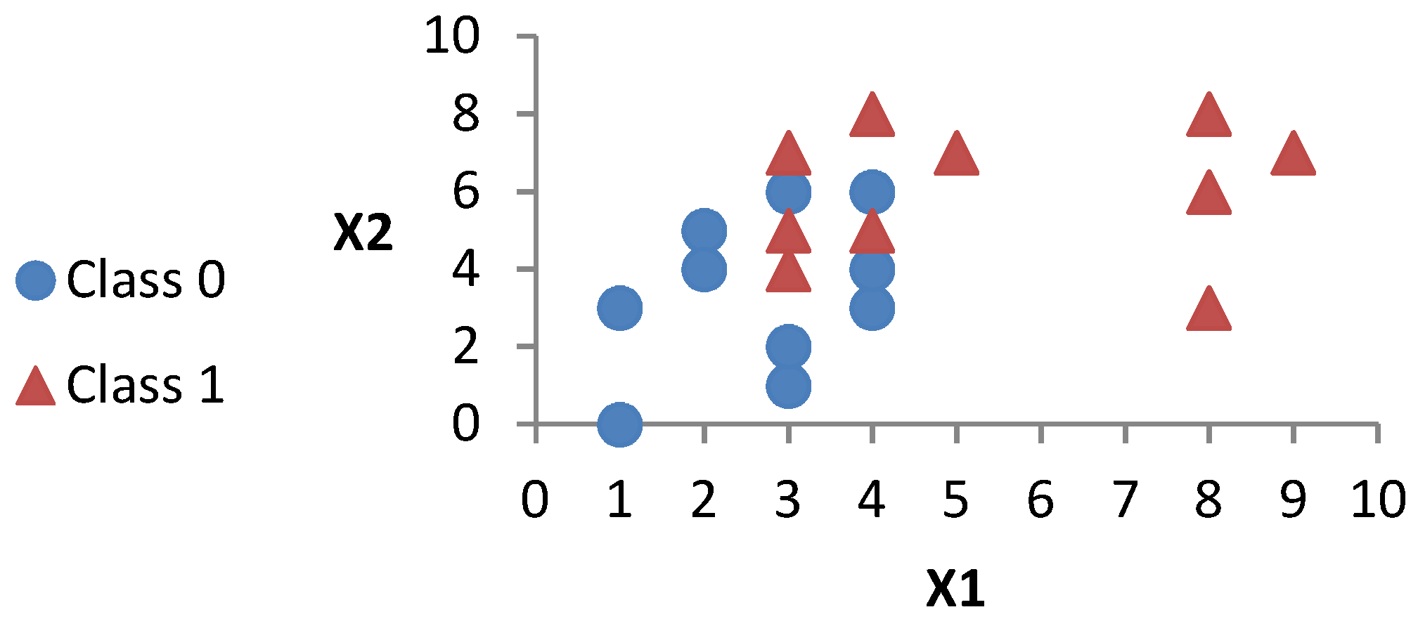
In this section, we implement the proposed methods to create two binary search trees: the first uses the NBT and the second uses the MNBT. To this end, we used small synthesized data for illustration purposes. The synthesized dataset used consists of two hypothetical features (X1 and X2) and two classes (0 and 1) with 20 examples, as shown in Table 2 and illustrated in Figure 1.
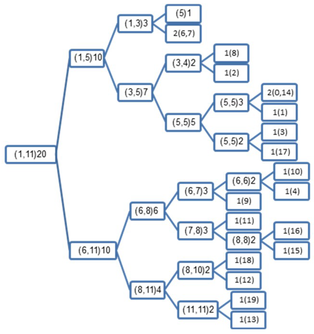
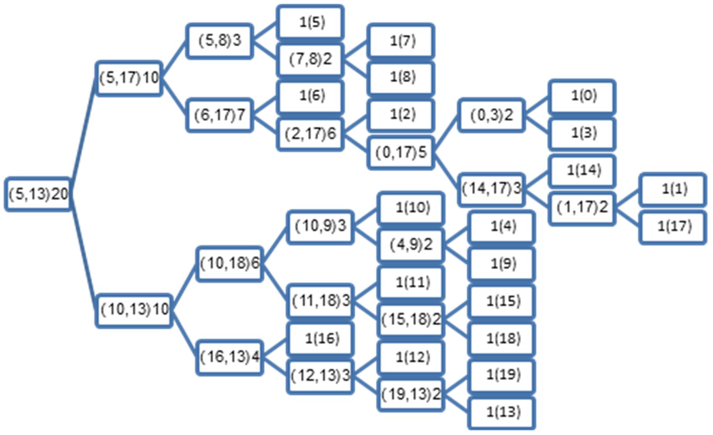
If we apply the NBT to the synthesized dataset we get the BT illustrated in Figure 2, and when applying the MNBT to the same dataset we get the BT illustrated in Figure 3.
It is noteworthy that the norms shown in the BT inside the brackets in Figure 2 are the integers of the minimum and maximum norms; we used this integer format to make the size of the BT compact. Both Figure 2 and Figure 3 summarize the proposed methods. For example, the root node in Figure 2 shows that the minimum norm of all examples is 1 and the maximum norm is 11.3. It is important to keep track of these values to be used in the test phase, as they are essential to scale the test norm to 0 or 1, so that the algorithm will be able to direct the search process; if the scaled norm is 0 it goes to the left node, otherwise it goes to the right node, until it reaches a leaf node. At the end, the KNN is applied to the hosted examples there.
It is interesting to note the second leaf node in Figure 2 {2(6,7)}: despite being a leaf node, it hosts two examples (6 and 7), as can be seen from Table 2. Both examples share the same norm (3.2), and are therefore stored together in a leaf node. Having a large number of examples that share the same norm is problematic for the NBT, as these examples might be completely different, and the test example will be directed to use these examples with the KNN, which might yield undesired results. The same remark applies to examples (0, and 14) sharing the same norm (5). However, this is not always the case, as there are many leaf nodes in both Figures with only one example, which makes the testing phase very fast for both of the proposed methods.
In terms of classification accuracy, if we have a dataset with a limited number of similar norms (like the one in Table 2), we can see that from the first split of the resultant BST, all of the similar examples with relatively small norms are stored to the left of the BST, namely, {0, 1, 2, 3, 5, 6, 7, 8, 14, 17}, see the upper side of Figure 2, and all of the similar examples with relatively large norms are stored to the right of the BST, namely, {4, 9, 10, 11, 12, 13, 15, 16, 18, 19}, see the lower side of Figure 2. Ideally, if we have a perfect sorting of the training examples (i.e., training examples from the same class are stored together) the classification accuracy should be improved.
It is also interesting to note that some examples from class 0 are sorted unexpectedly on the right side, and some examples from class 1 are sorted unexpectedly on the left side. This is due to the large and small norms of both examples, where they should have small and large norms to match other examples from their own classes. However, this should not be problematic, as each example has its own class, and at the end of the process we use the KNN to decide the new class of the test example regardless of the place inside the created BT.
On the other hand, the MNBT illustrated in Figure 3 stores the indexes of the examples with the minimum and maximum norms, as seen in the root node, where these examples are 5 and 13. The first example (5) has the minimum norm 1, and the second example (13) has the maximum norm 11.4. These examples (5 and 13) will be used in the test phase of the MNBT by measuring their similarities to a test example; if it is similar to example 5, the search process is directed to the left node, and otherwise it is directed to the right node. The same process is executed at each point, exploiting the stored indexes; the search process is directed left/right until it reaches a leaf node, and only then is the KNN applied to the hosted examples found in that particular leaf node.
It is interesting to note from Figure 3 that the starting examples (5 and 13) were used effectively to sort the rest of the examples (including their own) in the created BT, in a way that facilitates future searches; as we can see from the first split, most of the similar examples from class 0 are stored to the left {0, 1, 2, 3, 5, 6, 7, 8}, with exceptions {4, 9}. And most of the similar examples from class 1 are stored to the right {10, 11, 12, 13, 15, 16, 18, 19}, with exceptions {14, 17}, as can be seen from Figure 3. However, this should not make a big difference in the test phase, as each example has its own class, and at the end of the process we use the KNN to decide the new class of the test example regardless of the place inside the created BT.
3.4. Data
To evaluate and compare our methods, we used well-known machine learning datasets, which were obtained from the Machine Learning Repository [15] and the support vector machine library datasets (LIBSVM) [16]. These datasets are normally used for evaluating machine learning methods, and are therefore reused here for comparison purposes. We used intermediate and large numerical datasets, with different dimensions and sizes. The numerical data include Boolean (B), Integers (I), negative (N), and Real numbers (R). Table 3 shows the description of the datasets used.
4. Results and Discussions
We conducted several experiments to evaluate the proposed methods after programming both NBT and MNBT using C++ to classify the datasets described in Table 3. To make a valid comparison with other methods, and since different researchers used different evaluation schemes and different datasets, each of our experiments followed the experimental settings of the compared method. The hardware used was the Azure high-performance computing virtual machine with 16 Intel® CPUs @ 2.3 GHz with 32 GB RAM, and no computer cluster was used. However, the proposed algorithms had not benefited from the Multi CPUs available, because they were single-threaded, and the machine used could not run a single thread on multiple CPUs simultaneously. However, this allowed for more experiments to run at the same time, as each experiment ran on a dedicated single CPU. Since each of the previous methods used different hardware with a different computation power, we opted to measure the speed-up of the algorithm similarly to [2] by comparing the time consumed with that of the sequential KNN algorithm on the same machine as follows:
where “reference time” is the runtime consumed by the sequential KNN, and “algorithm time” is the runtime consumed by other algorithms that we want to compute their speed-up factor.
To compare our results with the MR-KNN and KNN-IS, we evaluated our methods on the same datasets used, namely Poker and Susy, with the same 5-fold cross-validation (CV); the results are shown in Table 4 and Table 5.
The accuracy results recorded in Table 4 look the same for both methods of MR-KNN and KNN-IS, because these algorithms are parallel-exact algorithms. Despite being approximate, the proposed MNBT outperformed both methods compared in terms of accuracy and speed on both datasets, as can be seen from Table 4 and Table 5, where the MNBT is found to be much faster than both MR-KNN and KNN-IS, and more accurate as well. With reasonable results, we also can see that the proposed NBT is much faster than all the methods mentioned in Table 5; the reason for this significant high speed is the use of the norm without the need for using the Euclidian distance (ED) (which relies on the dimensions of the dataset) as in the MNBT.
To compare our results with the RC-KNN and LC-KNN methods we evaluated our methods on the same datasets used, with the same 10-fold-CV, as shown in Table 6 and Table 7.
As can be seen from Table 5 and Table 6, the accuracy achieved by the proposed NBT was very low for these datasets; this is due to the nature of the data contained in these datasets, which either contain negative and positive numbers, or a large number of zeros. Both situations yield a similar EN for different examples, and therefore, the NBT inserts these examples in the wrong locations in the binary search tree. However, its speed-ups are much higher than those of all methods, as expected, while the MNBT outperforms the RC-KNN with competing results compared to the LC-KNN, with much higher speed-ups.
To compare our results with the cKNN and cKNN+, we evaluated our methods on the same datasets used, with the same 5-fold-CV, as shown in Table 8. It is worth mentioning that there was no reported consumed time for both the cKNN and the cKNN+, instead Reference [5] reported the number of distances used, and the authors also reported the average accuracy on all the datasets used, which was almost the same for both the cKNN and the cKNN+ in the range of 83%–90% depending on the number of clusters and neighbors (K) used.
Again, we can see the poor performance of our norm-based method (NBT) particularly on the Nist dataset, where the dataset contains many repetitions of 0s and 255s, while the MNBT performs much better than the NBT and, in some datasets, outperforms the maximum average accuracy of both cKNN and cKNN+.
To compare our results with the MDT1 and MDT2, we evaluated our methods on the same available datasets used, with the same test ratios used, which was in the range of 19–97% depending on the dataset used, as shown in Table 9 and Table 10.
As can be noted from Table 10, the time consumed by the proposed methods was very short compared to that of the pure 1NN (our implementation in the last column). For example, the NBT took about 5.75 minutes, and the MNBT took about 20 minutes on the Higgs dataset, while our implantation of the 1NN took more than 6 weeks on the same datasets. It is noteworthy that the time consumed by the MDT1 and MDT2 cannot be compared to the time consumed by the proposed methods because both algorithms were tested on a different machine, which is why we used the speed-up factor shown in Table 11, which is generated from Table 10 using Equation (1) for this experiment.
It is interesting to note from Table 9 and Table 11 (row 8) that the accuracies of both of the NBT and the MNBT are the same as the KNN (with k = 1); this is because of the nature of the data contained in the Connect4 datasets, since the Connect4 data is nothing but a combination of (x, o and b), which are replaced by (1, 2, 3), respectively, to comply with the KNN as being a numeric classifier. Furthermore, the speed-up of both of the proposed algorithms is 1, meaning that they consume almost the same time as the KNN; the reason for that is the similar norms of all the examples, which makes it possible to insert all the examples in one leaf node in the binary search tree. However, we can observe a good performance in terms of accuracy achieved by the MNBT, which outperforms the MDT1 in most datasets, and rivals the MDT2 results. We could not calculate the speed-up of both Susy and Higgs in this experiment because they both consume an unacceptable amount of time.
In summary, the previous presentation and discussion of the proposed NBT and MNBT results show that these methods are very fast compared to other methods when classifying Big Data using the KNN approach, with expected humble accuracy rates of the NBT, and relatively significant enhanced accuracy rates of the MNBT, which means it is possible to build on these methods to further enhance the accuracy rates exploiting the speed characteristics of both. As can be seen from the previous results, most are data-dependent, i.e., the proposed method perform well with some datasets and poorly with others. This is because both of the proposed methods depend on the norm of the FVs, particularly the NBT, which is more dependent on the norm. The data contained in these datasets are of different nature, i.e. some of them contain negative and positive numbers, or a large number of zeros, in such situations, calculating the EN yields similar norms for different examples belonging to different classes. Therefore, the building algorithms of the proposed MNBT and NBT sorts these examples in wrong locations within their binary search trees, which makes finding the nearest ones to a test example a difficult task for the search algorithms; and this is the major limitation of both the proposed algorithms.
5. Conclusions
In this paper, we proposed a new approach based on inserting training examples into a binary search tree. We used two methods: The first utilizes the scaled norm of each example and called the NBT, the second is based on inserting each example depending on its similarity to the examples of the minimum and maximum norms and called the MNBT. The experimental results on different intermediate and big datasets show the high classification speed of both methods; however, the results were data-dependent, particularly when using the NBT, i.e., the greater the uniqueness of the EN of the data examples, the higher the accuracy results will be. However, if this constraint is extremely violated, poor results are to be expected from both methods, particularly the NBT, which is more dependent on the EN calculation. Ideally, this constraint is violated when we have data with negative and positive numbers, permutations of some numbers, and many zeros or permutations of the same number, as all these situations yield similar norms from different examples. This is to be expected from the beginning; however, the reason for proposing the NBT is its outstanding speed (log n) compared to all the methods evaluated. This strong characteristic can be used to hybridize and further enhance the proposed methods to obtain fast and more accurate algorithms, which is what we have done when we proposed the MNBT, which is much faster than most of the algorithms compared, with competing accuracy.
It is possible to increase the accuracy of the proposed methods by considering more points from the higher levels of the binary search tree, and not only those found in a leaf-node, but this will also increase the number of examples that are fed to the KNN classifier. Consequently, this will increase the running cost. However, since both the proposed algorithms are extremely fast compared to other methods, we may not worry much about the running cost, particularly if the number of examples increased is controlled to a specific value, say log n for instance. Such a modification will be left for future work, along with other enhancements such as using random points if the minimum and maximum norms are equal, in addition to trying other norms and distance metrics such as the Hassanat distance [17,18] to address the major limitation (accuracy) of the proposed methods. It is also possible to increase the accuracy of the classification using different methods to store data points in the BST, such as the furthest-pair of points [19]; such a method might increase the accuracy but this would be at the expense of the classification speed, as shown in Reference [9].
Supplementary Materials
The datasets used in this paper are available online: http://archive.ics.uci.edu/ml and https://www.csie.ntu.edu.tw/~cjlin/libsvmtools/datasets.
Funding
This research received no external funding.
Conflicts of Interest
The author declares no conflict of interest.
References
- Bolón-Canedo, V.; Remeseiro, B.; Sechidis, K.; Martinez-Rego, D.; Alonso-Betanzos, A. Algorithmic challenges in Big Data analytics. In Proceedings of the European Symposium on Artificial Neural Networks, Computational Intelligence and Machine Learning, Bruges, Belgium, 26–28 April 2017; pp. 517–529. [Google Scholar]
- Maillo, J.; Triguero, I.; Herrera, F. A mapreduce-based k-nearest neighbor approach for big data classification. In Proceedings of the 2015 IEEE Trustcom/BigDataSE/ISPA, Helsinki, Finland, 20–22 August 2015. [Google Scholar]
- Maillo, J.; Ramírez, S.; Triguero, I.; Herrera, F. kNN-IS: An Iterative Spark-based design of the k-Nearest Neighbors classifier for big data. Knowl.-Based Syst. 2017, 117, 3–15. [Google Scholar] [CrossRef] [Green Version]
- Deng, Z.; Zhu, X.; Cheng, D.; Zong, M.; Zhang, S. Efficient kNN classification algorithm for big data. Neurocomputing 2016, 195, 143–148. [Google Scholar] [CrossRef]
- Gallego, A.J.; Calvo-Zaragoza, J.; Valero-Mas, J.J.; Rico-Juan, J.R. Clustering-based k-nearest neighbor classification for large-scale data with neural codes representation. Pattern Recognit. 2018, 74, 531–543. [Google Scholar] [CrossRef]
- Wang, F.; Wang, Q.; Nie, F.; Yu, W.; Wang, R. Efficient tree classifiers for large scale datasets. Neurocomputing 2018, 284, 70–79. [Google Scholar] [CrossRef]
- Zhang, S.; Li, X.; Zong, M.; Zhu, X.; Wang, R. Efficient knn classification with different numbers of nearest neighbors. IEEE Trans. Neural Netw. Learn. Syst. 2018, 29, 1774–1785. [Google Scholar] [CrossRef] [PubMed]
- Hassanat, A.B.; Abbadi, M.A.; Altarawneh, G.A.; Alhasanat, A.A. Solving the problem of the K parameter in the KNN classifier using an ensemble learning approach. arXiv, 2014; arXiv:1409.0919. [Google Scholar]
- Hassanat, A.B. Furthest-pair-based binary search tree for speeding big data classification using k-nearest neighbors. Big Data 2018, 6, 225–235. [Google Scholar] [CrossRef]
- Bentley, J.L. Multidimensional binary search trees used for associative searching. Commun. ACM 1975, 18, 509–517. [Google Scholar] [CrossRef]
- Uhlmann, J.K. Satisfying general proximity/similarity queries with metric trees. Inf. Process. Lett. 1991, 40, 175–179. [Google Scholar] [CrossRef]
- Beygelzimer, A.; Kakade, S.; Langford, J. Cover trees for nearest neighbor. In Proceedings of the 23rd International Conference on Machine Learning, Pittsburgh, PA, USA, 25–29 June 2006. [Google Scholar]
- Kibriya, A.M.; Frank, E. An empirical comparison of exact nearest neighbour algorithms. In Proceedings of the 11th European Conference on Principles and Practice of Knowledge Discovery in Databases, Warsaw, Poland, 17–21 September 2007. [Google Scholar]
- Cislak, A.; Grabowski, S. Experimental evaluation of selected tree structures for exact and approximate k-nearest neighbor classification. In Proceedings of the Federated Conference on Computer Science and Information Systems (FedCSIS), Warsaw, Poland, 7–10 September 2014. [Google Scholar]
- Welcome to the UC Irvine Machine Learning Repository. Available online: http://archive.ics.uci.edu/ml (accessed on 11 March 2018).
- Fan, R.E. LIBSVM Data: Classification, Regression, and Multi-Label. Available online: https://www.csie.ntu.edu.tw/~cjlin/libsvmtools/datasets/ (accessed on 12 March 2018).
- Hassanat, A.B.A. Dimensionality invariant similarity measure. J. Am. Sci. 2014, 10, 221–226. [Google Scholar]
- Alkasassbeh, M.; Altarawneh, G.A.; Hassanat, A. On enhancing the performance of nearest neighbour classifiers using hassanat distance metric. Can. J. Pure Appl. Sci. 2015, 9, 3291–3298. [Google Scholar]
- Hassanat, A.B. Greedy algorithms for approximating the diameter of machine learning datasets in multidimensional euclidean space: Experimental results. Adv. Distrib. Comput. Artif. Intell. J. 2018, 7, 1–12. [Google Scholar]
Figure 1.
Illustration of the synthesized dataset from Table 2.
Figure 1.
Illustration of the synthesized dataset from Table 2.

Figure 2.
Illustration of the binary search tree (BST), which is created by the norm-based binary tree (NBT) using the synthesized dataset from Table 2: the number outside the brackets indicates the number of examples hosted by each node, and those inside the brackets indicate the index(es) of the example(s) in a leaf node, or the integers of the minimum and maximum norms of the hosted examples.

Figure 3.
Illustration of the binary search tree (BST), which is created by the Minimum/Maximum norms-based binary tree (MNBT) using the synthesized dataset from Table 2: the number outside the brackets indicates the number of examples hosted by each node, and those inside the brackets indicate the index(es) of the example(s) in a leaf node, or the indexes of the examples of the minimum and maximum norms of the hosted examples.


Table 1.
Summary of time complexity.
| NBT | MNBT | |
|---|---|---|
| Building time complexity | O(n.d + n log n) | O(n.d + n.d log n) |
| search time complexity | O(log n) | O(2d log n) |
| Testing time complexity (search time + KNN time) | O(m.d + log n) * and in the worst case: O(n.d + log n) | O(2d log n + m.d) and in the worst case: O(2d log n + n.d) |
* where m is the number of examples found in a leaf node.
Table 2.
A small synthesized dataset for illustration purposes.
| #Example | X1 | X2 | Class | Euclidean Norms |
|---|---|---|---|---|
| 0 | 4 | 3 | 0 | 5.0 |
| 1 | 2 | 5 | 0 | 5.4 |
| 2 | 2 | 4 | 0 | 4.5 |
| 3 | 4 | 4 | 0 | 5.7 |
| 4 | 3 | 6 | 0 | 6.7 |
| 5 | 1 | 0 | 0 | 1.0 |
| 6 | 1 | 3 | 0 | 3.2 |
| 7 | 3 | 1 | 0 | 3.2 |
| 8 | 3 | 2 | 0 | 3.6 |
| 9 | 4 | 6 | 0 | 7.2 |
| 10 | 4 | 5 | 1 | 6.4 |
| 11 | 3 | 7 | 1 | 7.6 |
| 12 | 8 | 6 | 1 | 10.0 |
| 13 | 9 | 7 | 1 | 11.4 |
| 14 | 3 | 4 | 1 | 5.0 |
| 15 | 5 | 7 | 1 | 8.6 |
| 16 | 8 | 3 | 1 | 8.5 |
| 17 | 3 | 5 | 1 | 5.8 |
| 18 | 4 | 8 | 1 | 8.9 |
| 19 | 8 | 8 | 1 | 11.3 |
Table 3.
Datasets used and their description.
| Dataset | Size | Dimensions | Type |
|---|---|---|---|
| Homus | 15199 | 1600 | I |
| Nist | 44951 | 1024 | I |
| Satimage | 6435 | 36 | R |
| Usps | 9298 | 256 | R |
| Pendigits | 10,992 | 16 | I |
| Gisette | 13,500 | 5000 | I |
| Letter | 20,000 | 16 | R |
| Connect4 | 67,557 | 42 | I |
| Mnist | 70,000 | 784 | I |
| Covtype | 581,012 | 54 | I |
| Poker | 1,025,010 | 11 | I |
| Susy | 5,000,000 | 18 | R |
| Higgs | 11,000,000 | 28 | R |
Table 4.
Classification accuracy comparison of MR-KNN and KNN-IS, with 5-fold-CV.
| Method | Dataset | Accuracy | AvgRunTime (ms) |
|---|---|---|---|
| MR-KNN | Poker | 0.502 | 804,456 |
| Susy | 0.694 | 12,367,966 | |
| KNN-IS | Poker | 0.502 | 102,938 |
| Susy | 0.694 | 1,900,039 | |
| NBT | Poker | 0.519 | 296,639 |
| Susy | 0.594 | 68,227 | |
| MNBT | Poker | 0.530 | 43,345 |
| Susy | 0.710 | 395,464 | |
| KNN | Poker | 0.502 | 105,475,006 |
| Susy | 0.694 | 3,258,848,811 |
Table 5.
Speed-up comparison of MR-KNN and KNN-IS, with 5-fold-CV.
| Method | Poker | Susy |
|---|---|---|
| MR-KNN | 131 | 263 |
| KNN-IS | 1025 | 1715 |
| NBT | 356 | 47,765 |
| MNBT | 2433 | 8241 |
Table 6.
Classification accuracy comparison of RC-KNN and LC-KNN, with 10-fold-CV.
| Dataset | RC-KNN | LC-KNN | KNN | NBT | MNBT | Our KNN |
|---|---|---|---|---|---|---|
| Usps | 0.903 | 0.936 | 0.95 | 0.336 | 0.864 | 0.97 |
| Mnist | 0.722 | 0.839 | 0.86 | 0.190 | 0.858 | 0.97 |
| Gisette | 0.931 | 0.953 | 0.97 | 0.616 | 0.884 | 0.96 |
| Letter | 0.789 | 0.950 | 0.95 | 0.327 | 0.802 | 0.96 |
| Pendigits | 0.945 | 0.972 | 0.98 | 0.254 | 0.966 | 0.99 |
| Satimage | 0.860 | 0.888 | 0.91 | 0.400 | 0.875 | 0.90 |
| Average | 0.858 | 0.923 | 0.936 | 0.354 | 0.875 | 0.961 |
Table 7.
Speed-up comparison of RC-KNN and LC-KNN, with 10-fold-CV.
| Dataset | RC-KNN | LC-KNN | NBT | MNBT |
|---|---|---|---|---|
| Usps | 9.2 | 8.7 | 1035 | 203 |
| Mnist | 8.2 | 6.8 | 9130 | 368 |
| Gisette | 9.3 | 7.6 | 2479 | 68 |
| Letter | 6.1 | 6.0 | 111 | 91 |
| Pendigits | 3.1 | 3.0 | 79 | 55 |
| Satimage | 2.8 | 2.7 | 64 | 35 |
Table 8.
Classification accuracy comparison of NBT and MNBT, with 5-fold-CV.
| Database | NBT | MNBT | KNN |
|---|---|---|---|
| Gisette | 0.609 | 0.888 | 0.960 |
| Letter | 0.313 | 0.799 | 0.957 |
| Homus | 0.120 | 0.555 | 0.647 |
| Satimage | 0.400 | 0.868 | 0.904 |
| Pendigits | 0.262 | 0.963 | 0.994 |
| Mnist | 0.190 | 0.854 | 0.972 |
| Usps | 0.336 | 0.860 | 0.973 |
| Nist | 0.088 | 0.536 | 0.797 |
| Average | 0.290 | 0.790 | 0.901 |
Table 9.
Classification accuracy of NBT and MNBT compared to MDT1 and MDT2, with different test ratios.
Table 9.
Classification accuracy of NBT and MNBT compared to MDT1 and MDT2, with different test ratios.
| Dataset | MDT1 | MDT2 | 1NN | NBT | MNBT | Our1NN |
|---|---|---|---|---|---|---|
| Poker | 0.5073 | 0.543 | 51.07 | 0.4637 | 0.4848 | 0.5106 |
| Susy | 0.7289 | 0.7491 | - | 0.5941 | 0.7102 | 0.7192 |
| Covtype | 85.76 | 90.1 | - | 0.4635 | 0.9322 | 0.9645 |
| Letter | 61.6 | 80.52 | 95.68 | 0.3083 | 0.7887 | 0.9539 |
| Pendigits | 85.09 | 93.71 | 97.74 | 0.2575 | 0.9611 | 0.9937 |
| Satimage | 78.82 | 85.55 | 89.5 | 0.401 | 0.8605 | 0.8935 |
| Connect4 | 65.96 | 67.6 | 65.67 | 0.6109 | 0.6109 | 0.6109 |
| Usps | 66.05 | 85.85 | 95.07 | 0.3154 | 0.8505 | 0.9766 |
| Gisette | 61.7 | 90.1 | 95.8 | 0.6046 | 0.8829 | 0.951 |
| Higgs | 58.08 | 60.02 | - | 0.5287 | 0.5897 | - |
Table 10.
Time (ms) consumed by NBT and MNBT compared to that of MDT1 and MDT2, with different test ratios.
Table 10.
Time (ms) consumed by NBT and MNBT compared to that of MDT1 and MDT2, with different test ratios.
| Dataset | MDT1 | MDT2 | 1NN | NBT | MNBT | Our1NN |
|---|---|---|---|---|---|---|
| Poker | 12,100 | 10,900 | 10,100,000 | 229,624 | 170,782 | 11,963,039 |
| Susy | 567,000 | 345,000 | >2 days | 157,615 | 330,117 | 3,978,950,504 |
| Covtype | 1,560,000 | 1,120,000 | >8 h | 157,780 | 165,255 | 73,878,335 |
| Letter | 2990 | 544 | 40,600 | 47 | 278 | 70,913 |
| Pendigits | 406 | 3780 | 10,800 | 575 | 676 | 24,028 |
| Satimage | 391 | 706 | 4950 | 307 | 495 | 18,868 |
| Connect4 | 188 | 8560 | 2,020,000 | 745,576 | 757,386 | 724,509 |
| Usps | 766 | 1460 | 38,300 | 383 | 1329 | 210,577 |
| Gisette | 2380 | 27,100 | 435,000 | 465 | 10,912 | 910,162 |
| Higgs | 12,100 | 10,900 | - | 345,090 | 1,215,761 | >6 weeks |
Table 11.
Speed-up comparison of MDT1 and MDT2, with different test ratios.
| Dataset | MDT1 | MDT2 | NBT | MNBT |
|---|---|---|---|---|
| Poker | 835 | 927 | 52 | 70 |
| Susy | - | - | 25,245 | 12,053 |
| Covtype | - | - | 468 | 447 |
| Letter | 14 | 75 | 1509 | 255 |
| Pendigits | 27 | 3 | 42 | 36 |
| Satimage | 13 | 7 | 61 | 38 |
| Connect4 | 10,745 | 236 | 1 | 1 |
| Usps | 50 | 26 | 550 | 158 |
| Gisette | 183 | 16 | 1957 | 83 |
| Higgs | - | - | - | - |
© 2018 by the author. Licensee MDPI, Basel, Switzerland. This article is an open access article distributed under the terms and conditions of the Creative Commons Attribution (CC BY) license (http://creativecommons.org/licenses/by/4.0/).
Share and Cite
MDPI and ACS Style
Hassanat, A.B.A. Norm-Based Binary Search Trees for Speeding Up KNN Big Data Classification. Computers 2018, 7, 54. https://0-doi-org.brum.beds.ac.uk/10.3390/computers7040054
AMA Style
Hassanat ABA. Norm-Based Binary Search Trees for Speeding Up KNN Big Data Classification. Computers. 2018; 7(4):54. https://0-doi-org.brum.beds.ac.uk/10.3390/computers7040054
Chicago/Turabian StyleHassanat, Ahmad B. A. 2018. "Norm-Based Binary Search Trees for Speeding Up KNN Big Data Classification" Computers 7, no. 4: 54. https://0-doi-org.brum.beds.ac.uk/10.3390/computers7040054
Note that from the first issue of 2016, this journal uses article numbers instead of page numbers. See further details here.