An Application of Deep Neural Networks for Segmentation of Microtomographic Images of Rock Samples


Schlumberger Moscow Research Center, 119285 Moscow, Russia
*
Author to whom correspondence should be addressed.
Computers 2019, 8(4), 72; https://0-doi-org.brum.beds.ac.uk/10.3390/computers8040072
Submission received: 27 August 2019
/
Revised: 19 September 2019
/
Accepted: 20 September 2019
/
Published: 24 September 2019
Abstract
:Image segmentation is a crucial step of almost any Digital Rock workflow. In this paper, we propose an approach for generation of a labelled dataset and investigate an application of three popular convolutional neural networks (CNN) architectures for segmentation of 3D microtomographic images of samples of various rocks. Our dataset contains eight pairs of images of five specimens of sand and sandstones. For each sample, we obtain a single set of microtomographic shadow projections, but run reconstruction twice: one regular high-quality reconstruction, and one using just a quarter of all available shadow projections. Thoughtful manual Indicator Kriging (IK) segmentation of the full-quality image is used as the ground truth for segmentation of images with reduced quality. We assess the generalization capability of CNN by splitting our dataset into training and validation sets by five different manners. In addition, we compare neural networks results with segmentation by IK and thresholding. Segmentation outcomes by 2D and 3D U-nets are comparable to IK, but the deep neural networks operate in automatic mode, and there is big room for improvements in solutions based on CNN. The main difficulties are associated with the segmentation of fine structures that are relatively uncommon in our dataset.
1. Introduction
The concept of a digital twin of a core sample allowing for numerical analysis of its physical and lithological properties arose several years ago [1,2]. Digital Rock (DR) physics workflow consists of imaging and digitizing the pore space and substances of a natural rock sample and subsequent numerical simulation of various physical processes in this digital model. It has a number of benefits with respect to traditional lab core analysis. DR technology is becoming more and more attractive nowadays due to development of image acquisition and processing methods. There are many industrial applications of DR [3]: estimation of fluid transport properties such as absolute and relative permeabilities [4,5,6]; assessment of enhanced oil recovery (EOR) methods [7,8]; calculation of elastic moduli and electrical conductivity [9]; and modelling of nuclear magnetic resonance (NMR) response [10].
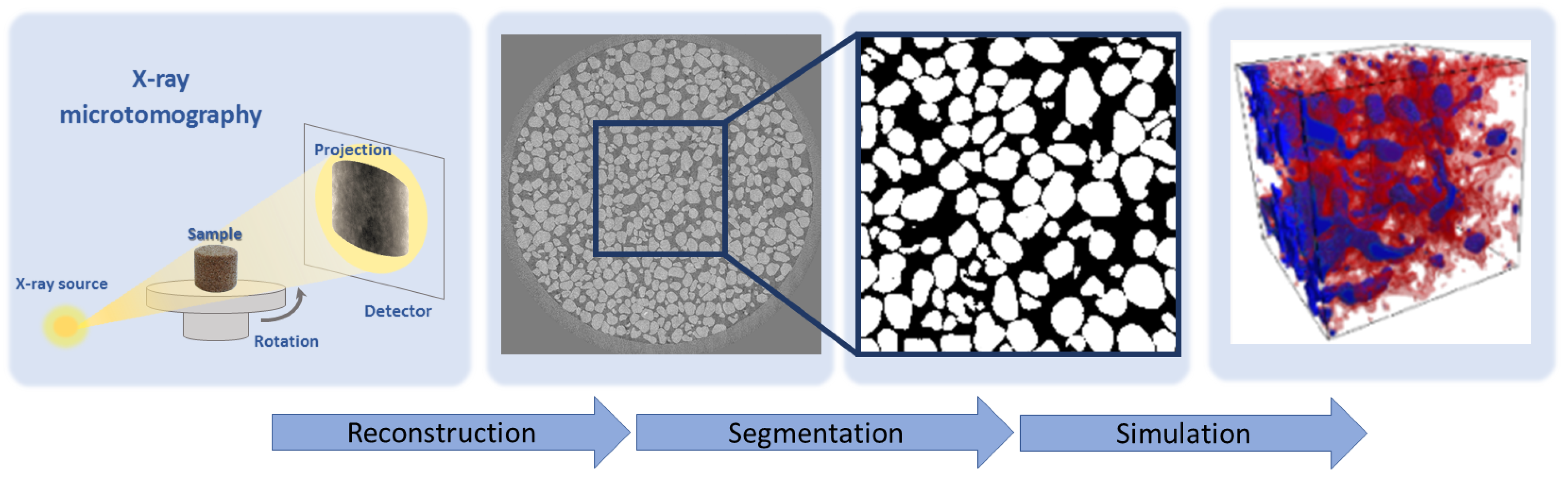
Figure 1 shows a typical DR workflow [11]. The first step is image acquisition by X-ray microcomputed tomography (microCT) [12]. The microCT system acquires a series of shadow projections over 180 or 360 rock sample rotation. A special software program reconstructs a 3D grayscale image from those projections by a back-projection method [13]. Quality of 3D image depends on the number of projections used in the reconstruction procedure. One of the key steps in the workflow is a digital model construction by segmenting a 3D image. In an ideal case, multi-class segmentation is required to distinguish different mineral phases, organic substances, and pores. For the sake of simplicity, binary segmentation is often considered: each voxel is treated as belonging to a solid matrix or pore space. The resulting digital 3D model is applied for numerical simulation of properties of interest.
Even though image segmentation has been a field of active research for many decades, it remains one of the most difficult steps in various image processing systems. In the DR workflow, inadequate segmentation yields vastly differing results in a fluid transport and geophysical modelling. It is worth noting that some level of uncertainty about a segmentation outcome is inevitable for X-ray microCT images due to many factors, in particular, partial volume effect [14]. According to our own experiments and outcomes claimed in [15,16], the Indicator Kriging (IK) algorithm [17] provides reasonable segmentation outcomes for the majority of X-ray microtomographic images and, in many cases, outperforms other segmentation techniques. However, IK requires operator participation. Parameters of IK such as two thresholds and radius of Kriging window should be selected manually for each image under processing. Usually, an operator makes several segmentation attempts to select suitable parameters. This is a long and subjective procedure even for experienced persons. Ultimately, it is desirable to have a fully automatic image processing pipeline including segmentation. It can provide improved reproducibility and more objective simulation outcomes due to excluding subjective assessments of an operator. Modern machine learning (ML) based image segmentation methods look like a perfect candidate for the role.
Nowadays, ML and especially deep learning approaches are experiencing explosive growth. The main advantage of a deep learning is the ability to learn complex patterns and features from the data itself. Segmentation by means of Convolutional Neural Networks (CNN) provides state-of-the-art results for many tasks [18]. CNN is one of the most promising approaches for automatic segmentation of microCT images. Our aim is to train CNN-based models once and to apply these models many times in the automatic mode for the segmentation of various rock samples.
One of the key challenges for the use of supervised machine learning for microCT images of rock samples is the lack of ground truth (GT). Manual pixel-perfect labelling of a large enough 3D dataset would be way too time-consuming, while utilizing significantly higher-resolution images, such as Scanning Electron Microscopy (SEM), possesses its own challenges [19,20,21]. Moreover, gathering a representative enough collection of all the practically important diverse sample types is a demanding task by itself.
In this paper, we propose an approach for generation of labelled datasets and compare segmentation results by various deep neural networks, highlighting most promising approaches and discussing potential pitfalls for automatic processing of 3D images of rock samples. The remainder of this paper is organized as follows. Section 2 contains a review of the existing approaches for segmentation of rock samples by supervised machine learning techniques. Next, we present in detail our approach for generation of training and validation datasets (Section 3), pre-processing of microCT images and training of 2D slice-wise SegNet, 2D and 3D U-net for segmentation (Section 4). Section 5 presents the experimental results for deep neural networks under investigation as well as comparison with conventional segmentation methods: IK and thresholding. Finally, the conclusions and discussions of further research directions are contained in Section 6.
2. Related Works
Training, tuning, and evaluation of segmentation algorithms for microCT images of porous media are challenging due to the lack of GT. Traditionally, samples with known spatial structure or synthetic images are applied as GT. In [16], the researchers used porosity measurements for glass beads to quantitatively compare segmentation methods. In [15], the authors simulated 2D and 3D soil images.
In this section, we focus on the review of existing applications of machine-learning techniques for handling microCT rock samples. We pay special attention to the training, testing, and validation sets construction. Data from the training set is applied for training of the ML model, data from the testing set is used for model hyperparameters adjustment, and data from the validation set is employed for the final estimation of the model performance. Sometimes, the same data are used as both testing and validation datasets.
ML-based methods of processing of microCT rock images can be divided into two groups: end-to-end regression providing direct prediction of the physical properties, such as porosity and permeability; image segmentation by solving of the classification problem with subsequent physical properties’ evaluation. We are interested in the second one because it is more interpretable and physically correct. Nevertheless, below, we mention several end-to-end methods for direct prediction of rock properties.
The authors in [22] depict the application of three unsupervised and four supervised ML methods for segmentation of three microCT images: andesite and two sandstones. Similar investigation for andesite can be found in [23]. These papers claim that the datasets they use contain up to 42 million of voxels, but each rock sample is analysed separately from all other rock types. Unfortunately, the way of splitting on training and testing datasets is described rather vaguely. According to the example, provided in the figures and in the text, all these voxels are from a single 1800 × 1800 × 10 box-shaped Region of Interest (ROI). This might not be an issue for the neural network they use (single hidden layer with just 10 neurons) but might lead to severe overfitting for larger neural networks, since even the first and the last z-slices are quite similar. Moreover, one of the difficulties, associated with cone-beam 3D microCT images we deal with, is that their local properties (e.g., sharpness) are not completely uniform—the z-slice from centre of the image is generally sharper than those from the most upper or lower part of the image. To achieve better results, one must use a dataset representing all such parts. The porosity of segmented images is compared with laboratory measurements by a gas pycnometer. Such method of estimation of segmentation quality was criticized, for example, in [11] because microCT images are limited in spatial resolution by the order of microns without any chance to reproduce pores of nanometer scale. Thus, for almost any natural rock sample, digital porosity would be lower than those measured in the lab by gas. In addition, these images are typically taken on much smaller samples than ones used for laboratory measurements, which makes direct comparison of porosity values unfair.
In [24], end-to-end CNN for prediction of pores media characteristics from images is described. Three samples of different sandstones are considered. The images of the samples are segmented by thresholding with automatic threshold selection by Otsu [25]; then, pore networks are extracted [26]. The characteristics of pores media, namely porosity, coordination number, and average pore size, are calculated from the pore networks. CNN is trained to predict the sample characteristics mentioned, based solely on 2D (128 × 128) grayscale image fragments. The dataset containing 7680 slices from images of three samples is split into training and testing ones. There are no details about the splitting procedure. We surmise that slices from each of the three samples were both in training and testing sets, and it might lead to an overestimation of the quality of the regression model.
The authors in [27] describe the application of several ML-based approaches including 2D CNN inspired by VGG (Visual Geometry Group) [28] and 3D CNN inspired by VoxNet [29] for prediction of permeability. The dataset is based solely on a single 400 × 400 × 400 image of sandstone. In one of the experiments, it was cut into 9261 intersecting 100 × 100 × 100 volumes. Not surprisingly, for such idealistic conditions, methods considered in the paper demonstrate good prediction accuracy. It would be interesting to assess their performance on unseen data.
The authors in [30] compare three methods for segmentation of synthetic microCT data. A real image of a single sandstone sample is segmented into void and solid phases via ZEISS ZEN Intellesis (Carl Zeiss Microscopy GmbH: Jena, Germany) [30]—graphical interface for interactive training of machine learning classifiers provided by scikit-learn [31] backend. For the generation of synthetic images, this segmented volume is forward-projected into the projection domain, then shadow projections are blurred, and Gaussian noise is added to them; finally, a new volumetric image is reconstructed form these processed shadow projections. A similar method for GT generation is described in [11]. Obviously, such approaches produce significantly more natural distortions, compared to adding Gaussian noise directly into the microCT image. However, a microCT device demonstrates many other distortions: X-ray tube instabilities, sample position mechanical volatility, detector dead pixels, etc. Modern reconstruction methods go to great lengths to compensate them. For example, the authors in [32] describes a method for software shadow projections post-alignment. However, even these methods are not perfect. Creating a completely synthetic dataset that would accurately reproduce all these effects is a difficult task. Moreover, even an imaginary perfect microCT device would experience phase-contrast effects that are usually visible as oversharpened edges in microCT image [33]. Basic forward and backward-projection methods ignore this effect as well.
Multi-phase segmentation of microCT image of sandstone by CNN is presented in [34]. Two versions of SegNet [35,36] in 2D slice-wise mode were explored. Just 20 slices with size 256 × 256 were annotated in semiautomatic manner. Most of the five phases are clearly distinguishable by their grayscale levels, which greatly simplifies the task. The additional phase related to “other minerals (mainly clays)” is not far from quartz by its greyscale level but features a dramatically different texture. Dataset was split into training, testing, and validation set. To cope with the limited number of annotated data available, data augmentation by cross-correlation simulation algorithm was applied.
In general, we conclude that existing works related to microCT images for Digital Rock workflow only deal with relatively small datasets. In addition, as a rule, data from the same sample are used for training, testing, and validation. Although this allows for performing a segmentation of the sample in question, it is difficult to say something about the generalization capability. The trained network might either perfectly work or completely fail on an image of another sample, which is different by mineralogy, image acquisition parameters, intensity distribution, etc.
3. Datasets
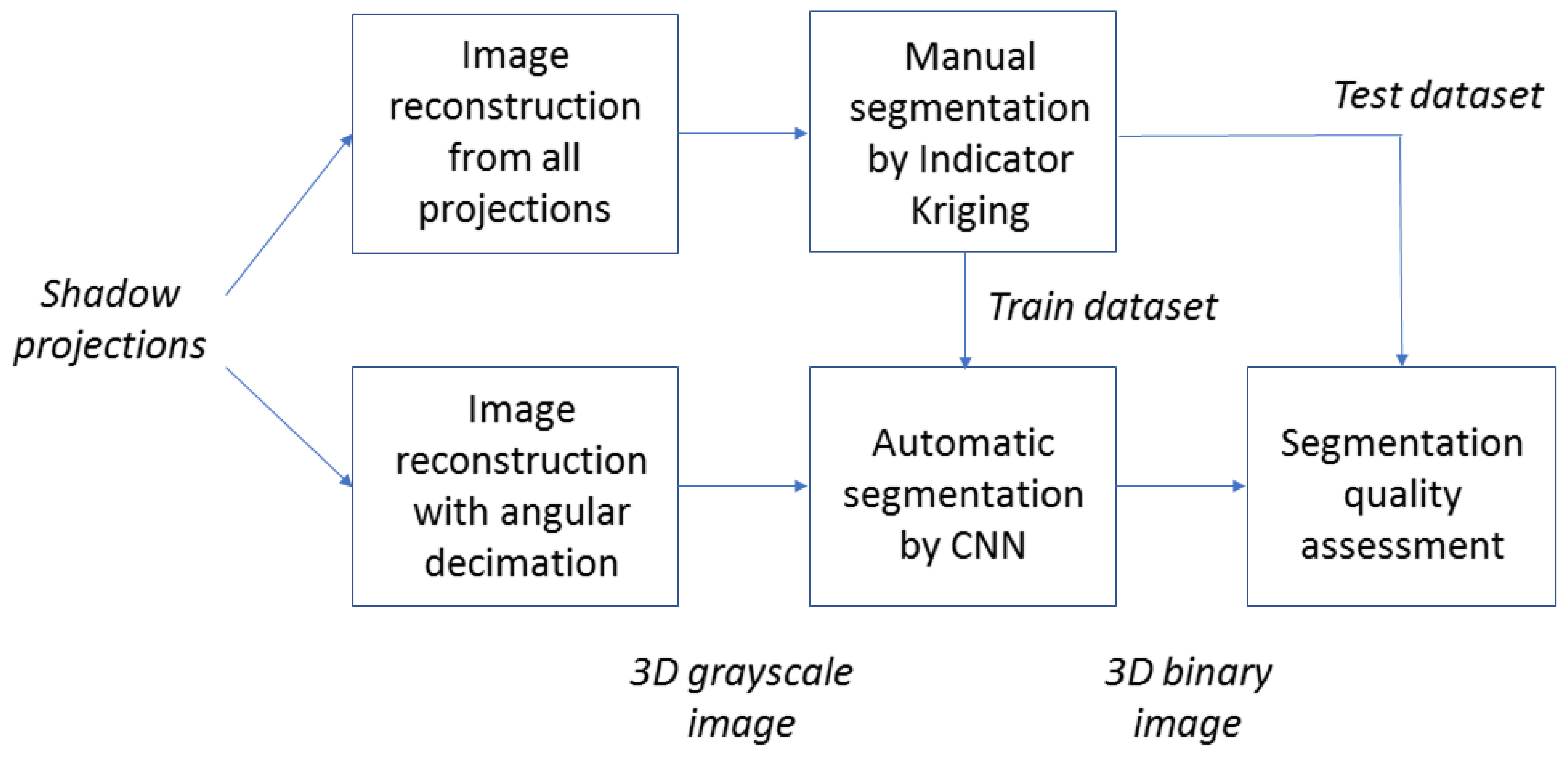
We propose the following relatively fast and simple approach for dataset generation. Our aim is to achieve the maximum possible quality, even if the experiment will last several times longer than a standard one. It should be noted that enormous increase of imaging experiment time does not guarantee perfect quality by itself. Possible instabilities of microCT system can lead to significant degradation of overall image quality for long scanning. First, an X-ray microCT experiment with a reasonably large number of shadow projections is conducted. High-quality 3D grayscale image is reconstructed using all shadow projections. Next, we run the same reconstruction process using only each forth projection to produce the 3D grayscale image with reduced quality. Such approach is named angular decimation. Finally, we perform IK-based segmentation of the high-quality grayscale image and obtain the binary image, which we consider as GT for image with reduced quality. IK parameters are thoughtfully selected by an operator in an interactive manner. The dataset is split into training and validation sets. Figure 2 demonstrates the scheme of our approach for datasets generation and investigation of microCT images’ segmentation methods.
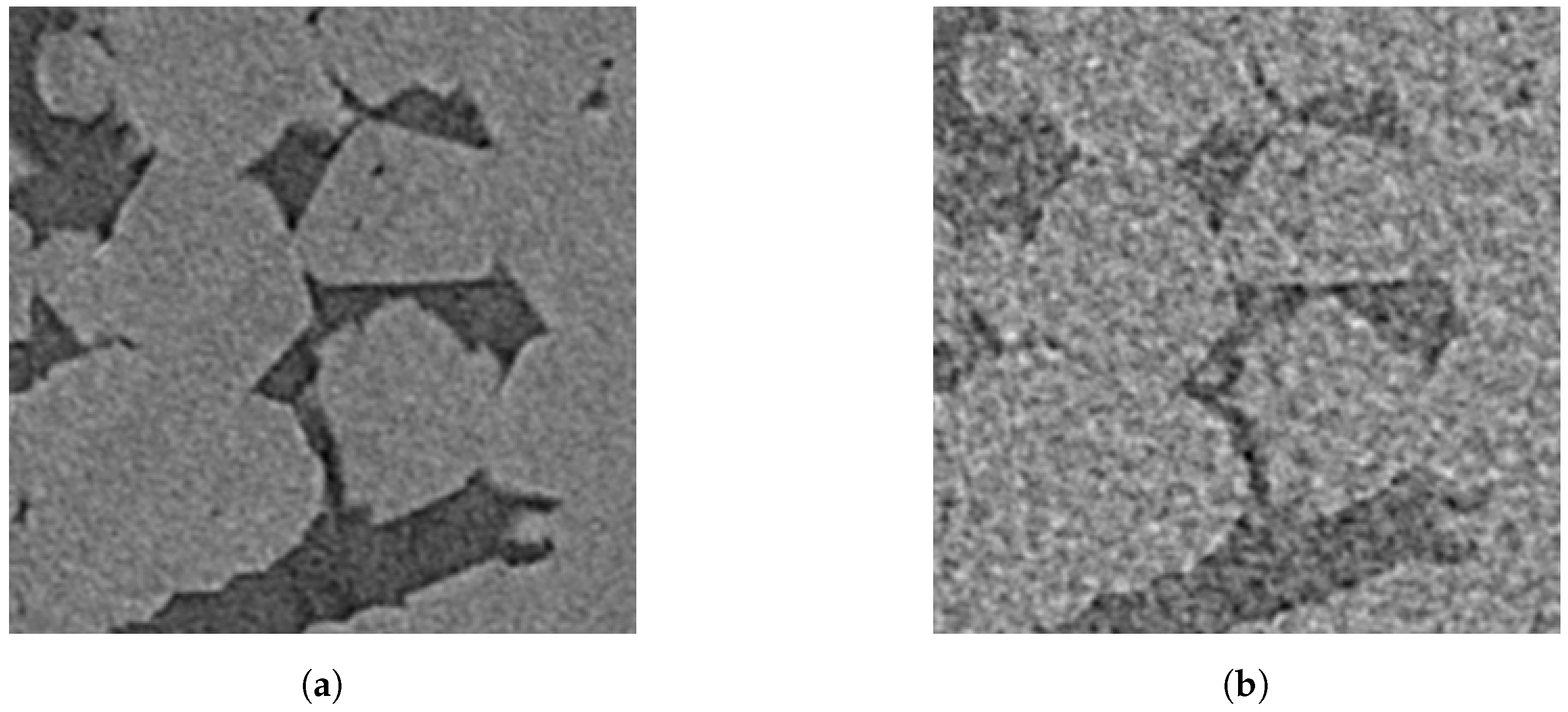
One can compare the quality of corresponding image fragments reconstructed from all shadow projections (see Figure 3a) and reconstructed from four times less shadow projections (see Figure 3b). The usage of the reduced number of shadow projections can be considered as a mimicking of a faster way of scanning. This decimated set of the shadow projections is highly similar to independent four times faster scan. In contrast to unnatural noise patterns and hardly-realistic ring artefacts demonstrated in [11], our images reconstructed with four times angular decimation demonstrate no unnatural features.
Our assumption is the following: the best technique performs segmentation of the worsened copy as much as possible closer to segmentation outcomes for high-quality ones. For our experiments, we selected eight samples of sand and sandstones, which can be scanned with the best quality to mitigate dependence from the segmentation method for GT obtaining. Although we apply our own modification of the IK algorithm for the segmentation of high-quality images, any reasonable segmentation technique could be used for the task. We also use IK for comparison with CNN-based segmentations. We argue that IK has no intrinsic advantages over other techniques under investigation because the statistical distributions of intensities in the local vicinity notably differ for an image with reduced quality and a high-quality one.
We scanned the samples using SkyScan 1172 microCT system (Bruker MicroCT: Kontich, Belgium) with the following parameters: X-ray high voltage—100 kV, X-ray tube current—100 A; voxel size—2.3 m; exposure time—1767 ms, averaging of 10 frames. The imaging was performed in 180 mode, and about 2000 shadow projections were employed for reconstruction of a high-quality image.
The samples belong to five different types:
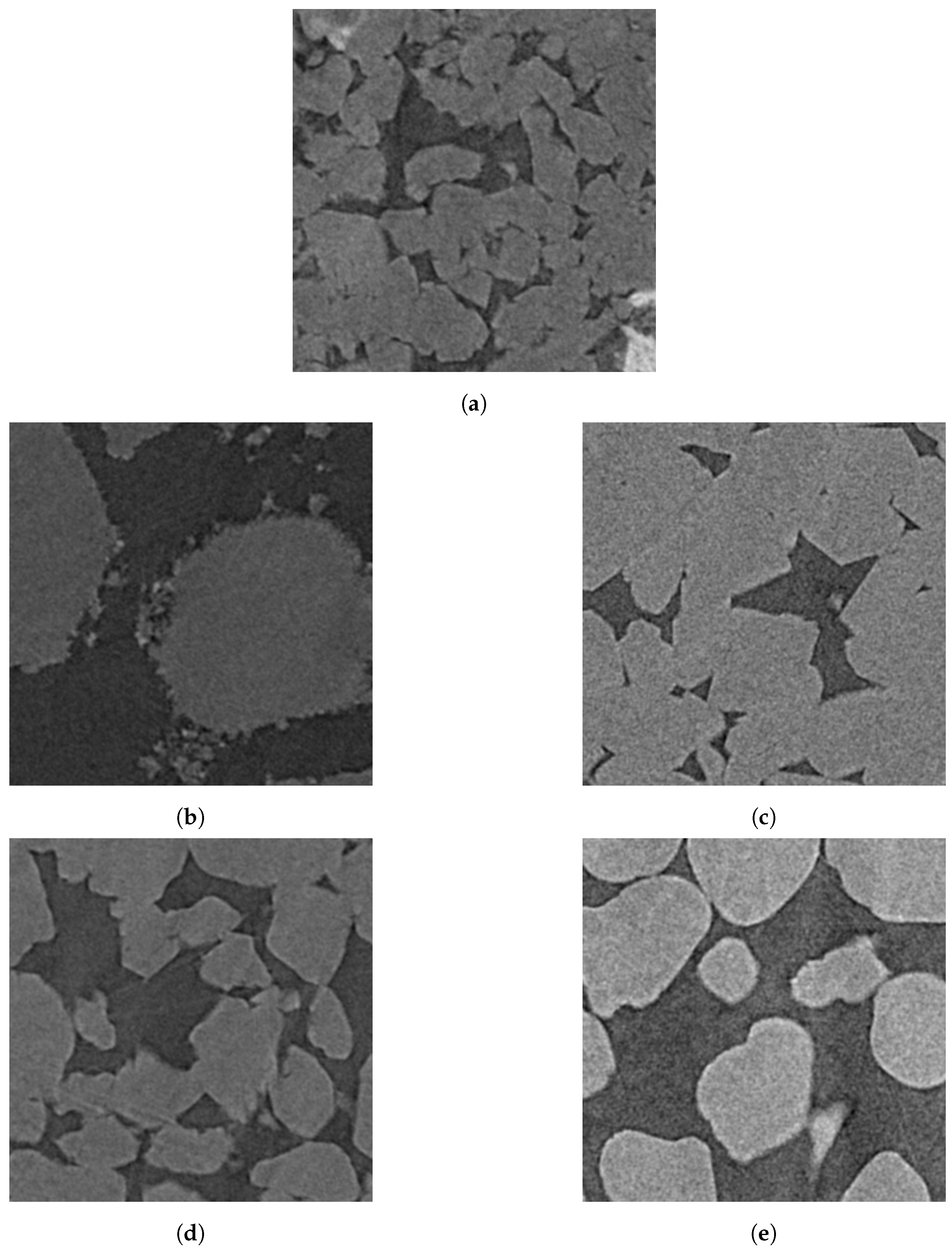
- BB: Buff Berea sandstone has small semi-rounded non-uniform grains (see fragment of high-quality image in Figure 4a).
- GRV: Gravelite sandstone has large angular non-uniform grains (see a fragment of a high-quality image in Figure 4b).
- FB: Fontainebleau sandstone has large angular uniform grains and almost no microporosity (see fragment of high-quality image in Figure 4c). We used two samples of such sandstone denoted as FB1 and FB2.
- BHI: Bentheimer sandstone has middle, sub-angular non-uniform grains with 10–15% inclusions of other substances such as spar and clay (see fragments of high-quality images in Figure 4d). We used three samples of such sandstone denoted as BHI1, BHI2 and BHI3.
- UFS: Unifrac sand has large rounded uniform particles and no microporosity (see fragments of high-quality images in Figure 4e).
In this paper, we use the microporosity term for the designation of fine structures relating to pores and grains having a size close to scanning resolution.
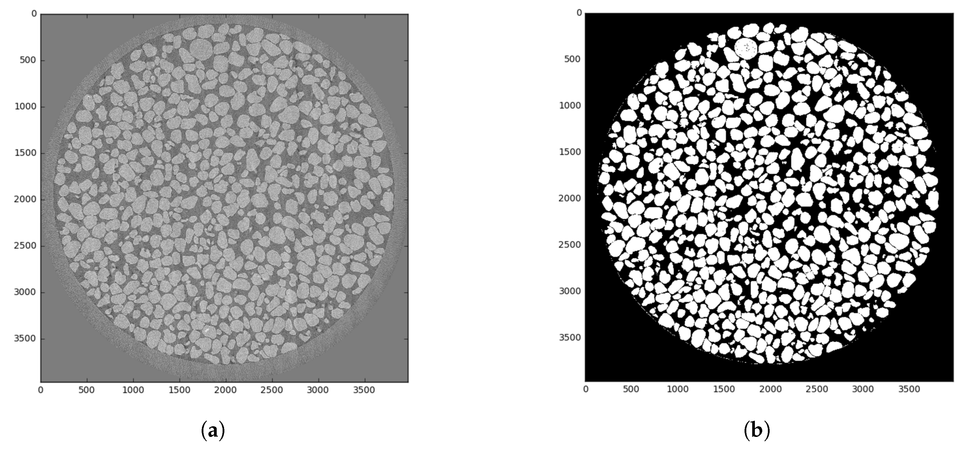
Each 3D image has a size of voxels with 8 bits per voxel bit depth. It can be represented as a set of matrices and . Ground truth segmentation can be represented as a set of matrices and . Figure 5a shows an example of a slice for a UFS sample, and Figure 5b demonstrates corresponding GT. Brighter pixels refer to a more solid matter. For the segmented image, white pixels stand for quartz, and black pixels are for voids. We only consider the inner part of the image belonging to a sample. Thus, we process for each 3D image about 1600 slices containing a totally voxels per image.
As was mentioned above, existing studies of applications of machine learning techniques for segmentation only use from one to three samples of rocks. It leads to an overestimation of segmentation quality and does not allow assessment of the generalization capability of trained classifiers. We have no aim just to demonstrate that CNN is able to provide high segmentation outcomes for the single sample, in the case of the network being trained on the same sample. Our intention is the investigation of how CNN-based segmentation operates for unseen data:
- unseen rock types,
- unseen samples of rock types represented in the training set.
On the other hand, we aim to maintain a reasonably limited rock types variability. We do not include carbonate rocks, X-ray contrasted samples, etc.
We split our dataset into training and validation sets in five different ways (see Table 1). We do not fine-tune hyperparameters individually for each experiment, so we do not use the testing dataset. Dataset 1 is aimed at the estimation of segmentation quality of sandstones by a neural network trained on a single UFS sample. Datasets 2 and 3 have one additional sample in the training set. Dataset 2 includes GRV, which has maximal visual difference with other images, in the training set. Dataset 3 includes FB1 to training set, and it has GRV and FB2 (second sample of Fontainebleau sandstone) in the validation set. Dataset 4 includes UFC, GRV, and FB1 in the training set. Finally, Dataset 5 has five samples in the training set and FB2, BHI3, and BB in validation set. In general, we expect an improvement of the performance of neural networks with enrichment of the training dataset with the new data.
As mentioned above, existing investigations of the application of machine learning methods for the segmentation of images of rock samples used relatively small training and testing sets. Our datasets significantly outperform them in both the amount and diversity of data. Table 2 contains sizes of training and validation sets in 3D images, 2D slices, and voxels.
4. Explored CNN Architectures
4.1. Segmentation of Volumetric Images by CNN
In image segmentation, the current state-of-the-art results are frequently obtained using the deep learning approach. The success of the neural networks started with [37]. It explains basic techniques and intuition of neural networks and their application to computer vision problems. Fully convolutional neural networks [38,39] are among the most successful methods. Magnetic resonance imaging (MRI) and connectome imaging are yet other examples of widely studied image modalities, somewhat similar to rock sample microCT images. Recently, several CNN-based architectures for segmentation of 3D biomedical images were proposed [40,41,42,43,44,45,46,47,48]. It is worth noting that the majority of analysed publications describes various modifications of U-net or SegNet networks [35,36,49]. In addition, modern algorithms sometimes exploit a combination of a deep learning approach with some other techniques, for instance, Conditional Random Field [50].
Based on literature analysis and our preliminary experiments, we decided to estimate performance of the following deep networks for segmentation of rock images from our five datasets:
- 2D SegNet for processing microCT image in slice-wise mode;
- 2D U-net for processing microCT image in slice-wise mode;
- 3D U-net for processing microCT image in 3D mode.
4.2. Pre-Processing
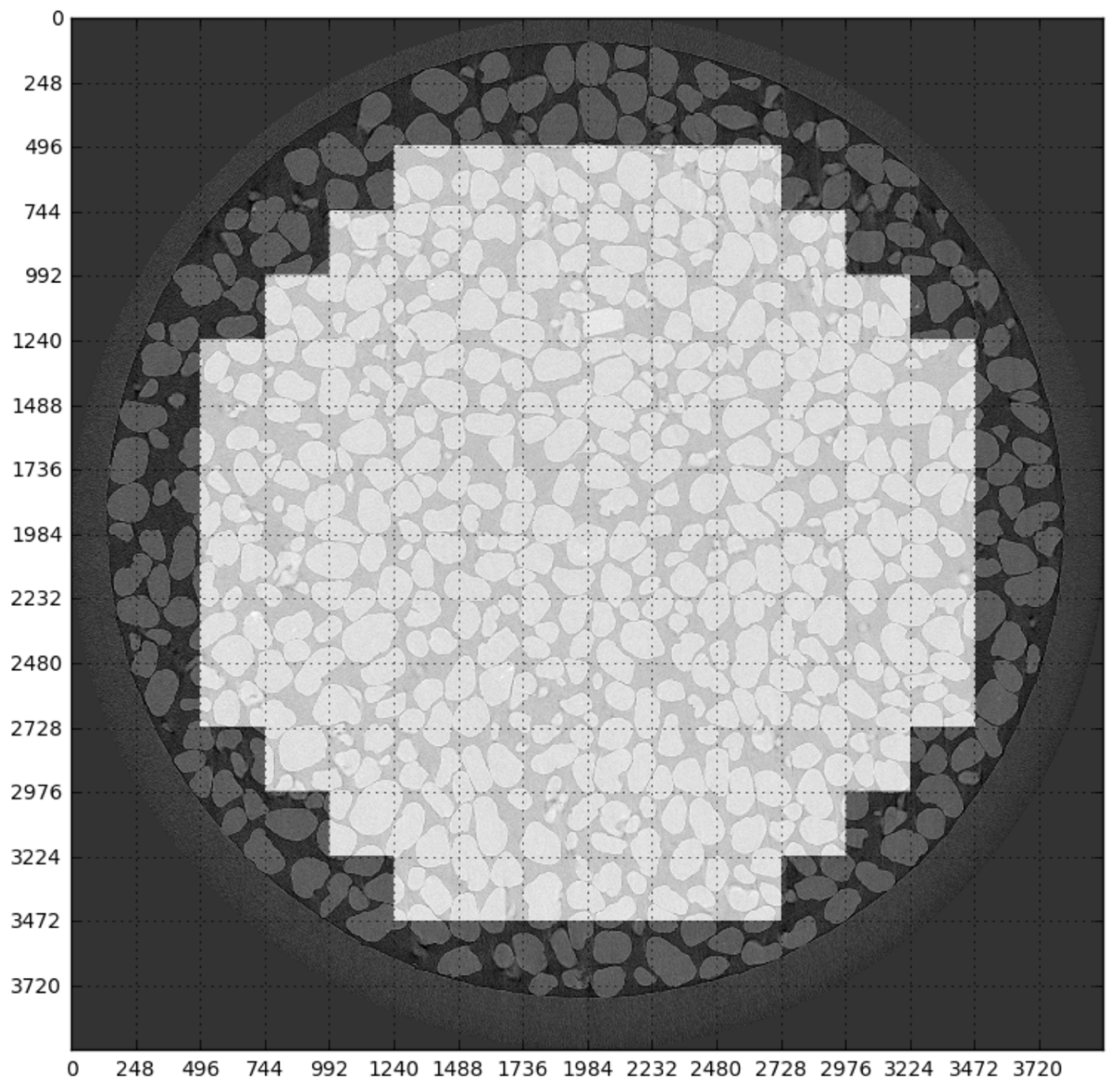
All our rock samples are cylindrically shaped and occupy the central part of each z-slice. Corners of the slice can contain different intensity of pixels depending on the microCT system and regardless of the actual data. In addition, a sample can be placed in a holder. We only process the inner part of the image belonging to a sample, a so called, Region of Interest (ROI). For our dataset, we set up ROI manually, although the approach for automatic ROI selection [51] can be applied as well. We use patches from the ROI of an original image for training and inference. For 2D networks, the patch size is pixels. As a sort of data augmentation, we sample patches with stride 248 on both axes. Squares in light tone in Figure 6 illustrate selected patches. For a 3D network, we use non-overlapping patches.
Next, the step for data pre-processing is an intensity normalization. Distributions of pixel intensities strongly differ for each rock types. To reduce this difference, we perform normalization as follows. Under the assumption that each distribution is a mixture of two normal distributions (one for air and one for quartz), we estimate parameters of this distribution using expectation–maximization (EM) algorithm [52]. Then, we apply the following transformation:
where are mean values of normal distributions; x is intensity of a voxel of original image; is normalized voxel intensity.
4.3. SegNet
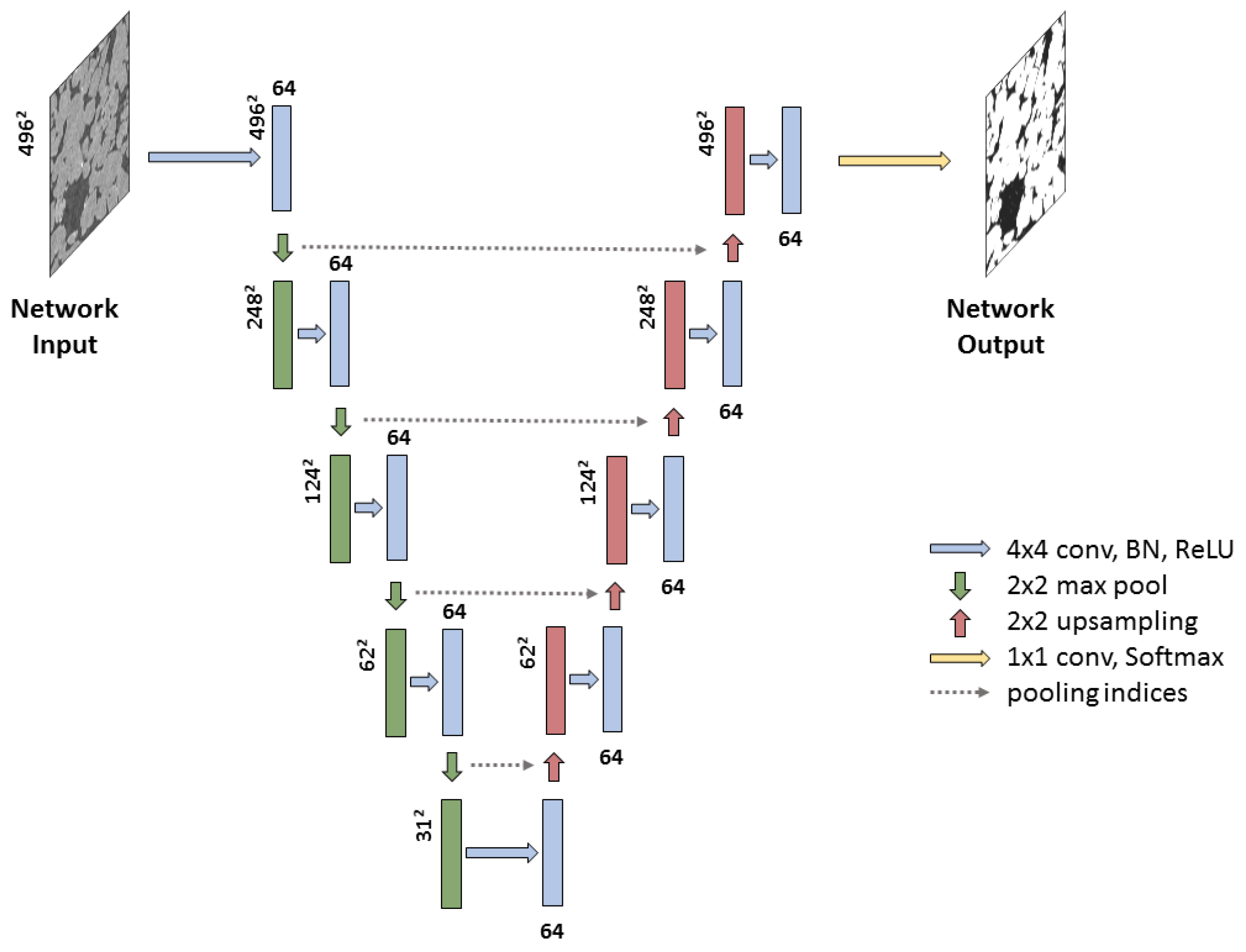
SegNet [35,36] is a fully convolutional neural network that consists of two parts: (1) convolutions and downsampling (encoding) and (2) convolutions and upsampling (decoding). Convolution, downsampling and upsampling are the most important parts of fully convolutional neural nets for semantic segmentation. SegNet architecture is shown in Figure 7.
The encoding part of SegNet consists of several encoder units. Each encoder performs convolution with a filter bank to produce a set of feature maps. The first filter bank (blue arrow) operates on patches 496 × 496 pixels () from the original microCT image and consists of 64 filters. Its output is shown as a blue block with the same spatial size () and 64 feature channels (shown on top of the block). These maps are batch normalized [53]. After normalization, an element-wise rectified linear unit (ReLU) is used. Following that, max-pooling with a window and stride 2 (non-overlapping window) is performed, so the resulting output is sub-sampled by a factor of 2. Max-pooling allows for achieving some translation invariance for tiny spatial shifts in the input image and increases the receptive field of the subsequent layers. On the other hand, max-pooling results in a loss of spatial resolution. Decoding part of SegNet consists of several decoder units. Decoder unit upsamples its input feature map using the memorized max-pooling indices from the corresponding encoder feature map. This step produces sparse feature map. The feature maps are then convolved with a trainable decoder filter bank to produce dense feature maps. The high-dimensional feature representation at the output of the final decoder is fed to softmax. The output of the softmax layer is a K channel image representing class probabilities, where K is the number of classes. For each pixel, the predicted class corresponds to the channel with the maximum probability. In our case, K equals two.
The remaining parameters are:
- Objective function is log-loss.
- The optimization method is stochastic gradient descent (SGD) with momentum (, ).
- regularization of all parameters with weight .
- Batch size equals 1.
- Number of iterations during training is selected as follows. Every 100 iterations, we evaluate accuracy on hold-out set ( of patches for each rock sample) and stop the training, when accuracy stabilizes. In this experiment, accuracy stabilized when number of iterations reaches about 3000.
4.4. 2D U-Net
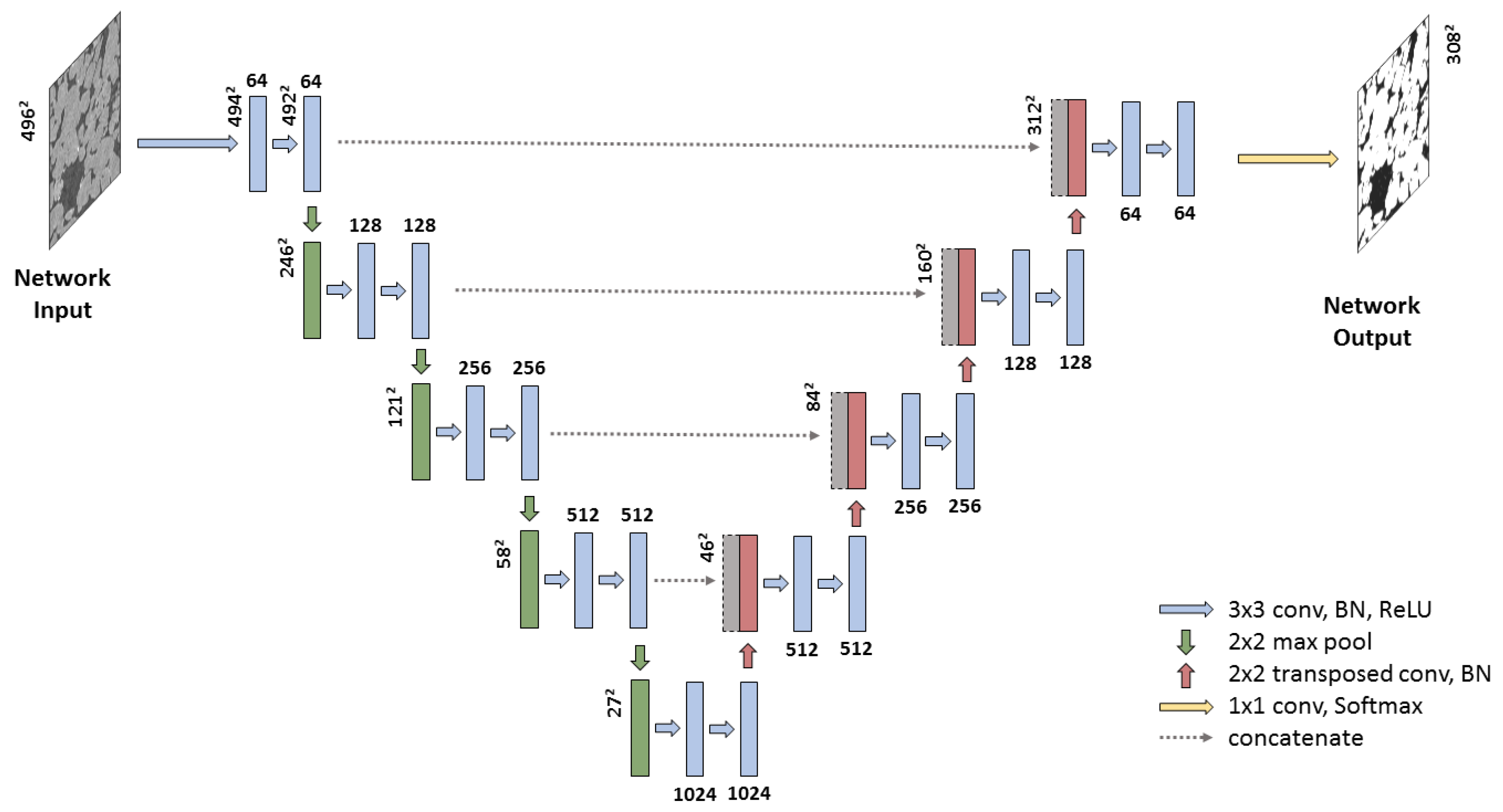
U-net [49] has achieved state-of-the-art quality on many biomedical image segmentation tasks. The network architecture is illustrated in Figure 8. The encoding part follows the typical architecture of a convolutional network. It consists of the repeated encoder units each of which consist of two valid (or unpadded) convolutions, each followed by a rectified linear unit (ReLU) and a max pooling operation with stride 2 for downsampling. Each encoder doubles the number of feature channels. The decoder part of U-net also consists of several decoder units. Every decoder consists of up-convolution layer that halves the number of features channels and doubles spatial resolution of each feature map, a concatenation with the correspondingly cropped feature map from the contracting path, and two convolutions, each followed by a ReLU. The cropping is necessary due to the loss of border pixels on every convolution. Up-convolution layer is the same as in DeConv net [39]. At the final layer, a convolution is used to map each 64-component feature vector to the desired number of classes.
In our experiments, we apply one modification to the original architecture, and we add batch normalization layer before each ReLU unit in the original U-net. It significantly improves convergence speed. Learning rate was chosen small enough for convergence, batch size was chosen as large as GPU memory allows. The rest of training parameters are the following:
- Objective function is log-loss.
- The optimization method is stochastic gradient descent with momentum (, ). In addition, exponential decay is applied—every 6000 iterations, the learning rate is multiplied by .
- Batch size equals 16.
- Number of iterations during training is selected as follows. Every 100 iterations, we evaluate accuracy for the next batch. The training is stopped when accuracy becomes constant. In this experiment, accuracy stabilized when the number of iterations reaches about .
4.5. 3D U-Net
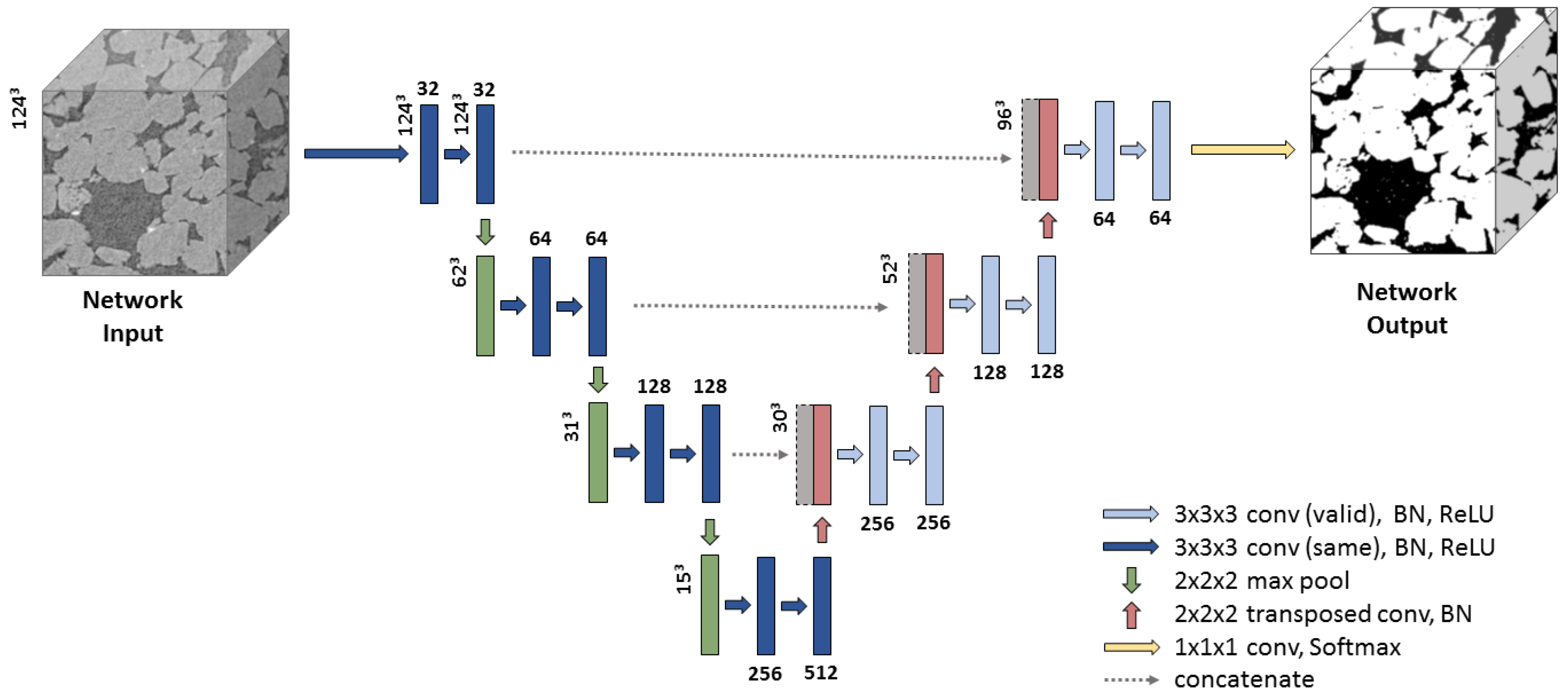
We expected that explicitly taking the 3D nature of the image into account would improve the performance of our model. Replacing all 2D operations, such as convolution, max pooling, etc, with their 3D counterparts allows for reusing the 2D network architecture. The 3D U-net network architecture is illustrated in Figure 9.
Again, we have two parts: encoding and decoding. The encoding part follows the typical architecture of a convolutional network. It consists of the repeated encoder units, each of which consists of two convolutions, followed by a batch normalization and then rectified linear unit (ReLU) and a max pooling operation with stride 2 (along each axis) for downsampling. We keep the number of feature channels the same after first convolution and double it after second convolution. Taking into account GPU memory limitations, we use the same convolutions in the encoding part, i.e., we keep the same spatial size after each convolution. The decoder part of the 3D U-net also consists of several decoder units. Every decoder contains: up-convolution layer that keeps the number of feature channels the same and doubles spatial sizes of each feature map; a concatenation with the correspondingly cropped feature map from the contracting path; and two convolutions, each followed by a batch normalization and ReLU. The cropping is necessary due to the loss of border pixels in every convolution. The up-convolution layer is similar to the 2D case and works as follows: for each pixel in input tensor, up-convolution provides a tensor by multiplying the value of this pixel on a trainable kernel with shape .
For the 3D U-net, only a single patch fits into the GPU memory. The training parameters are listed below:
- Objective function is log-loss.
- The optimization method is stochastic gradient descent with momentum (, ). In addition, exponential decay is applied—every 2000 iterations, the learning rate is multiplied by .
- Batch size equals 1.
- Number of iterations during training is selected as follows: every 100 iterations, we evaluate accuracy for the next batch. The training is stopped when accuracy becomes constant. In this experiment, the number of iterations was about 6000.
5. Results and Discussion
For evaluating the quality of the segmentation inside ROI, we decided to pick the most application-neutral metrics, Accuracy expressed in percentages:
where are indices of pixel; ROI is the region of interest depicted in Figure 6; l is the number of slices; is the matrix of predicted labels; S is the matrix of ground truth labels. The Accuracy is calculated for each sample separately.
Our aim is developing a solution for automatic segmentation without operator participation. Currently, in our Digital Rock workflow, IK operates under operator control. The image segmentation algorithm IK is based on two concepts [17]. The first concept is the kriging (or Gaussian process regression) interpolation method, which is widely used in geostatistics [54]. Kriging provides optimal (in sense of minimum variance) estimation of the unknown value at some spatial point based on the values observed in the neighbourhood points weighted according to spatial covariance. In general, the idea is associated with distance-weighting algorithms. The size of the neighbourhood is chosen by an operator. The second concept is the indicator, which represents the value to be interpolated, and is based on an a priori assignment of grayscale values to classes, for example, pore and solid substances.
Thus, the IK method requires three parameters set by an operator for the segmenting of each image. Firstly, the window radius controls the neighbourhood size. Increasing window radius usually results in a smoother and less noisy outcome. Secondly, the two thresholds are used to create indicator functions for the pore and substance classes. Ultimately, they are associated with probabilities that a voxel with a given intensity level belongs to a specific class if ignoring all the information about its neighbours. The simplest interpretation is that all pixels above the substance threshold should go to the substance class, regardless of their neighbourhood and vice versa all below the pore threshold go to pore class. Selecting adequate thresholds is especially challenging for noisy images when the noise level exceeds the difference between the grey levels associated with the two classes.
Even for an experienced person, it is extremely difficult to select these three parameters for providing suitable segmentation results from the first attempt. In practice, operator iteratively makes several segmentation attempts aiming to find better parameters based on visual analysis of results. For considered images, such iterative parameter selection by operator requires about an hour. Despite several attempts, segmentation results remain rather subjective, and their repeatability and reproducibility are not high.
Table 3 contains Accuracy of segmentation via IK by three operators. These results were obtained for a BB image reconstructed with four times angular decimation. Each operator made five attempts. In these attempts, one can see a huge spread in segmentation quality. Although theoretically achievable Accuracy by IK for this image equals 96.2, no one from the operator did not get this optimal result, average Accuracy in operators’ attempts is much lower than the highest possible. For the other seven images, we could not organize identical manual segmentation experiments via IK by experienced operators. Instead of that, we determined optimal IK parameters by means of Accuracy maximization via a simplex search optimizer [55].
In spite of its simplicity, there are examples of successful applications of thresholding for segmentation of microCT images [2,56]. Thresholding is applicable in the case of high contrast between voxels of voids and solid substances, which leads to the bi-modal histogram. In the thresholding algorithm, the voxels with a value lower than or equal to the threshold are marked as pore and voxels with a value higher than the threshold are marketed as a solid. In practice, the threshold is set by an operator or automatically [25]. We consider thresholding as one more non-machine-learning method for comparison. We determined an optimal threshold by Accuracy maximization via the exhaustive search.
Table 4 contains Accuracy of segmentation of images reconstructed with four time angular decimation for both non-machine-learning methods. In this table, IK and thresholding are thought to be the same as perfect manual parameter selection. In the most cases, interactive parameters selection by an operator would provide worse segmentation quality. Thus, one should understand Accuracy of these optimal IK and thresholding as an upper estimation of their performance.
From Table 4, we can see, as it was expected, IK provides much better results in comparison with thresholding. For IK, variation of Accuracy among different samples is very low, and IK performs equally for diverse images. For thresholding, Accuracy on the UFS sample is significantly lower in comparison with other images.
For CNN-based segmentation methods, we present results in two ways: Table 5, Table 6 and Table 7 contain Accuracy for SegNet, 2D U-net, and 3D U-net accordingly depending on dataset, and we discuss the performance of each network independently from each other; Table 8, Table 9, Table 10, Table 11 and Table 12 contain Accuracy for five datasets depending on the segmentation method, and we compare deep neural networks with each other as well as against IK and thresholding.
Table 5 contains Accuracy of segmentation by 2D SegNet depending on the dataset. The hyphen symbol means that the sample is in the training set. One might expect that adding more data to the training set should improve the segmentation quality. This should be clearly seen when the data related to the same rock type as in validation set is added to the training set. Sometimes, training set enlargement can lead to an insignificant decrease of Accuracy due to occasional stuff. For FB2 sample, Accuracy goes down as we add a GRV rock sample together with FB1 to the training set, although the addition of only FB1 leads to performance increases. Some effects do not satisfy our expectations. For BHI3, Accuracy decreases after adding BHI1 and BHI2 to training set. Moreover, Accuracy for BHI3 differs drastically from the metrics for BHI1 and BHI2. It is surprising because we do not see visual differences between those three images. In general, even without comparison with other segmentation methods, SegNet demonstrated unsatisfactory outcomes.
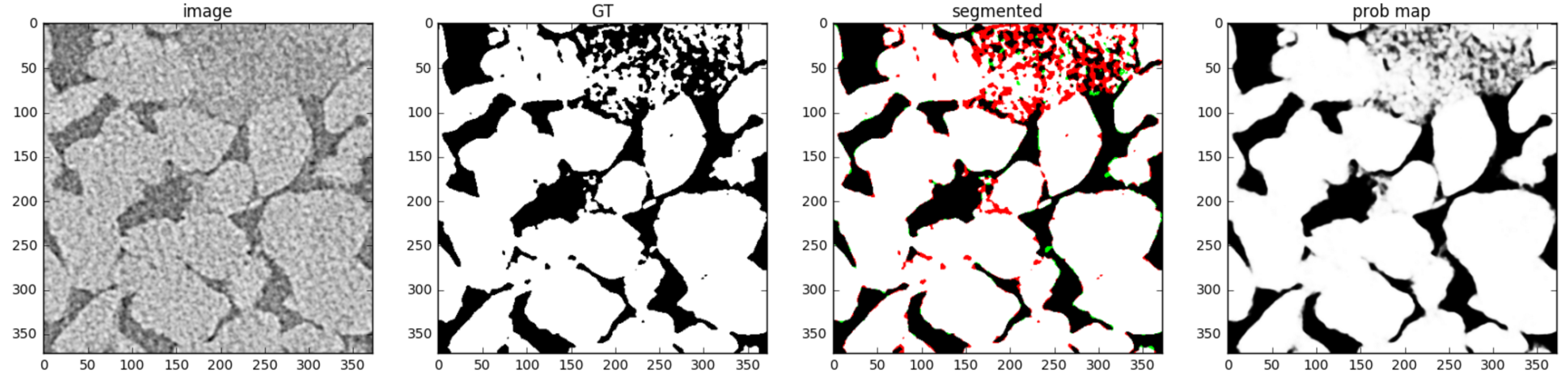
Table 6 contains Accuracy of segmentation by 2D U-net depending on the dataset. Obtained outcomes satisfy our expectations. Segmentation quality grows with the size of training set. Accuracy for FB2 increases when we include FB1 sample to the training set. The same happens for BHI3 after the adding BHI1 and BHI2 to the training set. There is no big variety in quality metrics for different samples, except Dataset 1 with the smallest training set. Figure 10 and Figure 11 demonstrate how training set enrichment affects 2D U-net segmentation quality for the most difficult clayey regions with microporosity. These figures show GT, segmentation outcomes with an indication of false positive and false negative errors, and visualization of network output, which can be treated as a posteriori probability. Regions with microporosity proved to be the most challenging for segmentation by the networks. In BHI1 image (see Figure 4e), the entire microporosity region was segmented erroneously by a network trained on Dataset 1 that only contains a rounded and non-microporous UFS sand sample (see Figure 4e) in the training set. The probability map looks much like a binary image; most pixels are close to either zero or one. The microporosity region is not only incorrectly classified, but the network is pretty sure that this is a large almost clean pore. When we enrich our training set with GRV and FB1 sandstones, which have some regions with microporosity, the situation becomes better (see Figure 11). Once again, the majority of the segmentation errors are located in the microporosity region; however, the probability map demonstrates shades of grey there, and some of pixels are predicted properly. Indeed, these pixels are difficult to predict.
Segmentation outcomes by 3D U-net are presented in Table 7. As well as for 2D U-net, we do not see any contradictions in the results by 3D U-net.
Let’s compare various segmentation methods (see Table 8, Table 9, Table 10, Table 11 and Table 12). SegNet performance is clearly inferior to the other methods. Accuracy of thresholding is not high even for an optimal threshold. Formally, IK with optimal parameters has the highest segmentation quality. In practice, IK with parameters selected by an operator can have a lower performance (see Table 3). Taking into account the performance of IK “in wild”, 2D and 3D U-net provide comparable results, sometimes these networks outperform IK. The undoubted advantage of U-net-based methods is operator-free segmentation mode. Once trained, we are able to use the model without adjustment of any parameters. 2D and 3D U-nets provide perfect repeatability and reproducibility segmentation results. The application of these deep networks excludes the influence of the subjective judgments of an operator.
Since a 2D segmentation technique is unable to use all available local information, our intuition suggests that we should use 3D receptive fields. However, 2D and 3D U-nets performance is approximately equal. This could be related to by the restrictions, imposed on the 3D model, to limit the computational cost: the smaller number of layers and feature maps, padding, etc. This phenomenon can be explained by the small depth of 3D model and relatively small size of 3D cube used for training and inference; recall that we cannot expand our network due to GPU memory limits. The authors in [43] compare 2D and 3D U-net for segmentation of cardiac MRI images and make a similar explanation to the fact that the 3D network does not outperform the slice-wise one. We expect that further thoughtful architectural and hyperparameter optimizations would eventually allow the 3D version to outperform the 2D one.
In addition, our study suggests that the optimal choice of the quality metrics remains an open issue. Pixel-wise Accuracy, being deliberately general and neutral toward different applications, has limited discrimination power for estimation of segmentation quality of images of rock samples. Experiments with images having microporosity shows big regions of solid matrix and voids providing the main contribution to the measure, whereas small structural features occurring has a subtle influence. However, such microstructural features can have significant importance for further simulation, e.g., of flow processes. It is preferable to elaborate quality metrics based on physical meanings of pore space topology and roughness of surface for the problem solved.
All experiments were performed on a system with four GPUs Tesla K40m made by nVidia (Santa Clara, CA). GPU provides 2880 stream cores, 12 GB of memory, and 4.29 Tflops of peak single precision performance. All CNNs were implemented via TensorFlow [57]. Each of the CNN-based models was independently trained on each of the five datasets. Typically, we did training at night. Training time for every model was about 12 hours. There is no significant difference in training time for models under consideration. Thresholding is the fastest segmentation method, and several minutes are required for processing of microCT images; however, segmentation quality is unacceptable. Segmentation time for both U-nets is about several hours per image. Taking into account several attempts of an operator to find suitable IK parameters, such segmentation time is comparable with the current segmentation procedure via IK. Using special hardware accelerators can speedup segmentation via CNN [58].
6. Conclusions
The key finding of our investigation is the following: 2D and 3D U-nets allow for automatic operator-free segmentation of microCT images of rock samples, have high generalization capability on previously unseen sample types and produce results comparable with IK controlled by an operator. Once trained, a CNN-based model is applied without adjustment of any parameters on the segmentation stage. This deep network provides perfect repeatability and reproducibility outcomes; and allows for excluding the influence of the subjective opinion of an operator. Segmentation quality of CNN depends on the presence of the visually and structurally similar samples in the training set. A software prototype developed in the scope of this research allows effective and efficient experiments, both in terms of fine-tuning of the segmentation parameters and varying available training samples. After additional adjustment and training, the CNN-based model should be used in a Digital Rock workflow, which is used for simulation of physical properties of oil-bearing rocks.
An important contribution of our research is the way for the generation of labeled datasets for training, testing, and validation of the segmentation of microCT images. First, we scan a specimen with a reasonably large number of shadow projections. High-quality 3D grayscale images are reconstructed using all shadow projections. Next, we run the same reconstruction process using a smaller number of projections to produce the 3D grayscale image with a reduced quality. Finally, we perform segmentation of this high-quality grayscale image and obtain the binary image, which is considered as a ground truth for an image with reduced quality. We apply IK for segmentation of the high-quality image, though another method providing high segmentation quality can be used as well. IK parameters are thoughtfully selected by an experienced researcher in an interactive manner.
We conclude the whole segmentation pipeline and machine learning models should be painstakingly designed. Namely, we designate the following promising directions of future work:
- To increase a generalization capability, it is necessary to do data augmentation taking into account physical principles of image forming in X-ray microtomography: model of noise, typical artefacts, parameters of reconstruction procedure, etc. Of course, common approaches of data enrichment can be used as well. In addition, one needs to find a reasonable trade-off between the amount of data and time for model training.
- Pre-processing greatly affects segmentation results. An intensity normalization by means of approximation by two Gaussian mixture is arguable even for samples with a monomineralic matrix. The authors in [14] claims distribution of monomineralic sample with pores should be modelled by three Gaussians due to partial volume effect. In practice, for the normalization of images of multi-phase samples, a more universal and robust method is required. It is worth considering some techniques for smoothing before application of neural networks for segmentation. An application of edge-preserving filtering, for example bilateral filter [59], non-local means [60], or multi-block bilateral filters [61] might be able to boost segmentation performance.
- Further optimization of the true 3D deep neural network architecture should allow for improving the segmentation quality without too large an increase in computational complexity and the number of parameters. Replacing straightforward 3D convolution layers with some kind of more sophisticated convolution blocks, e.g., inception modules [62], is one of the promising approaches.
- Post-processing of the output of neural network can eliminate some abnormalities, for example, unconnected fragments of solids inside pore space.
- Elaboration of an adequate to the physical meaning quality metric is one of the key success factors in the development of a method for segmentation of microCT images of rock samples.
Author Contributions
I.Y. was responsible for microCT images acquisition and reconstruction, the task conceptualization and project administration. I.V. created the methodology of training/validation datasets preparation as well as worked on the validation of obtained outcomes. I.S. worked on review of prior art and original draft preparation. All co-authors approved the final manuscript.
Funding
This research received no external funding.
Acknowledgments
The authors are thankful to Kirill Neklyudov for preparation of CNN-based models and Irina Reimers for help with preparation illustrations for this manuscript.
Conflicts of Interest
The authors declare no conflict of interest.
References
- Blunt, M.J.; Bijeljic, B.; Dong, H.; Gharbi, O.; Iglauer, S.; Mostaghimi, P.; Paluszny, A.; Pentland, C. Pore-scale imaging and modelling. Adv. Water Resour. 2013, 51, 197–216. [Google Scholar] [CrossRef] [Green Version]
- Andrä, H.; Combaret, N.; Dvorkin, J.; Glatt, E.; Han, J.; Kabel, M.; Keehm, Y.; Krzikalla, F.; Lee, M.; Madonna, C. Digital rock physics benchmarks—Part I: Imaging and segmentation. Comput. Geosci. 2013, 50, 25–32. [Google Scholar] [CrossRef]
- Berg, C.F.; Lopez, O.; Berland, H. Industrial applications of digital rock technology. J. Pet. Sci. Eng. 2017, 157, 131–147. [Google Scholar] [CrossRef]
- Koroteev, D.; Dinariev, O.; Evseev, N.; Klemin, D.; Nadeev, A.; Safonov, S.; Gurpinar, O.; Berg, S.; Van Kruijsdijk, C.; Armstrong, R. Direct hydrodynamic simulation of multiphase flow in porous rock. Petrophysics 2014, 55, 294–303. [Google Scholar]
- Botha, P.W.; Sheppard, A.P. Mapping permeability in low-resolution micro-CT images: A multiscale statistical approach. Water Resour. Res. 2016, 52, 4377–4398. [Google Scholar] [CrossRef] [Green Version]
- Bultreys, T.; De Boever, W.; Cnudde, V. Imaging and image-based fluid transport modeling at the pore scale in geological materials: A practical introduction to the current state-of-the-art. Earth-Sci. Rev. 2016, 155, 93–128. [Google Scholar] [CrossRef]
- Koroteev, D.A.; Dinariev, O.; Evseev, N.; Klemin, D.V.; Safonov, S.; Gurpinar, O.M.; Berg, S.; vanKruijsdijk, C.; Myers, M.; Hathon, L.A. Application of digital rock technology for chemical EOR screening. In Proceedings of the SPE Enhanced Oil Recovery Conference. Society of Petroleum Engineers, Kuala Lumpur, Malaysia, 2–4 July 2013. [Google Scholar]
- Klemin, D.; Nadeev, A.; Ziauddin, M. Digital rock technology for quantitative prediction of acid stimulation efficiency in carbonates. In Proceedings of the SPE Annual Technical Conference and Exhibition. Society of Petroleum Engineers, Houston, TX, USA, 28–30 September 2015. [Google Scholar]
- Andrä, H.; Combaret, N.; Dvorkin, J.; Glatt, E.; Han, J.; Kabel, M.; Keehm, Y.; Krzikalla, F.; Lee, M.; Madonna, C. Digital rock physics benchmarks—Part II: Computing effective properties. Comput. Geosci. 2013, 50, 33–43. [Google Scholar] [CrossRef]
- Evseev, N.; Dinariev, O.; Hurlimann, M.; Safonov, S. Coupling multiphase hydrodynamic and nmr pore-scale modeling for advanced characterization of saturated rocks. Petrophysics 2015, 56, 32–44. [Google Scholar]
- Berg, S.; Saxena, N.; Shaik, M.; Pradhan, C. Generation of ground truth images to validate micro-CT image-processing pipelines. Lead. Edge 2018, 37, 412–420. [Google Scholar] [CrossRef]
- Buzug, T.M. Computed tomography. In Springer Handbook of Medical Technology; Springer: Berlin/Heidelberg, Germany, 2011; pp. 311–342. [Google Scholar]
- Feldkamp, L.A.; Davis, L.; Kress, J.W. Practical cone-beam algorithm. Josa A 1984, 1, 612–619. [Google Scholar] [CrossRef]
- Kato, M.; Kaneko, K.; Takahashi, M.; Kawasaki, S. Segmentation of multi-phase X-ray computed tomography images. Environ. Geotech. 2015, 2, 104–117. [Google Scholar] [CrossRef] [Green Version]
- Wang, W.; Kravchenko, A.; Smucker, A.; Rivers, M. Comparison of image segmentation methods in simulated 2D and 3D microtomographic images of soil aggregates. Geoderma 2011, 162, 231–241. [Google Scholar] [CrossRef]
- Iassonov, P.; Gebrenegus, T.; Tuller, M. Segmentation of X-ray computed tomography images of porous materials: A crucial step for characterization and quantitative analysis of pore structures. Water Resour. Res. 2009, 45. [Google Scholar] [CrossRef]
- Oh, W.; Lindquist, B. Image thresholding by indicator kriging. IEEE Trans. Pattern Anal. Mach. Intell. 1999, 21, 590–602. [Google Scholar] [Green Version]
- Garcia-Garcia, A.; Orts-Escolano, S.; Oprea, S.; Villena-Martinez, V.; Martinez-Gonzalez, P.; Garcia-Rodriguez, J. A survey on deep learning techniques for image and video semantic segmentation. Appl. Soft Comput. 2018, 70, 41–65. [Google Scholar] [CrossRef]
- Varfolomeev, I.; Yakimchuk, I.; Sharchilev, B. Segmentation of 3D image of a rock sample supervised by 2D mineralogical image. In Proceedings of the 3rd IAPR Asian Conference on Pattern Recognition (ACPR), Kuala Lumpur, Malaysia, 3–6 November 2015; pp. 346–350. [Google Scholar]
- Varfolomeev, I.; Yakimchuk, I. Segmentation of 3D X-ray microtomographic images of rock samples, supervised by 2D mineral maps. In Proceedings of the Technical Vision in Control Systems (TVCS), Moscow, Russia, 2–14 March 2019; pp. 31–32. [Google Scholar]
- Varfolomeev, I.; Yakimchuk, I. 3D Micro-CT image segmentation of rock samples, trained using 2D minaral maps. Her. Comput. Inf. Technol. 2019, 9, 183. [Google Scholar]
- Chauhan, S.; Rühaak, W.; Anbergen, H.; Kabdenov, A.; Freise, M.; Wille, T.; Sass, I. Phase segmentation of X-ray computer tomography rock images using machine learning techniques: An accuracy and performance study. Solid Earth 2016, 7, 1125–1139. [Google Scholar] [CrossRef]
- Chauhan, S.; Rühaak, W.; Khan, F.; Enzmann, F.; Mielke, P.; Kersten, M.; Sass, I. Processing of rock core microtomography images: Using seven different machine learning algorithms. Comput. Geosci. 2016, 86, 120–128. [Google Scholar] [CrossRef]
- Alqahtani, N.; Armstrong, R.T.; Mostaghimi, P. Deep learning convolutional neural networks to predict porous media properties. In Proceedings of the SPE Asia Pacific Oil and Gas Conference and Exhibition, Brisbane, Australia, 23–25 October 2018. [Google Scholar]
- Otsu, N. A threshold selection method from gray-level histograms. IEEE Trans. Syst. Man, Cybern. 1979, 9, 62–66. [Google Scholar] [CrossRef]
- Rabbani, A.; Jamshidi, S.; Salehi, S. An automated simple algorithm for realistic pore network extraction from micro-tomography images. J. Pet. Sci. Eng. 2014, 123, 164–171. [Google Scholar] [CrossRef]
- Sudakov, O.; Burnaev, E.; Koroteev, D. Driving digital rock towards machine learning: Predicting permeability with gradient boosting and deep neural networks. Comput. Geosci. 2019, 127, 91–98. [Google Scholar] [CrossRef] [Green Version]
- Simonyan, K.; Zisserman, A. Very deep convolutional networks for large-scale image recognition. arXiv 2014, arXiv:1409.1556. [Google Scholar]
- Maturana, D.; Scherer, S. Voxnet: A 3d convolutional neural network for real-time object recognition. In Proceedings of the IEEE/RSJ International Conference on Intelligent Robots and Systems (IROS), Hamburg, Germany, 28 September–2 October 2015; pp. 922–928. [Google Scholar]
- Andrew, M. A quantified study of segmentation techniques on synthetic geological XRM and FIB-SEM images. Comput. Geosci. 2018, 22, 1503–1512. [Google Scholar] [CrossRef] [Green Version]
- Pedregosa, F.; Varoquaux, G.; Gramfort, A.; Michel, V.; Thirion, B.; Grisel, O.; Blondel, M.; Prettenhofer, P.; Weiss, R.; Dubourg, V. Scikit-learn: Machine learning in Python. J. Mach. Learn. Res. 2011, 12, 2825–2830. [Google Scholar]
- Delgado-Friedrichs, O.; Kingston, A.M.; Latham, S.J.; Myers, G.R.; Sheppard, A.P. PI-line difference for alignment and motion-correction of cone-beam helical-trajectory micro-tomography data. IEEE Trans. Comput. Imaging 2019. [Google Scholar] [CrossRef]
- Weitkamp, T.; Haas, D.; Wegrzynek, D.; Rack, A. ANKAphase: Software for single-distance phase retrieval from inline X-ray phase-contrast radiographs. J. Synchrotron Radiat. 2011, 18, 617–629. [Google Scholar] [CrossRef] [PubMed]
- Karimpouli, S.; Tahmasebi, P. Segmentation of digital rock images using deep convolutional autoencoder networks. Comput. Geosci. 2019, 126, 142–150. [Google Scholar] [CrossRef]
- Badrinarayanan, V.; Handa, A.; Cipolla, R. Segnet: A deep convolutional encoder-decoder architecture for robust semantic pixel-wise labelling. arXiv 2015, arXiv:1505.07293. [Google Scholar]
- Badrinarayanan, V.; Kendall, A.; Cipolla, R. Segnet: A deep convolutional encoder-decoder architecture for image segmentation. IEEE Trans. Pattern Anal. Mach. Intell. 2017, 39, 2481–2495. [Google Scholar] [CrossRef]
- Krizhevsky, A.; Sutskever, I.; Hinton, G.E. Imagenet classification with deep convolutional neural networks. Adv. Neural Inf. Process. Syst. 2012, 25, 1097–1105. [Google Scholar] [CrossRef]
- Long, J.; Shelhamer, E.; Darrell, T. Fully convolutional networks for semantic segmentation. In Proceedings of the IEEE Conference on Computer Vision and Pattern Recognition, Boston, MA, USA, 7–12 June 2015; pp. 3431–3440. [Google Scholar]
- Noh, H.; Hong, S.; Han, B. Learning deconvolution network for semantic segmentation. In Proceedings of the IEEE International Conference on Computer Vision, Santiago, Chile, 7–13 December 2015; pp. 1520–1528. [Google Scholar]
- Chen, J.; Yang, L.; Zhang, Y.; Alber, M.; Chen, D.Z. Combining fully convolutional and recurrent neural networks for 3d biomedical image segmentation. Adv. Neural Inf. Process. Syst. 2016, 29, 3036–3044. [Google Scholar]
- Çiçek, Ö.; Abdulkadir, A.; Lienkamp, S.S.; Brox, T.; Ronneberger, O. 3D U-Net: Learning dense volumetric segmentation from sparse annotation. In International Conference on Medical Image Computing and Computer-Assisted Intervention; Springer: Cham, Switzerland, 2016; pp. 424–432. [Google Scholar]
- Quan, T.M.; Hildebrand, D.G.; Jeong, W.K. Fusionnet: A deep fully residual convolutional neural network for image segmentation in connectomics. arXiv 2016, arXiv:1612.05360. [Google Scholar]
- Baumgartner, C.F.; Koch, L.M.; Pollefeys, M.; Konukoglu, E. An exploration of 2D and 3D deep learning techniques for cardiac MR image segmentation. International Workshop on Statistical Atlases and Computational Models of the Heart; Springer: Cham, Switzerland, 2017; pp. 111–119. [Google Scholar]
- Qiu, B.; Guo, J.; Kraeima, J.; Borra, R.; Witjes, M.; van Ooijen, P. 3D segmentation of mandible from multisectional CT scans by convolutional neural networks. arXiv 2018, arXiv:1809.06752. [Google Scholar]
- Wang, L.; Xie, C.; Zeng, N. RP-Net: A 3D Convolutional Neural Network for Brain Segmentation from Magnetic Resonance Imaging. IEEE Access 2019, 7, 39670–39679. [Google Scholar] [CrossRef]
- Milletari, F.; Navab, N.; Ahmadi, S.A. V-net: Fully convolutional neural networks for volumetric medical image segmentation. In Proceedings of the Fourth International Conference on 3D Vision (3DV), Stanford, CA, USA, 25–28 October 2016; pp. 565–571. [Google Scholar]
- Küstner, T.; Müller, S.; Fischer, M.; Wei<i>β</i>, J.; Nikolaou, K.; Bamberg, F.; Yang, B.; Schick, F.; Gatidis, S. Semantic organ segmentation in 3d whole-body mr images. In Proceedings of the 25th IEEE International Conference on Image Processing (ICIP), Athens, Greece, 7–10 October 2018; pp. 3498–3502. [Google Scholar]
- Adoui, M.E.; Mahmoudi, S.A.; Larhmam, M.A.; Benjelloun, M. MRI Breast Tumor Segmentation Using Different Encoder and Decoder CNN Architectures. Computers 2019, 8, 52. [Google Scholar] [CrossRef]
- Ronneberger, O.; Fischer, P.; Brox, T. U-net: Convolutional networks for biomedical image segmentation. International Conference on Medical Image Computing and Computer-Assisted Intervention; Springer: Cham, Switzerland, 2015; pp. 234–241. [Google Scholar]
- Lin, G.; Shen, C.; Van Den Hengel, A.; Reid, I. Efficient piecewise training of deep structured models for semantic segmentation. In Proceedings of the IEEE Conference on Computer Vision and Pattern Recognition, Las Vegas, NV, USA, 27–30 June 2016; pp. 3194–3203. [Google Scholar]
- Kornilov, A.; Safonov, I.; Yakimchuk, I. Blind Quality Assessment for Slice of Microtomographic Image. In Proceedings of the 24th Conference of Open Innovations Association FRUCT, Moscow, Russia, 8–12 April 2019. [Google Scholar]
- Bishop, C.M. Pattern Recognition and Machine Learning; Springer: Singapore, 2006. [Google Scholar]
- Ioffe, S.; Szegedy, C. Batch normalization: Accelerating deep network training by reducing internal covariate shift. arXiv 2015, arXiv:1502.03167. [Google Scholar]
- Journel, A.G.; Journel, A.G. Fundamentals of Geostatistics in Five Lessons; American Geophysical Union: Washington, DC, USA, 1989; Volume 8. [Google Scholar]
- Lagarias, J.C.; Reeds, J.A.; Wright, M.H.; Wright, P.E. Convergence properties of the Nelder–Mead simplex method in low dimensions. SIAM J. Optim. 1998, 9, 112–147. [Google Scholar] [CrossRef]
- Safonov, I.; Yakimchuk, I.; Abashkin, V. Algorithms for 3D Particles Characterization Using X-ray Microtomography in Proppant Crush Test. J. Imaging 2018, 4, 134. [Google Scholar] [CrossRef]
- Abadi, M.; Barham, P.; Chen, J.; Chen, Z.; Davis, A.; Dean, J.; Devin, M.; Ghemawat, S.; Irving, G.; Isard, M. Tensorflow: A system for large-scale machine learning. In Proceedings of the 12th USENIX Symposium on Operating Systems Design and Implementation (OSDI ’16), Savannah, GA, USA, 2–4 November 2016; pp. 265–283. [Google Scholar]
- Jouppi, N.; Young, C.; Patil, N.; Patterson, D. Motivation for and evaluation of the first tensor processing unit. IEEE Micro 2018, 38, 10–19. [Google Scholar] [CrossRef]
- Tomasi, C.; Manduchi, R. Bilateral filtering for gray and color images. In Proceedings of the Sixth International Conference on Computer Vision, Bombay, India, 7 January 1998; pp. 839–846. [Google Scholar]
- Buades, A.; Coll, B.; Morel, J.M. A non-local algorithm for image denoising. In Proceedings of the IEEE Computer Society Conference on Computer Vision and Pattern Recognition (CVPR’05), San Diego, CA, USA, 20–25 June 2005; Volume 2, pp. 60–65. [Google Scholar]
- Safonov, I.V.; Kurilin, I.V.; Rychagov, M.N.; Tolstaya, E.V. Adaptive Image Processing Algorithms for Printing; Springer: Singapore, 2018. [Google Scholar]
- Szegedy, C.; Vanhoucke, V.; Ioffe, S.; Shlens, J.; Wojna, Z. Rethinking the inception architecture for computer vision. In Proceedings of the IEEE Conference on Computer Vision and Pattern Recognition, Las Vegas, NV, USA, 27–30 June 2016; pp. 2818–2826. [Google Scholar]
Figure 1.
A typical Digital Rock workflow.

Figure 2.
A general scheme of our investigation of segmentation by deep neural networks.

Figure 3.
0.5 mm2 fragments of slice of image: (a) reconstructed from all shadow projections; (b) reconstructed from a quarter of the available shadow projections.
Figure 3.
0.5 mm2 fragments of slice of image: (a) reconstructed from all shadow projections; (b) reconstructed from a quarter of the available shadow projections.

Figure 4.
1 mm2 fragments of slices: (a) BB; (b) GRV; (c) FB1; (d) BHI1; (e) UFC.

Figure 5.
Slice of UFC image: (a) reconstructed with four times angular decimation; (b) segmentation outcome of image reconstructed without angular decimation.
Figure 5.
Slice of UFC image: (a) reconstructed with four times angular decimation; (b) segmentation outcome of image reconstructed without angular decimation.

Figure 6.
Illustration of patches inside Region of Interest.

Figure 7.
Illustration of the SegNet architecture.

Figure 8.
U-net architecture. Each blue box corresponds to a multi-channel feature map. The number of channels is denoted on top of the box. The x–y size is provided at the lower left edge of the box. The arrows denote the different operations.
Figure 8.
U-net architecture. Each blue box corresponds to a multi-channel feature map. The number of channels is denoted on top of the box. The x–y size is provided at the lower left edge of the box. The arrows denote the different operations.

Figure 9.
The 3D U-net architecture. Blue boxes represent feature maps. The number of channels is denoted above each feature map.
Figure 9.
The 3D U-net architecture. Blue boxes represent feature maps. The number of channels is denoted above each feature map.

Figure 10.
Example of segmentation of BHI1 by 2D U-net trained on (Dataset 1). From left to right: fragment of slice of image reconstructed with angular decimation, ground truth segmentation, output segmentation (red pixels are for false white, green pixels are for false black), output probabilities.

Figure 11.
Example of segmentation of BHI1 by 2D U-net trained on (Dataset 4). From left to right: fragment of slice of image reconstructed with angular decimation, ground truth segmentation, output segmentation (red pixels are for false white, green pixels are for false black), output probabilities.


Table 1.
Splitting of images of samples on training and validation datasets.
| Dataset Name | Training | Validation |
|---|---|---|
| Dataset 1 | UFS | GRV, FB1, FB2, BHI1, BHI2, BHI3, BB |
| Dataset 2 | UFS, GRV | FB1, FB2, BHI1, BHI2, BHI3, BB |
| Dataset 3 | UFS, FB1 | GRV, FB2, BHI1, BHI2, BHI3, BB |
| Dataset 4 | UFS, GRV, FB1 | FB2, BHI1, BHI2, BHI3, BB |
| Dataset 5 | UFS, GRV, FB1, BHI1, BHI2 | FB2, BHI3, BB |
Table 2.
Size of training and validation sets.
| Dataset Name | Training Set | Validation Set | ||||
|---|---|---|---|---|---|---|
| 3D Images | 2D Slices | Voxels | 3D Images | 2D Slices | Voxels | |
| Dataset 1 | 1 | 1600 | 7 | 11,200 | ||
| Dataset 2 | 2 | 3200 | 6 | 9600 | ||
| Dataset 3 | 2 | 3200 | 6 | 9600 | ||
| Dataset 4 | 3 | 4800 | 5 | 8000 | ||
| Dataset 5 | 5 | 8000 | 3 | 4800 |
Table 3.
Accuracy of manual segmentation of a BB image via IK by three operators.
| Operator 1 | Operator 2 | Operator 3 | |
|---|---|---|---|
| Attempt 1 | 57.0 | 79.5 | 92.0 |
| Attempt 2 | 95.3 | 93.2 | 86.8 |
| Attempt 3 | 94.7 | 72.6 | 93.8 |
| Attempt 4 | 95.7 | 94.7 | 95.9 |
| Attempt 5 | 93.8 | 95.0 | 94.2 |
| Average | 87.3 | 87.2 | 92.5 |
Table 4.
Accuracy of segmentation by thresholding and IK for rock samples.
| Method | UFS | GRV | FB1 | FB2 | BHI1 | BHI2 | BHI3 | BB |
|---|---|---|---|---|---|---|---|---|
| Thresholding | ||||||||
| IK |
Table 5.
Accuracy of segmentation by slice-wise SegNet for different datasets.
| Dataset Name | GRV | FB1 | FB2 | BHI1 | BHI2 | BHI3 | BB |
|---|---|---|---|---|---|---|---|
| Dataset 1 | |||||||
| Dataset 2 | - | ||||||
| Dataset 3 | - | ||||||
| Dataset 4 | - | - | |||||
| Dataset 5 | - | - | - | - |
Table 6.
Accuracy of segmentation by 2D U-net for different datasets.
| Dataset Name | GRV | FB1 | FB2 | BHI1 | BHI2 | BHI3 | BB |
|---|---|---|---|---|---|---|---|
| Dataset 1 | |||||||
| Dataset 2 | - | ||||||
| Dataset 3 | - | ||||||
| Dataset 4 | - | - | |||||
| Dataset 5 | - | - | - | - |
Table 7.
Accuracy of segmentation by 3D U-net for different datasets.
| Dataset Name | GRV | FB1 | FB2 | BHI1 | BHI2 | BHI3 | BB |
|---|---|---|---|---|---|---|---|
| Dataset 1 | |||||||
| Dataset 2 | - | ||||||
| Dataset 3 | - | ||||||
| Dataset 4 | - | - | |||||
| Dataset 5 | - | - | - | - |
Table 8.
Accuracy of segmentation by different methods for Dataset 1.
| Method | GRV | FB1 | FB2 | BHI1 | BHI2 | BHI3 | BB | Average for 7 Samples |
|---|---|---|---|---|---|---|---|---|
| Thresholding | ||||||||
| IK | ||||||||
| 2D SegNet | ||||||||
| 2D U-net | ||||||||
| 3D U-net |
Table 9.
Accuracy of segmentation by different methods for Dataset 2.
| Method | FB1 | FB2 | BHI1 | BHI2 | BHI3 | BB | Average for 6 Samples |
|---|---|---|---|---|---|---|---|
| Thresholding | |||||||
| IK | |||||||
| 2D SegNet | |||||||
| 2D U-net | |||||||
| 3D U-net |
Table 10.
Accuracy of segmentation by different methods for Dataset 3.
| Method | GRV | FB2 | BHI1 | BHI2 | BHI3 | BB | Average for 6 Samples |
|---|---|---|---|---|---|---|---|
| Thresholding | |||||||
| IK | |||||||
| 2D SegNet | |||||||
| 2D U-net | |||||||
| 3D U-net |
Table 11.
Accuracy of segmentation by different methods for Dataset 4.
| Method | FB2 | BHI1 | BHI2 | BHI3 | BB | Average for 5 Samples |
|---|---|---|---|---|---|---|
| Thresholding | ||||||
| IK | ||||||
| 2D SegNet | ||||||
| 2D U-net | ||||||
| 3D U-net |
Table 12.
Accuracy of segmentation by different methods for Dataset 5.
| Method | FB2 | BHI3 | BB | Average for 3 Samples |
|---|---|---|---|---|
| Thresholding | ||||
| IK | ||||
| 2D SegNet | ||||
| 2D U-net | ||||
| 3D U-net |
© 2019 by the authors. Licensee MDPI, Basel, Switzerland. This article is an open access article distributed under the terms and conditions of the Creative Commons Attribution (CC BY) license (http://creativecommons.org/licenses/by/4.0/).
Share and Cite
MDPI and ACS Style
Varfolomeev, I.; Yakimchuk, I.; Safonov, I. An Application of Deep Neural Networks for Segmentation of Microtomographic Images of Rock Samples. Computers 2019, 8, 72. https://0-doi-org.brum.beds.ac.uk/10.3390/computers8040072
AMA Style
Varfolomeev I, Yakimchuk I, Safonov I. An Application of Deep Neural Networks for Segmentation of Microtomographic Images of Rock Samples. Computers. 2019; 8(4):72. https://0-doi-org.brum.beds.ac.uk/10.3390/computers8040072
Chicago/Turabian StyleVarfolomeev, Igor, Ivan Yakimchuk, and Ilia Safonov. 2019. "An Application of Deep Neural Networks for Segmentation of Microtomographic Images of Rock Samples" Computers 8, no. 4: 72. https://0-doi-org.brum.beds.ac.uk/10.3390/computers8040072
Note that from the first issue of 2016, this journal uses article numbers instead of page numbers. See further details here.