1. Introduction
Missing data imputation has been a hot topic in the past decade and many state-of-the-art works, whose applications span a wide variety of fields, have been presented to propose novel solutions [
1,
2].
In must be noted that the forms of missingness in different datasets take three different types: missing completely at random (MCAR), missing at random (MAR), and missing not at random (MNAR).
More precisely, values in a data set are MCAR if the events that lead to any particular data-item being missing are independent from any variable [
3], that is, missing data occur entirely at random.
MAR occurs when the missingness is not random, but it can be fully accounted for by the other variables where there is complete information. In other words, conditional on the observed data, the missingness is independent of the unobserved measurements, but depends on the observed values [
3,
4].
MNAR occurs when data that is neither MAR nor MCAR. In other words, there is a strong dependence between both the missing data and the observed, as well as the not observed, data [
3,
4].
With the continuous increase of technological power, high-throughput experiments allow capturing (complex) data-sets related to complex problem. Such complex data sets are both highly non-linear, high-dimensional, eventually sparse, and often have a huge cardinality. It is clear that, when such complex data contains missing values, particular attention should be devoted to the design of imputation algorithms that simultaneously guarantee efficiency and effectiveness. Particularly, the design of efficient methods is required since the high data dimensionality and cardinality of the data have an obvious impact on the time and memory computational load of the algorithm; simultaneously, to obtain effective results the imputation technique must be able to capture the underlying highly non linear data structure describing the complex problem.
Unluckily, after an exhaustive state of the art search, we noted that, among the interesting state-of-the-art imputation techniques proposed so far, no specific approach has been preferred when the problem regards imputation of complex data.
More precisely, state-of the art imputation algorithms may be categorized according to the employed approach. Precisely, we identified four categories, which are: methods employing statistical models to essentially estimate the underlying data distribution, methods based on machine learning (ML) techniques, methods based on hybrid combinations of the aforementioned approaches, and methods tailored on the specific problem.
Methods based on statistical models are the less recent. Such methods are particularly useful when dealing with MAR or MNAR data, since they allow estimating the distribution underlying the missing data and/or the whole data distribution. Examples of such methods are Hidden Markov Models [
5], linear regression models [
6,
7], KNN -imputation [
8], cold and hot-deck imputation [
9], SVD-based imputation [
10], or methods that explicitly estimate the underlying data distribution by using, for example, Gaussian mixture models [
11,
12,
13]. When imputing complex data, the disadvantages of statistical approaches regard not only the high computational load of their algorithms, which often makes them impracticable, but also the difficulty of finding the best setting for their critical parameters, which have an high impact on the achieved performance.
Methods based on ML techniques are the most recent. They impute the missing data by using Machine Learning (ML) techniques such as Random Forests [
14], auto-encoder (AE) networks [
15,
16,
17,
18,
19,
20], Encoder-decoder Convolutional Neural Networks (CNNs) [
21,
22], or Generative Adversarial Neural Networks (GANN) [
23]. The recent usage of ML techniques for imputing missing complex data is not surprising, since in the past two decades ML has been the main actor in applications producing astonishing results when dealing with complex problems where human skill and know-how are not able to provide precise and repeatable solutions [
24], for example, for building medical/clinical/health applications [
25,
26], for providing intelligence to digital twin applications [
27,
28,
29], for object recognition [
30], and, chiefly, in the field of Genomics, where the promising results achieved by deep AE networks [
31,
32,
33,
34,
35] and Convolutional Neural Networks (CNNs) [
36,
37,
38,
39] working on genomic sequences suggest that such techniques are able to capture the inner structure underneath such complex data, and may therefore be able to uncover and extrapolate hidden, informative patterns unraveling the mechanisms behind specific processes. Moreover, based on the aforementioned considerations, ML techniques seem suitable for treating both MCAR, MAR, and MNAR data.
Hybrid approaches have been proposed to exploit and merge the advantages of different methods. They are essentially based on the multiple imputation approach initially presented in References [
40,
41,
42]. Multiple imputations mainly produce several estimates of the missing data and then combine the computed proposals through classical techniques [
43] or ML techniques [
44]. Unfortunately, when dealing with complex data, several multiple imputation techniques are impracticable, since they inherit both the high computational load and the critical parameters of the merged techniques. The kind of (MCAR, MAR, or MNAR) data missingness that hybrid techniques are able to treat depends on the merged imputation methods.
Finally, the last group of methods comprises techniques which are tailored to the specific problem to be solved. As an example, genomic problems, which must often cope with the presence of missing nucleotides (gaps) in the sequence data they treat, fill such gaps by generally using re-sequencing applications. Such techniques are application-specific and have a huge computational load, since they perform many short read alignments for computing longer, and more accurate, sequences. Due to the computational load of such re-sequencing applications, more straightforward automatic approach, such as KNN-imputation or multiple imputation techniques, are generally preferred [
45,
46].
Since ML techniques, such as AEs and deep networks, have been shown to effectively capture the underlying data structure, to avoid the manual settings of critical parameters since they learn their optimal parameters during training, and, once trained, to be efficient in processing novel unseen data, in this paper, we present our study that introduces preliminary ML models aimed at complex data imputation, and we test them when imputing missing values in (complex) genome data.
Precisely, based on the previous state-of-the-art researches which report promising data imputation results by using AEs [
15,
16,
17,
18,
19,
20], we firstly propose to fill gaps in complex data by substituting the commonly used AEs with Contractive Auto-Encoder (CAE) models, which were initially proposed in Reference [
47] and whose peculiarity is the addition of a penalty term to the reconstruction cost function to improve the generalization capability. The CAEs we propose in this paper, gain further strength thanks to a weighting factor we introduce during training, which forces the CAE to concentrate its learning capability of the imputation of the missing element. Secondly, considering the promising results achieved by CNN models when processing sequence data [
48], we have implemented complex-data-imputer models based on the CNN architecture.
Both models have shown promising results when applied to impute missing sequence data, where MCAR gaps have been synthetically inserted in order to resemble those observed in the human genome.
Precisely, we have first applied the CAEs to test their performance when the need is to reconstruct a whole-genome sequence given one with gaps (reconstruction task); secondly, we have tested both CAEs and CNNs when the need is to fill the missing nucleotide at the center of a genome sequence containing gaps (gap-filling task). To develop and test our models, we have used the fully rendered reference genome hg19 as obtainable from the UCSC genomes browser [
49], and we have simulated gaps in such data for training both the auto-encoder and the CNN. The achieved reconstruction and gap-filling performance show that the deep learners can capture the information carried by a complex dataset, such as the genome sequence dataset we have used as a case study, and exploit the extrapolated information to impute the missing data effectively.
The proposed techniques have shown their evident advantages. Firstly, they are efficient; indeed, though the training process might require some time, once the deep net has learnt, the classification task is quick.
Secondly, their simple architecture and the effective training procedure we use (Nadam optimizer [
50]) require no manual setting of critical parameters since the parameter setting have been chosen to obtain robustness with respect to the parameters settings. Indeed, Nadam requires few manual parameters whose settings, proposed by the author, ensure a good performance, which is stable with respect to the parameter setting.
Moreover, as explained in detail in
Section 3.1, the CAEs we proposed have the further advantage of allowing a weighted training, to oblige the CAE to “focus its learning capability” on the imputation of the missing value. The setting of the such weight, which has indeed shown to effectively improve performance, may be easily performed with few experiments.
Note that, in case different settings are desired, effective algorithms (such as random search [
51], or Bayesian optimization [
52]) may be used, which allow exploring the hyper-parameter space to search for the optimal setting.
The last advantage of our methods is related to the usage of learning machines that “learn” the specific imputation task, which depends on the underlying data structure. We finally highlight that, though our data are missing completely at random (MCAR), since the deep learners have shown to be able to capture the underlying data distribution, we believe that the learning would be able to adapt also to random (MAR) missingness, and to not at random (MNAR) missingness.
This paper is structured as follows: in
Section 2 related works are summarized; in
Section 3 the deep learning models are described, and their differences are highlighted; in
Section 4 the experimental setup and the employed datasets are described; in
Section 5 we present the reconstruction and gap-filling results achieved by the proposed models and we compare their results to those achieved by the KNN-imputation method [
8], which is one of the most used imputation methods that has been able to deal with the huge dataset we are treating; finally, in
Section 6 discussions, conclusions, and future works are reported.
2. Data Imputation: A Brief Survey
At the state-of-the-art automatic imputation techniques can be clustered based on the statistical, ML, or hybrid approach they exploit to impute the missing data.
The methods based on statistical models are the oldest, well established, and still, the mostly used. Examples of such models are the Hidden Markov Models (HMM) [
5], KNN-imputation [
8] and cold and hot-deck imputation [
9], Partial Least Squares Regression (PLSR) models [
6,
7], SVD-based imputation [
8,
10], Bayesian principal component analysis (BPCA) [
53], or methods based on Gaussian Mixture Models [
11,
12,
13].
While HMMs have been specifically used for inferring missing genotypes and haplotypic phase, KNN-imputation is one of the most used imputation methods. It simply imputes the
missing value in feature vector
f by computing the weighted average of the
non-empty values in the k nearest neighboring features of
f [
8]. The drawback of this method is the high computational costs required for finding the k nearest neighbours. Moreover, both the number of nearest neighbours to be used, as well as the choice of the distance function, are critical parameters that may affect its imputation accuracy. KNN-imputation becomes cold and hot-deck imputation [
9], when a missing value is imputed using the same value in the nearest data point, where the closeness is computed in terms of the available features.
PLSR [
6,
7] is a multivariate statistical (covariance-based) technique particularly useful in genomic studies in which the number of variables is generally comparable to, or higher than, the sample size. The idea behind PLSR is to use regression analysis for identifying the latent factors, which are linear combinations of the explanatory variables in a predictor matrix
X, that best model a response matrix
Y, which contains the data to be imputed. Though
X contains many variables, the number of hidden factors accounting for most of the variation in the response data is generally limited. Therefore, PLSR extracts the latent factors which account for as much of the manifest factor variation as possible, while modelling the responses well. After finding the latent variables, they are used to impute the missing data.
The SVD-imputing method [
8] exploits an approach similar to PLSR. Indeed, it uses SVD to find the
k “dominant” eigenvalues which allow selecting the
k most important “eigengenes”, that is mutually orthogonal expression patterns that best capture the data variation and that can be linearly combined to approximate the expression of all genes in the data set. A missing value
j in gene
i is filled by projecting (regressing) the gene on the
k eigengenes and then using the coefficients of the regression to reconstruct the missing value from a linear combination of the eigengenes. Again, SVD needs a proper method to select the number of the
k eigengenes to be used.
BPCA [
53], similar to SVD and PLSR, finds a latent space in a probabilistic setting, by using a Bayesian version of the well-known Principal Component Analysis (PCA) [
54]. Interestingly, the probabilistic model and the latent variables are estimated simultaneously within the framework of Bayes inference by using the Expectation-Maximization algorithm [
55].
Imputation method based on Gaussian Mixture Models [
11,
12,
13] essentially represent the underlying data distribution through Gaussian Mixture Models whose parameters are most often estimated through Expectation-Maximization algorithms [
56]. Missing data are then sampled from the estimated model.
In the past decade, ML techniques have gained much interest due to their promising results. For this reason, several applications have applied them for imputing missing values. Examples are works based on Random Forests (RFs) [
14], GANNs [
23], CNNs based encoder-decoder networks [
21,
22], and methods exploiting AE networks [
20].
The application of iterative RFs for filling missing data [
14] has the advantage of dealing with both continuous and categorical data. The RF-imputation algorithm starts by performing a previous imputation, for example, by using KNN-imputation or the mean value. Next, it iteratively trains RFs and then re-imputes the missing data until convergence is reached when insignificant changes in subsequent imputations are detected. Such technique has proven to be effective, though the hyper-parameters governing the RF and the iteration are critical for success, and the computational load of the training phase does not allow to apply the algorithm to datasets with high cardinalities, such as the one we treat in this paper.
The interesting imputation method proposed in Reference [
23] proposes a GANN network where the Generator is trained to impute the missing data, while the Discriminator network analyzes the output of the Generator to recognize the imputed values. Training ends when the Generator becomes able to deceive the Discriminator. To add some strength to the training, authors add a hint matrix to help the Discriminator when recognizing artificial data (that is, the imputed data computed by the Generator).
Since encoder-decoder networks have shown to be able of producing a contracted version of the input data which captures the salient information and allows its faithful reconstruction, data imputation is performed by several authors by using encoder-decoder network pipelines.
Some authors [
21,
22] treat missing values by using encoder-decoder CNNs. To this aim, after revisiting the input data to reshape it in the form of a 2D image, they train the CNN-based encoder-decoder network by regressing the content with missing regions to the originally complete content. In this way, the CNN solves an image inpainting problem, which focuses on making up the missing image regions by firstly transforming the input image with missing parts into a latent feature map (through the encoder part of the network), and then recovering the low dimensional image representation back to a complete image where missing parts are filled. When the mono-dimensional data can not be revisited and reshaped into an image, several AE networks are used to generate imputed data.
In Marseguerra et al. [
15], the authors propose the usage of a Robust Auto-Associative Neural Network (RAANN), which essentially is a denoising AE trained by inserting some random noise into the training dataset containing no missing values. When unseen data are presented to the network, the missing value is imputed by iteratively passing the data through the AE until convergence. The AE proposed in Reference [
16], is an auto-associative network which is trained by presenting to the net the data with missing values and minimizing the error on the complete training data through a genetic algorithm that is designed to handle missing data. From the aforementioned research, it is clear that, in the presence of missing data, the characteristics and quality of the optimization technique used for minimizing the auto-encoding errors are critical. In this regard, in Reference [
17] authors propose using a Particle Swarm Optimization (PSO) method, which however needs many critical parameters to be set, and is therefore substituted by Evolutionary Particle Swarm Optimization (EPSO) by other authors [
18,
19]. Finally, a recent work [
20] uses a “reversed” AE approach for imputing missing data. Instead of using a contracting-expanding path, authors use an expanding-contracting path, with a latent space of much higher dimension than that of the input. Moreover, they use a second training phase which firstly shows the complete data to the AE machine, and then shows an augmented data set with missing values. When the trained AE is then used on unseen data, the missing values are firstly imputed with a classical technique (to provide a first guess to the network) and the data is then fed to the AE for adjusting the initial guess. The problem with these methods is that the expanding-contracting path requires too many weights that must be optimized; this increases its computational load and makes the technique impracticable when the need is to process datasets with huge cardinality.
Anyhow, the results computed by AE methods are promising. Therefore, in this paper, we propose the usage of an encoder-decoder pipeline, which however exploits CAES [
47] instead of simple AEs. CAES [
47] are an improved version of classical auto-encoders, whose strength relies on a penalty term added to the classical reconstruction cost function used during training. Precisely, by using the Frobenius norm of the Jacobian matrix of the encoder activations as penalty term during training, in Reference [
47] authors showed that the trained CAE is less sensitive to small variations in the training set so that more robust features are learnt by the CAE, and the result is an input representation in the hidden layer that better captures the salient information carried by the data.
Note that the aforementioned ML techniques explicitly compute the missing value; therefore, they should not be confused with learning methods, which are beyond the scope of our work, that do not directly impute missing data, but base their training on modified algorithms that neglect missing data or anyhow diminish their negative impact [
57,
58,
59,
60,
61]. To simultaneously exploit the advantages of all the aforementioned methods, while defeating their disadvantages, hybrid imputation techniques have been presented [
40,
43,
44,
62,
63,
64,
65,
66], which essentially exploit the multiple imputation (MI) approach, firstly introduced by Rubin et al. in Reference [
40,
41], and further formalized in Reference [
42].
Precisely MI suggests imputing the dataset
m times (generally,
m is between 3 and 5) by using either different imputation methods or the same imputation method where some parameter generate randomness of the imputed data (the latest approach is the most commonly adopted). When the
m imputed datasets are obtained, some trivial methods, for example, average or median [
43,
63], more complicated approaches, for example, splines [
64], or bayesian models [
40,
62], are used to combine the imputed datasets or to choose the best one. Due to their high computational load, some authors [
65] have proposed iterative modifications of MI, to consecutively impute missing data and decide, after each iteration, which imputed values are accurate enough and should not be further estimated, and which ones should be further imputed to improve accuracy. In this way, the overall number of imputations is diminished, and the merging procedure is substituted by a check, performed after each imputation. Though promising, this approach introduces a further critical accuracy check and, in practice, cannot avoid the high computational load due to the ever-growing dataset sizes.
In Reference [
66], the authors describe a new MI-based method, LinCmb, whose estimates are the convex combinations of the estimates computed through the average, KNN-imputation, SVD, BPCA and Gaussian Mixture Clustering. The most recent hybrid and innovative approach is that presented in Sovilj et al. [
44], where the authors generate various imputed datasets by using different instances of Gaussian Mixture Models estimated on the original dataset containing missing values. For each imputed set, the authors then build an Extreme Learning Machine [
67,
68], and then combining all the Extreme Learning Machines to provide final estimates.
Though promising results have been obtained by the aforementioned techniques, few of them have been presented for solving the problem of processing complex data (e.g., genome data) for imputing missing values.
In this work, we propose our solution, which is based on the usage of deep learning techniques, which have proven to produce effective results when dealing with complex problems.
3. Models
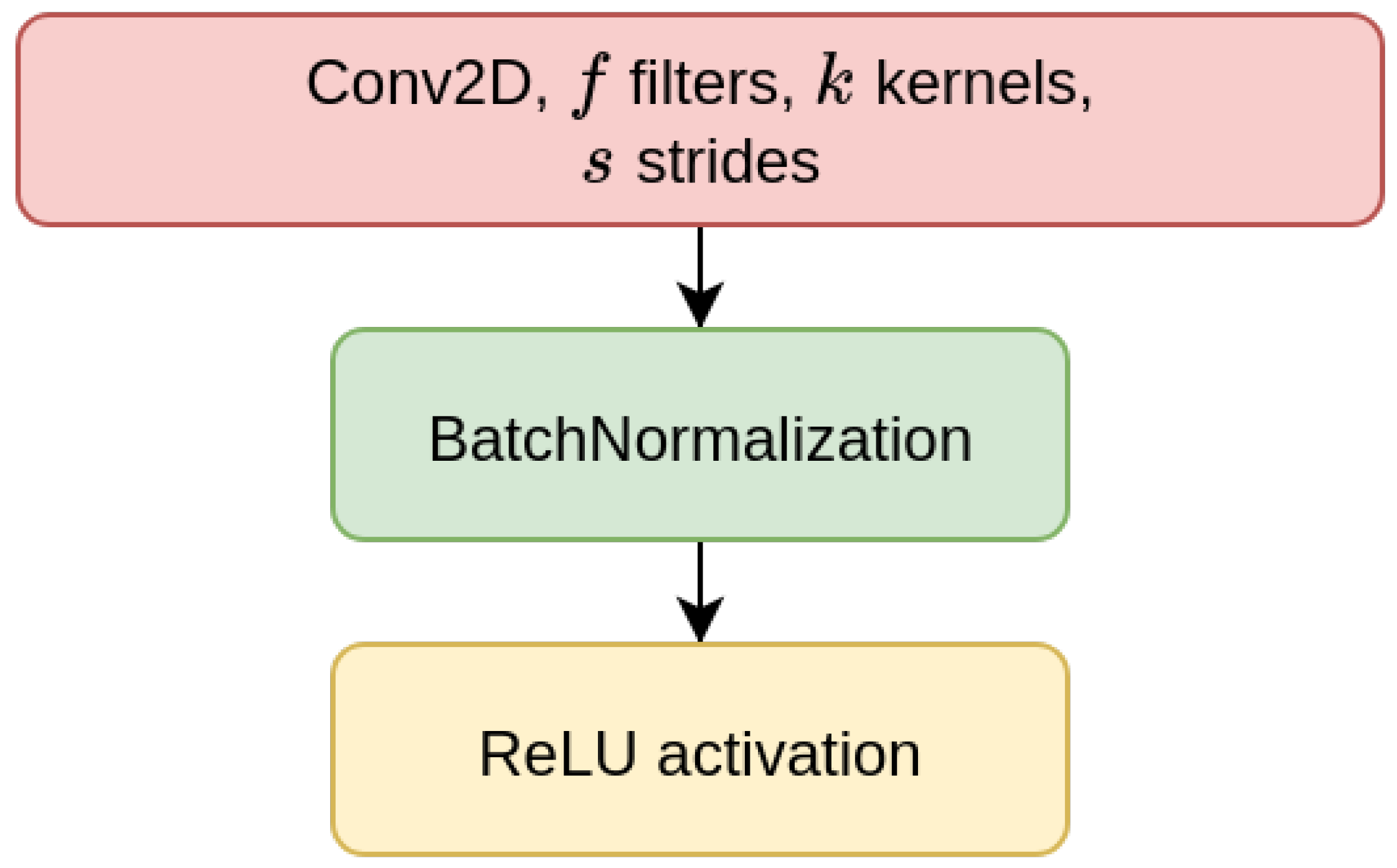
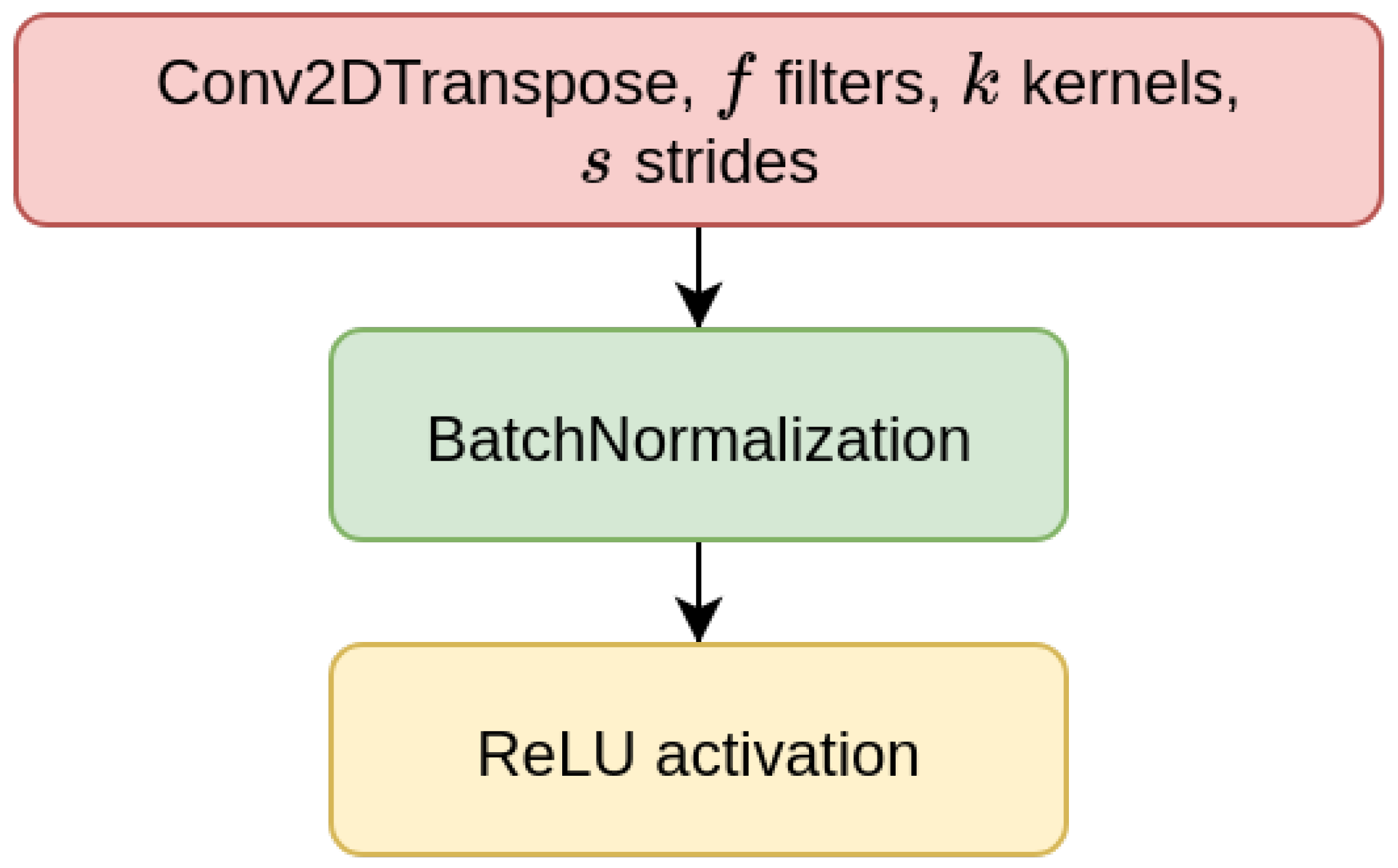
We have considered two types of deep learning models, Contractive Auto-Encoders (CAE) and Convolutional Neural-Networks (CNN), both of which are designed for the task of imputing missing nucleotides in genomic sequences. For each model, we have designed three different architectures which differ for the size of the input sequence they receive as input (either 200, 500, or 1000 nucleotides). This choice is motivated by our will to investigate whether different window sizes bring to different performance. Anyhow, all the models are composed of multiple encoder blocks (EBlock,
Figure 1), and each EBlock is composed by one 2D convolutional layer (Conv2D layer) followed by Batch Normalization and ReLU activation [
69] (as suggested in [
70]). The CAEs also need a decoder sub-module, which is composed of a decoder block (DBlock,
Figure 2), where the Conv2D layer is substituted with a transposed (expanding) Conv2D layer [
71].
All models use Nadam optimizer [
50], with the learning parameters suggested by the authors themselves: learning rate
, decay
and the gradient and momentum coefficients are
and
respectively. The CAE models must reconstruct the input sequences of length N, and their output is therefore structured like the input sequence (i.e.,
nodes, four nodes for each one-hot-encoded nucleotide of the sequence, see
Section 4.1). The output of the CNN is instead composed of four nodes representing only the one-hot-encoding of the missing nucleotide at the center of the input sequence. For this reason, while the input of both models is the same nucleotide sequences containing gaps, the ground truth labels used during training are different. For the CAE models, we compute the loss by using the input sequence without gaps, while the loss of CNNs only considers the prediction of the central gap.
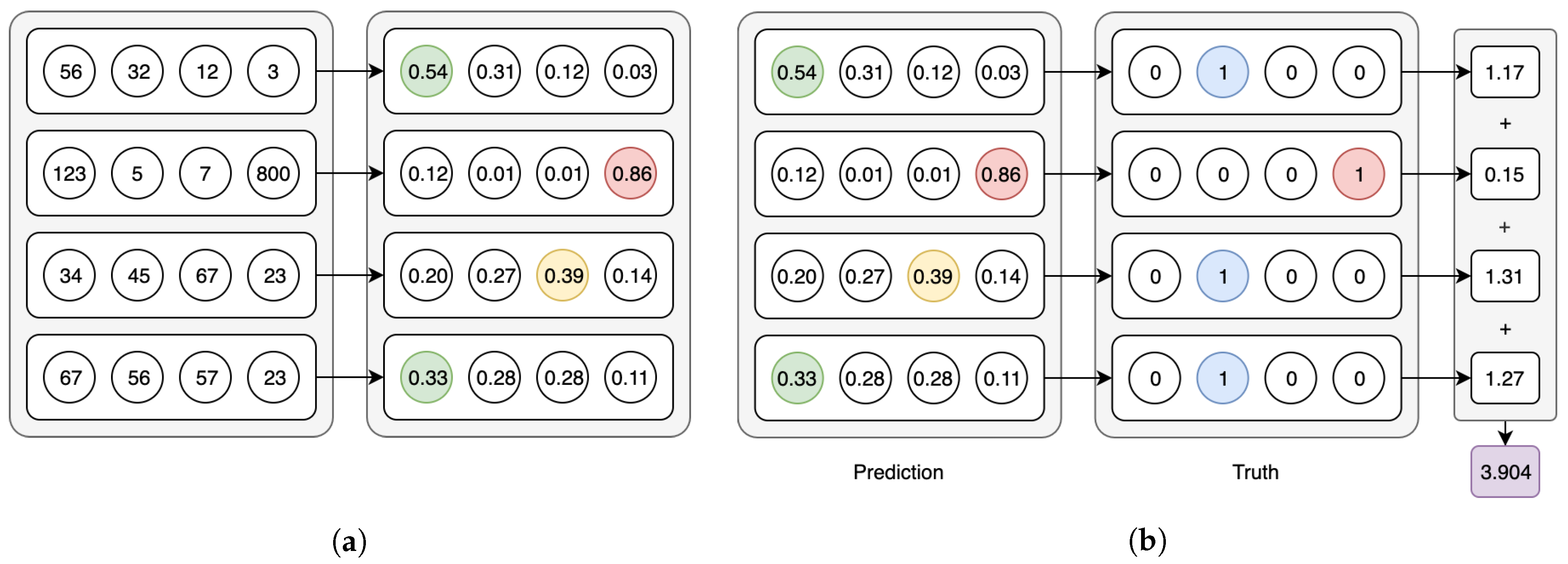
Both model types use the Softmax activation for the last layer and categorical cross-entropy as the loss function—in the CAE models these functions are applied in their per-axis version (
Figure 3a,b). We have used an early-stopping criterion based on the improvement of the validation loss—if no improvement is observed within 10 epochs, the training is interrupted. The maximum possible number of epochs is set to 1000, but we note that using this criterion, no model went over the 100 epochs of training in our experiments. In the following
Section 3.1 and
Section 3.2 we point out the peculiarities of, respectively, the CAE and the CNN models.
3.1. CAE Model
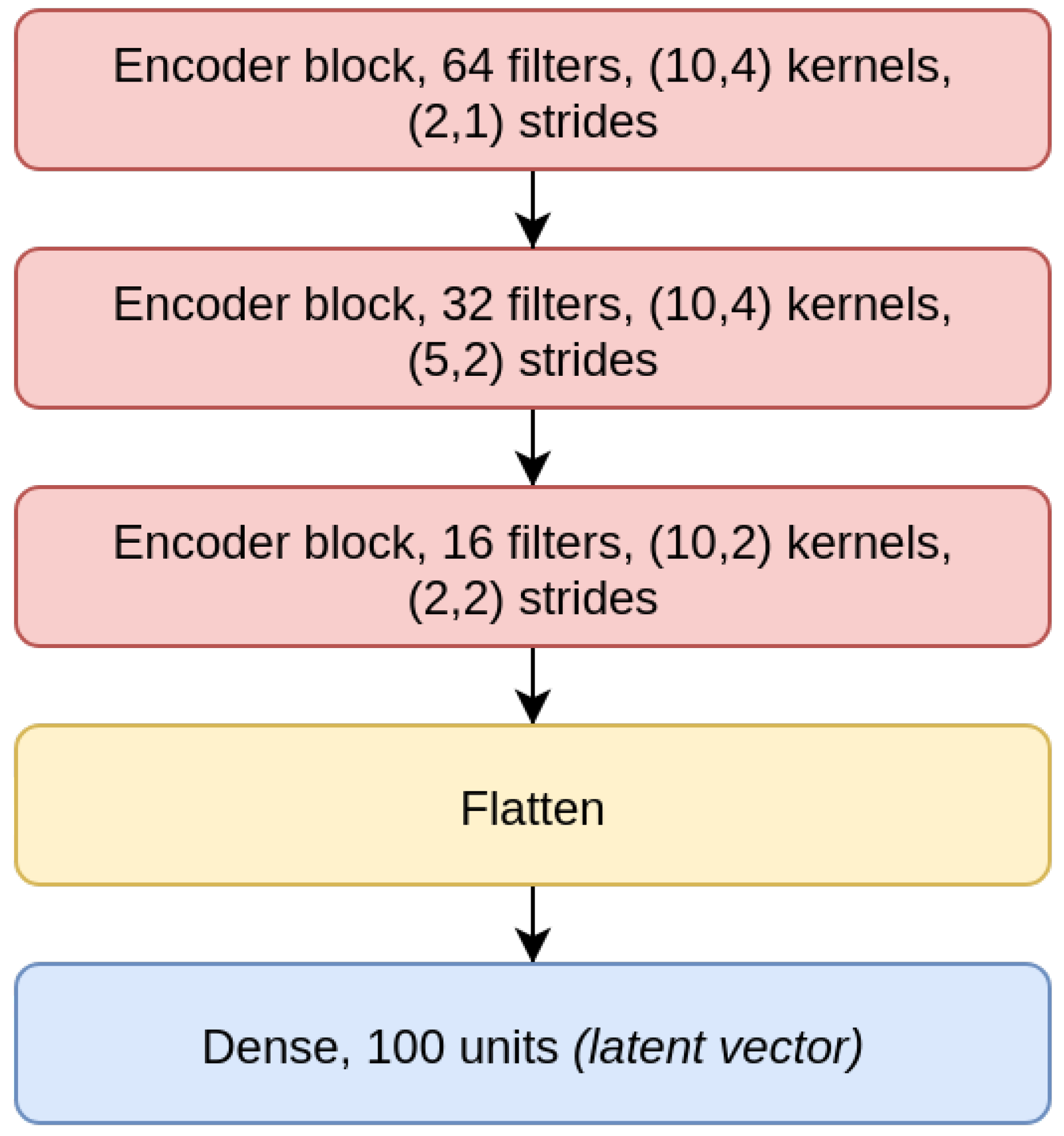
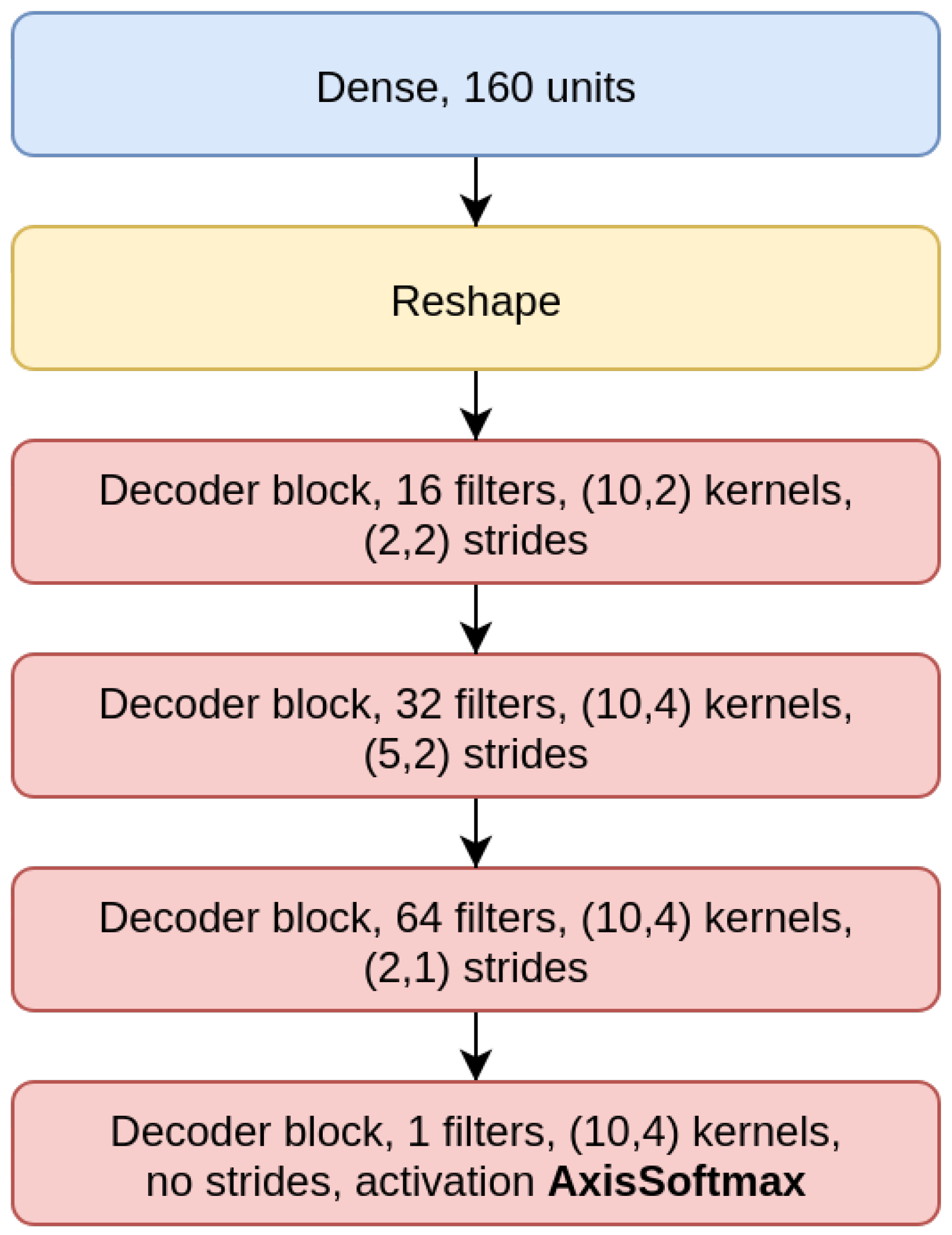
The
CAE model is the concatenation of an encoder (
Figure 4), composed by three EBlocks (
Figure 1), and a decoder (
Figure 5), composed of three DBlocks (
Figure 2). Between the encoder and the decoder parts, the latent layer is a Dense layer with linear activation, whose goal is to embed the data into a latent lower-dimensional vector space. Depending on the considered window size (200, 500, or 1000), the latent layer has a different number of nodes: 100 nodes for the CAE 200, a latent space of size 150 for CAE 500, and 200 neurons for CAE 1000. All the convolutional layers use the padding “same”, which enforces the same output size padding with zeros. The CAE 200, CAE 500, and CAE 1000 structures are detailed in
Table 1.
Note that we use strides instead of max-pooling to reduce the computational load, after considering that the usage of the stride during image recognition tasks on several benchmark datasets [
72] introduces no significant loss of accuracy.
Since the CAE model loss has the same impact on all the output nucleotides, the model might learn an identity function and only reconstruct the known input values without actively imputing the gap at the center of the window, which is the one we aim to fill. In order to prevent this, we weigh differently the loss related to the misclassification of nucleotides, based on their position in the window. Precisely, we set a maximum weight at the window center, where we have the missing nucleotide to be imputed, and we linearly decrease it down to 1 as it reaches the borders. The maximal weights considered are , where the maximal weight that equals 1 produces an unweighted training.
3.2. CNN Model
To focus entirely on the imputation of the missing value at the center of the input sequence, and to avoid altogether the task of also reconstructing the other nucleotides, we have designed CNN models, which may be considered as truncated CAEs that avoid the data reconstruction after its embedding in a lower-dimensional space and therefore need a significantly lower number of parameters, which allows for faster training and inference. Moreover, when viewed as truncated CAEs, CNNs are characterized by a loss that is weighted with an extremely high value, so that only the misclassification of the central nucleotide is considered.
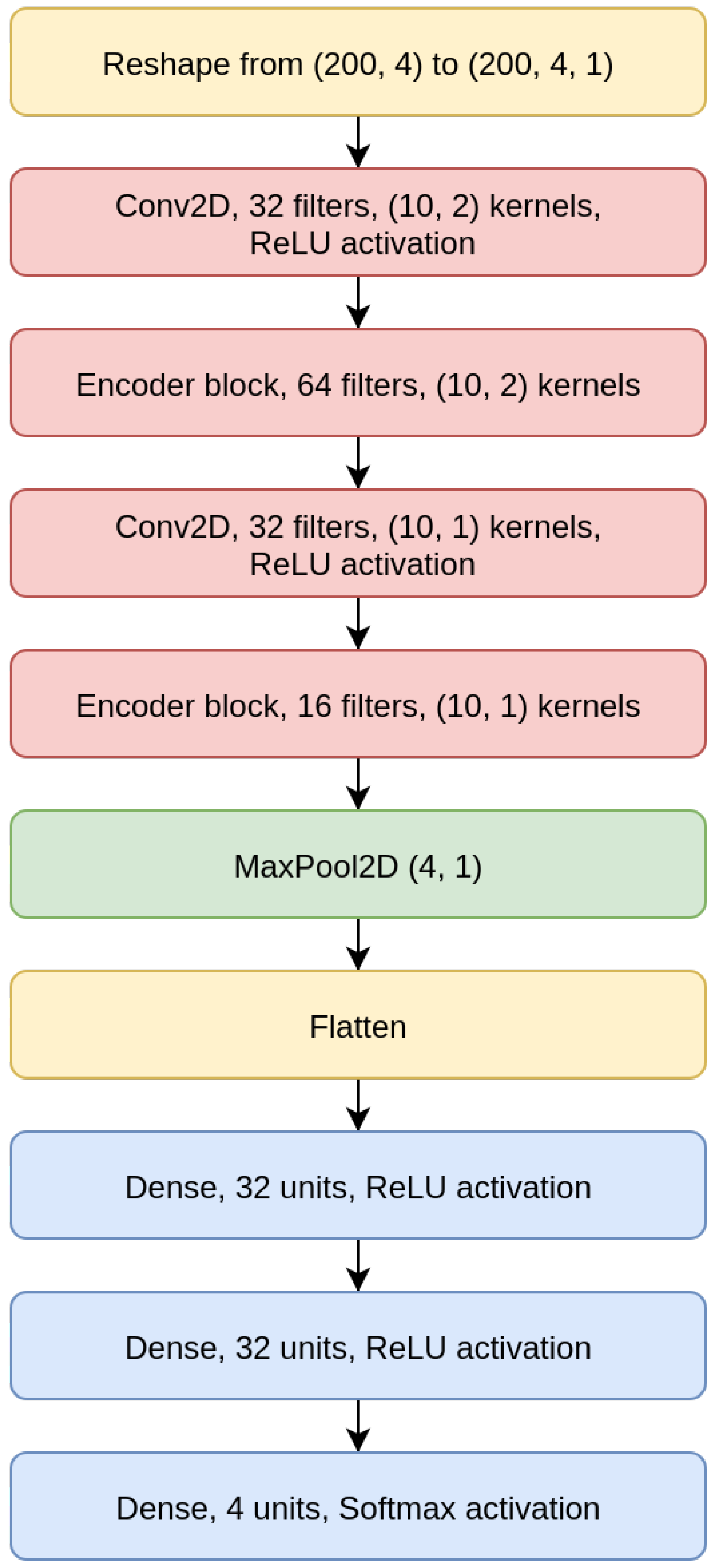
As shown for the CNN 200 model in
Figure 6, the CNNs we designed are composed of two convolutional layers intertwined with EBlocks, followed by a MaxPooling and a Flatten layer (a layer that transforms the bi-dimensional output of a convolutional layer into a one-dimensional vector), and then a sequence of Dense layers on top, which terminates with a Dense layer with four output neurons and Softmax activation.
All CNN models use a categorical cross-entropy as loss, and all convolutional layers use padding. The CNN models structures are detailed in
Table 2.
4. Experimental Setup
We have applied the proposed deep learners for imputing the missing value at the center of a genome sequence which may contain either no-other gaps (single-gap sequence, see
Appendix A.1) or many other gaps (multivariate-gap sequence, see
Appendix A.2). We call this task the
gap-filling task.
Additionally, we considered the ability of the CAE models to reconstruct the whole sequence when the input sequence is either a single-gap sequence or a multivariate-gap sequence. This task, which we call the reconstruction task, should reconstruct the values already present in the input sequence, that is, the known nucleotides, while simultaneously imputing the missing ones, that is, the nucleotides filling the gaps.
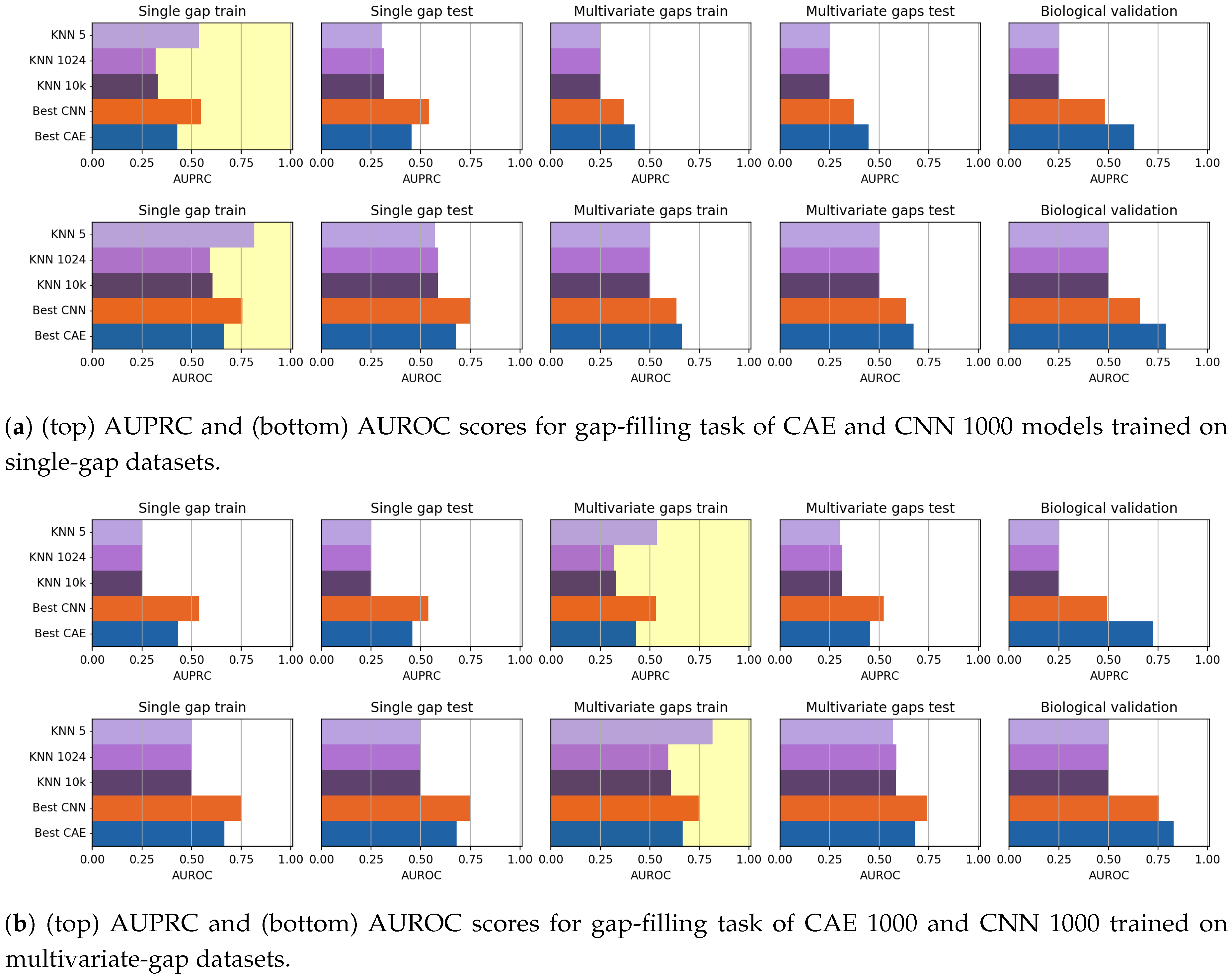
To measure each model performance, we averaged the Categorical Accuracy, the Area Under the Precision Recall Curve (AUPRC) and Area Under the Receiver Operating Characteristic curve (AUROC) scores computed in a one-vs-one fashion (each nucleotide against each other). When evaluating the CAE models on the reconstruction task, all the measures were further averaged over all the nucleotides in the sequence. For each task and each model, we also analyzed the performance on the imputation of each nucleotide, by computing the categorical Accuracy, the AUPRC and AUROC in a one-vs-all fashion, to identify eventual preferential overfitting to one specific nucleotide class. The statistical significance of all the comparisons has been validated by a Wilcoxon signed-rank test [
73] (at the 95% confidence level, that is,
p-value less than
); the Wilcoxon validation has allowed to compare and summarize all the computed performance through Win-Tie-Loss tables (a tie is detected when the Wilcoxon does not detect a significant difference in the compared performance). The same 95% confidence level has also been used for the Pearson correlation tests [
74], and the Spearman correlation tests [
75], which have been used to correlate the achieved performance to the size of the input sequence.
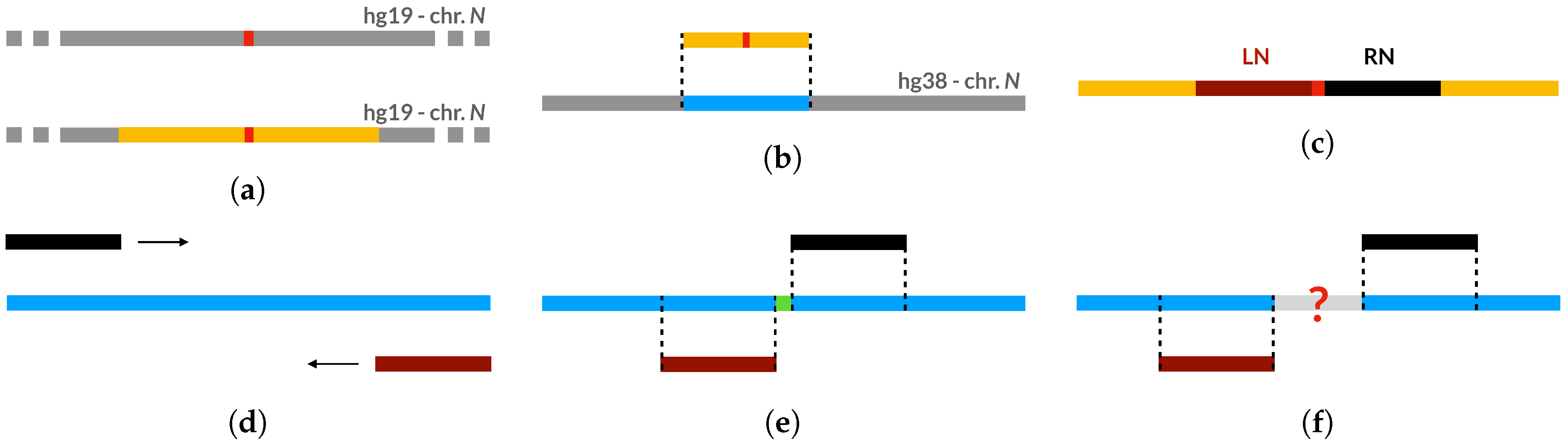
The single-gap, multivariate gap, and biological datasets, which have been used to train, test, and validate our models for both the gap-filling and the reconstruction task, are composed of genome sequences from the reference assembly hg19, the penultimate reference human genome, where we artificially inserted gaps.
As explained in detail in
Appendix A.1 and
Appendix A.2, starting from sequences with no gaps in hg19, we have generated a single-gap dataset (see
Appendix A.1), which contains sequences where only the central nucleotide has been removed, and a multivariate-gap dataset (see
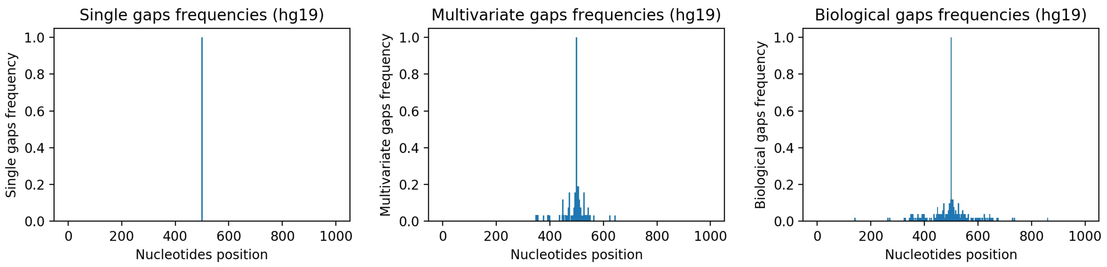
Appendix A.2), which contains the single-gap sequences where many other gaps have been artificially inserted in a way that resembles the biological gaps found in the human genome. To visually assess such similarity,
Figure 7-center and
Figure 7-right show, respectively, the frequencies of the gaps in the multivariate-gap dataset we generated, and the frequency of the gaps in the hg19 sequences we considered for generating the statistical gap model. Moreover, we computed both the Pearson correlation coefficient (0.974,
p-value ≈ 0), as well as the Spearman correlation coefficient (0.998,
p-value ≈ 0) between such frequencies; both coefficients highlight the high correlation between the two signals.
To validate our results, we further composed a biological dataset (
Appendix A.3) which contains the few sequences with single nucleotide gaps in hg19 that were filled in the most recent reference assembly, hg38. The generated single-gap and multivariate-gap datasets have extremely high cardinality, while the biological dataset is considerably smaller (see
Table 3).
4.1. Sequence Data Coding
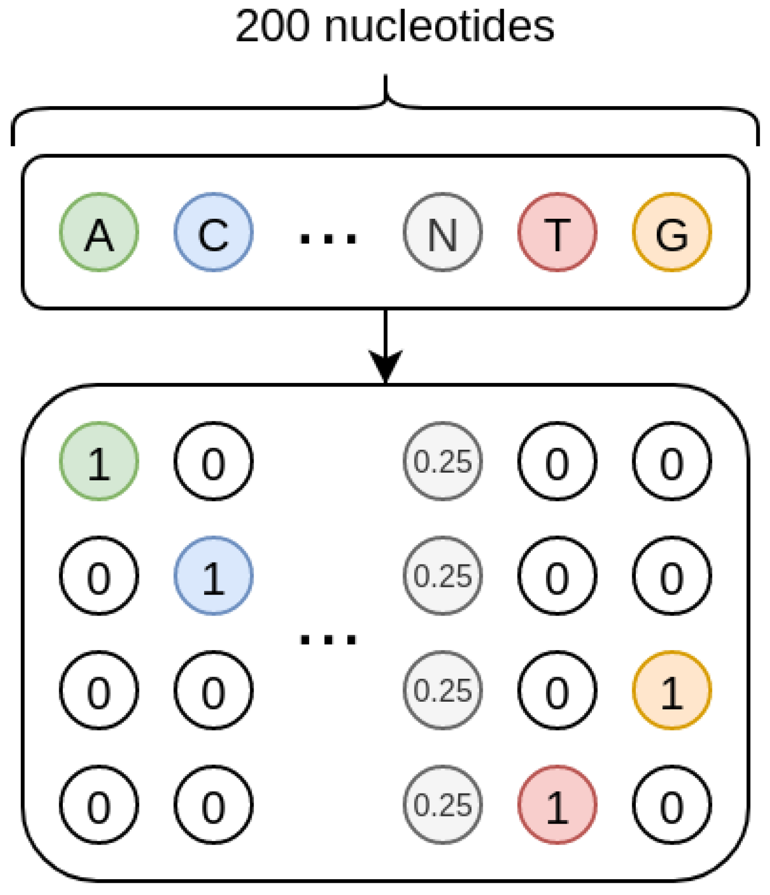
As shown in
Figure 8, the sequences we treat are one-hot encoded, and each missing nucleotide is represented by a 4D vector where all the elements have value 0.25. In such a way, the one-hot encoding procedure inherently encodes a probability. Indeed, when the nucleotide is present, its probability is 1 while that of the other nucleotides is 0; when the nucleotide is missing, the uniform probability distribution is used, so that all the four nucleotides have the same probability.
For the CAE models, this probability setting could be interpreted as a Bayesian framework where the input one-hot encoded sequences would be viewed as the priors, and the model would learn to compute the posteriors by internally modelling the conditional probability that a nucleotide is in a specific position in the sequence given the neighbouring nucleotides.
4.2. Training, Test, and Validation Partitions
While the sequences in the biological dataset are only used for validating the models, the single-gap and multivariate-gap sequences are used for training and testing. For this reason, we have split the available sequences into train and test set by using a randomly generated chromosomal holdout to avoid positional bias caused by samples from the same chromosome.
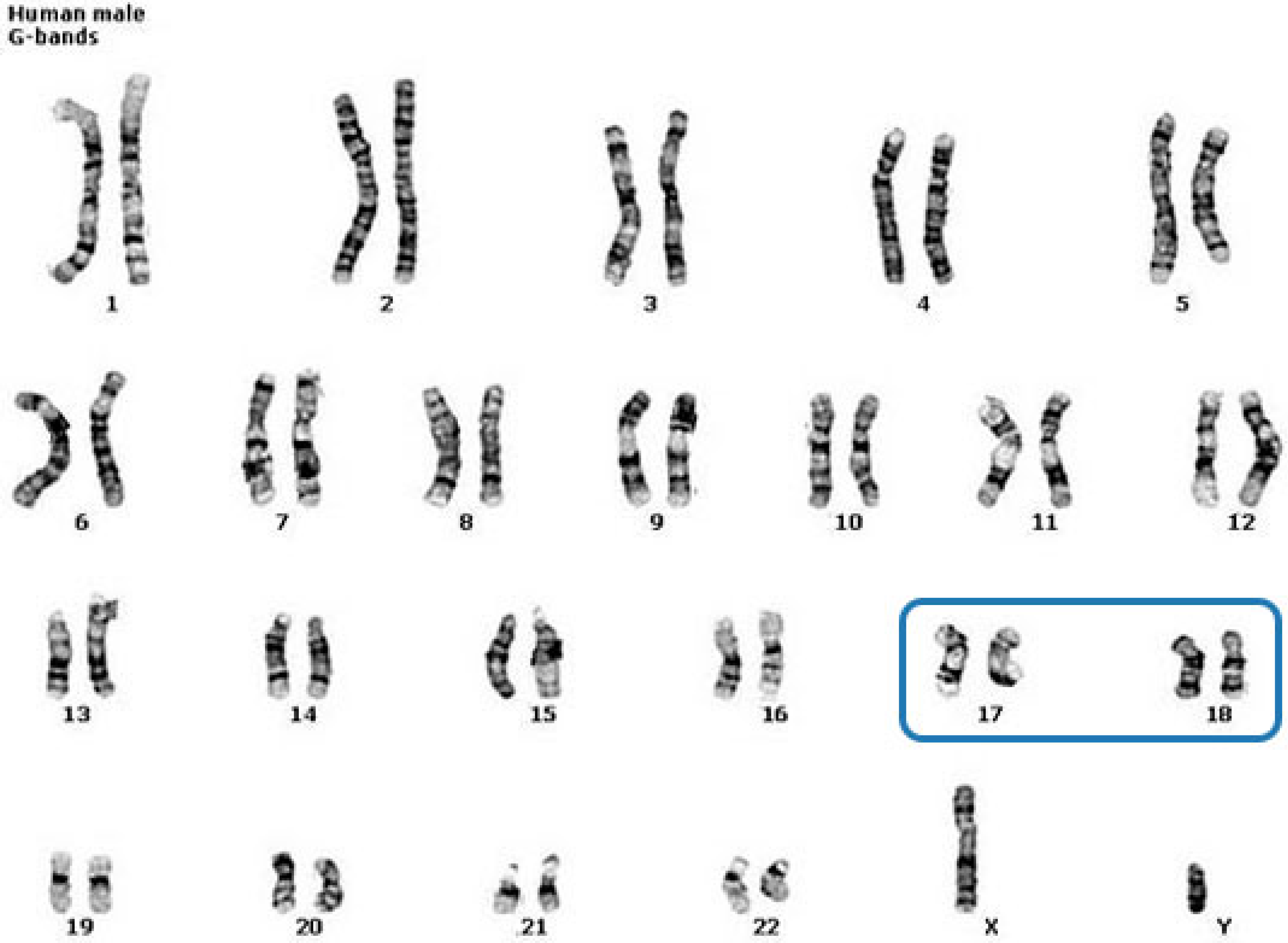
Precisely, we have randomly selected 17 and 18 chromosomes for testing, and we have used the other chromosomes for training (
Figure 9). Both train and test partitions contain a considerable amount of sequences (
Table 3). The test-train cardinality proportion is ≈17.97%. As detailed in
Table 3, when comparing the number of gaps corresponding to each of the four nucleotides, the train and test sets from the single-gap and multivariate-gap datasets are only slightly unbalanced, while the biological dataset contains highly unbalanced proportions of missing nucleotides.
Since, for each model, we also wanted to assess the model robustness with respect to the number of gaps viewed during training, we evaluated two instances for each model. The first instance is obtained by training the model on the training sequences with only one gap at the center (single-gap training set); this instance is evaluated on a validation set composed by all the other unseen (single-gap and multivariate-gap) sequences, independently on the number of gaps (that is, this instance is tested both on sequences in the single-gap test set, and on all the sequences with more than one gap, and belonging to the multivariate train and test sets). Similarly, the second instance of the model is trained by using the sequences with many gaps in the multivariate-gap training dataset, and is tested on the validation set composed by all the other not-seen sequences (single-gap train and test sequences plus multivariate-gap test sequences). Of course, the two instances are also tested on all the sequences in the biological dataset.
In this way, for each instance of the model, we obtain five evaluations (shown separately in the next
Section 5): the evaluation on the set used for training, which provides a first evaluation of the model generalization or overfitting, the evaluation of the results obtained on all the three sets in the validation set, and the assessment on the biological dataset.
All the data generation code and the deep models are available for research purposes at
the public repository on GitHub (
https://github.com/LucaCappelletti94/repairing_genomic_gaps). All the deep models have been implemented using Keras/TensorFlow [
76,
77] and the trained models are available in the GitHub repository. Note that all the code has been optimized in order to reduce both the memory requirements as well as the computational time so that the experiments may run on consumer-grade computers equipped with a GPU.
6. Discussions, Conclusions and Future Works
In this paper, we have investigated the usage of CAEs and CNN for the task of missing data imputation in complex datasets. The proposed deep-learning imputation methods have been successfully applied on genome datasets for filling the missing nucleotides (gap-filling task) or for reconstructing entire genome sequences while simultaneously filling their gaps (reconstruction task). Our experiments have shown that both CAEs and CNNs outperform KNN-imputation, a widely used state-of-the-art technique.
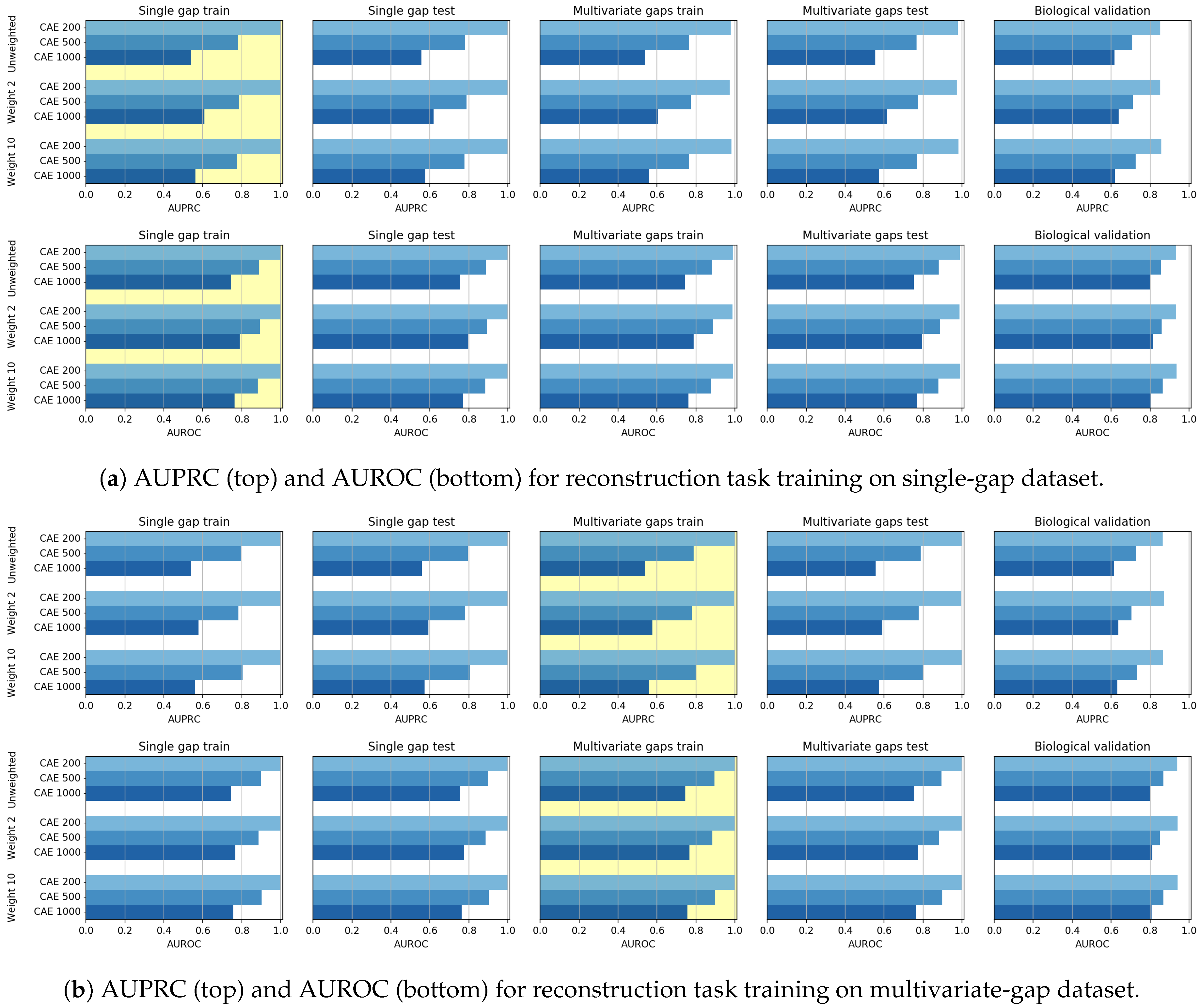
Precisely, the promising results achieved by the CAEs suggest that the lower-dimensional representation expressed in the latent space retains all the salient information required for describing the structure of the input sequence, as it is needed in this case study. For this reason, our future works will be aimed at applying the CAES for supporting classification tasks. Precisely, by training the CAEs for a specific classification task, we could obtain more discriminative representations in the latent space, which could be used as input to other discriminating algorithms [
85,
86].
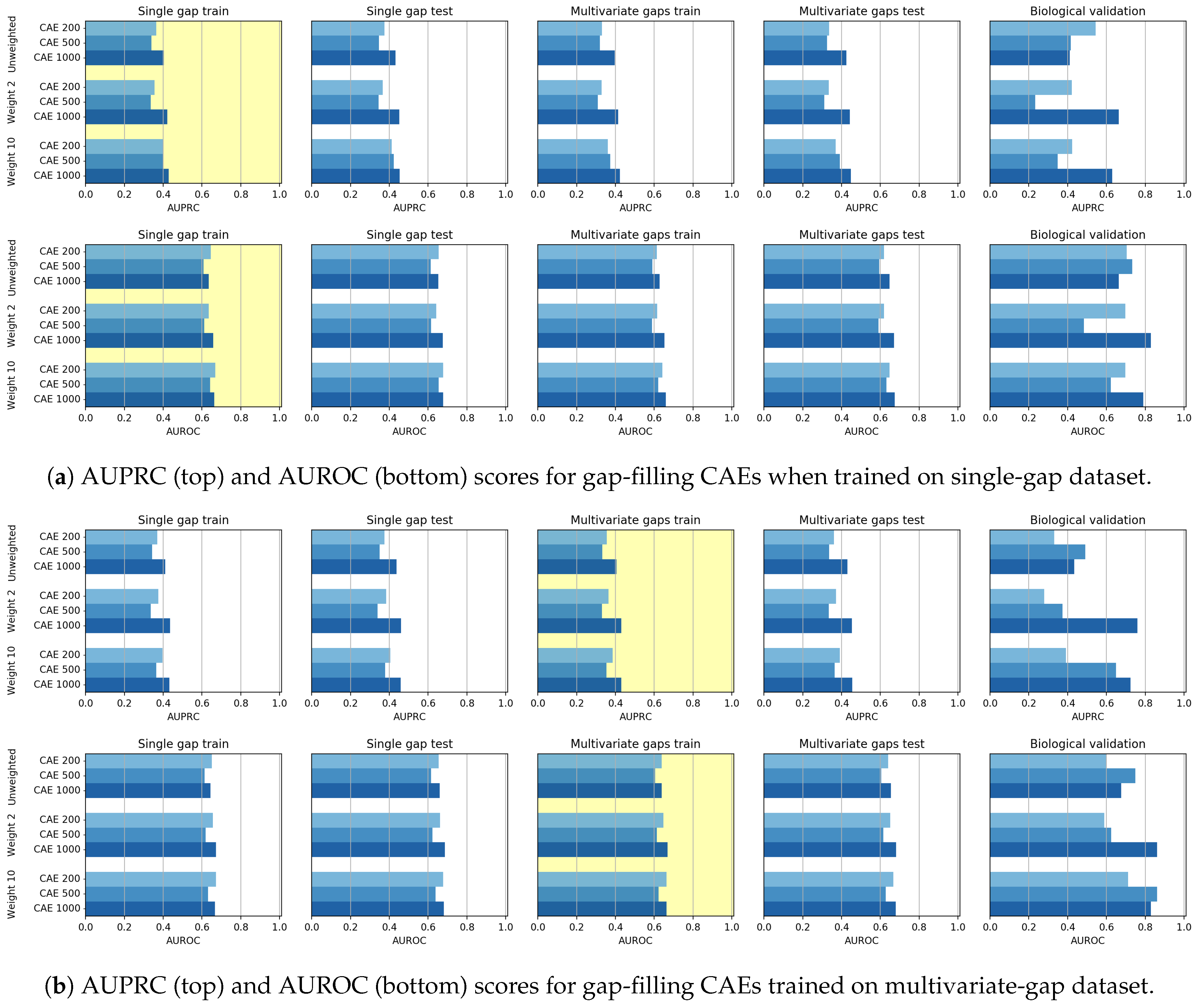
Though the CAE models obtained promising reconstruction results, after experimenting their gap-filling capability we experienced poorer results when compared to CNNs, probably meaning that the network learning ability is dispersed with the aim of producing a good reconstruction of the whole sequence. We, however, noted that when the size of the input sequence increases, the CAE performance increases. Moreover, for what regards the gap-filling task, our proposal of weighing the central nucleotide differently is promising since it allows increasing the gap-filling performance.
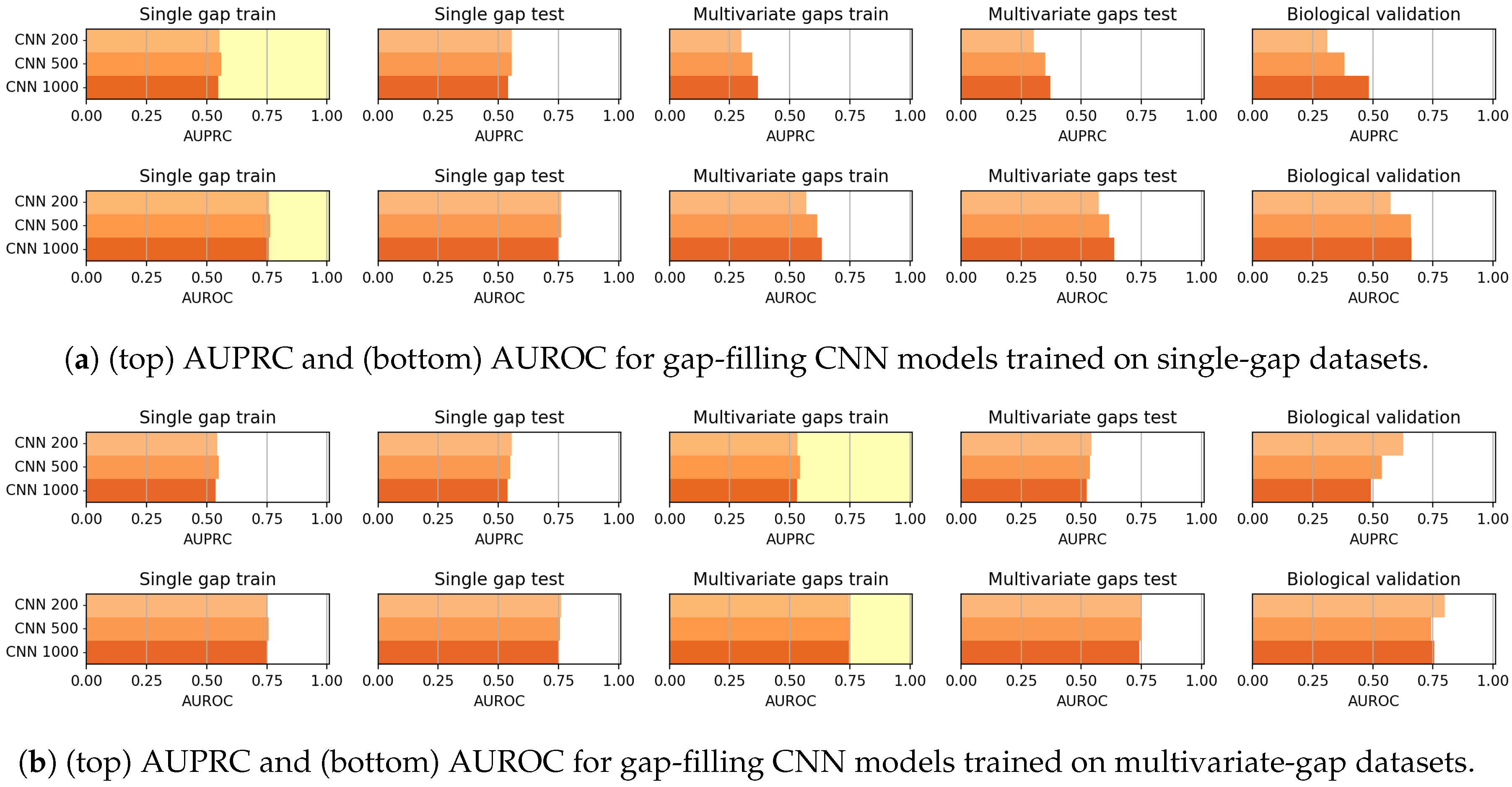
As mentioned before, the CNN models generally outperformed the CAE models in the gap-filling task. On the other hand, the validation of the Biological dataset shows that CAE is competitive with CNN, but the reduced cardinality of the dataset suggests particular caution in drawing conclusions.
Anyhow, both models achieved promising results which we believe are robust with respect to the parameters settings.
Indeed, the only evident critical parameter we introduced in this work, is the weight of the AE, which allows weighing more the imputation performance of the missing element. To test the criticality of the weight setting, we have shown experiments where completely different weight values are used. The reported results show that, indeed, the AE should give more importance to the reconstruction of the element that must be imputed. Therefore, by observing the achieved results it is easy to set the best weight value.
The other parameters that may influence the achieved performance, are those related to the training algorithm (Nadam optimizer [
50]). Regarding their choice, we used the settings proposed by the Nadam author themselves. The author’s parameter setting was a two-fold decision—he chose the parameter setting allowing to achieve a good stable performance (negligible performance variations are visible when the parameter values are varied in the neighborhood of the chosen values).
Anyhow, the promising results obtained by both the models, and our awareness that the stability of our performance with respect to the parameter setting could not be valid for the specific problem being tackled, motivate our future works aimed at further improving performance by searching for the best hyperparameter settings in a wider hyper-parameter space. Parameter search may be performed by random search [
51], or Bayesian optimization [
52], which have proven to effectively find an optimal setting [
48].
Anyhow, considering both the CAEs and CNN results, auto-encoder models seem to provide useful and informative data embedding, while the CNN models could seem promising gap-filler. Natural future work could, therefore, be aimed at integrating U-Nets auto-encoders and CNNs, optimized through bayesian search, to obtain a novel structure exploiting the strengths of both the architectures.
Eventually, we could even modify the deep convolutional architecture, by substituting it with a Recurrent Neural Network [
87].
Finally, we note that the gap filling application presented in this paper is a Proof of Concept, to show how deep imputers may be successfully applied to solve the problem of the complex-data imputation. In this case, the architecture of the proposed techniques has been designed to adhere to the chosen complex categorical data. For this reason, the presented deep learner process a 2D binary (one-hot-encoded) input and are constituted of internal layers using 2D convolutional filters, which are the most appropriate for this problem, and an output layer with one node for each category. After opportunely diminishing/augmenting the number columns in the input layer and the number of nodes in the output one, the presented techniques could be retrained to fill the gap of any other type of complex categorical dataset, where convolutional filtering is appropriate. Note that when convolutional filters are not appropriate, dense layers could be used.
On the other hand, if (2D or 1D) continuous complex data should be imputed, both the input layers, and the internal filters should be adapted to the input dimension (1D convolutional filters or 1D dense layers for 1D input, and 2D filters or 2D dense layers for 2D input), while the multi-node output should be substituted by a unique node containing the value of the missing element. Of course, in this case, the same training procedure would result in a regressor rather than in a classifying machine (since the predicted categorical data would be substituted by a continuous value). Our future works will be aimed at testing the deep imputers for application where continuous complex data (e.g., epigenomic data) must be imputed.

 ,
, 


