Structured (De)composable Representations Trained with Neural Networks †


Departement Computerwetenschappen, Celestijnenlaan 200a—bus 2402, 3001 Leuven, Belgium
*
Author to whom correspondence should be addressed.
†
This paper is an extended version of our paper published in the 9th IAPR Workshop on Artificial Neural Networks in Pattern Recognition, ANNPR 2020, Winterthur, Switzerland, 2–4 September 2020.
Computers 2020, 9(4), 79; https://0-doi-org.brum.beds.ac.uk/10.3390/computers9040079
Submission received: 14 September 2020
/
Revised: 28 September 2020
/
Accepted: 29 September 2020
/
Published: 2 October 2020
(This article belongs to the Special Issue Artificial Neural Networks in Pattern Recognition)
Abstract
:This paper proposes a novel technique for representing templates and instances of concept classes. A template representation refers to the generic representation that captures the characteristics of an entire class. The proposed technique uses end-to-end deep learning to learn structured and composable representations from input images and discrete labels. The obtained representations are based on distance estimates between the distributions given by the class label and those given by contextual information, which are modeled as environments. We prove that the representations have a clear structure allowing decomposing the representation into factors that represent classes and environments. We evaluate our novel technique on classification and retrieval tasks involving different modalities (visual and language data). In various experiments, we show how the representations can be compressed and how different hyperparameters impact performance.
1. Introduction
We propose a novel technique for representing templates and instances of concept classes that is agnostic with regard to the underlying deep learning model. Starting from raw input images, representations are learned in a classification task where the cross-entropy classification layer is replaced by a fully connected layer that is used to estimate a bounded approximation of the distance between each class distribution and a set of contextual distributions that we call “environments”. By defining randomized environments, the goal is to capture common sense knowledge about how classes relate to a range of differentiating contexts and to increase the probability of encountering distinctive diagnostic features. This mechanism loosely resembles the associative nature of human memory. Long-term memory storage is believed to rely on semantic encoding that performs better if it can be associated with existing contextual knowledge [1]. Additionally, relating classes to arbitrarily chosen environments increases the probability of encountering distinctive diagnostic features, which should help retrieval, as might be the case with human long-term memory [2]. A recent theory named “The Thousand Brains Theory of Intelligence” [3] suggests that multiple parts of the neocortex learn complete models of objects with respect to different reference frames. The approach in this paper resembles these mechanisms. Our experiments confirm the value of such an approach.
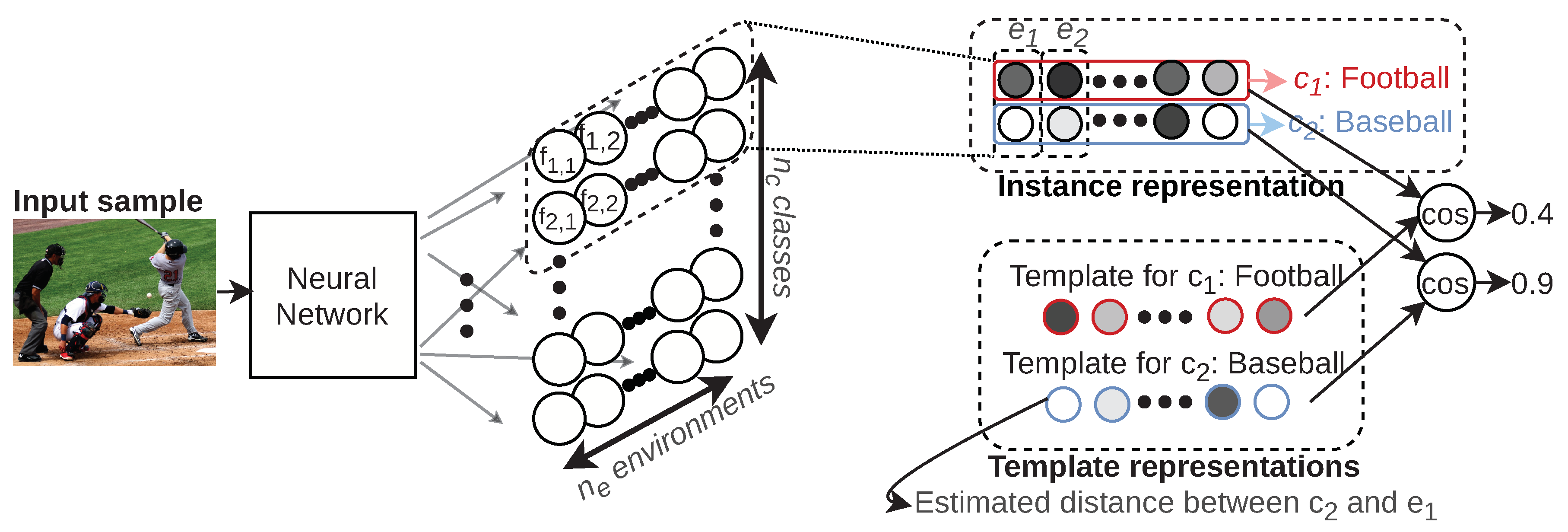
In this paper, classes correspond to (visual) object labels, and environments correspond to combinations of contextual labels given by either object labels or image caption keywords. Representations for individual inputs, which we call “instance representations”, form a 2D matrix with rows corresponding to classes and columns corresponding to environments, where each element is an indication of how much the instance resembles the corresponding class versus the environment. The parameters for each environment are defined once at the start by uniformly selecting a randomly chosen number of labels from the power set of all available contextual labels. The class representation, which we refer to as the “template”, has the form of a template vector. It contains the average distance estimates between the distribution of a class and the distributions of the respective environments. By computing the cosine similarity between the instance representation and all templates, class membership can be determined efficiently.
To get a better understanding of the setup, Figure 1 provides an example. For an input image showing a scene from a baseball game, a neural network learns a projection to a 2D representation. The amount of rows corresponds to the amount of classes and the amount of columns to the amount of environments. In this example, the first row corresponds to the label “Football”, and the second row corresponds to the label “Baseball”. Each of the environments , , … consists of a set of randomly selected labels; for example, could be constructed with the labels “Bat” and “Basketball”. The instance representation then gives an indication of how this image relates to these environments for each of the classes. The template representations give the average distance estimate between class and environments. For example, for the class (i.e., “Baseball”), the template would show a small distance with respect to as the notions “Baseball” and “Bat” are closely related. By comparing the values of the instance representation with the template representations, one can find that the second row of the instance representation (corresponding to “Baseball”) is highly similar to the template representation for “Baseball”. At the same time, the first row of the instance representation (corresponding to “Football”) is not that similar to the template representation for “Football”.
Template and instance representations are interpretable as they have a fixed structure comprised of distance estimates. This structure is reminiscent of traditional language processing matrix representations and enables operations that operate along matrix dimensions. We demonstrate this with a Singular Value Decomposition (SVD), which yields components that determine the values along the rows (classes) and columns (environments), respectively. Those components can then be altered to modify the information content, upon which a new representation can be reconstructed. The proposed representations are evaluated in several settings:
- Multi-label image classification, i.e., object recognition with multiple objects per image;
- Image retrieval where we query images that look like existing images, but contain altered class labels;
- Single-label image classification on pre-trained instance representations for a previously unseen label;
- Rank estimation with regard to the compression of the representations;
- Hyperparameter selection and the influence on classification performance and sensitivity;
- The effect of environment composition on classification performance: we show that models that are trained with more environments and with a suitable diversity in environment composition lead to more informative features in the penultimate layer.
Finally, given the novelty of this approach, we will suggest several promising research directions for future work.
Contributions: (1) We propose a new deep learning technique to create structured representations from images, entity classes, and their contextual information (environments) based on distance estimates. (2) This leads to template representations that generalize well, as successfully evaluated in a classification task. (3) The obtained representations are interpretable as distances between a class and its environment. They are composable in the sense that they can be modified to reflect different class memberships as shown in a retrieval task.
2. Background and Related Work
We briefly discuss the useful background related to different aspects of our research and investigate related works.
2.1. Representing Entities with Respect to Context
Traditionally, natural language processing has relied extensively on discrete representations. The presence of a word or phrase in a sentence might be indicated by a one or zero (BOW [4]). A slightly more sophisticated, but widely used version is TF-IDF [5], which takes into account the frequency of words. This leads to very sparse representations with the undesirable quality that two sentences that have a similar meaning can be orthogonal in terms of representations. To combat these issues, neural networks mostly rely on dense, continuous-valued representations. Such representations are often built in an unsupervised manner by extracting the meaning from the surrounding context. This is the case for Word2Vec [6] word representations, as well as representations from more recent language models such as ELMo [7] and BERT [8]. A downside of such representations is that they lose access to the discrete input symbols and have no direct manner to interpret or manipulate the meaning that is distributed among the dimensions.
A pragmatic method to represent a collection of documents is by using structured matrices, e.g., by creating document-term matrices where rows are documents and columns are terms. Such matrices can be decomposed with SVD or non-negative matrix factorization. Low-rank approximations are found with methods like latent semantic indexing [9]. This typically solves the higher mentioned orthogonality and interpretability issues by finding meaningful dimensions regardless of the vocabulary that was used in the document. Some typical applications are clustering, classification, retrieval, etc. A significant benefit of such structured representations is that outcomes can usually be interpreted with respect to the contextual information. For example, when clustering textual documents, one can visually inspect to what extent particular terms contribute to each cluster. Contrary to our work, earlier methods built representations purely from labels and did not take deep neural network-based features into account.
Other methods have recently also attempted to use co-occurrence information to represent information within richer contexts. Singh et al. [10], for example, created an unsupervised sentence representation where each entity is a probability distribution based on co-occurrence of words.
2.2. Distances to Represent Features
A distinction can be made between machine learning problems that compute metrics between individual instances (for example, by means of the Euclidean distance) and those that compare subsets in large datasets. For the latter type of problems, a recent series of works has explored the use of the “Optimal Transport Problem” (OTP) [11]. The distance that is found by solving the OTP between two distributions is called the Earth Mover’s Distance (EMD) [12], also known as the Wasserstein distance. Whereas the OTP is traditionally solved via some variation of Sinkhorn iterations [13,14], neural network-based approximations of the EMD have been widely used in recent years [15,16,17], mostly in relation to generative adversarial networks [18].
The EMD has been applied to several natural language processing applications recently. The Word Mover’s Distance (WMD) [19], for example, measures the distance between text documents. The WMD thus gives the minimal amount of effort to move Word2Vec-based word embeddings from one document to another. The authors used a matrix representation that expresses the distance between words in respective documents. They noted that the structure is interpretable and that it performs well on text-based classification tasks. Singh et al. [10] embedded documents by learning Wasserstein distances between contexts. Wasserstein distances have also been used to maximize distances between classes while minimizing intra-class discrepancy for feature learning in Wasserstein discriminant analysis [20].
2.3. Random Features
Many modern machine learning applications act on data that have very high dimensionality. A popular method to make tasks more tractable is to first project the data to a lower dimensional space. Computing a suitable projection can however be computation and resource expensive.
The Johnson–Lindenstrauss (JL) lemma [21] has been a central result in this regard, stating that a point cloud can be mapped with a random Lipschitz projection to a lower dimensional space in which intra-point distances are preserved with high probability. Preserving the original structure of the point cloud is highly desirable as some operations can be performed more easily in the lower dimensional space. This principle has been applied on sparse data in “compressed sensing” [22,23] applications, with the additional constraint that the data can be transformed back to the original space.
Similarly, the work by Rahimi and Recht [24] showed that random projections to a low-dimensional feature space allow fast computations with linear methods for the training of kernel machines. This idea was further developed by Wu et al. [25], who created the word mover’s embedding, an unsupervised feature representation for documents. This embedding is obtained with a kernel that employs a mapping to a lower dimensional space with the word mover’s distance [19]. The feature space is infinitely large where feature dimensions consist of random documents that are created by sampling a set of random words. One can then approximate the distance between two documents by comparing how they relate to the random documents. As we will show in Section 3.6, our work follows a similar line of thought, but in an end-to-end deep neural network setting with (potentially) multiple modalities.
2.4. Interpretable Neural Networks
Many works that attempt to increase interpretability in neural networks focus on methods to visualize features or neurons [26,27]. Other approaches focus on attribution, for example with attention mechanisms [28]. It is then possible to investigate which elements contributed to an outcome, but this does not explain satisfactorily why and how a decision was made. To this effect, it would be more useful to obtain compositionality: understanding how different components interact and can be combined leads to increased understanding. This can be achieved by imposing more structure to networks. A typical approach is to aim for disentangled representations, usually performed with (variational) autoencoders [29,30]. That said, the structure that is obtained from disentanglement is not immediately useful for further compositions. By mapping instances to a 2D representation, we show that we obtain a structure that can be used for compositionality (see Section 3.5).
In summary, our work borrows from each of the aspects we mentioned above. We create representations that characterize entities with respect to different contexts while exploiting the structure for compositionality. We use a distribution-based distance metric to create contextual features. As inspired by the word mover’s embeddings, representations consist of feature maps with respect to random dimensions. Our work most importantly differs from previous work in the following manners: (1) we use end-to-end deep neural network training to include rich image features when building representations; (2) information from different modalities (visual and language) can be combined.
3. CoDiR: Method
In this section, we discuss the methodology to define environments and their usage in instance and template representations. We will also show how to perform the neural network training and how to exploit the structure of the representations for composition. We refer to our method as Composable Distance-based Representation learning (CoDiR). We end this section by exploring the connection to random feature maps.
3.1. Setting Up Environments
Concretely, in this work, we deal with image instances x that are distributed according to . Images have non-exclusive class labels , which in this work are visual object labels (e.g., dog, ball, …). Image instances x are fed through a (convolutional) neural network N. The outputs of N will serve to build representations with rows and columns, where indicates the amount of environments. Each environment will be defined with the use of discrete environment labels , for which we experiment with two types: (1) the same visual object labels as used for the class labels (such that ) and (2) image caption keywords from the set of the most common nouns, adjectives, or verbs in the sentence descriptions in the dataset. We will refer to the first as “CoDiR (class)” and the latter as “CoDiR (capt )”.
Two types of representations will be created: (1) templates that are generic class representations and (2) instance representations . Each element of is a distance estimate between distributions and , where is shorthand for . Informally, is the joint distribution modeling the data distribution and class membership . To obtain , several steps are performed before training:
- Hyperparameter is set, giving the amount of environments.
- Hyperparameter R is set, giving the maximum amount of labels per environment.
- For the j-th environment, we then:
- (a)
- Sample the actual amount of labels ;
- (b)
- Sample the labels , with , uniformly without replacement from the set of all discrete environment labels .
Now, , the set of images for environment , is given by with the set of images with label . Thus, similarly to , we have . Note that by sampling a random amount of labels per environment, as inspired by [25], we ensure diversity in the type of composition of environments, with some holding many labels and some few. In Table 1, we summarize the most important notations.
Example 1.
To clarify the creation of environments before the training phase, we provide a short, simple example. Assume we have a set of class labels: {dog, cat, ball, baseball, …} For this example, we will use these class labels to construct environments. As a first step, we set the hyperparameters and , i.e., we will create two environments with a maximum of five labels in each. Now, for both environments, we will sample the amount of labels and the labels themselves:
- For the first environment, we sample . Thus, we need to sample one label from {dog, cat, ball, baseball, …} : “ball”.
- Similarly, for the second environment, we sample . Thus, we need to sample two labels from {dog, cat, ball, baseball, …} : “dog”, and “ball”.
In Section 4.7.1, the selection of hyperparameters and R is examined further. In the following section, we discuss how to obtain distance estimates between the distributions of classes and environments.
3.2. Contextual Distance
We propose to represent each image as a 2D feature map that relates distributions of classes to environments. A suitable metric should be able to deal with neural network training, as well as potentially overlapping distributions. A natural candidate is a Wasserstein-based distance function [15]. A key advantage is that the critic can be encouraged to maximize the distance between two distributions, whereas metrics based on Kullback–Leibler (KL) divergence are not well defined if the distributions have a negligible intersection [15]. In comparison to other neural network-based distance metrics, the Fisher Integral Probability Metric (Fisher IPM) provides particularly stable estimates and has the advantage that any neural network can be used as f as long as the last layer is a linear, dense layer [31]. The Fisher IPM formulation bounds , the set of measurable, symmetric and bounded real valued functions, by defining a data dependent constraint on its second order moments. The IPM is given by:
In practice, the Fisher IPM is estimated with neural network training where the numerator in Equation (1) is maximized while the denominator is expressed as a constraint, enforced with a Lagrange multiplier. While the Fisher IPM is an estimate of the chi-squared distance, the numerator can be viewed as a bounded estimate of the inter-class distance, closely related to the Wasserstein distance [31]. From now on, we denote this approximation of the inter-class distance as the “distance”. During our training, critics are trained from input images to maximize the Fisher IPM for distributions and , . The numerator then gives the distance between and . We denote , with , i.e., the evaluation of the estimated distances over the training set. Intuitively, one can see why a matrix with co-occurrence data contains useful information. A subset of images containing “cats”, for example, will more closely resemble a subset containing “dogs” and “fur” than one containing “forks” and “tables”.
3.3. Template and Instance Representations
Generic class representations can then simply be obtained from the rows of as they contain the average distance estimates of a class with respect to all environments. We thus define to be the template representation of class . Concretely, each element gives an average distance estimate for how a class relates to environment , where smaller values indicate that the class and environment are similar or even (partially) overlap. For the instance representation for an input s, we then propose to use with elements given by Equation (2):
where is simply the output of critic for the instance s. The result is that for an input s with class label , is correlated to as its distance estimates with respect to all different environments should be similar. Therefore, the inner product between vector and the template will be large for input instances from class i, and small otherwise.
In general, the inner product of the obtained feature maps can be used to compute similarity between two instances with respect to a class. For a given class and input images x and y, this would become:
In this work, we concretely use the cosine similarity as the similarity measure. To express class membership, we use a shorthand notation , and otherwise. As templates indicate the average distance between classes and environments, we thus evaluate class membership as follows:
with a threshold (the level of which is determined during training), and cos is the cosine similarity. As classes can be evaluated separately, such templates can be evaluated, for example in multi-label classification tasks (see Section 4). Finding the classes for an image is then simply calculated by computing whether , .
3.4. Implementation
To obtain and , it is then necessary to train critic networks. This is of course not feasible in practice. For our approach, we therefore use a common neural network where the last layer (e.g., the classification layer) is replaced by a single layer, fully connected neural network with output size . The outputs of this network give with and (see Figure 1).
During training, any given mini-batch will contain inputs with many different and . To maximize Equation (1) efficiently, instead of feeding a separate batch for the instances of and , we use the same mini-batch. Additionally, instead of directly sampling , we multiply each output with a mask where . Here, stands for the indicator function where if , zero otherwise, with the set of images with label . Similarly, for , we multiply each output with a mask where . Here, stands for the indicator function that indicates whether an input belongs to the set of images with label (i.e., one of the labels that was sampled for environment ). The result is that instances then are weighted according to their label prevalence as required.
From these quantities, the Fisher IPM can be calculated and optimized. Algorithm 1 explains all the above in detail (the implementation code can be found at https://github.com/GR4HAM/CoDiR). When comparing to similar neural network-based methods, the last layer imposes a slightly larger memory footprint ( vs. ), but the training time is comparable as they have the same amount of layers. Additionally, note that learned representations can be significantly compressed as explained in the next section. After training completes, we perform one additional pass through the training set where we use two-thirds of the images to calculate the templates and the remaining third to set the thresholds for classification (all models are trained on a single 12Gb GPU).
| Algorithm 1: Algorithm of the training process. For matrices and tensors, × refers to matrix multiplication and ∗ to element-wise multiplication. |
 |
3.5. (De)Composing Representations
As mentioned above, the CoDiR representations have a matrix structure with rows corresponding to classes and columns corresponding to environments. Similar to early techniques in NLP, we then propose to decompose the instance representations with a singular value decomposition: . The outcome is that the rows of contain the information that is contributed by the respective classes . Similarly, the columns of correspond to the respective environments . We then have two applications in mind:
- Composition: After performing the SVD on the instance representations, one has access to label-level information. The contents of can then be changed, for example to reflect modified class membership. A new representation can then be rebuilt with the modified information. This will be explained in more detail below.
- Compression: After the SVD, the singular values are available. This means that one can retain the top k singular values and corresponding singular vectors, thus obtaining compressed representations of rank k. From this reduced information, new representations can be rebuilt that still perform well on classification tasks. As the spectral norm for the instance representations is large with a non-flat spectrum, the representations can be compressed significantly, for example by only retaining a few singular vectors of and (see Section 4.5). If , the number of classes , and the number of environments , this would equate to a compression of: (combined size of first singular vectors)/(original representation size) the size of the original representations. We call this method C-CoDiR(k).
Let us consider in detail how to achieve the composition. To keep things simple, we only discuss the case for “CoDiR (capt)”. We then consider the following scenario for an image s, where:
The goal is to modify such that it represents an image for which:
while preserving the contextual information in the environments of ; as an example, for a of an image where and the discrete labels from which the environments are built indicate labels such as , , and . The goal would be to modify the representation into (such that, for example, and ) and not to modify the information in the environments.
To achieve this, one needs to:
- Modify the information relating to in . By increasing the value of , one can increase the distance estimate with respect to class , thus expressing that . Practically, one can set the values of to the mean of all rows in corresponding to the classes for which .
- Modify the information relating to in . Here, one can decrease the value of such that . To set the values of , one can perform an SVD on the matrix composed of all template representations , thus obtaining . As the templates by definition contain estimated distances with respect to environments for all classes, it is then easy to see that by setting , we express that , as desired.
A valid representation can then be reconstructed with the outer product where are the singular values of . In Section 4.3, a retrieval experiment is proposed to illustrate this mechanism.
3.6. Connection to Random Feature Maps
The theoretical foundation of this work is based on the random feature approximation of Rahimi and Recht [24]. In their work, they proposed a random projection from the input space to a low-dimensional Euclidean inner product space, such that the inner product of the projected points approximates their kernel evaluation. A further work establishes that “fitting data sets onto a linear combination of randomly selected basis functions can approximate a variety of canonical learning algorithms that select the basis functions by costly optimization procedures” [32].
With respect to our approach, consider then the following. To determine how similar an image x is to an image y, one can compare how x and y relate to an image with randomly selected labels. If we repeat this for many random images, we derive an accurate indication of how x and y relate to each other. By performing this extra intermediary step, many points of comparison are made with respect to different contexts. Several of those contexts might highlight differentiating features between x and y, thus improving the understanding of the relation between them.
In mathematical terms, we thus explicitly define, analogously to Wu et al. [25], the following kernel between two input images x and y:
Here, is a mapping function that computes a distance between an input image x and a random image . More concretely, the latter can be better understood as a (hypothetical) image containing a collection of randomly chosen labels . Then, is the distribution over the space of all possible random images. Similar to Wu et al. [25], is a possibly infinite-dimensional feature map that thus indicates the distances between an image x and all possible images .
While Equation (7) can be computed over a possibly infinite-dimensional feature map, for practical purposes, one can then compute the Monte Carlo approximation for the kernel:
where the calculation is limited to a finite amount () of random images. For simplicity, we assume here that , the distribution over random images, is uniform. In Section 4.7.4, we address this assumption experimentally.
The main issue now is to compute the mapping . While traditional kernel-based methods like Support Vector Machines (SVM) explicitly avoid calculating the mapping through the use of the kernel trick, we use neural networks to compute this complex mapping. However, computing the distance with respect to “a random image” is problematic, as it is not clear how to define or create such random images. Additionally, the distance between two images can be defined in many ways. Pixel-based distances are not suitable as they discard higher level semantic information. Two images with similar labels can still exhibit very different content. To resolve these issues, we instead propose to calculate the distances at a distributional level. Instead of random images, we define environments that are given by a collection of randomly selected labels. This allows us to use a subset of actual training images as the basis for a contextual dimension, rather than a fictional random image. The training method then consists of computing distances between the distributions defined by classes and environments. To calculate the distance between two distributions, we rely on the earth mover’s distance. As explained in Section 3.3, neural network training can be used to map an input x to an approximation of the EMD.
To adapt to this setting, we thus make the following choices:
- Neural networks are used to compute the distances between the distributions defined by instances of class and those defined by environment . Environments are given by a subset of the dataset with randomly chosen labels. See Section 3.1.
- We learn separate feature maps for each class with respect to all environments. For individual inputs, this leads to a 2D representation where each input can be analyzed with respect to different classes and environments. This structure allows us also to decompose the representation and perform modifications; see Section 3.5.
- Rather than the kernel computation as given by Equation (9), we compute a cosine similarity between the learned feature maps. This is explained in Section 3.3.
- We make a distinction between instance representations and class representations (templates). See Section 3.3.
4. Experiments
We show how CoDiR compares to a (binary) cross-entropy baseline for multi-label image classification. Additionally, CoDiR’s qualities related to (de)compositions, compression, and rank are examined.
4.1. Setup
The experiments are performed on the COCO dataset [33], which contains multiple labels and descriptive captions for each image. We use the 2014 train/valsplits of this dataset as these sets contain the necessary labels for our experiment, where we split the validation set into two equal, arbitrary parts to have a validation and test set for the classification task. We set , i.e., we use all available 91 class labels (which includes 11 supercategories that contain other labels, e.g., “animal” is the supercategory for “zebra” and “cat”). An image can contain more than one class label. To construct environments, we use either the class labels, CoDiR (class), or the captions, CoDiR (capt). For the latter, a vocabulary is built of the most frequently occurring adjectives, nouns, and verbs. For each image, each of the labels is then assigned if the corresponding vocabulary word occurs in any of the captions. For the retrieval experiment, we select a set of 400 images from the test set and construct their queries (all dataset splits and queries are available at https://github.com/GR4HAM/CoDiR). All images are randomly cropped and rescaled to pixels. We use three types of recent state-of-the-art classification models to compare performance: ResNet-18, ResNet-101 [34], and Inception-v3 [35]. For all runs, an Adam optimizer is used with the learning rate . For the Fisher IPM loss, is set to . The parameters are found empirically based on the performance on the validation set.
4.2. Multi-Label Image Classification
In this experiment, the objects in the image are recognized. For each experiment, images are fed through a neural network where the only difference between the baseline and our approach is the last layer. For the baseline, which we call “BXENT”, the classification model is trained with a binary cross-entropy loss over the outputs, and optimal decision thresholds are selected based on the validation set F1 score. For CoDiR, classification is performed on the learned representations as explained in Section 3.3. We then conduct two types of experiments: (1) BXENT (single) vs. CoDiR (class): an experiment where only class labels are used; for BXENT (single), classification is performed on the output with dimension ; for CoDiR (class), environments are built with class labels, such that = ; (2) BXENT (joint) vs. CoDiR (capt): an experiment where additional contextual labels from image captions are used; the total amount of labels is ; for BXENT (joint), this means joint classification is performed on all outputs; for CoDiR (capt), there are classes, whereas environments are built with the selected caption words. For all models, scores are computed over the class labels.
With the same underlying architecture, Table 2 shows that the CoDiR method compares favorably to the baselines in terms of F1 score (multi-label scores as defined by [36]). When adding more detailed contextual information in the environments, as is the case for CoDiR (capt), our model outperforms the baseline in all cases (for reference: a k-nearest neighbors () on pre-trained ImageNet features of a ResNet-18 achieves an F1 of 0.221). In terms of complexity, the classification inference procedure of the baseline models requires a forward pass and a simple thresholding operation over classes. For CoDiR, this is entirely the same, with the exception of an extra cosine similarity computation between instance representations and template representations. A cosine similarity over n dimensions can be implemented as O(n). For CoDiR, cosine similarities are computed over the environment dimension such that the time complexity for this operation becomes O().
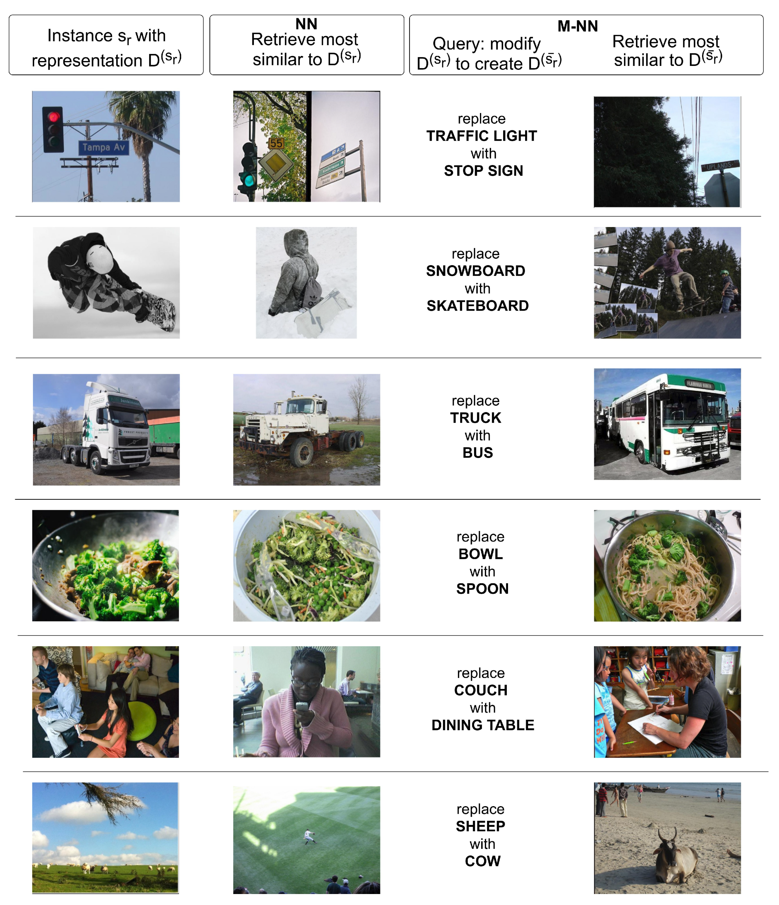
4.3. Retrieval
The experiments here are designed to show the interpretability, composability, and compressibility of the CoDiR representations. All models and baselines in these sections are pre-trained on the classification task above. We performed two types of retrieval experiments:
- (1)
- NN: the most similar instance to a reference instance is retrieved.
- (2)
- M-NN: an instance is retrieved with modified class membership while contextual information in the environments is retained. Specifically: “Given an input that belongs to class but not , retrieve the instance in the dataset that is most similar to that belongs to and not ”, where and are class labels (see Figure 2). We will show that CoDiR is well suited for such a task, as its structure can be exploited to create modified representations through decomposition as explained in Section 3.5.
This task is evaluated as shown in Table 3. Note that for the M-NN task, we want to evaluate two things: (1) to measure whether both labels were modified correctly, we evaluate the Precision (PREC) as a simple retrieval experiment where a retrieved example with the correctly modified classes is a true positive and a retrieved example with any incorrectly modified class is a false positive. (2) To indicate how well the contextual information is preserved after the modifications, the F1% score measures the proportion of the F1 score for the contextual caption words on the M-NN task over the F1 score for the contextual caption words on the NN task. The goal is then to achieve a good combination of M-NN PREC and F1% (for the latter, higher percentages are better). To clearly indicate that the F1% measures a proportion over F1 scores, we explicitly use a percentage notation for this score. For the sake of completeness, we also report the F1 score, precision, and recall over all classes in Appendix A.
We use the highly structured sigmoid outputs of the BXENT (single) and BXENT (joint) models as baselines, denoted as SEM (single) and SEM (joint), respectively. With SEM (joint), it is possible to directly modify class labels while maintaining all other information. It is thus a “best-case scenario”-baseline for which one can strive, as it combines a good M-NN precision and F1% score. SEM (single) on the other hand only contains class information and thus presents a best-case scenario for the M-NN precision score, yet a worst-case scenario for the F1% score. Additionally, we compare with a simple baseline consisting of Convolutional Neural Network (CNN) features from the penultimate layer of the BXENT (joint) models with . We also use those features in a Correlation Matching (CM) baseline, which combines different modalities (CNN features and word caption labels) into the same representation space [37]. The representations of these baseline models cannot be composed directly. In order to compare them to the “M-NN” method, therefore, we define templates as the average feature vector for a particular class. We then modify the representation for a instance s by subtracting the template of and adding the template of . All representations except SEM (single) are built from the BXENT (joint) models with . For CoDiR, they are built from CoDiR (capt) with .
For all baselines, similarity is computed with the cosine similarity, whereas for CoDiR, we exploit its structure as: over all classes c for which . Here, the notations are taken from Section 3.5, and is the modified representation of the reference instance. is the mean cosine similarity between and with the mean calculated over class dimensions. The similarity is thus calculated over class dimensions where classes with low relevance, i.e., those that have a low similarity with the templates, are not taken into account.
The advantages of the composability of the representations can be seen in Table 3 where CoDiR (capt) has a comparable performance to the fully semantic SEM (joint) representations. CNN (joint) manages to obtain a decent M-NN precision score, thus changing class information well, but at the cost of losing contextual information (low F1%), performing almost as poorly as SEM (single). Whereas CM performs well on the NN task, it does not change the class information accurately and thus (inadvertently) retains most contextual information. All baseline models require a cosine similarity, thus resulting in a time complexity of O(). For CoDiR, we see above that cosine similarities are computed over the environment dimension such that the time complexity becomes O().
We show some examples of retrieval results in Figure 2. In the first column, six example images from the test set are shown. For each example, the most similar image is retrieved and shown in the NN column. In the third column, a query is shown for the M-NN task that illustrates how the representation should be modified in order to create . In the last column, the most similar image is shown to the modified representation. The first three examples show successful results for both the NN and M-NN method. The fourth example shows a debatable result for M-NN where a spoon is now visible next to the dish, but it is not clear whether the food comes in a bowl or a pot. In Example 5, the M-NN method does show a table, but clearly not a dining table. The last example shows a failure case for the NN method where a baseball pitch is returned instead of a field with sheep. The M-NN method does return a cow, but on a beach rather than a grass field.
4.4. Rank
While the previous section shows that the structure of CoDiR representations provides access to semantic information derived from the labels on which they were trained, we hypothesize that the representations contain additional information beyond those labels, reflecting local, continuous features in the images. To investigate this hypothesis, we perform an experiment, similar to [38], to determine the rank of a matrix composed of 1000 instance representations of the test set. To maintain stability, we take only the first 3 rows (corresponding to 3 classes) and all 300 environments of each representation. Each of these is flattened into a 1D vector of size 900 to construct a matrix of size 1000 × 900. Small singular values are thresholded as set by [39]. The model used is the CoDiR (capt) ResNet-18 model with . We obtain a rank of 499, which exceeds the amount of class and environment labels (3+300) within, suggesting that the representations contain an additional structure beyond the original labels.
4.5. Compressed Representations
The representations can thus be compressed. Table 3 shows that C-CoDiR with , denoted as C-CoDiR(5), approaches CoDiR’s performance across all defined retrieval tasks. In Table 4, we show the performance on the retrieval task of Section 4.3 for compressed C-CoDiR(k) representations for different ranks k. It can be seen that the compressed representations still perform well up to . For extreme compressions where and , the performance on either the M-NN precision or the F1% metric deteriorates, which is to be expected as too much relevant information is lost.
4.6. Unseen Labels
To show that the CoDiR representations contain information beyond the pre-trained labels, we also use cross-validation to perform a binary classification task with a simple logistic regression. A subset of 400 images of dogs is taken from the validation and test sets, of which 24 and 17 respectively are positive examples of the previously unseen label: panting dogs. The logistic regression is performed with 2-fold cross-validation with an L2 penalty for regularization (the standard “LogisticRegression” implementation of the scikit-learn library was used for this computation, with the “lbfgs” solver and a maximum of 200 iterations for convergence). The inputs for the regression are the flattened representations of the input instances. The outcome in Table 5 shows that the CoDiR and C-CoDiR(5) representations outperform the purely semantic representations of the SEM model, which suggests that the additional continuous information is valuable. Nevertheless, the scores are overall quite low. Future work could expand on these results and further investigate the level of detail contained within the continuous-valued CoDiR embeddings.
4.7. Environment Composition
In this section, we investigate the properties of the environments, their composition, and their effect on the performance on the multi-label classification task of Section 4.2.
4.7.1. Hyperparameters
The performance of CoDiR depends on the parameters and R. To measure their influence, the multi-label classification task is performed for different values of these parameters.
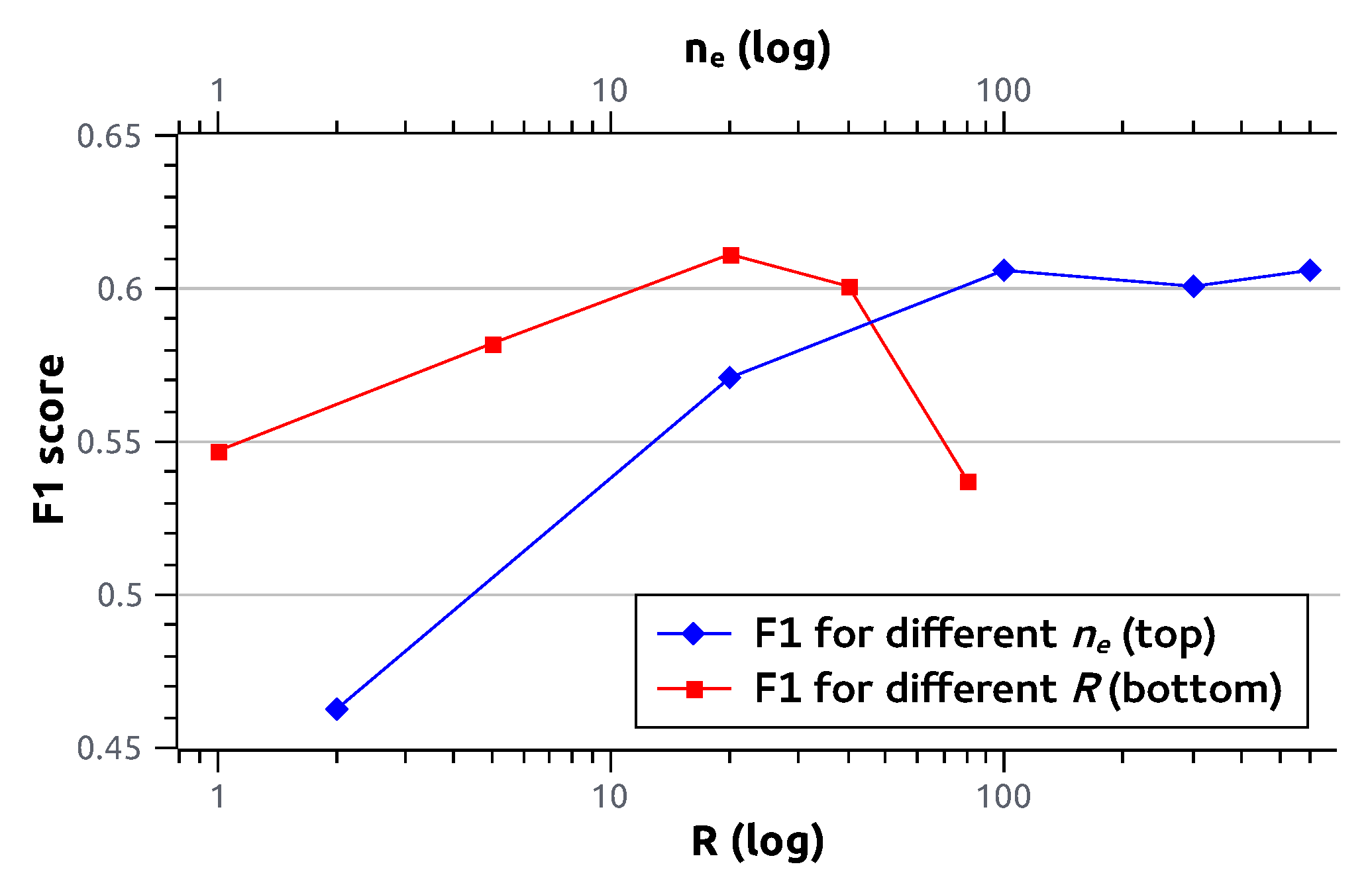
Increasing or the amount of environments (i.e., the amount of columns of the CoDiR representation) leads in general to better performance, although it plateaus after a certain level. Intuitively, this can be understood as follows: as more and more environments are chosen through a selection of random labels, the odds diminish that a new environment will add new, relevant, differentiating features. This is illustrated for the ResNet-18 CoDiR (class) approach to the multi-label classification problem of Section 4.2 in Figure 3.
For R, the maximum amount of labels per environment, an optimal value can be found empirically between 0 and . Combining a large amount of labels in any environment evidently creates a unique subset for comparison with instances. When R is too large, however, subsets with unique features are no longer created, and performance deteriorates. In Figure 3, the influence of R on the F1 score for multi-label image classification is also shown.
4.7.2. Sensitivity
A concern might be that classification results with our method would be highly sensitive to the choice of random environments. However, it turns out that even when and R are small, the outcome is not sensitive with regard to the choice of environments, suggesting that the amount and diversity are more important than the composition of the environments. This is shown in Table 6 and Table 7, which give the standard deviations of the F1 scores for different values of and R, respectively. This raises some interesting questions about the importance of the selected environments. We investigate these questions further in the following subsections.
4.7.3. Sufficient Number of Environments
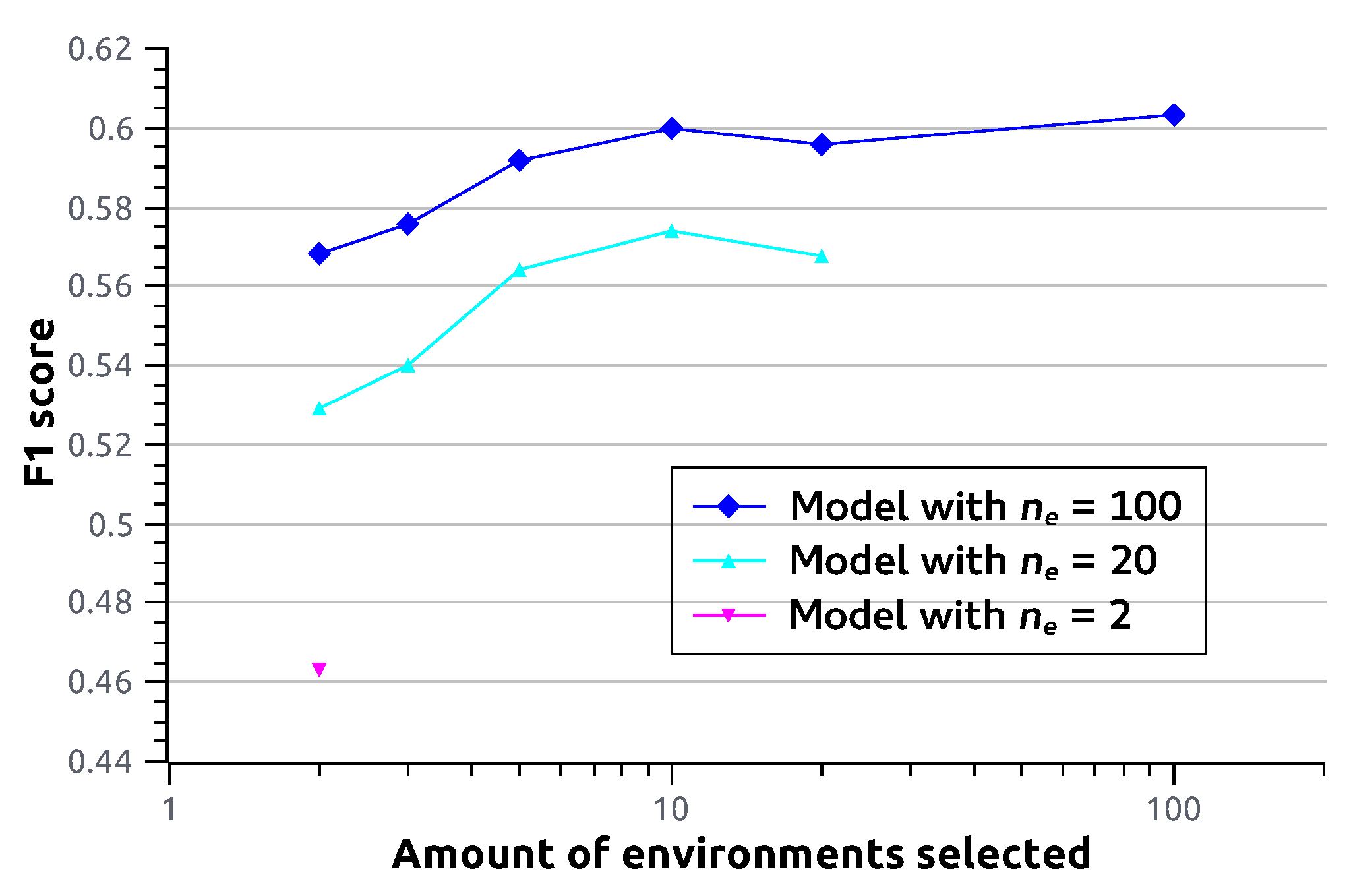
As the sensitivity of outcomes is relatively small even when a limited number of environments are used, it raises the question about how much the chosen environment compositions truly matter. Do models that are trained with more environments benefit because they have a better chance of containing more informative environments, or does a larger variety of environments help to learn better features at training time? To investigate this, we take the fully trained ResNet-18 CoDiR (class) models from Section 4.2 and only retain a number of environments where environments are selected randomly. We then perform the classification experiment from Section 4.2 again, but this time using the CoDiR representations with the reduced number of environments. Intuitively, we expect more selected environments to lead to better F1 scores. This is indeed the case, as can be seen in Figure 4, although the effect diminishes for larger . Interestingly, from this plot, it immediately becomes clear that two randomly selected environments from a model that was trained with a large number of environments (e.g., ) leads to better class membership estimations than from a model that was trained with a small number of environments (e.g., ). As the models are for the rest identical, there is nothing special about the selected environments. The reason why they thus outperform in this experiment must therefore be attributed to the larger number of environments during training, which thus leads to improved feature learning in the penultimate layer.
4.7.4. Number of Labels Per Environment
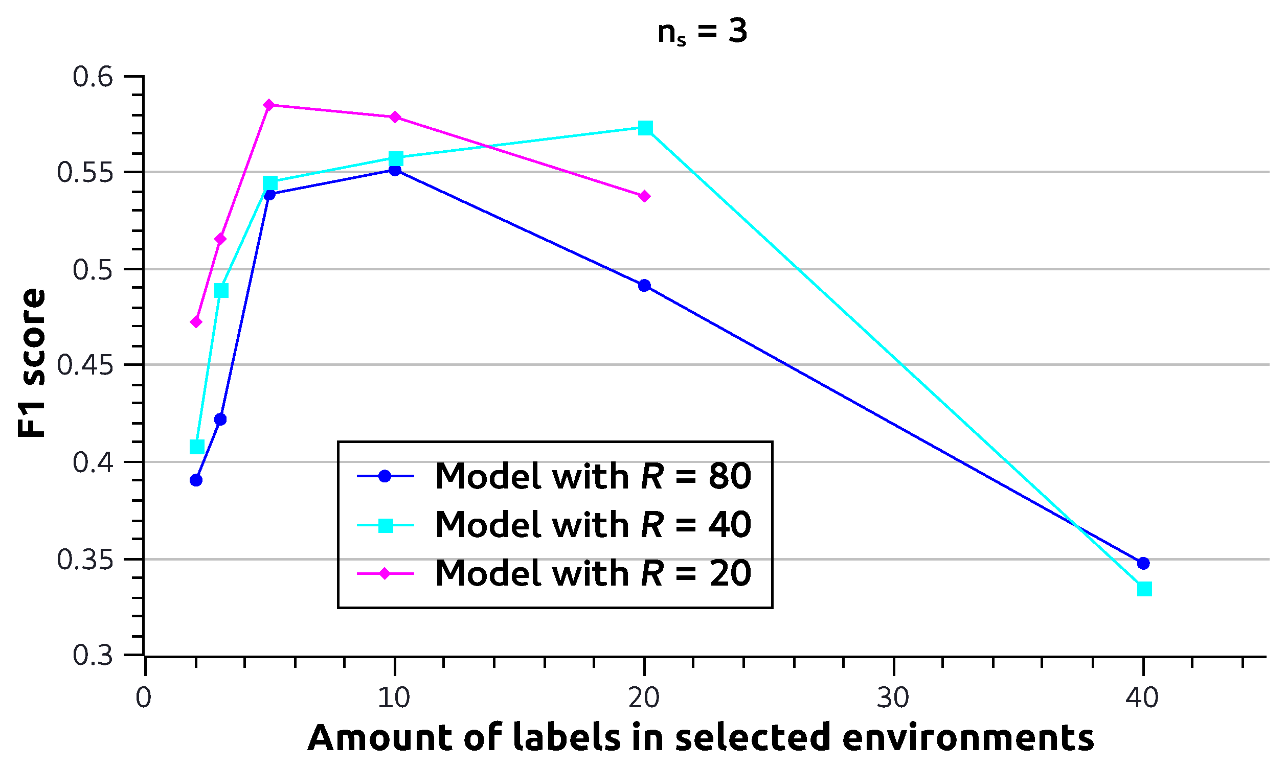
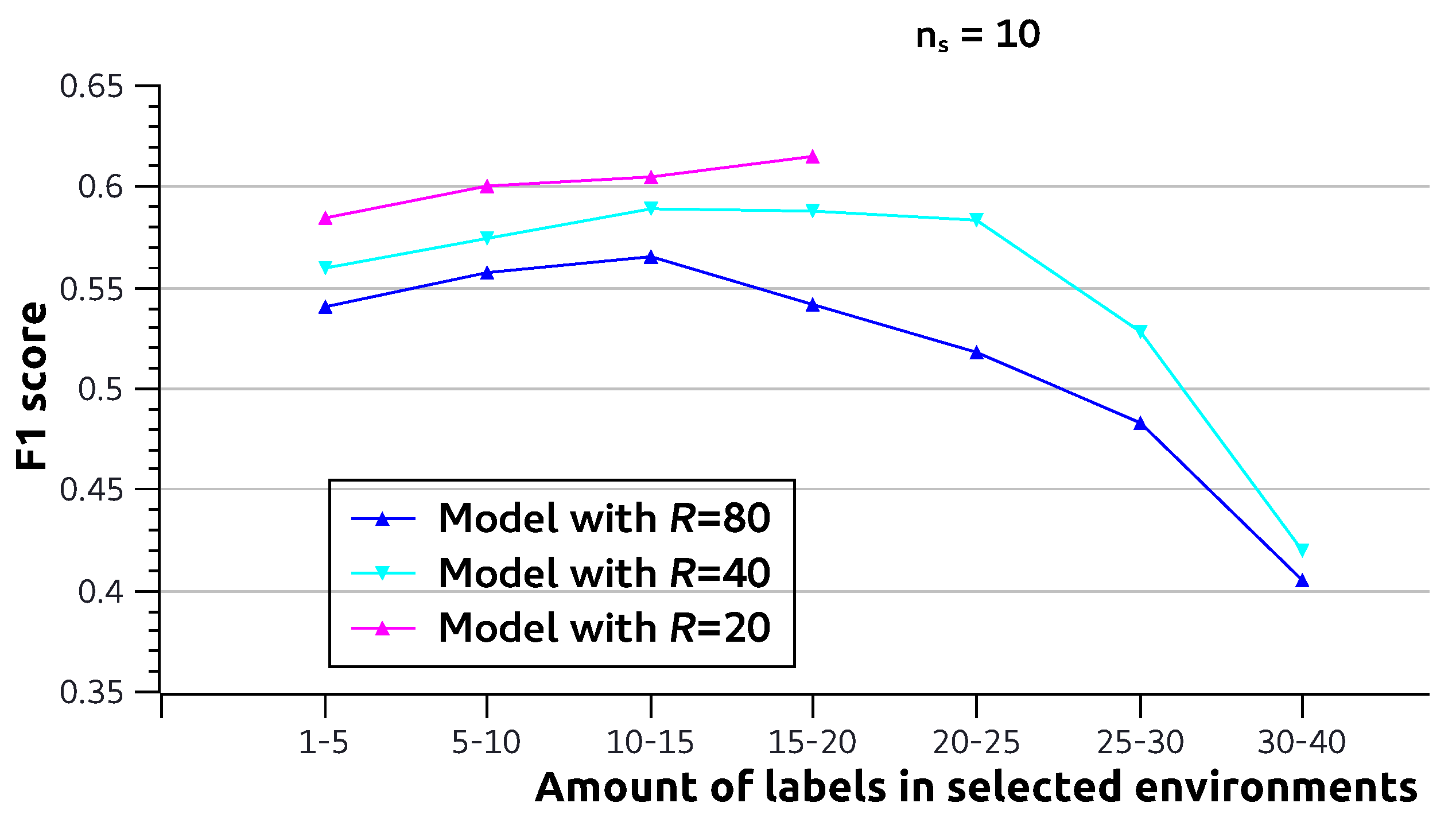
Another question is whether some environments contribute more to classification performance than others. To investigate this, we again take fully trained ResNet-18 CoDiR (class) models from Section 4.2. We again only retain a limited number of environments, denoted by , and perform the classification experiment from Section 4.2. However, instead of randomly selecting the environments, we selected environments that have a particular value of , i.e., the amount of labels in the environment. Figure 5 shows this for , where it becomes clear that environments with either small or large perform worse. Intuitively, this can be understood by the fact that an environment with will probably correspond to fewer images in the dataset. This might make it harder to estimate the distributional distance accurately. On the other hand, environments with large contain a very large amount of images in the dataset and most likely significantly overlap with many classes. This makes it harder to separate class from environment.
Finally, in Figure 6, we perform the same experiment, but now, we select environments. To allow enough environments for each value, we select the environments from ranges of . One can see here that the effect of small shown in Figure 5 is already largely diminished. However, the same is not true for large . This suggests that (1) some environments with small contain some complementary information and (2) environments with too large learn less useful features.
While the effect is thus relatively small, it could make sense to address the weight that is given to each environment. In this paper, a uniform distribution was assumed for in Equation (9), thus assigning equal weights. Two alternatives for future work can be formulated as a possible improvement to this approach: (1) assigning non-uniform weights to environments at inference time by modeling a more realistic ; or (2) ensuring that, while constructing environments, the randomly selected (class or caption) labels are sampled such that they are consistent with a uniform distribution for .
5. Discussion
CoDiR opens an interesting path for deep learning applications to explore the uses of structured representations, similar to how such structured matrices played a central role in many language processing approaches in the past. In zero-shot settings, the structure might be exploited, for example, to make compositions of classes and environments that were not seen before.
Whereas the current work focused on a multimodal setting for image and text, interesting applications can surely be found for other modality combinations. As an example, captions might help achieve increased action classification accuracy for videos. We also see a path to integrate useful information from more modalities into one representation by extending the 2D CoDiR structure into more dimensions. As CoDiR representations are obtained by calculating distances between distributions, it should be possible to do the same for marginal distributions from a multimodal distribution combining several modalities.
Additionally, further research might explore unsupervised learning. Both classes and environments might be handled in a symmetric manner by clustering relevant subsets of the dataset, for example. Similar to a k-means approach, initial cluster centers could be selected randomly or with a simple heuristic. Training set instances could then be assigned to the nearest cluster, and the cluster center could be updated iteratively over different batches. Downstream tasks could then potentially be performed on the learned representations from few examples.
Finally, as mentioned in Section 3.6, we use a Wasserstein-based distance to obtain relevant distance estimates for neural network-based instances. There is room to study other similarity or distance metrics in the context of such structure representations.
6. Conclusions
We introduce CoDiR, a novel deep learning method that creates multimodal, structured representations. With convolutional networks, labeled information from different modalities is used to project images into instance representations that are 2D structures where rows correspond to classes and columns to environments. Template representations are derived from instances to generalize over classes and are interpretable as distance estimates between respective classes and environments. In a multi-label classification task, it is demonstrated that CoDiR compares favorably to traditional cross-entropy-based methods, especially when environments are created from labels from image captions. Additionally, it is shown that as richer contextual information is added, performance increases. While the representations are continuous, they have a clear structure. We show in a retrieval task that this structure allows one to decompose the representations, modify particular content, and recompose them while maintaining existing information. The representations have a high rank and are also able to classify images with a logistic regression model according to a label that was never seen during the original training phase. Finally, the representations can also be compressed significantly while maintaining a large amount of information.
Author Contributions
Conceptualization, G.S. and M.-F.M.; methodology, G.S.; software, G.S.; writing, original draft preparation, G.S.; writing, review and editing, G.S. and M.-F.M.; visualization, G.S.; supervision, M.-F.M.; project administration, M.-F.M.; funding acquisition, M.-F.M. All authors have read and agreed to the published version of the manuscript.
Funding
This work was partly supported by the FWO and SNSF, Grants G078618N and #176004, as well as an ERC Advanced Grant, #788506.
Acknowledgments
We thank NVidia for granting us two TITAN Xp GPUs.
Conflicts of Interest
The authors declare no conflict of interest. The funders had no role in the design of the study; in the collection, analyses, or interpretation of data; in the writing of the manuscript; nor in the decision to publish the results.
Appendix A. Additional Retrieval Results
In Table A1 and Table A2, we add additional numbers for the retrieval results of the NN and M-NN experiments respectively from Section 4.3. In both cases, we report the F1 score, Precision (PREC), and Recall (REC) over all class labels. Note that for the M-NN experiment, we reported a different precision in Table 3, which was calculated over only the modified labels, to indicate clearly the impact of the modifications in the representations. The same conclusions can be drawn from both tables however.

Table A1.
For the NN retrieval experiment, we report performance metrics F1 score, Precision (PREC), and Recall (REC) over the class labels. Methods are used in combination with three different base models: ResNet-18/ResNet-101/Inception-v3. All results are the average of three runs.
Table A1.
For the NN retrieval experiment, we report performance metrics F1 score, Precision (PREC), and Recall (REC) over the class labels. Methods are used in combination with three different base models: ResNet-18/ResNet-101/Inception-v3. All results are the average of three runs.
| Method | F1 | PREC | REC |
|---|---|---|---|
| SEM (single) | 0.64/0.66/0.70 | 0.64/0.67/0.70 | 0.65/0.66/0.70 |
| SEM (joint) | 0.71/0.70/0.73 | 0.72/0.70/0.73 | 0.70/0.71/0.73 |
| CNN (joint) | 0.71/0.70/0.70 | 0.71/0.70/0.70 | 0.71/0.70/0.70 |
| CM | 0.72/0.74/0.74 | 0.73/0.73/0.72 | 0.72/0.74/0.76 |
| CoDiR | 0.70/0.72/0.72 | 0.68/0.70/0.71 | 0.71/0.73/0.72 |
| C-CoDiR (5) | 0.70/0.72/0.72 | 0.69/0.71/0.71 | 0.71/0.73/0.72 |
Table A2.
For the M-NN retrieval experiment, we report performance metrics F1 score, Precision (PREC), and Recall (REC) over the class labels. Methods are used in combination with three different base models: ResNet-18/ResNet-101/Inception-v3. All results are the average of three runs.
Table A2.
For the M-NN retrieval experiment, we report performance metrics F1 score, Precision (PREC), and Recall (REC) over the class labels. Methods are used in combination with three different base models: ResNet-18/ResNet-101/Inception-v3. All results are the average of three runs.
| Method | F1 | PREC | REC |
|---|---|---|---|
| SEM (single) | 0.69/0.69/0.72 | 0.68/0.68/0.71 | 0.69/0.70/0.73 |
| SEM (joint) | 0.64/0.65/0.66 | 0.63/0.64/0.65 | 0.64/0.66/0.66 |
| CNN (joint) | 0.67/0.60/0.65 | 0.66/0.60/0.64 | 0.67/0.60/0.66 |
| CM | 0.61/0.62/0.65 | 0.62/0.61/0.63 | 0.61/0.62/0.66 |
| CoDiR | 0.64/0.65/0.63 | 0.61/0.62/0.61 | 0.67/0.67/0.65 |
| C-CoDiR (5) | 0.64/0.64/0.63 | 0.61/0.61/0.62 | 0.67/0.67/0.65 |
References
- Murdock, B.B. A theory for the storage and retrieval of item and associative information. Psychol. Rev. 1982, 89, 609. [Google Scholar] [CrossRef]
- Nairne, J.S. The myth of the encoding-retrieval match. Memory 2002, 10, 389–395. [Google Scholar] [CrossRef]
- Hawkins, J.; Lewis, M.; Klukas, M.; Purdy, S.; Ahmad, S. A framework for intelligence and cortical function based on grid cells in the neocortex. Front. Neural Circuits 2019, 12, 121. [Google Scholar] [CrossRef]
- Salton, G.; Buckley, C. Term-weighting approaches in automatic text retrieval. Inf. Process. Manag. 1988, 24, 513–523. [Google Scholar] [CrossRef] [Green Version]
- Robertson, S.; Walker, S. Some simple effective approximations to the 2-Poisson model for probabilistic weighted retrieval. In Proceedings of the 17th Annual International ACM SIGIR Conference on Research and Development in Information Retrieval, Dublin, Ireland, 3–6 July 1994; pp. 232–241. [Google Scholar]
- Mikolov, T.; Chen, K.; Corrado, G.; Dean, J. Efficient estimation of word representations in vector space. arXiv 2013, arXiv:1301.3781. [Google Scholar]
- Peters, M.; Neumann, M.; Iyyer, M.; Gardner, M.; Clark, C.; Lee, K.; Zettlemoyer, L. Deep Contextualized Word Representations. In Proceedings of the 2018 Conference of the North American Chapter of the Association for Computational Linguistics: Human Language Technologies, New Orleans, LA, USA, 1–6 June 2018; Volume 1, pp. 2227–2237. [Google Scholar]
- Devlin, J.; Chang, M.W.; Lee, K.; Toutanova, K. BERT: Pre-training of Deep Bidirectional Transformers for Language Understanding. In Proceedings of the 2019 Conference of the North American Chapter of the Association for Computational Linguistics: Human Language Technologies, Minneapolis, MN, USA, 2–7 June 2019; Volume 1, pp. 4171–4186. [Google Scholar]
- Deerwester, S.; Dumais, S.T.; Furnas, G.W.; Landauer, T.K.; Harshman, R. Indexing by latent semantic analysis. J. Am. Soc. Inf. Sci. 1990, 41, 391–407. [Google Scholar] [CrossRef]
- Singh, S.P.; Hug, A.; Dieuleveut, A.; Jaggi, M. Context Mover’s Distance & Barycenters: Optimal transport of contexts for building representations. In Proceedings of the ICLR Workshop on Deep Generative Models, New Orleans, LA, USA, 6–9 May 2019. [Google Scholar]
- Hitchcock, F.L. The distribution of a product from several sources to numerous localities. J. Math. Phys. 1941, 20, 224–230. [Google Scholar] [CrossRef]
- Rubner, Y.; Tomasi, C.; Guibas, L.J. The earth mover’s distance as a metric for image retrieval. Int. J. Comput. Vis. 2000, 40, 99–121. [Google Scholar] [CrossRef]
- Sinkhorn, R. A relationship between arbitrary positive matrices and doubly stochastic matrices. Ann. Math. Stat. 1964, 35, 876–879. [Google Scholar] [CrossRef]
- Altschuler, J.; Niles-Weed, J.; Rigollet, P. Near-linear time approximation algorithms for optimal transport via Sinkhorn iteration. In Proceedings of the Advances in Neural Information Processing Systems 30, Long Beach, CA, USA, 4–9 December 2017; pp. 1964–1974. [Google Scholar]
- Arjovsky, M.; Chintala, S.; Bottou, L. Wasserstein Generative Adversarial Networks. In Proceedings of the 34th International Conference on Machine Learning, Sydney, Australia, 6–11 August 2017; pp. 214–223. [Google Scholar]
- Gulrajani, I.; Ahmed, F.; Arjovsky, M.; Dumoulin, V.; Courville, A.C. Improved training of wasserstein gans. In Proceedings of the Advances in Neural Information Processing Systems 30, Long Beach, CA, USA, 4–9 December 2017; pp. 5769–5779. [Google Scholar]
- Miyato, T.; Kataoka, T.; Koyama, M.; Yoshida, Y. Spectral Normalization for Generative Adversarial Networks. In Proceedings of the International Conference on Learning Representations, Vancouver, BC, Canada, 30 April–3 May 2018. [Google Scholar]
- Goodfellow, I.; Pouget-Abadie, J.; Mirza, M.; Xu, B.; Warde-Farley, D.; Ozair, S.; Courville, A.; Bengio, Y. Generative adversarial nets. In Proceedings of the Advances in Neural Information Processing Systems 28, Montreal, QC, Canada, 8–13 December 2014; pp. 2672–2680. [Google Scholar]
- Kusner, M.; Sun, Y.; Kolkin, N.; Weinberger, K. From Word Embeddings to Document Distances. In Proceedings of the 32nd International Conference on Machine Learning, Lille, France, 6–11 July 2015; pp. 957–966. [Google Scholar]
- Flamary, R.; Cuturi, M.; Courty, N.; Rakotomamonjy, A. Wasserstein discriminant analysis. Mach. Learn. 2018, 107, 1923–1945. [Google Scholar] [CrossRef] [Green Version]
- Johnson, W.B.; Lindenstrauss, J. Extensions of Lipschitz mappings into a Hilbert space. Contemp. Math. 1984, 26, 1. [Google Scholar]
- Candès, E.J.; Romberg, J.; Tao, T. Robust uncertainty principles: Exact signal reconstruction from highly incomplete frequency information. IEEE Trans. Inf. Theory 2006, 52, 489–509. [Google Scholar] [CrossRef] [Green Version]
- Donoho, D.L. Compressed sensing. IEEE Trans. Inf. Theory 2006, 52, 1289–1306. [Google Scholar] [CrossRef]
- Rahimi, A.; Recht, B. Random features for large-scale kernel machines. In Proceedings of the Advances in Neural Information Processing Systems 21, Vancouver, BC, Canada, 8–13 December 2008; pp. 1177–1184. [Google Scholar]
- Wu, L.; Yen, I.E.; Xu, K.; Xu, F.; Balakrishnan, A.; Chen, P.Y.; Ravikumar, P.; Witbrock, M.J. Word Mover’s Embedding: From Word2Vec to Document Embedding. In Proceedings of the 2018 Conference on EMNLP, Brussels, Belgium, 31 October–4 November 2018; pp. 4524–4534. [Google Scholar]
- Olah, C.; Mordvintsev, A.; Schubert, L. Feature visualization. Distill 2017, 2, e7. [Google Scholar] [CrossRef]
- Spinks, G.; Moens, M.F. Evaluating textual representations through image generation. In Proceedings of the Workshop on Analyzing and Interpreting Neural Networks for NLP, EMNLP, Brussels, Belgium, 31 October–4 November 2018. [Google Scholar]
- Zagoruyko, S.; Komodakis, N. Paying more attention to attention: Improving the performance of convolutional neural networks via attention transfer. arXiv 2016, arXiv:1612.03928. [Google Scholar]
- Higgins, I.; Matthey, L.; Pal, A.; Burgess, C.; Glorot, X.; Botvinick, M.; Mohamed, S.; Lerchner, A. Beta-vae: Learning basic visual concepts with a constrained variational framework. In Proceedings of the International Conference on Learning Representations, Toulon, France, 24–26 April 2017. [Google Scholar]
- Pandey, A.; Fanuel, M.; Schreurs, J.; Suykens, J.A. Disentangled Representation Learning and Generation with Manifold Optimization. arXiv 2020, arXiv:2006.07046. [Google Scholar]
- Mroueh, Y.; Sercu, T. Fisher gan. In Proceedings of the Advances in Neural Information Processing Systems 30, Long Beach, CA, USA, 4–9 December 2017; pp. 2513–2523. [Google Scholar]
- Rahimi, A.; Recht, B. Uniform approximation of functions with random bases. In Proceedings of the 2008 46th Annual Allerton Conference on Communication, Control, and Computing, Urbana-Champaign, IL, USA, 23–26 September 2008; pp. 555–561. [Google Scholar]
- Lin, T.Y.; Maire, M.; Belongie, S.; Hays, J.; Perona, P.; Ramanan, D.; Dollár, P.; Zitnick, C.L. Microsoft coco: Common objects in context. In Proceedings of the 13th European Conference on Computer Vision, Zurich, Switzerland, 6–12 September 2014; pp. 740–755. [Google Scholar]
- He, K.; Zhang, X.; Ren, S.; Sun, J. Deep residual learning for image recognition. In Proceedings of the IEEE Conference on Computer Vision and Pattern Recognition, Las Vegas, NV, USA, 26 June–1 July 2016; pp. 770–778. [Google Scholar]
- Szegedy, C.; Vanhoucke, V.; Ioffe, S.; Shlens, J.; Wojna, Z. Rethinking the inception architecture for computer vision. In Proceedings of the IEEE Conference on Computer Vision and Pattern Recognition, Las Vegas, NV, USA, 26 June–1 July 2016; pp. 2818–2826. [Google Scholar]
- Sorower, M.S. A literature survey on algorithms for multi-label learning. Or. State Univ. Corvallis 2010, 18, 1–25. [Google Scholar]
- Rasiwasia, N.; Costa Pereira, J.; Coviello, E.; Doyle, G.; Lanckriet, G.R.; Levy, R.; Vasconcelos, N. A new approach to cross-modal multimedia retrieval. In Proceedings of the 18th ACM International Conference on Multimedia, Firenze, Italy, 25–29 October 2010; pp. 251–260. [Google Scholar]
- Yang, Z.; Dai, Z.; Salakhutdinov, R.; Cohen, W.W. Breaking the Softmax Bottleneck: A High-Rank RNN Language Model. In Proceedings of the 6th International Conference on Learning Representations, Vancouver, BC, Canada, 30 April–3 May 2018. [Google Scholar]
- Press, W.H.; Teukolsky, S.A.; Vetterling, W.T.; Flannery, B.P. Numerical Recipes 3rd Edition: The Art of Scientific Computing; Cambridge University Press: Cambridge, UK, 2007. [Google Scholar]
Figure 1.
The last layer of a convolutional neural network is replaced with fully connected layers that map to outputs that are used to create instance representations that are interpretable along contextual dimensions, which we call “environments”. By computing the cosine similarity, rows are compared to corresponding class representations, which we refer to as “templates”.

Figure 2.
Example of retrieval results for both NNand M-NN. For NN, based on the representation , the most similar instance is retrieved. For M-NN, is modified into before retrieving the most similar instance.Retrieval example
Figure 2.
Example of retrieval results for both NNand M-NN. For NN, based on the representation , the most similar instance is retrieved. For M-NN, is modified into before retrieving the most similar instance.Retrieval example

Figure 3.
Influence of R and on the F1 score for multi-label image classification using the CoDiR (class) approach with ResNet-18. When modifying R, is fixed to 300. When modifying , R is fixed to 40. All data points are the average of three runs.Hyperparameters
Figure 3.
Influence of R and on the F1 score for multi-label image classification using the CoDiR (class) approach with ResNet-18. When modifying R, is fixed to 300. When modifying , R is fixed to 40. All data points are the average of three runs.Hyperparameters

Figure 4.
F1 score (y-axis) for multi-label image classification using the CoDiR (class) approach with ResNet-18. For models trained with different amounts of environments (), we perform multi-label classification while using only a portion of the environments. The amount of environments that are used () is shown on the x-axis. The environments used are selected randomly. All models are CoDiR (class) with and .

Figure 5.
F1 score (y-axis) for multi-label image classification using the CoDiR (class) approach with ResNet-18. For models trained with different maximum amounts of labels per environment (R), we perform multi-label classification while using only three of the available environments (). The x-axis indicates the number of labels the environments have (e.g., given , denotes the classification experiment where 3 environments were used for which in each case, ). All models are CoDiR (class) with and .F1 for different amount of labels for selected environments

Figure 6.
F1 score (y-axis) for multi-label image classification using the CoDiR (class) approach with ResNet-18. For models trained with different maximum amounts of labels per environment (R), we perform inference while using only 10 of the available environments (). The x-axis indicates the number of labels the environments have (e.g., given , “15–20” denotes the classification experiment where 10 environments were used for which in each case, is a value between 15 and 20). All models are CoDiR (class) with and .

Table 1.
Overview of the most important notations used in this paper.
| ci | Class label i. |
| The number of distinct class labels. | |
| The j-th environment. | |
| The number of environments. | |
| Environment label k, used to construct the environments. | |
| The number of distinct environment labels . | |
| R | The maximum number of labels per environment. |
| Random variable denoting the number of labels used to construct environment . | |
| Random variable denoting the m-th sampled label in environment . | |
| Instance representation for an instance x. | |
| Template representation for class . | |
| Function that computes the cosine similarity between two vectors. | |
| The threshold to determine class membership for class . |
Table 2.
F1 scores, Precision (PREC), and Recall (REC) for different models for the multi-label classification task. is the standard deviation of the F1 score over three runs. All results are the average of three runs. An asterisk * is added to indicate a model for which outperformance is statistically significant at a 0.05 significance level with respect to its corresponding baseline in a one-tailed t-test with unequal variances. The highest F1 score for each comparison is indicated in bold.
| MODEL | METHOD | R | F1 | PREC | REC | |||
|---|---|---|---|---|---|---|---|---|
| ResNet-18 | BXENT (single) | - | - | - | 0.566 | 0.579 | 0.614 | |
| ResNet-18 | CoDiR (class) | 300 | 91 | 40 | 0.601 * | 0.650 | 0.613 | |
| ResNet-101 | BXENT (single) | - | - | - | 0.570 | 0.582 | 0.623 | |
| ResNet-101 | CoDiR (class) | 300 | 91 | 40 | 0.627 * | 0.664 | 0.648 | |
| Inception-v3 | BXENT (single) | - | - | - | 0.638 | 0.663 | 0.669 | |
| Inception-v3 | CoDiR (class) | 300 | 91 | 40 | 0.617 | 0.648 | 0.646 | |
| ResNet-18 | BXENT (joint) | - | 300 | - | 0.611 | 0.631 | 0.654 | |
| ResNet-18 | BXENT (joint) | - | 1000 | - | 0.614 | 0.637 | 0.653 | |
| ResNet-18 | CoDiR (capt) | 300 | 300 | 40 | 0.629 * | 0.680 | 0.641 | |
| ResNet-18 | CoDiR (capt) | 1000 | 1000 | 100 | 0.638 * | 0.686 | 0.651 | |
| ResNet-101 | BXENT (joint) | - | 300 | - | 0.598 | 0.619 | 0.640 | |
| ResNet-101 | BXENT (joint) | - | 1000 | - | 0.592 | 0.611 | 0.638 | |
| ResNet-101 | CoDiR (capt) | 300 | 300 | 40 | 0.645 | 0.696 | 0.655 | |
| ResNet-101 | CoDiR (capt) | 1000 | 1000 | 100 | 0.657 * | 0.702 | 0.666 | |
| Inception-v3 | BXENT (joint) | - | 300 | - | 0.644 | 0.671 | 0.675 | |
| Inception-v3 | BXENT (joint) | - | 1000 | - | 0.63 | 0.655 | 0.663 | |
| Inception-v3 | CoDiR (capt) | 300 | 300 | 40 | 0.660 | 0.699 | 0.675 | |
| Inception-v3 | CoDiR (capt) | 1000 | 1000 | 100 | 0.661 | 0.700 | 0.676 |
Table 3.
For the NN and M-NN retrieval, the F1 score of class labels and the Precision (PREC) of the modified labels are shown for the first retrieved instance. The F1% score measures the proportion of the F1 score for the contextual caption words on the M-NN task over the F1 score for the contextual caption words on the NN task. A higher F1% score is better. Methods are used in combination with three different base models: ResNet-18/ResNet-101/Inception-v3. All results are the average of three runs.
| Method | NN | M-NN | |
|---|---|---|---|
| F1 | PREC | F1% | |
| SEM (single) | 0.64 /0.66/0.70 | 0.53/0.55/0.55 | 93/87/89 |
| SEM (joint) | 0.71/0.70/0.73 | 0.29/0.28/0.31 | 97/100/96 |
| CNN (joint) | 0.71/0.70/0.70 | 0.37/0.26/0.33 | 92/90/92 |
| CM | 0.72/0.74/0.74 | 0.19/0.15/0.18 | 100/100/100 |
| CoDiR | 0.70/0.72/0.72 | 0.30/0.30/0.27 | 97/97/95 |
| C-CoDiR(5) | 0.70/0.72/0.72 | 0.30/0.29/0.26 | 97/94/93 |
Table 4.
For different values of rank k, we show the effect of compression on the outcomes of the retrieval task. For the NN and M-NN retrieval setups, the F1 score of class labels and the Precision (PREC) of the modified labels are shown respectively for the first retrieved item. The F1% score measures the proportion of the F1 score for the contextual caption words on the M-NN task over the F1 score for the contextual caption words on the NN task. A higher F1% score is better. Values are shown for a ResNet-18 CoDiR (capt, ) model.
| Method | NN | M-NN | |
|---|---|---|---|
| F1 | PREC | F1% | |
| C-CoDiR(45) | 0.70 | 0.27 | 100 |
| C-CoDiR(23) | 0.70 | 0.28 | 99 |
| C-CoDiR(9) | 0.70 | 0.29 | 99 |
| C-CoDiR(5) | 0.70 | 0.29 | 98 |
| C-CoDiR(3) | 0.70 | 0.29 | 95 |
| C-CoDiR(1) | 0.70 | 0.17 | 100 |
Table 5.
F1 score for a simple logistic regression on pre-trained representations to classify a previously unseen label (“panting dogs”). For the last three models, . Methods are used in combination with three different base models: ResNet-18/ResNet-101/Inception-v3. All results are the average of three runs. Note that for cases where both precision and recall are zero, the F1 score is undefined. For simplicity and legibility, we write that in such cases, the F1 score is 0 as well.
| Method | F1 |
|---|---|
| SEM (single) | 0.00/0.00/0.00 |
| CoDiR (class) | 0.10/0.06/0.07 |
| C-CoDiR(5) (class) | 0.06/0.08/0.09 |
| SEM (joint) | 0.00/0.10/0.00 |
| CoDiR (capt) | 0.08/0.15/0.20 |
| C-CoDiR(5) (capt) | 0.10/0.14/0.19 |
Table 6.
Standard deviations of the F1 scores of the classification experiment for different values of . Each value is computed on the basis of three runs.
Table 6.
Standard deviations of the F1 scores of the classification experiment for different values of . Each value is computed on the basis of three runs.
Table 7.
Standard deviations of the F1 scores of the classification experiment for different values of R. Each value is computed on the basis of three runs.
Table 7.
Standard deviations of the F1 scores of the classification experiment for different values of R. Each value is computed on the basis of three runs.
© 2020 by the authors. Licensee MDPI, Basel, Switzerland. This article is an open access article distributed under the terms and conditions of the Creative Commons Attribution (CC BY) license (http://creativecommons.org/licenses/by/4.0/).
Share and Cite
MDPI and ACS Style
Spinks, G.; Moens, M.-F. Structured (De)composable Representations Trained with Neural Networks. Computers 2020, 9, 79. https://0-doi-org.brum.beds.ac.uk/10.3390/computers9040079
AMA Style
Spinks G, Moens M-F. Structured (De)composable Representations Trained with Neural Networks. Computers. 2020; 9(4):79. https://0-doi-org.brum.beds.ac.uk/10.3390/computers9040079
Chicago/Turabian StyleSpinks, Graham, and Marie-Francine Moens. 2020. "Structured (De)composable Representations Trained with Neural Networks" Computers 9, no. 4: 79. https://0-doi-org.brum.beds.ac.uk/10.3390/computers9040079
Note that from the first issue of 2016, this journal uses article numbers instead of page numbers. See further details here.