Minimal Complexity Support Vector Machines for Pattern Classification †

Kobe University, Kobe 657-8501, Japan
†
This paper is an extended version of our paper published in Abe, S. Minimal Complexity Support Vector Machines. In Artificial Neural Networks in Pattern Recognition. ANNPR 2020. Lecture Notes in Computer Science, Vol 12294; Schilling, F.P., Stadelmann, T., Eds.; Springer: Cham, Switzerland, 2020; pp. 89–101.
Computers 2020, 9(4), 88; https://0-doi-org.brum.beds.ac.uk/10.3390/computers9040088
Submission received: 15 September 2020
/
Revised: 23 October 2020
/
Accepted: 30 October 2020
/
Published: 4 November 2020
(This article belongs to the Special Issue Artificial Neural Networks in Pattern Recognition)
Abstract
:Minimal complexity machines (MCMs) minimize the VC (Vapnik-Chervonenkis) dimension to obtain high generalization abilities. However, because the regularization term is not included in the objective function, the solution is not unique. In this paper, to solve this problem, we discuss fusing the MCM and the standard support vector machine (L1 SVM). This is realized by minimizing the maximum margin in the L1 SVM. We call the machine Minimum complexity L1 SVM (ML1 SVM). The associated dual problem has twice the number of dual variables and the ML1 SVM is trained by alternatingly optimizing the dual variables associated with the regularization term and with the VC dimension. We compare the ML1 SVM with other types of SVMs including the L1 SVM using several benchmark datasets and show that the ML1 SVM performs better than or comparable to the L1 SVM.
1. Introduction
In the support vector machine (SVM) [1,2], training data are mapped into the high dimensional feature space, and in that space, the separating hyperplane is determined so that the nearest training data of both classes are maximally separated. Here, the distance between a data sample and the separating hyperplane is called margin. Thus, the SVM is trained so that the minimum margin is maximized.
Motivated by the success of SVMs in real world applications, many SVM-like classifiers have been developed to improve the generalization ability. The ideas of extensions lie in incorporating the data distribution (or margin distribution) to the classifiers because the SVM only considers the data that are around the separating hyperplane. If the distribution of one class is different from that of the other class, the separating hyperplane with the same minimum margin for both classes may not be optimal.
To cope with this, one approach proposes kernels based on the Mahalanobis distance [3,4,5,6,7,8,9,10]. Another approach reformulates the SVM such that the margin is measured by the Mahalanobis distance [11,12,13,14,15].
Yet another approach controls the overall margins instead of the minimum margin [16,17,18,19,20,21,22]. In [16], only the average margin is maximized. While the architecture is very simple, the generalization ability is inferior to that of the SVM [17,19]. To improve the generalization ability, the equality constraints were added in [19], but this results in the least squares SVM (LS SVM).
In [17], a large margin distribution machine (LDM) was proposed, in which the average margin is maximized and the margin variance is minimized. The LDM is formulated based on the SVM with inequality constraints. While the generalization ability is better than that of the SVM, the problem is that the LDM has one more hyperparameter than the SVM does. To cope with this problem, in [20,21], the unconstrained LDM (ULDM) was proposed, which has the equal number of hyperparameters and which has the generalization ability comparable to that of the LDM and the SVM.
The generalization ability of the SVM can be analyzed by the VC (Vapnik-Chervonenkis) dimension [1] and the generalization ability will be improved if the radius-margin ratio is minimized, where the radius is the radius of the minimum hypersphere that encloses all the training data in the feature space. The minimum hypersphere changes if the mapping function is changed during model selection, where all the parameter values including the value for the mapping function are determined, or feature selection is performed during training a classifier. So, minimization of the radius-margin ratio can be utilized in selecting the optimal mapping function [23,24]. In [25,26], feature selection is carried out during training by minimizing the radius-margin ratio.
If the center of the hypersphere is assumed to be at the origin, the hypersphere can be minimized for a given feature space as discussed in [27,28]. The minimal complexity machine (MCM) was derived based on this assumption. In the MCM, the VC dimension is minimized by minimizing the upper bound of the soft-margin constraints for the decision function. Because the regularization term is not included, the MCM is trained by linear programming. The quadratic version of the MCM (QMCM) tries to minimizes the VC dimension directly [28]. The generalization performance of the MCM is shown to be superior to that of the SVM, but according to our analysis [29], the solution is non-unique and the generalization ability is not better than that of the SVM. The problem of non-uniqueness of the solution is solved by adding the regularization term in the objective function of the MCM, which is a fusion of the MCM and the linear programming SVM (LP SVM) called MLP SVM.
In [30], to improve the generalization ability of the standard SVM (L1 SVM), we proposed fusing the MCM and the L1 SVM, which is the minimal complexity L1 SVM (ML1 SVM). We also proposed ML1 SVM, whose component is more similar to the L1 SVM. By the computer experiment using RBF (radius basis function) kernels, the proposed classifiers generalize better than or comparable to the L1 SVM.
In this paper we discuss the ML1 SVM and ML1 SVM more in detail, propose their training methods, prove their convergence, and demonstrate the effectiveness of the proposed classifiers using polynomial kernels in addition to RBF kernels.
The ML1 SVM is obtained by adding the upper bound on the decision function and the upper bound minimization term in the objective function of the L1 SVM. We show that this corresponds to minimizing the maximum margin. We derive the dual form of the ML1 SVM with one set of variables associated with the soft-margin constraints and the other set, upper-bound constraints. We then decompose the dual ML1 SVM into two subproblems: one for the soft-margin constraints, which is similar to the dual L1 SVM, and the other for the upper-bound constraints. These subproblems include neither the bias term nor the upper bound. Thus, for a convergence check, we derive the exact KKT (Karush-Kuhn-Tucker) conditions that do not include the bias term and the upper bound. The second subproblem is different from the first subproblem in that it includes the inequality constraint on the sum of dual variables. To remove this, we change the inequality constraint into two equality constraints and obtain ML1 SVM.
We consider training the ML1 SVM and ML1 SVM optimizing the first and the second subprograms, alternatingly. Because the ML1 SVM and ML1 SVM are very similar to the L1 SVM, we discuss the training method based on Sequential Minimum Optimization (SMO) fused with Newton’s method [31]. We also show the convergence proof of the proposed training methods. By computer experiments using polynomial kernels, in addition to RBF kernels, we compare the ML1 SVM and ML1 SVM with other classifiers including the L1 SVM.
In Section 2, we summarize the architectures of L1 SVM and the MCM. In Section 3, we discuss the architecture of the ML1 SVM and derive the dual form and the optimality conditions of the solution. Then, we discuss the architecture of the ML1 SVM. In Section 4, we discuss the training method that is an extension of SMO fused with Newton’s method [31] and the working set selection method. We also show the convergence proof of the proposed method. In Section 5, we evaluate the generalization ability of the ML1 SVM and other SVM-like classifiers using two-class and multiclass problems.
2. L1 Support Vector Machines and Minimal Complexity Machines
In this section, we briefly explain the architectures of the L1 SVM and the MCM [27]. Then we discuss the problem of non-unique solutions of the MCM and one approach to solving the problem [29].
2.1. L1 Support Vector Machines
Let M training data and their labels be , where is an n-dimensional input vector and for Class 1 and for Class 2. The input space is mapped into the l-dimensional feature space by the mapping function and in the feature space the separating hyperplane is constructed. The decision boundary given by the decision function is given by
where is the l-dimensional coefficient vector and b is the bias term.
The primal form of the L1 SVM is given by
where , is the slack variable for , and C is the margin parameter that determines the trade-off between the maximization of the margin and minimization of the classification error. Inequalities (3) are called soft-margin constraints.
The dual problem of (2) and (3) is given by
where , is the kernel function, , is the Lagrange multiplier for the ith inequality constraint, and associated with positive is called a support vector.
The decision function given by (1) is rewritten as follows:
where S is the set of support vector indices.
2.2. Minimal Complexity Machines
The VC (Vapnik-Chervonenkis) dimension is a measure for estimating the generalization ability of a classifier and lowering the VC dimension leads to realizing a higher generalization ability. For an SVM-like classifier with the minimum margin , the VC dimension D is bounded by [1]
where R is the radius of the smallest hypersphere that encloses all the training data.
In training the L1 SVM, both R and l are not changed. In the LS SVM, where are replaced with in (2) and the inequality constraints, with equality constraints in (3), although both R and l are not changed by training, the second term in the objective function works to minimize the square sums of . Therefore, like the LDM and ULDM, this term works to condense the margin distribution in the direction orthogonal to the separating hyperplane.
In [27], first the linear MCM, in which the classification problem is linearly separable, is derived by minimizing the VC-dimension, i.e., in (7). In the input space, R and are calculated, respectively, by
where 1 is added to to make the separating hyperplane passes through the origin in the augmented space. Equation (8) shows that the minimum hypersphere is also assumed to pass through the origin in the augmented space. After some derivations, the linear MCM is derived. The nonlinear MCM is derived as follows:
where h is the upper bound of the soft-margin constraints and . Here, the mapping function in (1) is [32]
and . The MCM can be solved by linear programming.
Because the upper bound h in (11) is minimized in (10), the separating hyperplane is determined so that the maximum distance between the training data and the separating hyperplane is minimized. This is a similar idea to that of the LS SVM, LDM, and ULDM.
The MCM is derived based on the minimization of the VC dimension, and thus considers maximizing the minimum margin. However, the MCM does not explicitly include the term related to the margin maximization. This makes the solution non-unique and unbounded.
To make the solution unique under the condition that the extended MCM still is a linear programming problem, in [29] we proposed the minimal complexity LP SVM (MLP SVM), which fuses the MCM an LP SVM:
where is the positive parameter and . Deleting in (13) and upper bound h in (14), we obtain the LP SVM. Setting and in (13), we obtain the MCM. Compared to the MCM and the LP SVM, the number of hyperparameters increases by 1.
According to the computer experiment, in general, the MLP SVM is better than the MCM and LP SVM in generalization abilities. However, it is inferior to the L1 SVM [29].
3. Minimal Complexity L1 Support Vector Machines
In this section, we discuss the ML1 SVM, which consists of two optimization subprograms and derive the KKT conditions that the optimal solution of the ML1 SVM must satisfy. Then, we discuss a variant of the ML1 SVM, whose two subprograms are more similar.
3.1. Architecture
The LDM and ULDM maximize the average margin and minimize the average margin variance and LS SVM makes data condense around the minimum margin. The idea of the MCM to minimize the VC dimension results in minimizing the maximum distance of the data from the separating hyperplane. Therefore, these classifiers have the idea in common: condense data as near as possible to the separating hyperplane.
In [29], we proposed fusing the MCM and the LP SVM. Similar to this idea, here we fuse the MCM given by (10) and (11) and the L1 SVM given by (2) and (3):
where , is the parameter to control the volume that the training data occupy, and h is the upper bound of the constraints. The upper bound defined by (11) is redefined by (17) and (18), which exclude . This makes the KKT conditions for the upper bound simpler. We call (17) the upper bound constraints and the above classifier minimum complexity L1 SVM (ML1 SVM). The right-hand side of (17) shows the margin with the minimum margin normalized to 1 if the solution is obtained. Therefore, because h is the upper bound of the margins and h is minimized in (15), the ML1 SVM maximizes the minimum margin and minimizes the maximum margin simultaneously.
If we use (12), we can directly solve (15) to (18). However, sparsity of the solution will be lost. Therefore, in a way similar to solving the L1 SVM, we solve the dual problem of (15) to (18).
Introducing the nonnegative Lagrange multipliers , , and , we obtain
where and .
For the optimal solution, the following KKT conditions are satisfied:
where is the zero vector whose elements are zero. Equations (24) to (27) are called KKT complementarity conditions.
Substituting (19) into (20) to (23) gives, respectively,
Substituting (28) to (31) into (19), we obtain the following dual problem:
The dual L1 SVM given by (4) and (5) is obtained by deleting variables and from the above optimization problem.
For the solution of (32) to (35), associated with positive or is a support vector. However, from (28), the decision function is determined by the support vectors that satisfy .
We consider decomposing the above optimization problem into two subproblems: (1) optimizing while fixing and (2) optimizing while fixing . To make this possible, we eliminate the interference between and in (33) by
Then the optimization problem given by (32) to (35) is decomposed into the following two subproblems:
Subproblem 1: Optimization of
where .
Subproblem 2: Optimization of
where Here we must notice that . If , from (41), at least
is satisfied. This contradicts (42).
We solve Subproblems 1 and 2 alternatingly until the solution converges. Subproblem 1 is very similar to the L1 SVM and can be solved by the SMO (Sequential minimal optimization). Subproblem 2, which includes the constraint (42) can also be solved by a slight modification of the SMO.
3.2. KKT Conditions
To check the convergence of Subproblems 1 and 2, we use the KKT complementarity conditions (24) to (27). However, variables h and b, which are included in the KKT conditions, are excluded from the dual problem given by (32) to (35). Therefore, as with the L1 SVM [33], to make an accurate convergence test, the exact KKT conditions that do not include h and b need to be derived.
We rewrite (24) as follows:
where
We can classify the conditions of (45) into the following three cases:
- .Because and ,
- Because , is satisfied. Therefore,
- .Because , is satisfied. Therefore,
Then the KKT conditions for (45) are simplified as follows:
where
To detect the violating variables, we define and as follows:
If the KKT conditions are satisfied,
The bias term is estimated to be
where is the estimate of the bias term using (24).
Likewise, using (46), (25) becomes
Then the conditions for (25) are rewritten as follows:
- .Fromwe have
- .
The KKT conditions for (25) are simplified as follows:
where , , and
To detect the violating variables, we define , , , and as follows:
In general, the distributions of Classes 1 and 2 data are different. Therefore, the upper bounds of h for Classes 1 and 2 are different. This may mean that either of () and may not exist. However, because of (41), both classes have at least one positive each, and because of (53), the values of h for both classes can be different. This happens because we separate (33) into two equations as in (36). Then, if the KKT conditions are satisfied, both of the following inequalities hold
From the first inequality, the estimate of h, for Class 2, is given by
From the second inequality, the estimate of h, for Class 1, is given by
3.3. Variant of Minimal Complexity Support Vector Machines
Subproblem 2 of the ML1 SVM is different from Subproblem 1 in that the former includes the inequality constraint given by (42). This makes the solution process more complicated. In this section, we consider making the solution process similar to that of Subproblem 1.
Solving Subproblem 2 results in obtaining and . We consider assigning separate variables and for Classes 1 and 2 instead of a single variable h. Then the complementarity conditions for and are
where and are the Lagrange multipliers associated with and , respectively. To simplify Subproblem 2, we assume that . This and (41) make (41) and (42) two equality constraints. Then the optimization problem given by (40) to (43) becomes
Here, (41) is not necessary because of (67). We call the above architecture ML1 SVM.
For the solution of the ML1 SVM, the same solution is obtained by the ML1 SVM with the value given by
However, the reverse is not true, namely, the solution of the ML1 SVM may not be obtained by the ML1 SVM. As the value becomes large, the value of becomes positive for the ML1 SVM, but for the ML1 SVM, the values of are forced to become larger.
4. Training Methods
In this section we extend the training method for the L1 SVM that fuses SMO and Newton’s method [31] for training the ML1 SVM. The major part of the training method consists of calculation of corrections by Newton’s method and the working set selection method. The training method of the ML1 SVM is similar to that of the L1 SVM. Therefore, we only explain the difference of the methods in Section 4.3.
4.1. Calculating Corrections by Newton’s Method
In this subsection, we discuss the corrections by Newton’s method for two subprograms.
4.1.1. Subprogram 1
First we discuss optimization of Subproblem 1. We optimize the variables in the working set , where W includes working set indices, fixing the remaining variables, by
Here .
We can solve the above optimization problem by the method discussed in [31]. We select in the working set and solve (71) for :
Substituting (73) into (70), we eliminate the equality constraint. Let . Now because is quadratic, we can express the change of , , as a function of the change of , , by
Then, neglecting the bounds, has the maximum at
where
Here, the partial derivative of Q with substitution of (73) is calculated by the chain rule without substitution.
We assume that is positive definite. If not, we avoid matrix singularity adding a small value to the diagonal elements.
Then from (73) and (75), we obtain the correction of :
For , if
we delete these variables from the working set and repeat the procedure for the reduced working set. Let be the maximum or minimum correction of that is within the bounds. Then if , . Moreover, if , . Otherwise Then we calculate
where r is the scaling factor.
The corrections of the variables in the working set are given by
4.1.2. Subprogram 2
We optimize the variables in the working set , fixing the remaining variables, by
We select in the working set W and solve (83) for :
Then similar to Subproblem 1, we substitute (86) into (82) and eliminate . The partial derivatives in (75) are as follows:
From (86), we obtain the correction of :
Now we consider the constraint (84). If , the sum of corrections needs to be zero. This is achieved if
Namely, we select the working set from the same class.
For , if
we delete these variables from the working set and repeat the procedure for the reduced working set. Let be the maximum or minimum correction of that is within the bounds. Then if , . Otherwise Then we calculate
where r is the scaling factor.
If , we further calculate
Then the corrections of the variables in the working set are given by
where r is replaced by if .
4.2. Working Set Selection
At each iteration of training, we optimize either Subproblem 1 () or Subproblem 2 (). To do so, we define the most violating indices as follows:
We consider that training is converged when
where is a small positive parameter.
If (96) is not satisfied, we correct variables associated with where i is determined by
According to the conditions of (96) and (97), we determine the variable pair as follows:
- If is the maximum in (97), we optimize Subproblem 1 (). Let the variable pair associated with and be and , respectively.
- If and either or is the maximum in (97), or if and either or exceeds but not both, we optimize Subproblem 2 ( belonging to either Class 1 or 2). Let the variable pair associated with and is either + or be and , respectively.
- If and both and exceed , we optimize Subproblem 2 ( selected from Classes 1 and 2). Let the variable pair be and . This is to make the selected variables correctable as will be shown in Section 4.4.2.
For the ML1 SVM, . Therefore, Case (3) is not necessary.
Because the working set selection strategies for and are the same, in the following we only discuss the strategy for .
In the first order SMO, at each iteration step, and that violate the KKT conditions the most are selected for optimization. This guarantees the convergence of the first order SMO [33]. In the second order SMO, the pair of variables that maximize the objective function are selected. However, to reduce computational burden, fixing , the variable that maximizes the objective function is searched [34]:
where is the set of indices that violate the KKT conditions:
We call the pair of variables that are determined either by the first or the second order SMO, SMO variables.
Because the second order SMO accelerates training for a large C value [35], in the following we use the second order SMO. However, for a substantially large C value, training speed of the second order SMO slows down because variables need to be updated many times to reach to the optimal values. To speed up convergence in such a situation, in addition to the SMO variables, we add variables that are selected in the previous steps as SMO variables, into the working set.
We consider that a loop is detected when at least one of the current SMO variables has already appeared as an SMO variable at a previous step. When a loop is detected, we pick up the loop variables that are the SMO variables in the loop. To avoid obtaining an infeasible solution by adding loop variables to the working set, we restrict loop variables to be unbounded support vectors, i.e., (This happens only for Subprogram 1).
Because we optimize Subprograms 1 and 2 alternatingly, loop variables may include those for Subprograms 1 and 2. Therefore, in optimizing Subprogram 1, we need to exclude the loop variables for Subproblem 2; and vice versa. In addition, in optimizing Subproblem 2 with , we need to exclude variables belonging to the unoptimized class, in addition to those for Subproblem 1.
If no loop is detected, the working set includes only the SMO variables. If a loop is detected, the working set consists of the SMO variables and the loop variables. For the detailed procedure, please refer to [31].
4.3. Training Procedure of ML1 SVM
In the following we show the training procedure of the ML1 SVM.
- (Initialization) Select and in the opposite classes and set , , , and , where .
- (Corrections) If Pr1 (Program 1), calculate partial derivatives (76) and (77) and calculate corrections by (75). Then, modify the variables by (81). Else, if Pr2, calculate partial derivatives (87) and (88) and calculate corrections by (75). Then, modify the variables by (94).
- (Convergence Check) Update and calculate , , , , , and . If (96) is satisfied, stop training. Otherwise if is the maximum, select Pr1, otherwise, Pr2. Calculate the SMO variables.
- (Loop detection and working set selection) Do loop detection and working set selection shown in the previous section and go to Step 2.
In Subproblem 2 of the ML1 SVM, data for Class 1 and Class 2 can be optimized separately. Therefore, because the data that are optimized belong to the same class, the sum of corrections is zero. Thus, in Step 1, . In Step 3, if Pr2 is optimized, the variables associated with or are optimized, not both.
4.4. Convergence Proof
Convergence of the first order SMO for the L1 SVM is proved in [33]. Similarly, we can prove that the training procedure discussed in Section 4.3 converges to the unique solution. In the following we prove the convergence for the ML1 SVM. The proof for the ML1 SVM is evident from the discussion.
Subprograms 1 and 2 are quadratic programming problems and thus have unique maximum solutions. Therefore, it is sufficient to prove that the objective function increases by the first order SMO. For the second order SMO, the increase of the objective function is also guaranteed because the variable pair that gives the largest increase of the objective function is selected. By combining SMO with Newton’s method, if some variables are not correctable, they are deleted from the working set. By this method, in the worst case, only the SMO variables remain in the working set. Therefore, we only need to show that the first order SMO converges for the ML1 SVM.
4.4.1. Convergence Proof for Subprogram 1
From (48), satisfies
Moreover, from (49), satisfies
Because the KKT conditions are not satisfied, . Moreover, we set . Then from (76) and (77),
where in (103), if the equality holds, we replace zero with a small negative value to avoid zero division in (75).
Then from (102), (103), and (75), the signs of the corrections and are given by
- and for ,
- and for ,
- and for ,
- and for .
From (100) and (101), the above corrections are all possible. For instance, in (1) and for . Therefore, .
Because the corrections are not zero, the objective function increases.
4.4.2. Convergence Proof for Subprogram 2
From (57) and (58), and satisfy
respectively. Likewise, from (59) and (60), and satisfy
respectively.
We set . Then from (87) and (88),
If we correct and , and . From (104), this correction is possible.
Likewise, if we correct and , and . From (105), this correction is possible.
If both and are larger than , we select and . Then from (104) and (105), these variables are correctable whether they be increased or decreased.
Because the corrections are not zero, the objective function increases.
5. Computer Experiments
First we analyze the behavior of the ML1 SVM and ML1 SVM using a two-dimensional iris dataset and then to examine the superiority of the proposed classifiers over the L1 SVM, we evaluate their generalization abilities and computation time using two-class and multiclass problems. All the programs used in the performance evaluation were coded in Fortran and tested using Windows machines.
5.1. Analysis of Behaviors
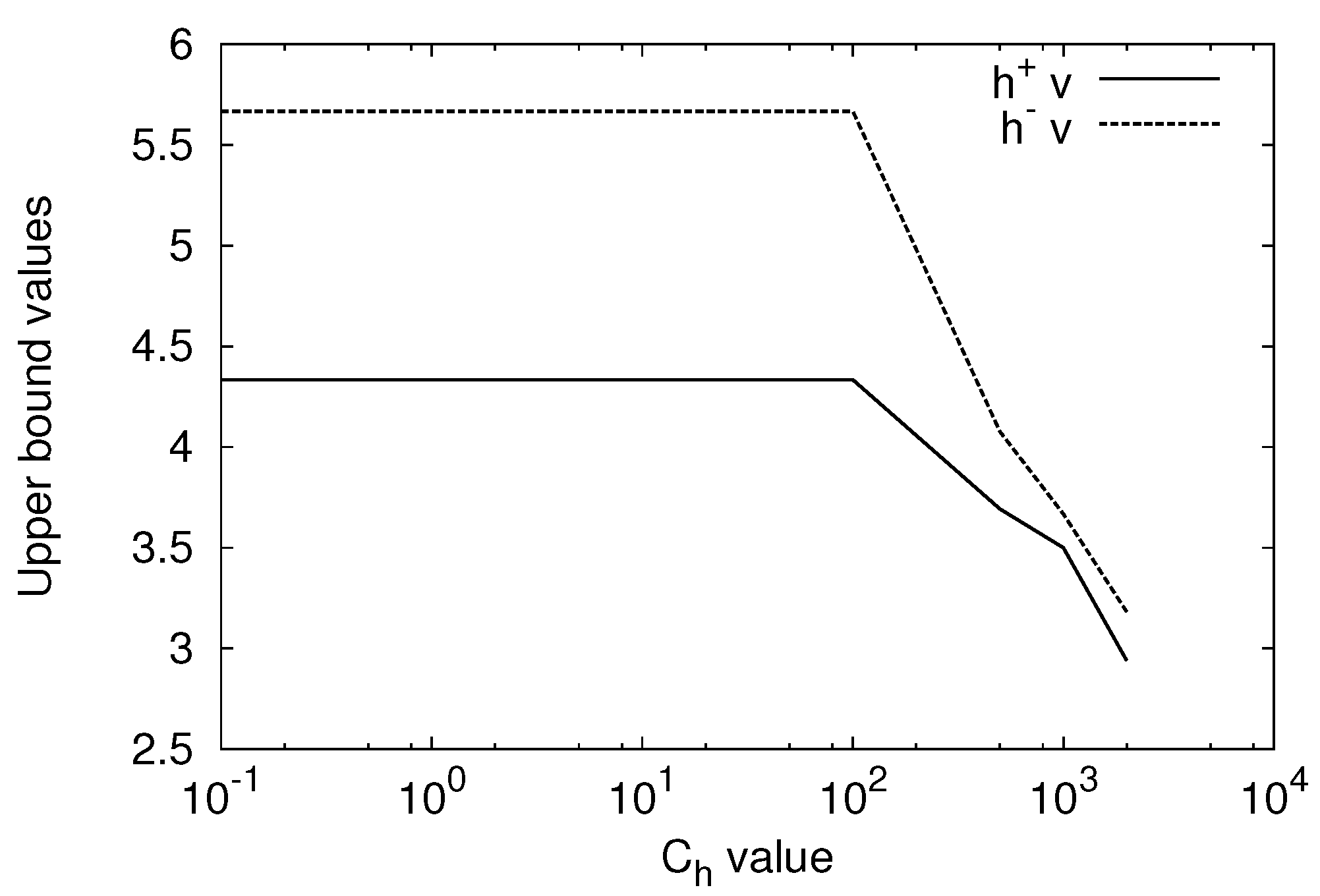
We analyzed the behaviors of the ML1 SVM and ML1 SVM using the iris dataset [36], which is frequently used in the literature. The iris dataset consists of 150 data with three classes and four features. We used Classes 2 and 3 and Features 3 and 4. For both classes, the first 25 data were used for training and the remaining data were used for testing. We used linear kernels: .
We evaluated the and values for the change of the value from 0.1 to 2000 fixing C to 1000. Figure 1 shows the result for the ML1 SVM. Both and values are constant for to 100 and they decrease as the value is increased. For the ML1 SVM, the and values are constant for the change of and are the same as those of the ML1 SVM with to 100. For , . Thus, For 10,000, . Thus, . This means that value is too small to obtain the solution comparable to that of the ML1 SVM. Therefore, the ML1 SVM is insensitive to the value compared to the ML1 SVM.
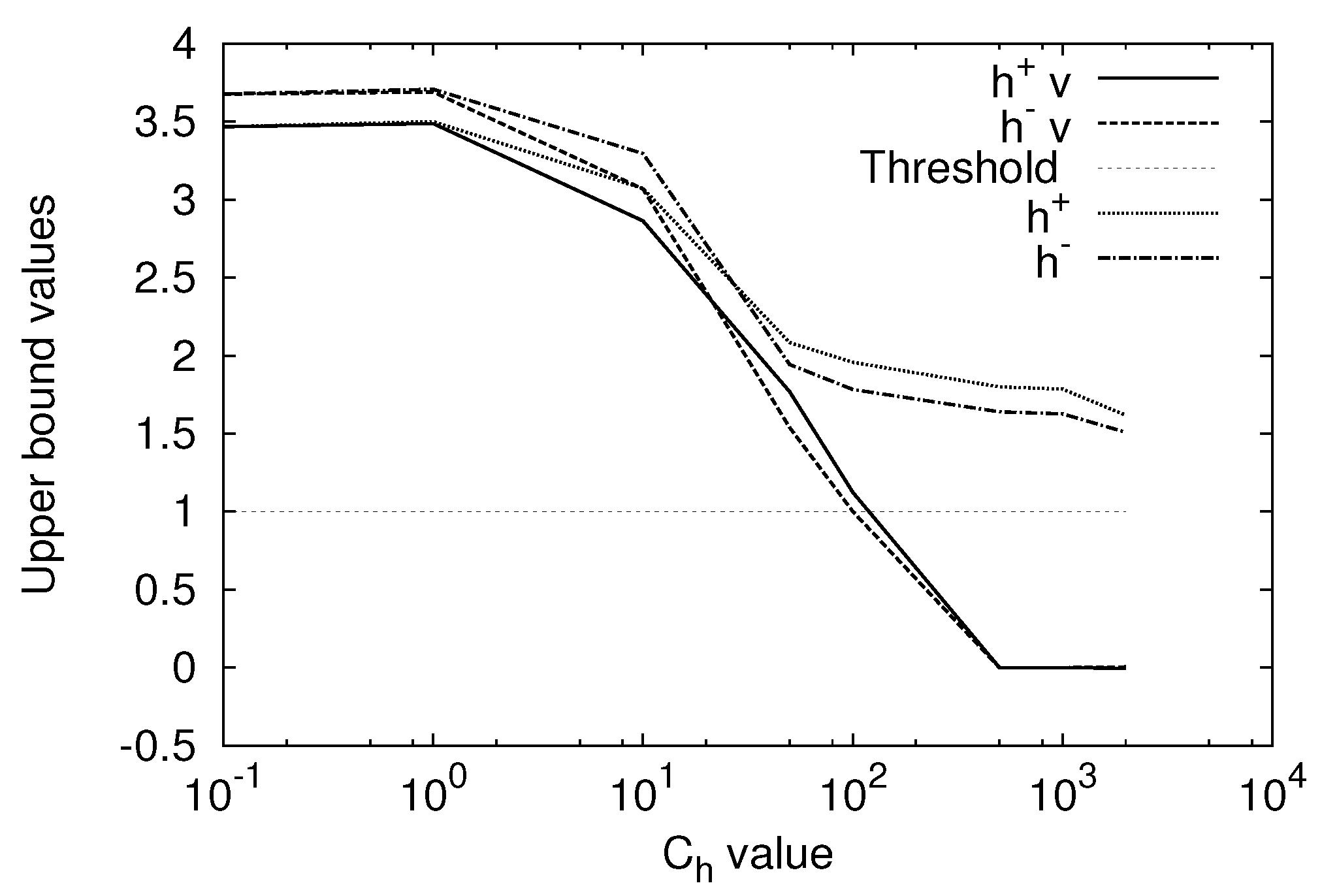
Figure 2 shows the and values for For the ML1 SVM, the and values become smaller than 1 for larger than 100. This means that the value is so large that the solution is no longer valid. However, for the ML1 SVM, the and values are larger than 1 and thus valid solutions are obtained for to 2000. This is because even at .
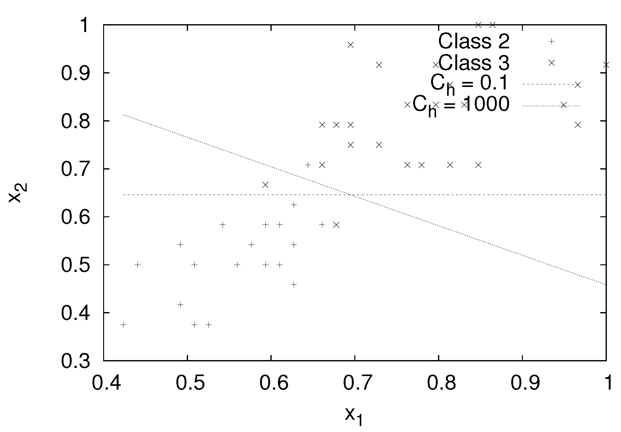
Figure 3 shows the decision boundary of the ML1 SVM for and , 1000. For , the decision boundary is almost parallel to the axis. However, for , the decision boundary rotates in the clockwise direction to make the data more condensed to the decision boundary. The accuracy for the test data is 92% for and is increased to 94% for .
From the above experiment we confirmed that the solutions of the ML1 SVM and the ML1 SVM are the same for small values but for large values both are different and in extreme cases the solution of the ML1 SVM may be infeasible.
5.2. Performance Comparison
In this section, we compare the generalization performance of the ML1 SVM and ML1 SVM with the L1 SVM, MLP SVM [29], LS SVM, and ULDM [20] using two-class and multiclass problems. Our main goal is to show that the generalization abilities of the ML1 SVM and ML1 SVM are better than the generalization ability of the L1 SVM.
5.2.1. Comparison Conditions
We determined the hyperparameter values using the training data by fivefold cross-validation, trained the classifier with the determined hyperparameter values, and evaluated the accuracy for the test data.
We trained the ML1 SVM, ML1 SVM, and L1 SVM by SMO combined with Newton’s method. We trained the MLP SVM by the simplex method and the LS SVM and ULDM by matrix inversion.
We used RBF kernels:
where is the parameter to control the spread of the radius and m is the number of inputs to normalize the kernel, and polynomial kernels including linear kernels:
where and for linear kernels and and for polynomial kernels.
In cross-validation, we selected the values for RBF kernels from , the d values for polynomial kernels from , and the C and values from . For the ULDM, the C value was selected from [21]. The value of in (99) was set to 0.01 for the ML1 SVM, ML1 SVM, and L1 SVM.
For the L1 SVM, LS SVM, and ULDM, we determined the and C values by grid search. For the ML1 SVM, ML1 SVM, and MLP SVM, we need to determined the value of in addition to and C values. (For the MLP SVM we evaluated the performance using only RBF kernels). To shorten computation time in such a situation, first we determined the and C values with for the MLP SVM) by grid search and then we determined the value by line search fixing the and C values with the determined values.
After model selection, we trained the classifier with the determined hyperparameter values and calculated the accuracy for the test data. For two-class problems, which have multiple sets of training and test pairs, we calculated the average accuracies and their standard deviations, and performed Welch’s t test with the confidence level of 5%.
5.2.2. Two-Class Problems
Table 1 lists the two-class problems used [37], which were generated using the datasets from the UC Irvine Machine Learning Repository [38]. In the table, the numbers of input variables, training data, test data, and training and test data pair sets are listed. The table also includes the maximum average prior probability shown in the accuracy (%). The numeral in parentheses shows that for the test data. According to the prior probabilities, the class data are relatively well balanced and there are not much differences between training and test data.
Table 2 shows the evaluation results using RBF kernels. In the table, for each classifier and each classification problem, the average accuracy and the standard deviation are shown. For each problem the best average accuracy is shown in bold and the worst, underlined. The “+” and “−” symbols at the accuracy show that the ML1 SVM is statistically better and worse than the classifier associated with the attached symbol, respectively. For instance, the ML1 SVM is statistically better than the ULDM for the flare-solar problem. The “Average” row shows the average accuracy of the 13 problems for each classifier and “B/S/W” denotes the number of times that the associated classifier show the best, the second best, and the worst accuracy. The “W/T/L” row denotes the number of times that the ML1 SVM is statistically better than, comparable to, and worse than the associated classifier.
According to the “W/T/L” row, the ML1 SVM is statistically better than the MLP SVM but is slightly inferior to ULDM. It is comparable to the remaining classifiers. From the “Average” measure, the ULDM is the best, the ML1 SVM, the second, the L1 SVM and the ML1 SVM, the third. From the “B/S/W” measure, the ULDM is the best and the LS SVM is the second best.
Table 3 shows the results for polynomial kernels. For each problem the best average accuracy is shown in bold and the worst, underlined. We do not include the MLP SVM for comparison. From the table, the ML1 SVM is statistically comparable to the L1 SVM, slightly better than ML1 SVM, and better than the LS SVM and ULDM. From the average accuracies, the L1 SVM is the best, ML1 SVM, the second best, and the ULDM, the worst.
The ML1 SVM is statistically inferior to ML1 SVM for the cancer and splice problems. We study why this happened. For the second file of the breast-cancer problem, the accuracy for the test data is 67.53% by the ML1 SVM, which is by 7.79% lower than by the ML1 SVM. The parameter values are selected as , , and . For the value higher than or equal to 50, the accuracy is 75.32%, which is the same as that by ML1 SVM. Therefore, model selection did not work properly. For the 17th file of the splice problem, the accuracy for the ML1 SVM is 83.68% with , and . This is caused by when the d and C values are determined by grid search. If , by model selection , are obtained, and the accuracy is 87.36%, which is better than 87.22% by the ML1 SVM. Therefore, in this case also, the low accuracy was obtained by the problem of model selection.
The ULDM performs worse than the ML1 SVM for banana and thyroid problems. For the banana problem by the ULDM, the average accuracy is by 6.66% lower than by the ML1 SVM. This was caused by mal-selection of the parameter ranges. By setting and , the average accuracy and standard deviation are 88.35 ± 1.10%, which are statistically comparable to those by the ML1 SVM. However, for the thyroid problem, the change of the parameter ranges does not improve the average accuracy much.
According to the experiment for the two-class problems, generally the accuracies using the RBF kernels are better than those using polynomial kernels, but for both RBF and polynomial kernels, the ML1 SVM, ML1 SVM, and L1 SVM perform well, while the LS SVM and ULDM do not for the polynomial kernels.
5.2.3. Multiclass Problems
We used pairwise (one-vs-one) classification for multiclass problems. To resolve unclassifiable regions occurred by pairwise classification, we used fuzzy classification, introducing the membership function for each decision function [2].
Table 4 shows the ten multiclass problems used for performance evaluation. Unlike the two-class problems, for each problem there is one training dataset and one test dataset. The numeral problem [2] is to classify numerals in the Japanese license plates, and the thyroid problem [38] is a medical diagnosis problem. The blood cell problem [2] classifies white blood cells labeled according to the maturity of the growing stage. Three hiragana problems [2] are to classify hiragana characters in the Japanese license plates. The satimage problem [38] classifies lands according to the satellite images. The USPS [39] and MNIST [40,41] problems treat numeral classification and the letter problem [38] treats alphabets. Because the original training dataset of the MNIST problem is too large especially for the LS SVM and ULDM, we switched roles of the training data and the test data.
Except for the thyroid problem, the class data are relatively well balanced. For the thyroid data, almost all data belong to one class. Moreover, the classification accuracy of a classifier smaller than 92.41% is meaningless.
Table 5 lists the accuracies using the RBF kernels for the test data. For each problem, the best accuracy is shown in bold, and the worst, underlined. For the MLP SVM, the accuracies for the thyroid, MNIST, and letter problems were not available. The “Average” row shows the average accuracy of the associated classifier for the ten problems and “B/S/W” shows the numbers of times that the best, the second best, and the worst accuracies are obtained. Among the ten problems, the accuracies of the ML1 SVM and ML1 SVM are better than or equal to those of the L1 SVM for nine and eight problems, respectively. In addition, the best average accuracy is obtained for the ML1 SVM, the second best, the ML1 SVM, and the third best, the L1 SVM. This is very different from the two-class problems where the ML1 SVM and ML1 SVM are comparable to the L1 SVM.
Table 6 shows the accuracies of the test data using polynomial kernels. For each problem the best accuracy is shown in bold and the worst, underlined. From the average accuracy, the ML1 SVM performs best, LS SVM performs the second best, and the L1 SVM and ULDM the worst. The difference between the LS SVM and ML1 SVM is very small. Improvement of the ML1 SVM and ML1 SVM over the L1 SVM is larger than that using the RBF kernels. For all the 10 problems, they are better than or equal to the L1 SVM. However, as seen from the Average rows in Table 5 and Table 6, the accuracies using polynomial kernels are in general worse than those using RBF kernels. The reason for this is not clear but the ranges of parameter values in model selection might not be well tuned for polynomial kernels.
In the previous experiment we evaluated RBF kernels and polynomial kernels separately, but we can choose the best kernel from RBF and polynomial kernels. If we have cross-validation results for both kernels, we can select the better one that has the higher accuracy. Table 7 shows the accuracies by cross-validation for RBF and polynomial kernels. For each problem and for each classifier, the better accuracy is shown in bold. The last row of the table shows the average accuracies. The average accuracies for the polynomial kernels are worse than those for the RBF kernels for all the classifiers. For each classifier, the number of problems that the polynomial kernels perform better or equal is one to two. Moreover, if we select RBF kernels when both average accuracies are the same, selecting kernels with the better average accuracy results in improving the accuracy for the test dataset as seen from Table 5 and Table 6. However, employing polynomial kernels in addition to RBF kernels does not improve the accuracy significantly.
5.3. Training Time Comparison
First, we examine the complexity of computation for each classifier excluding the MLP SVM. We trained the ML1 SVM, ML1 SVM, and L1 SVM by SMO combined with Newton’s method. Therefore, the complexity of computation for the subproblem with working set size W is . Because the ML1 SVM and ML1 SVM solve two quadratic programming programs, each having the same number of variables, M, the complexity of computation is the same with that of the L1 SVM. Therefore, the three classifiers are considered to be trained in comparable time.
Because the matrices associated with the LS SVM and ULDM are positive definite, they can be solved by iterative methods such as stochastic gradient methods [17]. However, we trained the LS SVM and ULDM by Cholesky factorization to avoid the inaccuracy caused by insufficient convergence. Therefore, the complexity of computation of both methods is .
The purpose of this section is to confirm that the ML1 SVM, ML1 SVM, and L1 SVM can be trained in comparable time.
Excluding that of the MLP SVM, we compared the time for training and testing a classifier using a Windows machine with 3.2 GHz CPU and 16 GB memory. For the two-class problems, we set the parameter values with the frequently selected values and trained the classifier using a training dataset and tested the trained classifier using the associated test dataset. For the multiclass problems, we trained a classifier with the parameter values obtained by cross-validation and tested the trained classifier with the test dataset.
Because the tendency is similar we only show the results using RBF kernels. Table 8 shows the parameter values selected for the two-class and multiclass problems. In the table Thyroid (m) denotes the multiclass thyroid problem. For each problem, the values in bold, the and C values in bold, and , C, and values in bold show that they appear more than once.
From the table, it is clear that the ML1 SVM, ML1 SVM, and L1 SVM selected the same and C values frequently and the ML1 SVM and ML1 SVM selected the same , C, and values 10 times out of 23 problems.
Table 9 sows the CPU time for training and test with the optimized parameter values listed in Table 8. For each problem the shortest CPU time is shown in bold and the longest, underlined. The CPU time for the two-class problem is that per file. For the multiclass problems, we used fuzzy pairwise classification. Therefore, the training time includes that for determining decision functions where n is the number of classes. For example, for the letter problem, 329 decision functions need to be determined. The last row of the table shows the numbers of times that the associated classifier are the fastest (B), the second fastest (S), and the slowest (W).
From the table, the ML1 SVM and ML1 SVM show comparable computation time. Moreover, except for the hiragana-50, hiragana-13, hiragana-105, USPS, MNIST, and letter problems, computation time for the ML1 SVM and ML1 SVM is comparable to that of the L1 SVM. For these problems, the ML1 SVM and ML1 SVM are much slower than L1 SVM. Analyzing the convergence process, we found that for these problems, monotonicity of the objective function value was sometimes violated. To improve convergence, we need to clarify why it happens and to find a way to speed up training in such a situation. However we leave this problem in the future study.
5.4. Discussions
As discussed in Section 3.3, the ML1 SVM and ML1 SVM are equivalent for a small value but for a large value they are different. The computer experiments in Section 5.1 also revealed that the ML1 SVM is insensitive to the change of a value. However, the difference of the generalization performance between the ML1 SVM and ML1 SVM is not large for the two-class and multiclass problems.
The execution time for the ML1 and ML1 SVM was sometimes longer than that for the L1 SVM. This will cause problem in model selection. While we leave the discussions of speeding up training, for the model selection, this problem may be alleviated for the ML1 SVM. If or is satisfied, the solution is infeasible. Therefore, we can skip cross-validation at the current value and the larger ones.
We used line search to speed up cross-validation. If grid search was used, in fivefold cross-validation we needed to train the ML1 SVM or ML1 SVM 3520 times, instead of 480 times. The speed up ratio is estimated to be 7.3. We evaluated the difference between the grid search and line search for the heart problem. We measured the execution time of cross-validation, training the classifier with the determined parameter values, and testing the classifier using the test data. For the ML1 SVM, the speed up ratio by line search was 35.7, and the average accuracy with the standard deviation of the grid search was 82.78 ± 3.45%, which was slightly lower. By the ML1 SVM, the speed up ratio was 40.0, and the average accuracy with the standard deviation was 82.85 ± 3.31%, which was also lower than that by line search. Therefore, because model selection slowed down very much and the improvement of the average accuracy was not obtained at least for the heart problem, grid search will not be a good selection.
To speed up model selection of the ML1 SVM or ML1 SVM, we may use the L1 SVM considering that the same values were selected frequently for the and C values (see Table 8 for values). For the multiclass problems, four problems do not have the same values. To check whether the idea works, we performed model selection of values fixing the values of and C determined by model selection of the L1 SVM for the hiragana-13, hiragana-105, USPS, and letter problems. Among the four problems, the ML1 SVM and ML1 SVM performed worse than the L1 SVM for the letter problem. Moreover, the resulting average accuracies of the ML1 SVM and ML1 SVM for ten problems were 97.14% and 97.16%, respectively, which were lower than by the original model selection by 0.03% (see Table 5) but were still better than the accuracy of the L1 SVM. If we switch back the roles of the training and test data for the MNIST problem, the selected parameter values for the L1 SVM were the same. The accuracies for the test data were 98.55%, 98.77%, and 98.78% for the L1 SVM, ML1 SVM, and ML1 SVM, respectively.
For the polynomial kernels, different kernel parameters were selected for six problems: the numeral (only for the ML1 SVM), blood cell, hiragana-50, hiragana-13, hiragana-105, and USPS problems. For each problem we determined the value by cross-validation fixing the values of d and C determined by the L1 SVM. The accuracies for the test datasets were all better than or equal to those by the L1 SVM. The average accuracies of the ML1 SVM or ML1 SVM for all the ten problems were 96.53% and 96.64%, respectively, which were lower than by the original model selection by 0.19% and 0.12%, respectively. For the MNIST problem with the switched training and test data, the selected parameter values for the L1 SVM were the same. Moreover, the accuracies for the test data were 98.17%, 98.23%, and 98.34% for the L1 SVM, ML1 SVM, and ML1 SVM, respectively.
6. Conclusions
The minimal complexity machine (MCM) minimizes the VC dimension and generalizes better than the standard support vector machine (L1 SVM). However, according to our previous analysis, the solution of the MCM is non-unique and unbounded.
In this paper, to solve the problem of the MCM and to improve the generalization ability of the L1 SVM, we fused the MCM and the L1 SVM, namely, we introduced minimizing the upper bound of the absolute decision function values to the L1 SVM. This corresponds to minimizing the maximum margin. Converting the original classifier into dual one, we derived two subproblems: the first subproblem corresponds to the L1 SVM and the second subproblem corresponds to minimizing the upper bound. We further modified the second subproblem by converting the inequality constraint into two equality constraints: one for optimizing the variables associated with the positive class and the other for the negative class. We call this architecture ML1 SVM and the original architecture, ML1 SVM.
We derived the exact KKT conditions for the first and second subproblems that exclude the bias term and the upper bound and discussed training the two subproblems alternatingly, fusing sequential minimal optimization (SMO) and Newton’s method.
According to computer experiments of the two-class problems using RBF kernels, the average accuracy of the ML1 SVM is statistically comparable to that of the ML1 SVM and L1 SVM. Using polynomial kernels, the ML1 SVM is statistically comparable to the L1 SVM but is slightly better than ML1 SVM.
For the multiclass problems using RBF kernels, the ML1 SVM and ML1 SVM generalize better than the L1 SVM and the ML1 SVM performs best, and the ML1 SVM, the second, among six classifiers tested. Using polynomial kernels, the ML1 SVM performs best, the LS SVM the second best, ML1 SVM the third, and the L1 SVM worst.
Therefore, the idea of minimizing the VC dimension for the L1 SVM worked to improve the generalization ability of the L1 SVM.
Execution time for the ML1 SVM and ML1 SVM is comparable to that for the L1 SVM for most of the problems tested, but in some problems, execution time is much longer. In the future study, we would like to clarify the reason and propose a fast training method in such cases. Another study will be to consider robustness for outliers by the soft upper bound, instead of the hard upper bound.
Funding
This work was supported by JSPS KAKENHI Grant Number 19K04441.
Conflicts of Interest
The author declares no conflict of interest. The founding sponsors had no role in the design of the study; in the collection, analyses, or interpretation of data; in the writing of the manuscript, and in the decision to publish the results.
References
- Vapnik, V.N. Statistical Learning Theory; John Wiley & Sons: New York, NY, USA, 1998. [Google Scholar]
- Abe, S. Support Vector Machines for Pattern Classification, 2nd ed.; Springer: London, UK, 2010. [Google Scholar]
- Abe, S. Training of Support Vector Machines with Mahalanobis Kernels. In Artificial Neural Networks: Formal Models and Their Applications (ICANN 2005)—Proceedings of Fifteenth International Conference, Part II, Warsaw, Poland; Duch, W., Kacprzyk, J., Oja, E., Zadrożny, S., Eds.; Springer-Verlag: Berlin, Germany, 2005; pp. 571–576. [Google Scholar]
- Wang, D.; Yeung, D.S.; Tsang, E.C.C. Weighted Mahalanobis Distance Kernels for Support Vector Machines. IEEE Trans. Neural Netw. 2007, 18, 1453–1462. [Google Scholar] [CrossRef]
- Shen, C.; Kim, J.; Wang, L. Scalable Large-Margin Mahalanobis Distance Metric Learning. IEEE Trans. Neural Netw. 2010, 21, 1524–1530. [Google Scholar] [CrossRef] [Green Version]
- Liang, X.; Ni, Z. Hyperellipsoidal Statistical Classifications in a Reproducing Kernel Hilbert Space. IEEE Trans. Neural Netw. 2011, 22, 968–975. [Google Scholar] [CrossRef]
- Fauvel, M.; Chanussot, J.; Benediktsson, J.; Villa, A. Parsimonious Mahalanobis kernel for the classification of high dimensional data. Pattern Recognit. 2013, 46, 845–854. [Google Scholar] [CrossRef] [Green Version]
- Reitmaier, T.; Sick, B. The responsibility weighted Mahalanobis kernel for semi-supervised training of support vector machines for classification. Inf. Sci. 2015, 323, 179–198. [Google Scholar] [CrossRef] [Green Version]
- Jiang, H.; Ching, W.K.; Yiu, K.F.C.; Qiu, Y. Stationary Mahalanobis kernel SVM for credit risk evaluation. Appl. Soft Comput. 2018, 71, 407–417. [Google Scholar] [CrossRef]
- Sun, G.; Rong, X.; Zhang, A.; Huang, H.; Rong, J.; Zhang, X. Multi-Scale Mahalanobis Kernel-Based Support Vector Machine for Classification of High-Resolution Remote Sensing Images. Cogn. Comput. 2019. [Google Scholar] [CrossRef]
- Lanckriet, G.R.G.; Cristianini, N.; Bartlett, P.; Ghaoui, L.E.; Jordan, M.I. Learning the Kernel Matrix with Semidefinite Programming. J. Mach. Learn. Res. 2004, 5, 27–72. [Google Scholar]
- Shivaswamy, P.K.; Jebara, T. Ellipsoidal Kernel Machines. In Proceedings of the Eleventh International Conference on Artificial Intelligence and Statistics (AISTATS 2007), San Juan, Puerto Rico, 21–24 March 2007. [Google Scholar]
- Xue, H.; Chen, S.; Yang, Q. Structural Regularized Support Vector Machine: A Framework for Structural Large Margin Classifier. IEEE Trans. Neural Netw. 2011, 22, 573–587. [Google Scholar] [CrossRef]
- Peng, X.; Xu, D. Twin Mahalanobis distance-based support vector machines for pattern recognition. Inf. Sci. 2012, 200, 22–37. [Google Scholar] [CrossRef]
- Ebrahimpour, Z.; Wan, W.; Khoojine, A.S.; Hou, L. Twin Hyper-Ellipsoidal Support Vector Machine for Binary Classification. IEEE Access 2020, 8, 87341–87353. [Google Scholar] [CrossRef]
- Pelckmans, K.; Suykens, J.; Moor, B.D. A Risk Minimization Principle for a Class of Parzen Estimators. In Advances in Neural Information Processing Systems 20; Platt, J., Koller, D., Singer, Y., Roweis, S., Eds.; Curran Associates, Inc.: New York, NY, USA, 2008; pp. 1137–1144. [Google Scholar]
- Zhang, T.; Zhou, Z.H. Large Margin Distribution Machine. In Proceedings of the Twentieth ACM SIGKDD Conference on Knowledge Discovery and Data Mining, New York, NY, USA, 24–27 August 2014; pp. 313–322. [Google Scholar]
- Zhu, Y.; Wu, X.; Xu, J.; Zhang, D.; Zuo, W. Radius-margin based support vector machine with LogDet regularizaron. In Proceedings of the 2015 International Conference on Machine Learning and Cybernetics (ICMLC), Guangzhou, China, 12–15 July 2015; Volume 1, pp. 277–282. [Google Scholar]
- Abe, S. Improving Generalization Abilities of Maximal Average Margin Classifiers. In Artificial Neural Networks in Pattern Recognition, Proceedings of the 7th IAPR TC3 Workshop (ANNPR 2016), Ulm, Germany, 28–30 September 2016; Schwenker, F., Abbas, H.M., Gayar, N.E., Trentin, E., Eds.; Springer International Publishing: Cham, Switzerland, 2016; pp. 29–41. [Google Scholar]
- Abe, S. Unconstrained Large Margin Distribution Machines. Pattern Recognit. Lett. 2017, 98, 96–102. [Google Scholar] [CrossRef] [Green Version]
- Abe, S. Effect of Equality Constraints to Unconstrained Large Margin Distribution Machines. In IAPR Workshop on Artificial Neural Networks in Pattern Recognition; Lecture Notes in Computer Science; Pancioni, L., Schwenker, F., Trentin, E., Eds.; Springer: Cham, Switzerland, 2018; Volume 11081, pp. 41–53. [Google Scholar]
- Zhang, T.; Zhou, Z. Optimal Margin Distribution Machine. IEEE Trans. Knowl. Data Eng. 2020, 32, 1143–1156. [Google Scholar] [CrossRef] [Green Version]
- Burges, C.J.C. A tutorial on support vector machines for pattern recognition. Data Min. Knowl. Discov. 1998, 2, 121–167. [Google Scholar] [CrossRef]
- Duarte, E.; Wainer, J. Empirical comparison of cross-validation and internal metrics for tuning SVM hyperparameters. Pattern Recognit. Lett. 2017, 88, 6–11. [Google Scholar] [CrossRef]
- Du, J.Z.; Lu, W.G.; Wu, X.H.; Dong, J.Y.; Zuo, W.M. L-SVM: A radius-margin-based SVM algorithm with LogDet regularization. Expert Syst. Appl. 2018, 102, 113–125. [Google Scholar] [CrossRef]
- Wu, X.; Zuo, W.; Lin, L.; Jia, W.; Zhang, D. F-SVM: Combination of Feature Transformation and SVM Learning via Convex Relaxation. IEEE Trans. Neural Netw. Learn. Syst. 2018, 29, 5185–5199. [Google Scholar] [CrossRef] [Green Version]
- Jayadeva. Learning a hyperplane classifier by minimizing an exact bound on the VC dimension. Neurocomputing 2015, 149, 683–689. [Google Scholar] [CrossRef] [Green Version]
- Jayadeva; Soman, S.; Pant, H.; Sharma, M. QMCM: Minimizing Vapnik’s bound on the VC dimension. Neurocomputing 2020, 399, 352–360. [Google Scholar] [CrossRef]
- Abe, S. Analyzing Minimal Complexity Machines. In Proceedings of the International Joint Conference on Neural Networks, Budapest, Hungary, 14–19 July 2019. [Google Scholar]
- Abe, S. Minimal Complexity Support Vector Machines. In Artificial Neural Networks in Pattern Recognition; Lecture Notes in Computer Science; Schilling, F.P., Stadelmann, T., Eds.; Springer: Cham, Switzerland, 2020; Volume 12294, pp. 89–101. [Google Scholar]
- Abe, S. Fusing Sequential Minimal Optimization and Newton’s Method for Support Vector Training. Int. J. Mach. Learn. Cybern. 2016, 7, 345–364. [Google Scholar] [CrossRef] [Green Version]
- Abe, S. Sparse Least Squares Support Vector Training in the Reduced Empirical Feature Space. Pattern Anal. Appl. 2007, 10, 203–214. [Google Scholar] [CrossRef] [Green Version]
- Keerthi, S.S.; Gilbert, E.G. Convergence of a generalized SMO algorithm for SVM classifier design. Mach. Learn. 2002, 46, 351–360. [Google Scholar] [CrossRef] [Green Version]
- Fan, R.E.; Chen, P.H.; Lin, C.J. Working Set Selection Using Second Order Information for Training Support Vector Machines. J. Mach. Learn. Res. 2005, 6, 1889–1918. [Google Scholar]
- Barbero, A.; Dorronsoro, J.R. Faster Directions for Second Order SMO. In Artificial Neural Networks—ICANN 2010; Lecture Notes in Computer Science; Diamantaras, K., Duch, W., Iliadis, L.S., Eds.; Springer: Berlin/Heidelberg, Germany, 2010; Volume 6353, pp. 30–39. [Google Scholar]
- Bezdek, J.C.; Keller, J.M.; Krishnapuram, R.; Kuncheva, L.I.; Pal, N.R. Will the real iris data please stand up? IEEE Trans. Fuzzy Syst. 1999, 7, 368–369. [Google Scholar] [CrossRef] [Green Version]
- Rätsch, G.; Onoda, T.; Müller, K.R. Soft Margins for AdaBoost. Mach. Learn. 2001, 42, 287–320. [Google Scholar] [CrossRef]
- Asuncion, A.; Newman, D.J. UCI Machine Learning Repository. 2007. Available online: https://archive.ics.uci.edu/ml/index.php (accessed on 23 October 2020).
- USPS Dataset. Available online: https://www.kaggle.com/bistaumanga/usps-dataset (accessed on 23 October 2020).
- LeCun, Y.; Bottou, L.; Bengio, Y.; Haffner, P. Gradient-based learning applied to document recognition. Proc. IEEE 1998, 86, 2278–2324. [Google Scholar] [CrossRef] [Green Version]
- LeCun, Y.; Cortes, C. The MNIST Database of Handwritten Digits. Available online: http://yann.lecun.com/exdb/mnist/ (accessed on 23 October 2020).
Figure 1.
Upper bounds and for the change of the value with .

Figure 2.
Upper bounds and for the change of the value with

Figure 3.
Separating hyperplanes for the different values with .


Table 1.
Benchmark datasets for two-class problems.
| Problem | Inputs | Training Data | Test Data | Sets | Prior (%) |
|---|---|---|---|---|---|
| Banana | 2 | 400 | 4900 | 100 | 54.62 (55.21) |
| Breast cancer | 9 | 200 | 77 | 100 | 70.59 (71.19) |
| Diabetes | 8 | 468 | 300 | 100 | 65.03 (65.22) |
| Flare-solar | 9 | 666 | 400 | 100 | 55.25 (55.27) |
| German | 20 | 700 | 300 | 100 | 69.92 (70.18) |
| Heart | 13 | 170 | 100 | 100 | 55.53 (55.60) |
| Image | 18 | 1300 | 1010 | 20 | 57.40 (56.81) |
| Ringnorm | 20 | 400 | 7000 | 100 | 50.27 (50.50) |
| Splice | 60 | 1000 | 2175 | 20 | 51.71 (52.00) |
| Thyroid | 5 | 140 | 75 | 100 | 69.51 (70.25) |
| Titanic | 3 | 150 | 2051 | 100 | 67.83 (67.69) |
| Twonorm | 20 | 400 | 7000 | 100 | 50.52 (50.01) |
| Waveform | 21 | 400 | 4600 | 100 | 66.90 (67.07) |
Table 2.
Accuracies of the test data for the two-class problems using RBF kernels.
| Problem | ML1 SVM | ML1 SVM | L1 SVM | MLP SVM | LS SVM | ULDM |
|---|---|---|---|---|---|---|
| Banana | 89.18 ± 0.70 | 89.10 ± 0.70 | 89.17 ± 0.72 | 89.07 ± 0.73 | 89.17 ± 0.66 | 89.13 ± 0.72 |
| Cancer | 73.03 ± 4.45 | 73.12 ± 4.43 | 73.03 ± 4.51 | 72.81 ± 4.59 | 73.13 ± 4.68 | 73.82± 4.44 |
| Diabetes | 76.17 ± 2.25 | 76.33 ± 1.94 | 76.29 ± 1.73 | 76.05 ± 1.74 | 76.19 ± 2.00 | 76.50 ± 1.94 |
| Flare-solar | 66.98 ± 2.14 | 66.99 ± 2.16 | 66.99 ± 2.12 | 66.62 ± 3.10 | 66.25± 1.98 | 66.34± 1.94 |
| German | 75.91 ± 2.03 | 75.97 ± 2.21 | 75.95 ± 2.24 | 75.63 ± 2.57 | 76.10 ± 2.10 | 76.15 ± 2.29 |
| Heart | 82.84 ± 3.26 | 82.96 ± 3.25 | 82.82 ± 3.37 | 82.52 ± 3.27 | 82.49 ± 3.60 | 82.70 ± 3.66 |
| Image | 97.29 ± 0.44 | 97.29 ± 0.47 | 97.16 ± 0.41 | 96.47± 0.87 | 97.52 ± 0.54 | 97.15 ± 0.68 |
| Ringnorm | 98.12 ± 0.36 | 97.97 ± 1.11 | 98.14 ± 0.35 | 97.97± 0.37 | 98.19 ± 0.33 | 98.16 ± 0.35 |
| Splice | 89.05 ± 0.83 | 88.99 ± 0.83 | 88.89 ± 0.91 | 86.71± 1.27 | 88.98 ± 0.70 | 89.13 ± 0.60 |
| Thyroid | 95.32 ± 2.41 | 95.37 ± 2.50 | 95.35 ± 2.44 | 95.12 ± 2.38 | 95.08 ± 2.55 | 95.29 ± 2.34 |
| Titanic | 77.37 ± 0.81 | 77.40 ± 0.79 | 77.39 ± 0.74 | 77.41 ± 0.77 | 77.39 ± 0.83 | 77.40 ± 0.85 |
| Twonorm | 97.36 ± 0.28 | 97.38 ± 0.25 | 97.38 ± 0.26 | 97.13± 0.29 | 97.43 ± 0.27 | 97.43 ± 0.25 |
| Waveform | 89.72 ± 0.73 | 89.67 ± 0.75 | 89.76 ± 0.66 | 89.39± 0.53 | 90.05± 0.59 | 90.24± 0.50 |
| Average (B/S/W) | 85.26 (1/3/1) | 85.27 (3/3/1) | 85.26 (1/2/0) | 84.84 (1/0/9) | 85.23 (3/4/3) | 85.34 (6/2/0) |
| W/T/L | — | 0/13/0 | 0/13/0 | 5/8/0 | 1/11/1 | 1/10/2 |
For each problem the best average accuracy is shown in bold and the worst underlined. The “+” and “−” symbolsatthe accuracy show that the ML1 SVM is statistically better and worse than the classifier associated with the attached symbol, respectively.
Table 3.
Accuracies of the test data for the two-class problems using polynomial kernels.
| Problem | ML1 SVM | ML1 SVM | L1 SVM | LS SVM | ULDM |
|---|---|---|---|---|---|
| Banana | 88.97 ± 0.69 | 89.01 ± 0.62 | 89.01 ± 0.62 | 88.07± 1.00 | 82.31± 2.49 |
| Cancer | 72.90 ± 5.10 | 71.66± 4.86 | 72.84 ± 5.25 | 72.75 ± 4.61 | 72.75 ± 4.71 |
| Diabetes | 76.19 ± 1.75 | 76.22 ± 1.67 | 76.29 ± 1.75 | 76.39 ± 1.91 | 76.29 ± 1.66 |
| Flare-solar | 67.30 ± 2.01 | 67.26 ± 2.12 | 67.19 ± 2.17 | 66.46± 1.92 | 67.09 ± 1.97 |
| German | 75.62 ± 2.16 | 75.71 ± 2.23 | 75.79 ± 2.26 | 75.70 ± 2.05 | 75.23± 1.92 |
| Heart | 82.77 ± 3.62 | 82.93 ± 3.25 | 82.85 ± 3.46 | 83.60± 3.39 | 83.22± 3.48 |
| Image | 96.59 ± 0.51 | 96.62 ± 0.51 | 96.74 ± 0.47 | 97.01± 0.43 | 95.35± 0.55 |
| Ringnorm | 93.29 ± 1.02 | 93.31 ± 0.94 | 93.39 ± 0.95 | 92.43± 0.85 | 94.71± 0.73 |
| Splice | 87.27 ± 0.79 | 86.00± 1.47 | 87.67 ± 0.68 | 86.22± 0.71 | 87.62 ± 0.67 |
| Thyroid | 95.09 ± 2.58 | 94.99 ± 2.59 | 95.04 ± 2.68 | 91.37± 3.41 | 89.99± 3.56 |
| Titanic | 77.60 ± 0.72 | 77.63 ± 0.66 | 77.61 ± 0.68 | 77.52 ± 0.74 | 77.59 ± 0.74 |
| Twonorm | 97.30 ± 0.42 | 97.25 ± 0.43 | 97.42 ± 0.34 | 97.47± 0.24 | 97.14± 0.51 |
| Waveform | 89.14 ± 0.73 | 89.16 ± 0.86 | 89.13 ± 0.76 | 89.70± 0.71 | 90.00± 0.62 |
| Average (B/S/W) | 84.62 (3/0/2) | 84.44 (2/2/2) | 84.69 (3/7/0) | 84.21 (4/1/3) | 83.79 (2/3/5) |
| W/T/L | — | 2/11/0 | 0/13/0 | 5/4/4 | 5/5/3 |
For each problem the best average accuracy is shown in bold and the worst underlined. The “+” and “−” symbolsatthe accuracy show that the ML1 SVM is statistically better and worse than the classifier associated with the attached symbol, respectively.
Table 4.
Benchmark datasets for the multiclass problems.
| Problem | Inputs | Classes | Training Data | Test Data | Prior (%) |
|---|---|---|---|---|---|
| Numeral | 12 | 10 | 810 | 820 | 10.00 (10.00) |
| Thyroid | 21 | 3 | 3772 | 3428 | 92.47 (92.71) |
| Blood cell | 13 | 12 | 3097 | 3100 | 12.92 (12.90) |
| Hiragana-50 | 50 | 39 | 4610 | 4610 | 12.90 (5.64) |
| Hiragana-13 | 13 | 38 | 8375 | 8356 | 6.29 (6.29) |
| Hiragana-105 | 105 | 38 | 8375 | 8356 | 6.29 (6.29) |
| Satimage | 36 | 6 | 4435 | 2000 | 24.17 (23.50) |
| USPS | 256 | 10 | 7291 | 2007 | 16.38 (17.89) |
| MNIST | 784 | 10 | 10,000 | 60,000 | 11.35 (11.23) |
| Letter | 16 | 26 | 16,000 | 4000 | 4.05 (4.20) |
Table 5.
Accuracies of the test data using RBF kernels for the multiclass problems.
| Problem | ML1 SVM | ML1 SVM | L1 SVM | MLP SVM | LS SVM | ULDM |
|---|---|---|---|---|---|---|
| Numeral | 99.76 | 99.76 | 99.76 | 99.27 | 99.15 | 99.39 |
| Thyroid | 97.26 | 97.23 | 97.26 | — | 95.39 | 95.27 |
| Blood cell | 93.45 | 93.55 | 93.16 | 93.36 | 94.23 | 94.32 |
| Hiragana-50 | 99.11 | 99.22 | 99.00 | 98.96 | 99.48 | 98.96 |
| Hiragana-13 | 99.89 | 99.94 | 99.79 | 99.90 | 99.87 | 99.89 |
| Hiragana-105 | 100.00 | 100.00 | 100.00 | 100.00 | 100.00 | 100.00 |
| Satimage | 91.85 | 91.85 | 91.90 | 91.10 | 91.95 | 92.25 |
| USPS | 95.42 | 95.37 | 95.27 | 95.17 | 95.47 | 95.42 |
| MNIST | 96.96 | 96.95 | 96.55 | — | 96.99 | 97.03 |
| Letter | 98.03 | 98.03 | 97.85 | — | 97.88 | 97.75 |
| Average (B/S/W) | 97.17 (4/1/0) | 97.19 (4/1/0) | 97.05 (3/0/3) | —(1/1/3) | 97.04 (3/3/1) | 97.03 (4/1/3) |
For each problem, the best accuracy is shown in bold, and the worst underlined.
Table 6.
Accuracies of the test data using polynomial kernels for the multiclass problems.
| Problem | ML1 SVM | ML1 SVM | L1 SVM | LS SVM | ULDM |
|---|---|---|---|---|---|
| Numeral | 99.63 | 99.63 | 99.63 | 99.02 | 99.27 |
| Thyroid | 97.38 | 97.38 | 97.38 | 94.66 | 94.66 |
| Blood cell | 94.32 | 93.77 | 92.13 | 94.39 | 94.55 |
| Hiragana-50 | 98.92 | 99.05 | 98.81 | 99.24 | 98.76 |
| Hiragana-13 | 99.75 | 99.77 | 99.64 | 99.89 | 99.44 |
| Hiragana-105 | 100.00 | 100.00 | 99.99 | 100.00 | 100.00 |
| Satimage | 89.25 | 89.25 | 89.25 | 90.30 | 88.85 |
| USPS | 94.92 | 95.27 | 94.42 | 95.42 | 95.37 |
| MNIST | 96.14 | 96.39 | 95.85 | 96.84 | 96.54 |
| Letter | 96.90 | 97.10 | 96.10 | 97.53 | 96.10 |
| Average (B/S/W) | 96.72 (3/1/0) | 96.76 (3/4/0) | 96.32 (2/1/5) | 96.73 (7/1/2) | 96.35 (2/2/5) |
For each problem the best accuracy is shown in bold and the worst underlined.
Table 7.
Cross-validation accuracies using RBF and polynomial kernels for the multiclass problems.
| Problem | ML1 SVM | ML1 SVM | L1 SVM | LS SVM | ULDM | |||||
|---|---|---|---|---|---|---|---|---|---|---|
| RBF | Poly | RBF | Poly | RBF | Poly | RBF | Poly | RBF | Poly | |
| Numeral | 99.63 | 99.51 | 99.63 | 99.63 | 99.63 | 99.51 | 99.63 | 99.51 | 99.51 | 99.51 |
| Thyroid | 97.61 | 98.20 | 97.61 | 98.20 | 97.59 | 98.20 | 95.97 | 95.71 | 95.81 | 94.75 |
| Blood cell | 94.87 | 94.77 | 94.93 | 94.74 | 94.87 | 94.64 | 94.83 | 94.87 | 94.80 | 94.70 |
| Hiragana-50 | 99.70 | 99.63 | 99.72 | 99.65 | 99.57 | 99.46 | 99.67 | 99.63 | 99.63 | 99.59 |
| Hiragana-13 | 99.81 | 99.76 | 99.80 | 99.77 | 99.64 | 99.51 | 99.86 | 99.90 | 99.83 | 99.63 |
| Hiragana-105 | 99.95 | 99.86 | 99.94 | 99.86 | 99.89 | 99.79 | 99.98 | 99.92 | 99.95 | 99.89 |
| Satimage | 92.60 | 89.83 | 92.56 | 89.90 | 92.47 | 89.83 | 92.72 | 89.85 | 92.36 | 89.11 |
| USPS | 98.37 | 98.01 | 98.37 | 98.24 | 98.27 | 97.64 | 98.44 | 98.42 | 98.46 | 98.31 |
| MNIST | 97.56 | 96.86 | 97.58 | 97.14 | 97.31 | 96.68 | 97.60 | 97.48 | 97.65 | 97.14 |
| Letter | 97.64 | 96.97 | 97.72 | 97.10 | 97.43 | 95.52 | 97.83 | 97.37 | 97.73 | 96.18 |
| Average | 97.77 | 97.34 | 97.79 | 97.42 | 97.67 | 97.08 | 97.65 | 97.27 | 97.57 | 96.88 |
For each problem and for each classifier, the better accuracy is shown in bold.
Table 8.
Selected parameter values for the RBF kernels. For two-class problems, most frequently selected values (, C, ) are shown.
Table 8.
Selected parameter values for the RBF kernels. For two-class problems, most frequently selected values (, C, ) are shown.
| Data | ML1 SVM | ML1 SVM | L1 SVM | LS SVM | ULDM |
|---|---|---|---|---|---|
| Banana | 10, 1, 1 | 50, 1, 1 | 20, 1 | 50, 10 | 50, 10 |
| B. cancer | 0.5, 1, 1 | 0.5, 1, 1 | 0.5, 1 | 5, 1 | 10, 10 |
| Diabetes | 0.1, 50, 1 | 0.1, 1, 1 | 0.1, 500 | 0.5, 1 | 5, 100 |
| Flare-solar | 0.01, 50, 1 | 0.01, 50, 1 | 0.01, 50 | 0.01, 10 | 0.01, 0.1 |
| German | 0.1, 1, 1 | 0.1, 1, 1 | 0.1, 1 | 0.1, 1 | 10, 100 |
| Heart | 0.01, 500, 1 | 0.01, 500, 1 | 0.01, 100 | 0.01, 10 | 0.01, 10 |
| Image | 100, 10, 1 | 100, 50, 1 | 100, 50 | 50, 50 | 15, 10 |
| Ringnorm | 100, 0.1, 1 | 50, 1, 1 | 50, 1 | 50, 0.1 | 50, 10 |
| Splice | 10, 10, 10 | 5, 10, 1 | 10, 10 | 10, 10 | 10, 10 |
| Thyroid | 5, 50, 1 | 5, 500, 1 | 5, 50 | 100, 1 | 50, 10 |
| Titanic | 0.01, 50, 1 | 0.01, 50, 1 | 0.01, 50 | 0.01, 10 | 0.01, 10 |
| Twonorm | 0.01, 50, 1 | 0.01, 50, 1 | 0.01, 1 | 0.01, 50 | 0.01, 1000 |
| Waveform | 5, 1, 1 | 50, 1, 1 | 15, 1 | 20, 1 | 50, 100 |
| Numeral | 5, 10, 1 | 5, 10, 1 | 5, 10 | 1, 100 | 15, 10 |
| Thyroid (m) | 10, 2000, 1 | 10, 2000, 10 | 10, 2000 | 50, 2000 | 200, 10 |
| Blood cell | 5, 100, 100 | 5, 100, 50 | 5, 100 | 5, 500 | 5, 10 |
| Hiragana-50 | 5, 100, 50 | 5, 100, 50 | 5, 100 | 10, 100 | 10, 10 |
| Hiragana-13 | 50, 50, 500 | 50, 50, 50 | 15, 1000 | 15, 2000 | 20, 10 |
| Hiragana-105 | 20, 10, 500 | 20, 10, 50 | 10, 10 | 15, 2000 | 10, 10 |
| Satimage | 200, 10, 10 | 200, 10, 10 | 200, 10 | 200, 10 | 200, 10 |
| USPS | 10, 50, 2000 | 10, 50, 2000 | 10, 100 | 5, 500 | 5, 10 |
| MNIST | 20, 10, 500 | 20, 10, 500 | 20, 10 | 10, 50 | 10, 10 |
| Letter | 100, 10, 10 | 100, 10, 100 | 200, 10 | 50, 50 | 50, 10 |
For each problem, the values in bold, the and C values in bold, and , C, and values in bold show that they appear more than once.
Table 9.
Computation time using the RBF kernels (in seconds).
| Data | ML1 SVM | ML1 SVM | L1 SVM | LS SVM | ULDM |
|---|---|---|---|---|---|
| Banana | 0.096 | 0.053 | 0.067 | 0.192 | 0.254 |
| B. cancer | 0.006 | 0.005 | 0.005 | 0.010 | 0.018 |
| Diabetes | 0.025 | 0.026 | 0.029 | 0.119 | 0.222 |
| Flare-solar | 0.057 | 0.059 | 0.055 | 0.341 | 0.693 |
| German | 0.059 | 0.055 | 0.059 | 0.418 | 0.783 |
| Heart | 0.004 | 0.004 | 0.005 | 0.010 | 0.013 |
| Image | 0.306 | 0.354 | 0.327 | 8.24 | 21.7 |
| Ringnorm | 0.226 | 0.141 | 0.130 | 0.362 | 0.420 |
| Splice | 5.29 | 1.79 | 8.52 | 3.77 | 8.52 |
| Thyroid | 0.003 | 0.002 | 0.002 | 0.005 | 0.008 |
| Titanic | 0.017 | 0.016 | 0.017 | 0.028 | 0.031 |
| Twonorm | 0.244 | 0.250 | 0.336 | 0.422 | 0.484 |
| Waveform | 0.122 | 0.156 | 0.106 | 0.268 | 0.334 |
| Numeral | 0.125 | 0.125 | 0.047 | 1.17 | 1.14 |
| Thyroid (m) | 1.53 | 1.52 | 0.938 | 621 | 1452 |
| Blood cell | 2.91 | 3.08 | 0.734 | 33.1 | 49.7 |
| Hiragana-50 | 47.3 | 97.7 | 8.67 | 244 | 268 |
| Hiragana-13 | 348 | 295 | 9.67 | 740 | 920 |
| Hiragana-105 | 950 | 920 | 48.5 | 1779 | 1997 |
| Satimage | 27.4 | 28.9 | 19.7 | 292 | 693 |
| USPS | 513 | 634 | 35.5 | 1089 | 1996 |
| MNIST | 6143 | 6670 | 1435 | 8323 | 11,372 |
| Letter | 1390 | 2123 | 439 | 3036 | 6544 |
| B/S/W | 4/11/0 | 7/7/0 | 15/4/1 | 0/1/1 | 0/0/22 |
For each problem the shortest CPU time is shown in bold and the longest underlined.
Publisher’s Note: MDPI stays neutral with regard to jurisdictional claims in published maps and institutional affiliations. |
© 2020 by the author. Licensee MDPI, Basel, Switzerland. This article is an open access article distributed under the terms and conditions of the Creative Commons Attribution (CC BY) license (http://creativecommons.org/licenses/by/4.0/).
Share and Cite
MDPI and ACS Style
Abe, S. Minimal Complexity Support Vector Machines for Pattern Classification. Computers 2020, 9, 88. https://0-doi-org.brum.beds.ac.uk/10.3390/computers9040088
AMA Style
Abe S. Minimal Complexity Support Vector Machines for Pattern Classification. Computers. 2020; 9(4):88. https://0-doi-org.brum.beds.ac.uk/10.3390/computers9040088
Chicago/Turabian StyleAbe, Shigeo. 2020. "Minimal Complexity Support Vector Machines for Pattern Classification" Computers 9, no. 4: 88. https://0-doi-org.brum.beds.ac.uk/10.3390/computers9040088
Note that from the first issue of 2016, this journal uses article numbers instead of page numbers. See further details here.