Toward Smart Lockdown: A Novel Approach for COVID-19 Hotspots Prediction Using a Deep Hybrid Neural Network


1
Department of Computer Science, National University of Technology, Islamabad 44000, Pakistan
2
Department of Computer Science, Umm Al-Qura University, Makkah 24236, Saudi Arabia
3
Department of Computer Engineering, Umm Al-Qura University, Makkah 24236, Saudi Arabia
*
Author to whom correspondence should be addressed.
Computers 2020, 9(4), 99; https://0-doi-org.brum.beds.ac.uk/10.3390/computers9040099
Submission received: 25 October 2020
/
Revised: 6 December 2020
/
Accepted: 8 December 2020
/
Published: 11 December 2020
Abstract
:COVID-19 caused the largest economic recession in the history by placing more than one third of world’s population in lockdown. The prolonged restrictions on economic and business activities caused huge economic turmoil that significantly affected the financial markets. To ease the growing pressure on the economy, scientists proposed intermittent lockdowns commonly known as “smart lockdowns”. Under smart lockdown, areas that contain infected clusters of population, namely hotspots, are placed on lockdown, while economic activities are allowed to operate in un-infected areas. In this study, we proposed a novel deep learning prediction framework for the accurate prediction of hotpots. We exploit the benefits of two deep learning models, i.e., Convolutional Neural Network (CNN) and Long Short-Term Memory (LSTM) and propose a hybrid framework that has the ability to extract multi time-scale features from convolutional layers of CNN. The multi time-scale features are then concatenated and provide as input to 2-layers LSTM model. The LSTM model identifies short, medium and long-term dependencies by learning the representation of time-series data. We perform a series of experiments and compare the proposed framework with other state-of-the-art statistical and machine learning based prediction models. From the experimental results, we demonstrate that the proposed framework beats other existing methods with a clear margin.
1. Introduction
In December 2019, novel coronavirus, namely COVID-19 caused an outbreak in Wuhan city, China. Soon after its emergence, it rapidly spread over more than 200 countries in the world. The number of confirmed COVID-19 infected cases is exponentially increasing throughout the world. To date, more than 17 hundred thousand people are infected by COVID-19 and more than 0.7 million people have died. Without having specific vaccines to control further spread of the disease, as an alternative, several countries have completely locked down daily businesses. Countrywide lockdown, to some extent, controls the spread of the disease; however, has severely affected national and global economies. The COVID-19 pandemic has mainly affected small, medium, and large enterprises that are facing problems like decreased demands, no exports, shortage of raw materials, and disruptions in transportation and the supply chain.
The unprecedented COVID-19 pandemic has affected developing and underdeveloped countries of the world to a greater extent. These countries are already suffering from other social and economic problems and yet they have to fight against the pandemic with limited resources. The prolonged restriction on economic and business activities have made economic survival difficult for most countries of the world.
In the current circumstances, the smart lockdown proposed in [1] is a viable solution. Smart lockdown means sealing the particular areas that contain infected clusters of a population called Hotspots. Smart lockdown isolates the hotspots by identifying and tracking the infected population. The purpose of a smart lockdown is to ease restrictions and allow the economy to survive along with fending off the disease. This strategy has been adopted by many developing countries and achieved promising results.
In this paper, we develop a data-driven deep learning framework for the prediction of hotspots. The proposed model approximately predicts the number of new COVID-19 cases in different areas of the region. Based on the number of positive cases, the framework makes earlier predictions of the hotspots so that the government agencies can make necessary arrangements to track, trace, and seal the hotspots only.
Generally, predicting hotspots is a special type of time series prediction problem. Several models and techniques have been proposed to predict the time series data, such as stock exchange trends [2], gold prices [3], signals, and text [4]. These models can be grouped into three categories: (1) classical statistical models, (2) machine learning models and (3) deep learning models.
Classical statistical models, such as linear regression and Auto-Regressive Integrated Moving Average (ARIMA) have been applied in [5,6] for predicting gold prices. Machine learning models, for example, support vector regression [7], incremental learning algorithm [8], random forest [9], neuro-fuzzy [10] have been applied for time-series prediction of gold prices. A systematic comparative study in [11] reveals that machine learning models outperform classical statistical models. However, machine learning models cannot capture the complex and non-linear behavior in COVID-19 data. In the COVID-19 pandemic, the number of positive cases varies significantly between different areas of the region due to multiple factors, such as duration of interactions, physical proximity, and environmental conditions. Therefore, existing machine learning models can not provide a robust and reliable solution.
Deep learning models achieved tremendous success in various real-world time-series prediction problems, [3,8,12,13,14]. Among these models, Long short-term memory (LSTM) is popular due to its unique structure and internal memory mechanism. LSTM is a type of Recurrent Neural Network (RNN) that overcomes the gradient vanishing and exploding problem in RNN using three gates. Therefore, LSTM has been widely used in time-series predictive analysis. Despite the success, one of the problems of LSTM models is that these models do not incorporate multi-time scale features that are vital to the prediction. Another class of deep learning models, known as Convolutional Neural Networks (CNNs), can extract useful multi-scale features from the input data. CNNs have achieved remarkable success in classification, detection, natural language processing tasks. CNN directly extracts hierarchical features by efficiently processing the input data.
In this paper, we propose a novel hotspot prediction framework that effectively combines the advantages of two different deep learning models, i.e., CNN and LSTM into a single end-to-end framework. Generally, the framework extracts multi-time scale features from different layers of CNN to incorporate changes in time-series data. The obtained multi-time scale features are then concatenated and utilized by multiple layer LSTM to learn dependencies of multi-time scale features. The framework then provides the output of LSTM to two fully connected layers that predict the number of positive cases.
We summarize the contribution of this paper as follows
- We propose a novel prediction framework that forecasts potential hotspots by exploiting the benefits of different deep learning models.
- The framework utilizes a unique CNN model to extract multi-time scale features that incorporate short, medium, and long dependencies in time-series data.
- From the experiment results, we demonstrate that the proposed framework achieves state-of-the-art performance in comparison to other existing methods.
2. Related Work
Predicting hotspots is a special case of time series prediction problem. Therefore, in this section, we discuss different models and techniques of time-series prediction.
Time series data is the sequence of data points arranged in time order. Time series data is generated in a wide range of domains, for example, stock exchange, gold prices, power consumption, sales forecasting, signal, and text. Analysis of time-series data characterizes different trends. Predicting those trends in the data has a long-range of applications in industry and business. During the last decade, several models and techniques have been proposed to forecast the trends in time series data. Among these models, deep learning has achieved widespread importance due to its superior performance.
Classical machine learning models, such as support vector regression, random forest, Hidden Markov Models (HMMs) are memoryless models and have been predominantly used for time-series prediction since last decade. These models achieve state-of-the-art performance; however, these models require significant amount of task specific knowledge. Chang et al. [15] proposed a forecasting model that predicted trends in time-series data by fitting the predicted values to the estimated trend. This multi-step ahead prediction model are memoryless and provides inaccurate predicted values. Makridou et al. [10] proposed a forecasting model that utilized Adaptive Neural Fuzzy Inference System (ANFIS). The model achieved superior performance compare to auto-regression model, artificial neural network (ANN), and auto-regressive integrated moving average (ARIMA). Dubey [7] proposed two prediction models. The first prediction model is based on ANFIS that utilized grid partition and clustering algorithm. The second model is based on support vector machine. From experimental results they demonstrated that support vector model achieve better performance compare to their first model based on ANFIS. A novel prediction model based on random forest proposed by Liu and Li [9]. The model exploited number of factors from time-series data that improved the prediction ability. Artificial neural network and linear regression model is employed in [16] to predict future trends in gold rates.
Recently, deep neural networks have achieved state-of-the-art performance in forecasting trends of time-series data. Among these models, Recurrent neural network (RNN) and Long short-term memory (LSTM) have gained much popularity [17,18,19] due to internal memory mechanism. An empirical study was conducted by Lipton et al. [18] that demonstrated the ability of LSTM to recognize and learn long-term dependencies in multivariate time series data related to clinical measurements. Similarly, the LSTM network is proposed in [20] to predict stock data. The authors also demonstrated that LSTM due to its memory mechanism outperforms memory-free models. Several LSTM models [21,22,23] have been proposed for predicting the stock trends.
Convolutional neural networks have the ability to learn hierarchical features using different convolutional layers from the input data. CNN has gained much popularity due to its superior performance in speech classification [24], image classification [25], semantic segmentation [26] and detection [27] tasks. Inspired by the success of CNN in various machine learning tasks, CNN has also been explored for time-series classification [28]. A one-dimensional CNN has been used by Chen et al. [29] to predict the stock index. Sezer et al. [30] first convert the one-dimensional data to a 2D image and then employed CNN to learn the important features for prediction.
During recent years, hybrid deep neural networks has been proposed that combined the benefits of both CNN and LSTM. Both CNN and LSTM has unique capabilities in a way that CNNs are good in learning spatial features while LSTMs are good for temporal modelling [31]. This is due to the fact that these hybrid neural networks have been widely adopted in many computer applications, such as image captioning [19], action recognition [32], human behaviour recognition [33], tracking [34]. However, hybrid neural networks have not been explored for time series prediction problems. Kim et al. [35] proposed a hybrid model to predict residential energy consumption. Du et al. [36] proposed a similar network for forecasting the traffic flow. The authors used CNN to learn spatial features while LSTM has been exploited to learn long-term temporal dependencies. Lin et al. [37] proposed a hybrid network that learn local and contextual features for predicting trends in time series data. The authors trained the model in an end-to-end fashion. Xue et al. [38] proposed CNN-LSTM network inventory forecasting. Most recently, Livieris et al. [3] proposed a hybrid model for gold price prediction.
Differences. Our proposed hybrid framework is different from the above-mentioned hybrid networks in the following ways:
- The CNN network of existing hybrid neural utilizes the features from the last convolutional layer that represents the information of a single time-scale. In our work, we exploit CNN in an innovative way and extract features from different layers of CNN that represent different time-scale features which are vital for prediction process.
- The existing hybrid networks use LSTM that utilizes single time-scale features obtained from CNN to learn temporal dependencies. In the proposed framework, LSTMs take input from different convolutional layers of the CNN, to learn short, medium, and long time series dependencies.
3. Proposed Framework
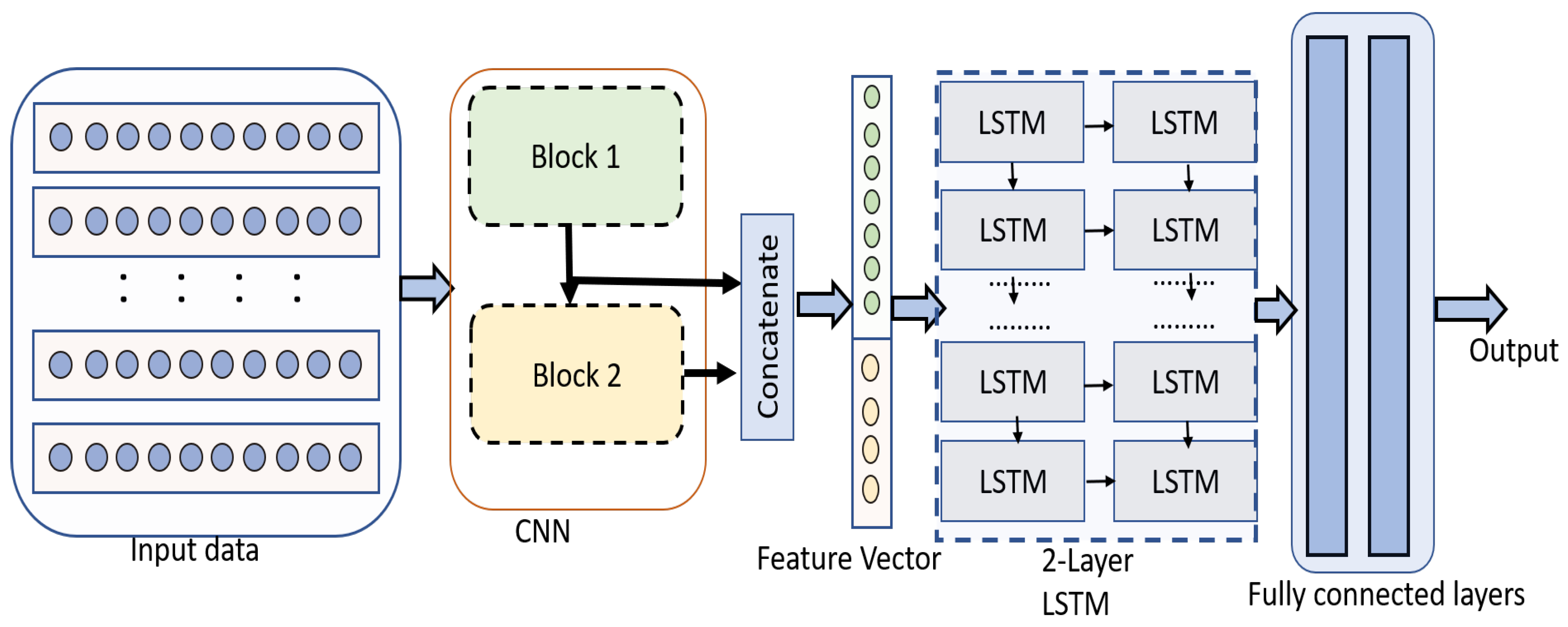
In this section, we discuss the details of the proposed framework. The purpose of this work is to design and develop a prediction model that can forecast the potential hotspots by employing sophisticated deep learning models. The pipeline of proposed framework is illustrated in Figure 1. As shown in Figure 1, the framework utilizes and exploits two deep learning models: (1) Convolutional Neural Network (CNN) and (2) Long-Short-Term-Memory (LSTM) Model. CNNs have the ability to extract hierarchical features that represent the generic representation of time-series data. On the other hand, LSTM models learn short and long-term dependencies from time series data. The goal of the proposed framework is to combine the advantages of both CNN and LSTM models. In the following sub-sections, we discuss the details of the proposed framework.
3.1. Data Pre-Processing
In this section, we discuss how to prepare the data for training the deep neural networks. In this work, we conduct analysis on the data collected from Center for Systems Science and Engineering (CSSE) at Johns Hopkins University (https://github.com/CSSEGISandData/COVID-19). The dataset contains daily statistics of the data related to number of positive cases, number of recoveries, and number of deaths. We observe that the dataset contains long sequences and training deep model with such long sequences cause following problems: (1) With such long sequences, the models take significant amount of time and require huge memory storage during training. (2) Back-propagating long sequences results in quick gradient vanishing that leads to poor learning of the model. Therefore, as a solution, we pre-process the data before feeding deep neural networks.
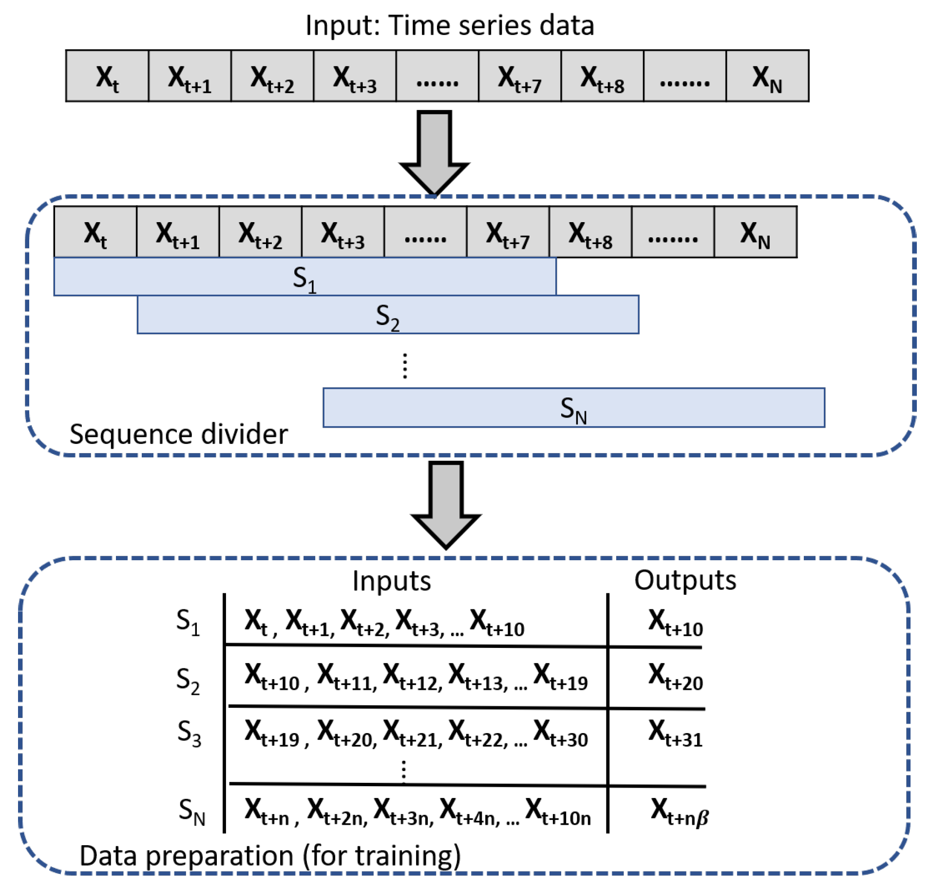
The overall process of data preparation is shown in Figure 2. As shown in the figure, we divide the long sequence into sub-sequences of fixed length, . In this paper, we set the value of to 10. Let S = represents long time series sequence over duration of T. We divide sequence S into a set of sub-sequences , where each sub-sequence contains the data of ten (since ) consecutive days. In the next step, we pre-process the data. Pre-processing step deals with cleaning the data from noise, account for missing data and normalization. Normalizing the data prevents the network nodes from saturation [39]. There are different types of normalization techniques that can be used for pre-processing [40]; however, in this work we use Min-Max normalization technique and formulated as in Equation (1).
where is the normalized value at time t, is the original value, and represent the minimum and maximum values over the range of data.
After normalization, we then prepare the data for training the CNN. The CNN takes the input data and maps a vector of past observations (provided as input) to output predictions. In order to train CNN using time-series data, the input sequence must be divided into a set of multiple examples. For this purpose, we re-arrange the data in each sub-sequence by dividing the sub-sequences into input and output patterns. For each sub-sequence , we sample its first ten data points as input and 10th data point is used as output for one-step prediction. After data preparation, we then provide data as input to the CNN for hierarchical features extraction.
3.2. Convolutional Neural Network
In this section section, we discuss the architecture of CNN used in proposed framework for feature extraction. Traditionally, the Multi-Layer Perceptron (MLP) model is widely adopted as feature extractor; however, it lost its popularity due to the following reason. The MLP model, due to dense connection of each perceptron to every other perceptron, is becoming redundant, inefficient and unscalable. CNN models address this problem by adopting a sparse connection of neurons in multiple layers. CNN is composed of multiple convolutional and pooling layers. Unlike MLP models, the neuron in each layer does not need to be connected to each and every neuron in the preceding layer. The neurons are connected only to a region of the input data and perform dot product operations on the input data according to certain filter size and stride. The size of filters and stride needs to be determined experimentally or using specific domain knowledge. These location invariant filters, learn specific patterns by allowing parameter and weight sharing, while slide over the data. Generally, neurons in each layer of CNN have certain weights and biases which is initialized and learned during the training process.
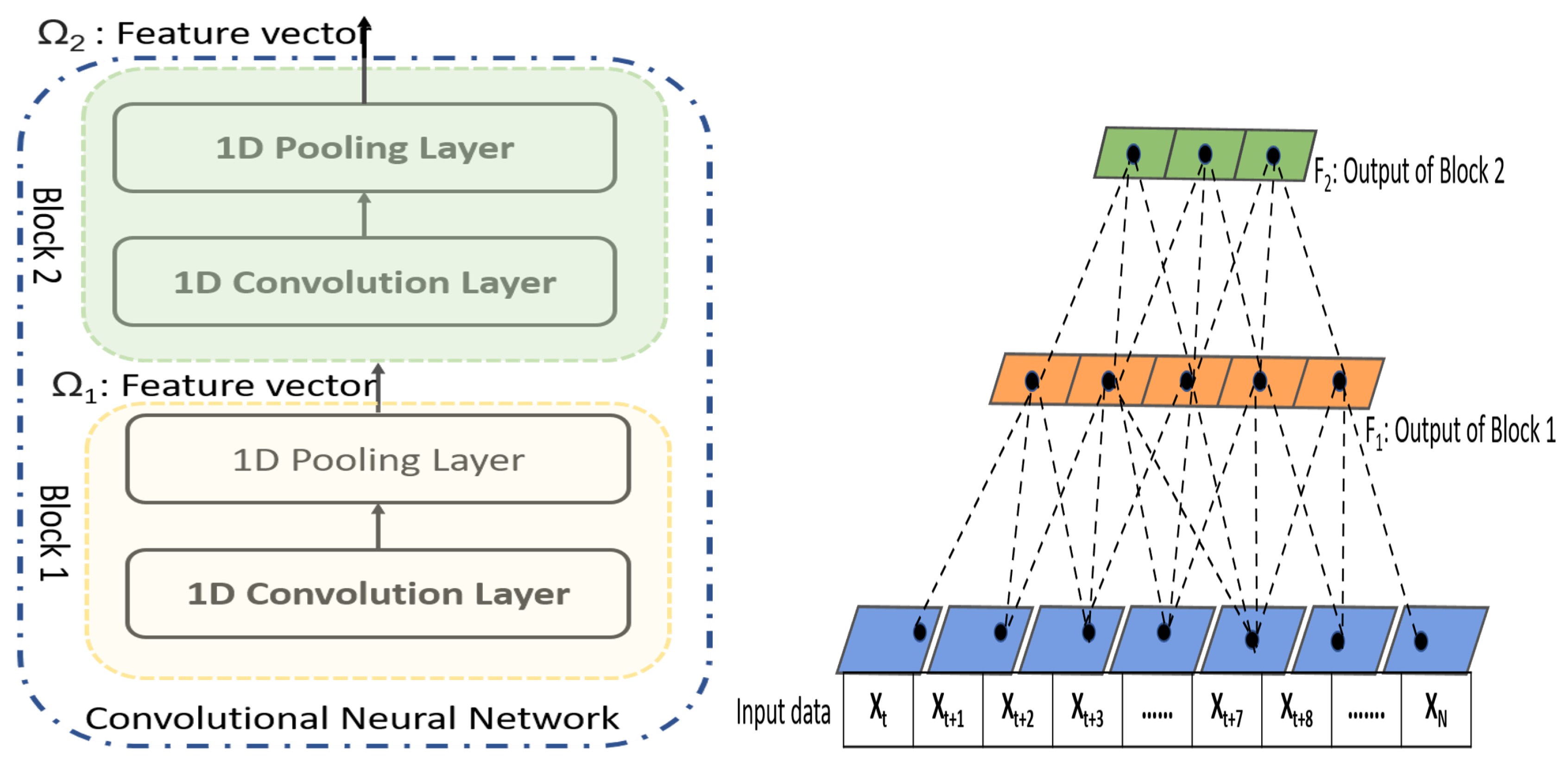
Admitting the success of CNN in feature extraction and classification tasks [41,42], we employ CNN for extracting morphological features of data. Our CNN is composed of two 1-D convolutional layers followed by two max pooing layers. This shallow architecture of CNN allows us to reduce the computational complexity during training and inference, and learns multiple time scale hierarchical features effectively. The architecture of the proposed CNN with two convolutional and two pooling layers is shown in Figure 3. We provide the details of each layer as follows:
1-D Convolutional layer performs the dot product of the time-series input data and convolution kernels. The convolutional layer depends on a number of parameters, including, number of filter , filter size and stride s. These parameters need to be determined before starting the training process. The convolution kernel can be viewed as a window that contains coefficients values in the form of a vector. During the forward pass, the windows slides over all the input data and provides a feature vector as an output. We can generate different feature vectors by applying convolution kernels of different sizes. In this way, we extract more useful information from the input data that ultimately enhances the performance of the CNN. The convolutional layer is always followed by a nonlinear activation function, namely Rectified Linear Unit (ReLU), that returns to zero if the input is negative and returns the value back if the input is positive. The activation function can be expressed as .
1-D Max-pooling layer employs a down sampling technique that reduces the size of the feature map obtained by convolution layers. The feature maps obtained by convolution layers are sensitive to the location of the features in the data. In order to make the feature vector more robust, a pooling layer is applied that extracts certain values from the feature vector obtained by covolutional layers. Similar to convolutional layers, pooling layers also employ a sliding window approach that takes a small portion of the input feature vector (equal to the size of windows) and takes the maximum or average value. In this way, the pooling layer produces a robust and summarized version of the feature map obtained by convolutional layers. Furthermore, the new feature map obtained by the pooling layer is translation invariant, since a small change in the input data will not affect the output values of the pooling layer.
Generally, our CNN network, shown in Figure 3, follows the architecture of [43] that consists of two blocks. The overall architecture of proposed CNN is illustrated in Figure 3a. As is obvious from the figure, each block consists of a set of one convolutional layer followed by one pooling layer. The convolutional layer of the first block contains 32 filters with size of 2. The convolutional layer of the second block contains 64 filter with size of 2. We use max-pooling in both blocks with size of 2. Let is a set of time-series sub-sequence applied as input to the CNN. The input is then passed through the first block and outputs a feature vector after passes through convolutional and pooling layer. The feature vector is then passed through a second block and produces feature vector .
The convolutional neural network achieved considerable success in predicting time series data [28,44,45]. These models use single time scale features from the last convolutional layer () to predict the sequences and do not incorporate multi-time scale features. Such a model performs well in long term prediction; however, the performance of these models degrades while predicting short or medium term data. To predict hotspots, it is useful to incorporate multiple time scale features. Since the dataset contains the data from different cities, where the number of positive cases is affected by many factors such as short and long duration interactions, physical proximity and environmental conditions. Due to these factors, populous cities have a high number of positive cases compare to less populous cities. From the empirical studies, we observe that using single time scale feature for small cities results in High Root Means Square Error (RMSE). Since we are using a single model for the prediction, instead of using single time scale feature, we employ a fusion strategy that fuses the features from both blocks. Feature vector and have different receptive fields that describe the input time-series data at different time scales. The difference between two feature vectors is described in Figure 3b. Each data point of feature vector describes a part of region of the original time-series data. Since the receptive fields of both blocks is different, therefore, feature vector and describes time-series data from different two different time scales. Furthermore, we also regarded the original input sequence as feature vector and represent it by . represents the feature vector of short time scale that reflects local changes in the data. We then employ the Long Short-Term Memory (LSTM) model to learn sequential or temporal dependencies of the features obtained by CNN.
3.3. Long Short-Term Memory
Long Short-Term Memory (LSTM) models are the special type of Recurrent Neural Networks (RNNs) which have the ability to learn long-term temporal or sequential dependencies due to feed back connections that causes internal memory. RNNs, due to the lack of memory mechanism, cannot perform well on long-term time series sequential data. This is due to the fact that RNN models utilize cyclic connections and suffer from the gradient vanishing or exploding problem. LSTM, on the other hand, solve the problem by using memory cells to store useful information and vanish undesired information, thus performs better than traditional RNNs. Each LSTM unit consists of a cell and each cell consists of three gates, i.e., input gate, forget gate, and output gate. With the help of these gates, the LSTM unit can control the flow of information by remembering important information and forgetting the unnecessary information. In this way, LSTM can capture temporal changes in sequential data and has been widely adopted in different problems.
To learn temporal dependencies at different time-scales, we concatenate feature vectors and and provide input to LSTM. We first describe the structure of LSTM cell and then show how we can build complete LSTM network by concatenating LSTM cells. Let = [0,1] represents a unit interval then = [−1,1]. The LSTM cell consists of two recurrent features, i.e., hidden state and current cell’s state at time t. At time t, output of the cell is a mathematical function of three values and expressed as in Equation (2).
where and represent hidden state and current state of the cell and , represent the previous hidden and previous state of the cell respectively. is the input time-series data provided as input at time t.
Inside the LSTM cell, hidden state and input time-series data d flow through three gates and update the current state of the cell using a sigmoid function, denoted by . Let , , and are the input, output and forget gates respectively. The output of each gate is a scalar value in the range of computed as follows.
The equation for input gate is calculated by:
The equation for output gate is calculated by:
The equation for forget gate is calculated by:
where are the weight vectors, are the biases. These weights and biases are learned during the training process. These gates behave like switches, where the gate is “ON” when its value is nearly 1 and “OFF” if value is nearly 0. Memory inside the cell is implemented by incorporating new information using input gate and remove unnecessary information using forget gate. New information is incorporated to the cell by using Equation (6)
where is the weight vector and , B are the biases.
The hidden state at time t is calculated as in Equation (8)
where ⊙ is the element-wise multiplication. All of above equations are implemented inside a single LSTM cell.
To design the LSTM layer, we simply concatenate m number of LSTM cells, i.e., , with each cell contains different set of weights and biases. We stack the individual weights and biases of all LSTM cells into a matrices. LSTM layer is evolved by applying activation functions in element-wise manner. The gate equations will now contain weight matrices, with size of that is compatible with the size of input data . Similarly, the dimensions of weights matrices, of hidden states will be and the size of biases, will be .
The final output provided by Equation (8) is regarded as the temporal dependencies learn by each LSTM and denoted by . The vector is then provided as input to a fully connected layer to provide the final prediction. The description of the CNN-LSTM framework is provided in Table 1 and the pipeline of the overall framework is illustrated in the figure.
4. Experiment Results
In this section, we discuss experimental results obtained using proposed method. We also demonstrate the effectiveness of proposed framework by comparing it with other state-of-the-art methods.
4.1. Experimental Data
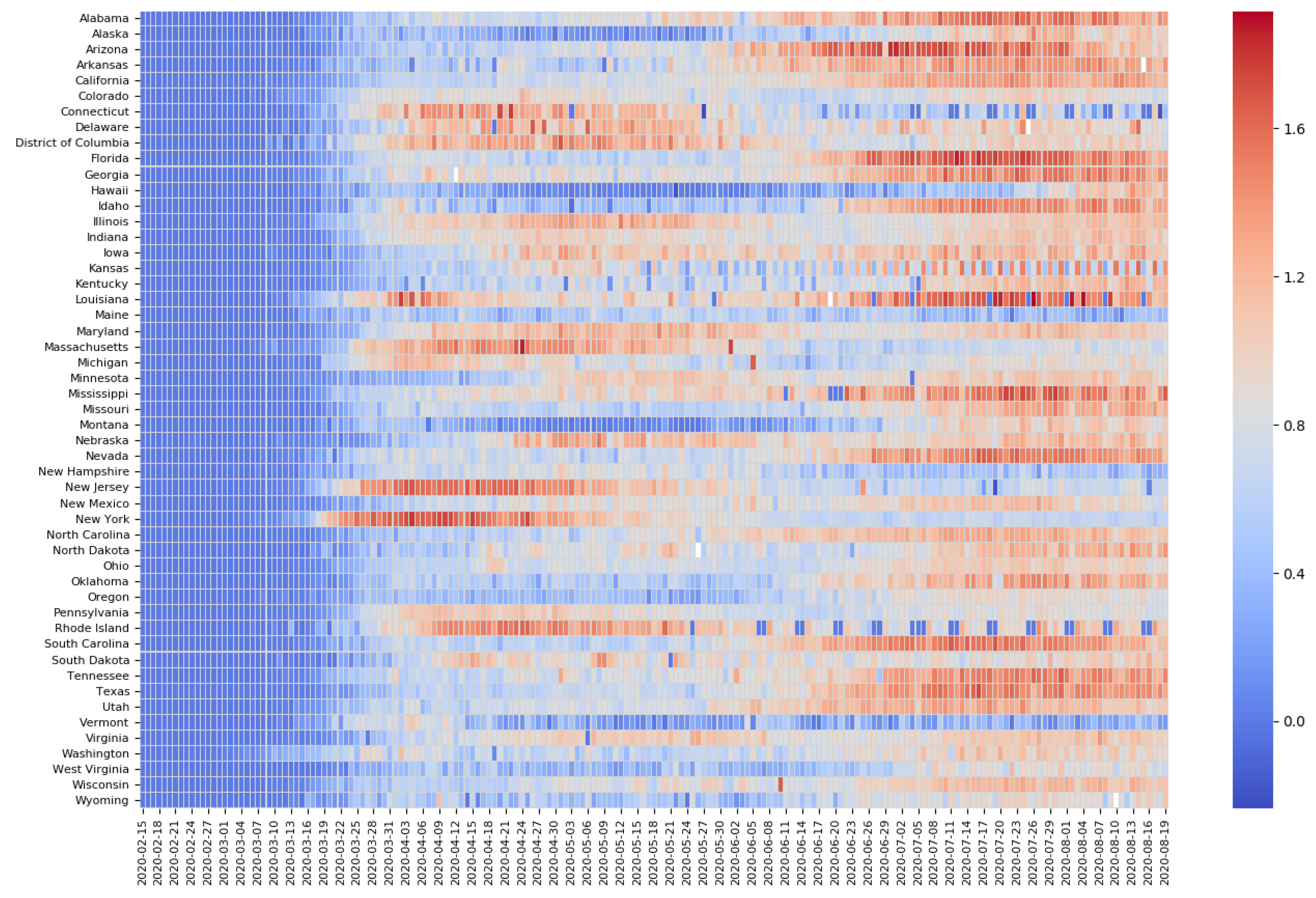
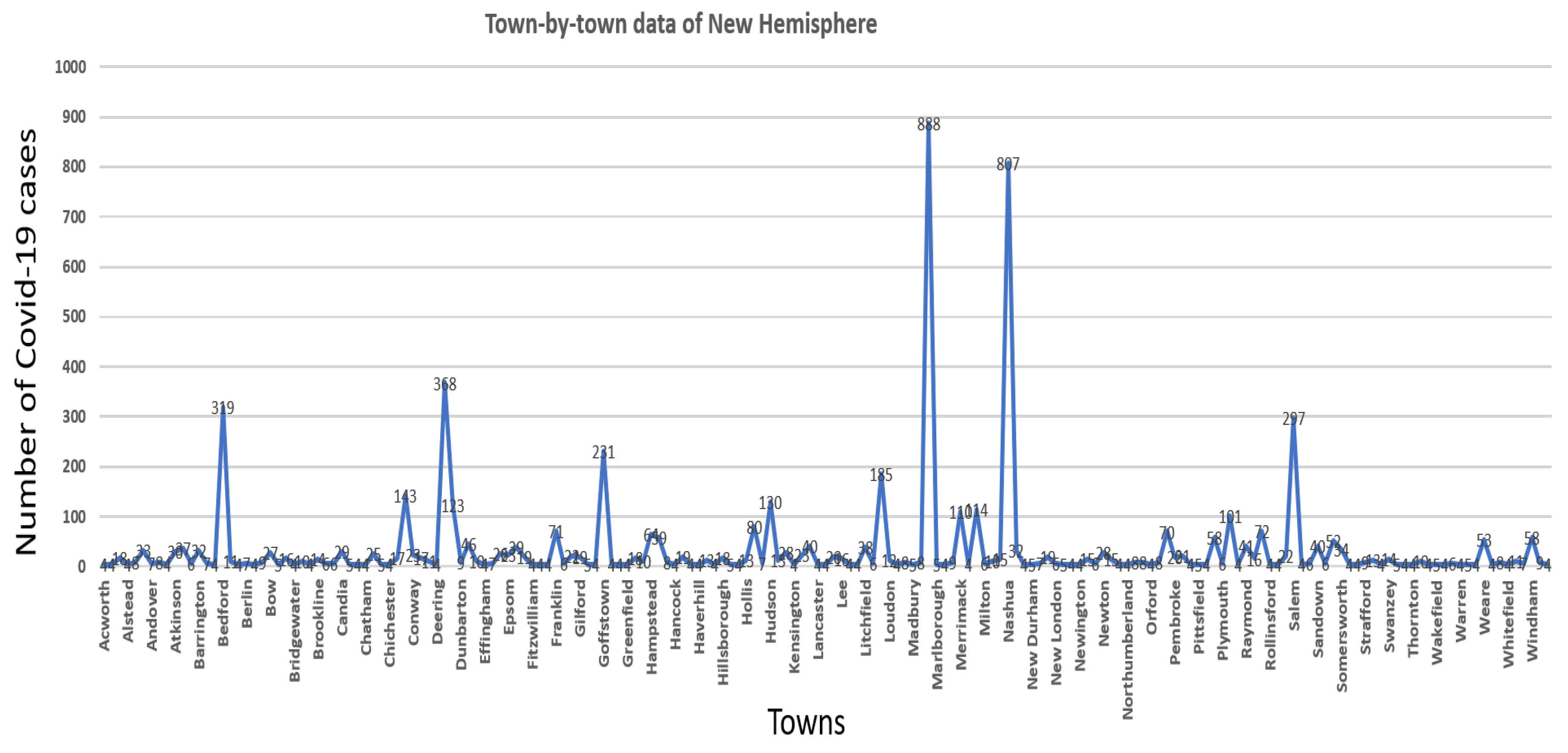
We perform experiments using the data collected and maintained by the Center for Systems Science and Engineering (CSSE) at Johns Hopkins University. The data is publicly available at (https://github.com/CSSEGISandData/COVID-19). The data refers to daily cumulative cases, deaths, recoveries starting from 22 January 2020 to date. In our study, we emphasise the significance of the total number of daily reported cases over a period of the last months. In our analysis, we use the data from United States due to the following easons. (1) In USA, the number of laboratory and clinically confirmed cases is increasing daily with a big margin compare to other countries. (2) The data also contains town-by-town data regarding the number of positive cases, which is vital for our analysis. Figure 4 illustrates the progression of COVID-19 positive cases over time in United States. The x-axis of the heat map shows the date starting from 15 February 2020 to 23 July 2020 with a step of three days gap. The y-axis shows state’s name of United states. Each cell in the heat map (encoded with colors) shows the number of new cases by state normalized by the population of each state. The blue color shows lower number of positive cases while the red color shows large number of positive cases. We also report data (number of COVID-19 positive cases) collected from 183 towns of New hampshire, asreported in Figure 5. The x-axis shows different town in New hemisphere and y-axis shows total number of positive cases in each town. The code at (https://github.com/JasonRBowling/covid19NewCasesPer100KHeatmap) is used to generate Figure 4.
After obtaining the data, we normalize the data as discussed in Section 3.1 before further processing. After data normalization, we form series of sequences that combine both historical data and target data.
The prediction horizon usually affects the accuracy of every predicting model. We first define the predicting horizon as the number of data points taken into consideration by a prediction model for predicting the next data point. In this paper, we fix the value of the predicting horizon to 10 days. In other words, we sample data points for 10 days and then predict the value on the 11th day.
We evaluate and compare proposed framework with other existing state-of-the-art predicting models. We group the methods into two categories: (1) Statistical models (2) Deep models. Statistical models include the Support Vector Regression (SVR) [46], Forward Feed-Forward Model [6,47,48,49], and Auto Regressive Integrated Moving Average (ARIMA) [48,50,51]. In a second category, we use different deep models, such as Long Short-term Memory (LSTM) [18,34], and Convolutional Neural Network (CNN) [28]. We briefly discuss each model as follows:
Performance Metrics: The performance of different time-series prediction models is evaluated by root-mean-square-error (RMSE) formulated as in Equation (9) and mean-absolute-error (MAE) formulated as in Equation (10).
where m is the number of predicted points, and represent actual and predicted value of ith points, respectively.
4.2. Hyper Parameters of CNN
We analyse the effect of number of filter and filter sizes of convolution layer on accuracy. There is no optimum way of determining these hyper parameters. Usually, these values are determined experimentally. The convolution filter captures the local features of the input data. Therefore, the filter size has an impact on their learning performance. If the filter size is too small, it cannot learn the contextual information of the input data. On the other hand, if the filter size is too large, it may loose local details of the input data. Furthermore, the number of filters also has an impact on accuracy. Using a smaller number of filters cannot capture enough features to perform the prediction task. The accuracy will increase with increase in the number of filter. However, too much filters may not increase the accuracy and also make the training computationally expensive. Table 1 shows the prediction performance (in terms of accuracy) using different filter sizes and number of filters. These values are selected randomly keeping in view the input size of data (10 data points/sequence in our case). From the table, it is obvious that filter size 2 and a large number of filters increase the accuracy.
4.3. Hyper Parameters of LSTM
Long short-term memory networks are widely used in different time-series forecasting problems, as mentioned before. However, the performances of these models are always influenced by different hyper parameters that need to be tuned to achieve better performance. The selection of these hyper parameters is not effortless and requires a sophisticated optimization method to find the optimized values of various hyper parameters. These hyper parameters include the depth of network, the number of units in hidden layers, and drop out ratio. In our experiments, we fix the number of units (100 in our case) and analyse the performance of the network by varying the number of layers. We trained three different network with different numbers of layers. The first network is trained with one layer, the second network is trained with two layers, and the third network is trained with three layers. The performance of all LSTMs is reported in Table 2. From the table, it is obvious that with constant number of units in all LSTMs, increasing the number of layers increases accuracy. From the experimental evidence, we observe that beats by a small margin; however, takes much time (almost double) during training. We also observe that also produces marginal results in some cases; however, it looses the generalization capability on validation data. Therefore, we observe a trade-off between number of layers and training efficiency.
4.4. Comparison of Results
In this section, we discuss and compare the performance of different methods with proposed framework. These state-of-the-art methods are employed for predicting different time-series problems. Due to the difference in dataset, model training and targets, these methods achieve different performance in different problem domains. For fair comparison, we carefully tune the different parameters of different models and select the version that performs best. The results are reported in Table 3. From the Table, it is obvious that proposed method beats other reference methods by a great margin.
Furthermore, we analyse the hotspot prediction performance of all models. For this purpose, we regard the prediction problem as a multi-class classification problem by analysing the increase or decrease in the number of cases with respect to the previous day for each regions/states. In more detail, prediction model takes the daily number of positive cases of the last ten days and predicts the number for the next day. To characterize the regions/states, we assign labels to each state/region as , where is the label of region/state i and n is total the number of regions/states. Let represents a set of times series data for n regions/states, where is regarded as ordered set of real values (representing the number cases per day) over the length of time series (10 days in our case) for region/state i.
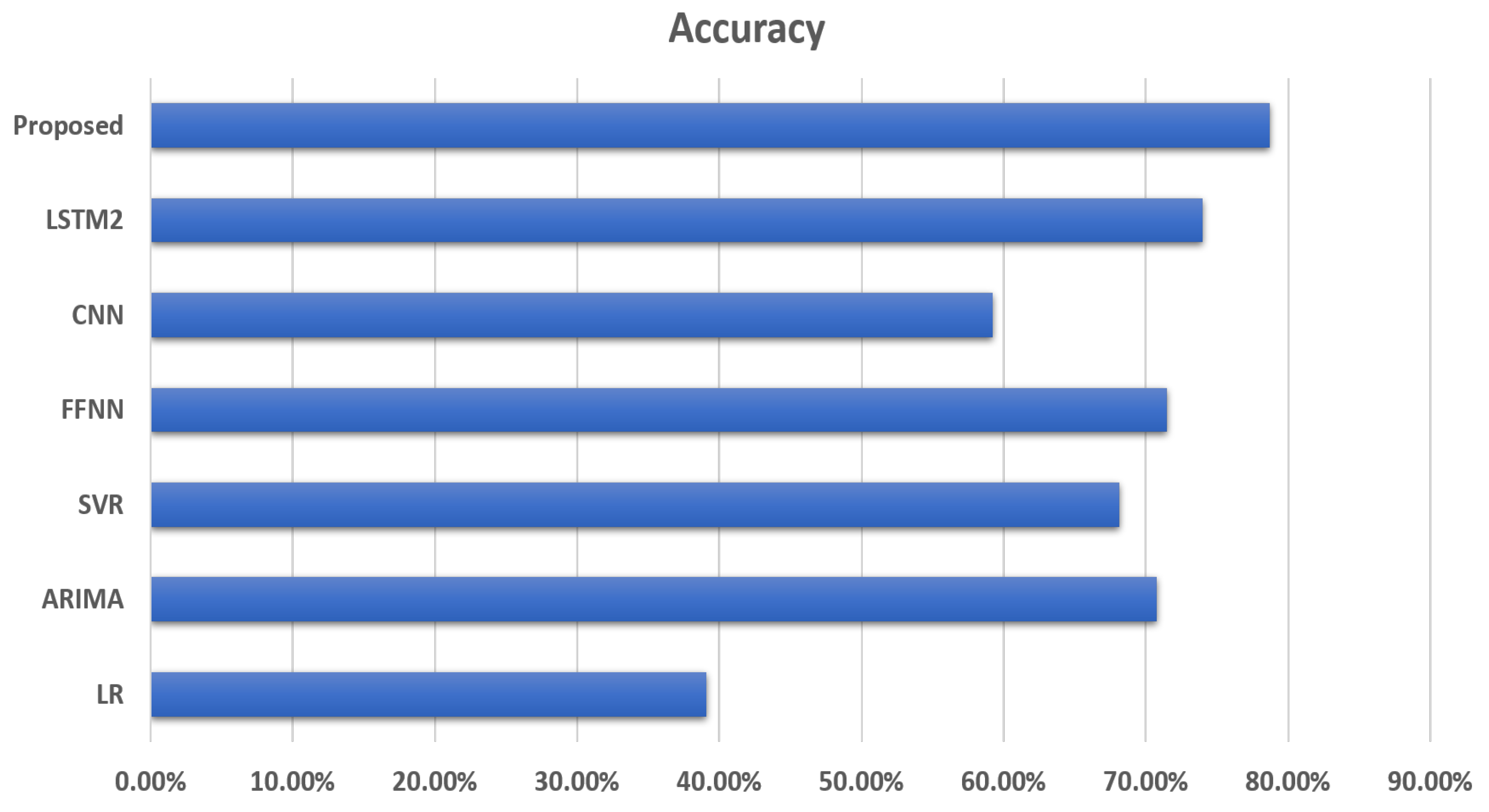
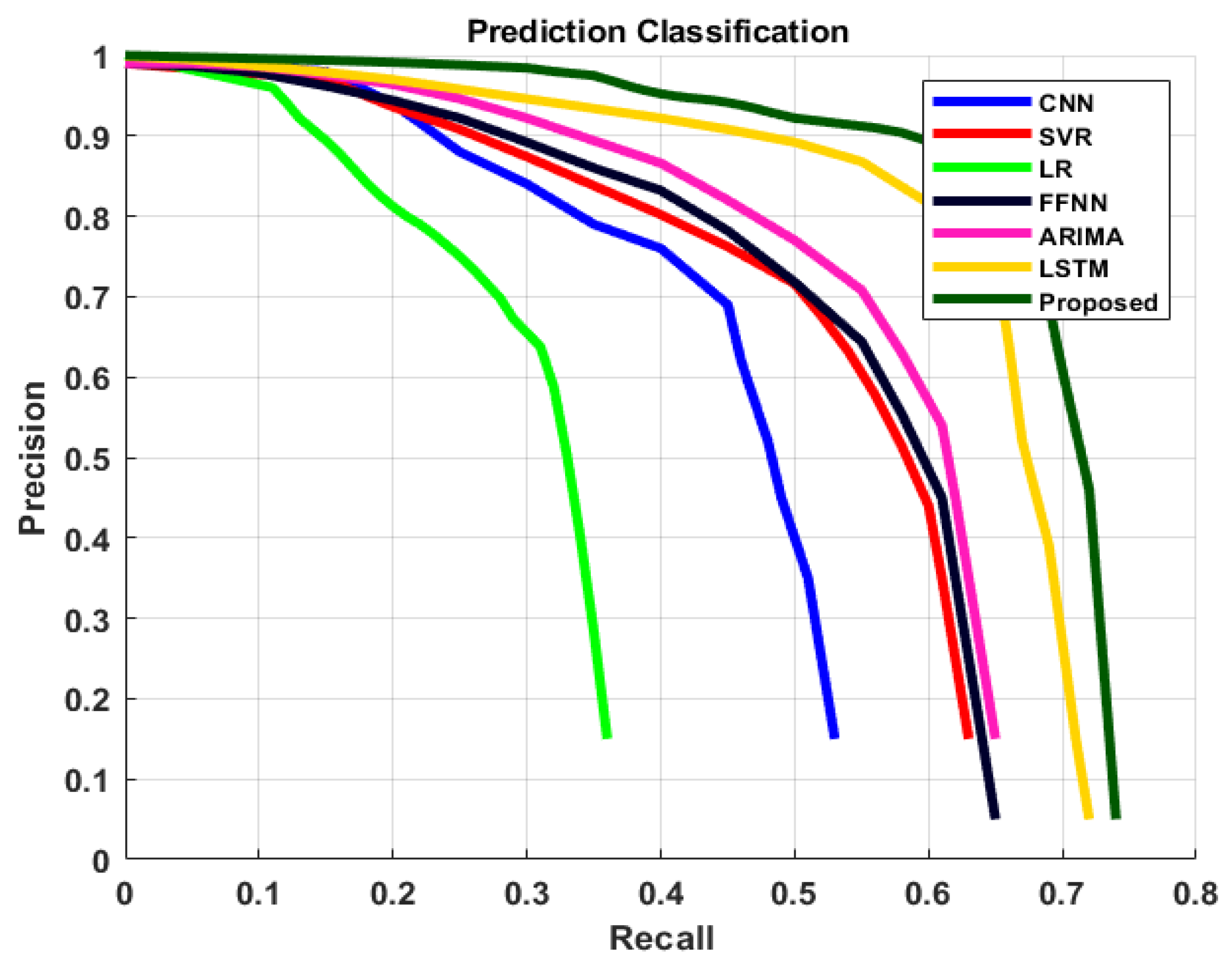
We provide X as input to each model and obtain set of predicted values , where each represents the number of cases in region/state i predicted by the model. Let is the collection of of inputs, outputs and labels. We then select top 10 labels by sorting the list Y in ascending order. We compute the following evaluation metric to compute the performance of each model. We follow the same convention in [3] to evaluate the performance of classifier using two metrics: (1) Accuracy, (2) area under the curve. The results are reported in Figure 6 and Figure 7. From the figures, it is obvious that the proposed method outperforms other state of the art methods.
4.5. Discussion
From the experiment results, it is obvious that proposed method outperforms other state-of-the-art methods. Among the reference models, Linear Regression (LR) performs relatively badly. This is due to fact that the LR model linearly approximates the target data. In other words, the LR model assumes a linear relationship between the forecast and predictor values. However, in our case, the relationship between the number of positive cases versus days is not linear. Furthermore, the LR model is susceptible to outliers. We also evaluate the performance of CNN model and the results using different evaluation metrics are reported in Table 3. From experiment results, it is obvious that CNN performs better than the LR model; however, it lags behind the other reference methods. This is because CNN models can not learn the temporal dependencies and not suitable for time-series prediction problems. SVR and ARIMA, and FFNN show similar performances in our case.
From the empirical studies, we observe that ARIMA and FFNN model achieve similar level of accuracy and produce lower MAE and RMSE values. This empirical evidence also validates the findings of [50,52]. However, the performance of ARIMA is better than FFNN in many time-series prediction problems, as reported in [51]. The LSTM model, on the other hand, beats all state-of-the-art methods. This is due to fact that the LSTM model learns temporal dependencies from the data and learn the context of observations over time by incorporating memory state. The proposed framework out-performs all reference methods by a significant margin. This is due to the fact that we combine the benefits of two deep neural networks, i.e., CNN and LSTM. The CNN model learns multi-time scale features from time-series data, which is then provided as input to LSTM. The LSTM then learns temporal dependencies from the features obtained by CNN. From the comparison results, we conclude that the proposed hybrid model that exploits features from different time scale performs better than other reference methods.
5. Conclusions
In this paper, we proposed a novel hybrid framework for the prediction of potential COVID-19 hotspots. The proposed framework has two sequential networks. The first network is the convolutional neural network that consists of two blocks with each block contains one covolutional layer followed by a pooling layer. The CNN network extract multi time-scale features from the input data. The multi time scales features extracted from two blocks are then concatenated and provided as input to LSTM model. The LSTM model then learns temporal dependencies. The proposed framework is evaluated and compared with different state-of-the-art forecasting models. From the experiment results, we demonstrated that the proposed framework outperforms other state-of-the-art models by a considerable margin. From aseries of experiment studies, we pointed out that LSTM models perform well and have been widely used in different forecasting problems since for a few years. However, we achieve a significant performance boost by utilizing the LSTM with CNN. However, the accuracy is still low. In our future work, we intend to integrate Meta-iPVP, Meta-i6mA, and HLPpred-Fuse predictors to further increase the performance. We believe that the proposed framework can easily be adopted in other time-series forecasting applications, for example, stock market prediction, weather prediction, earthquake prediction, gold price prediction, and other pandemic predictions.
Author Contributions
Conceptualization, S.D.K., L.A., and S.B.; methodology, S.D.K.; software, S.D.K.; validation, S.D.K., L.A.; formal analysis, S.D.K.; writing—original draft preparation, S.D.K.; writing—review and editing, S.D.K., L.A., and S.B.; visualization, S.D.K.; supervision, S.B.; project administration, S.B., and L.A.; funding acquisition, L.A. All authors have read and agreed to the published version of the manuscript.
Funding
This research received funding from King Abdulaziz City for Science and Technology (KACST), Kingdom of Saudi Arabia for the (COVID-19 Research Grant Program) under Grant no. 5-20-01-007-0006.
Acknowledgments
We acknowledge the support provided by King Abdulaziz City for Science and Technology (KACST), Kingdom of Saudi Arabia for the (COVID-19 Research Grant Program) under Grant no. 5-20-01-007-0006.
Conflicts of Interest
The authors have no conflict of interest.
References
- Karin, O.; Bar-On, Y.M.; Milo, T.; Katzir, I.; Mayo, A.; Korem, Y.; Dudovich, B.; Yashiv, E.; Zehavi, A.J.; Davidovich, N.; et al. Adaptive cyclic exit strategies from lockdown to suppress COVID-19 and allow economic activity. medRxiv 2020. [Google Scholar] [CrossRef] [Green Version]
- Nabipour, M.; Nayyeri, P.; Jabani, H.; Mosavi, A.; Salwana, E.; Shahab, S. Deep learning for stock market prediction. Entropy 2020, 22, 840. [Google Scholar] [CrossRef] [PubMed]
- Livieris, I.E.; Pintelas, E.; Pintelas, P. A CNN-LSTM model for gold price time-series forecasting. Neural Comput. Appl. 2020, 32, 17351–17360. [Google Scholar] [CrossRef]
- Wang, J.; Yu, L.C.; Lai, K.R.; Zhang, X. Dimensional sentiment analysis using a regional CNN-LSTM model. In Proceedings of the 54th Annual Meeting of the Association for Computational Linguistics (Volume 2: Short Papers), Berlin, Germany, 7–12 August 2016; pp. 225–230. [Google Scholar]
- Askari, M.; Askari, H. Time series grey system prediction-based models: Gold price forecasting. Trends Appl. Sci. Res. 2011, 6, 1287. [Google Scholar] [CrossRef]
- Guha, B.; Bandyopadhyay, G. Gold price forecasting using ARIMA model. J. Adv. Manag. Sci. 2016, 4, 117–121. [Google Scholar]
- Dubey, A.D. Gold price prediction using support vector regression and ANFIS models. In Proceedings of the 2016 International Conference on Computer Communication and Informatics (ICCCI), Coimbatore, India, 7–9 January 2016; pp. 1–6. [Google Scholar]
- Li, J.; Dai, Q.; Ye, R. A novel double incremental learning algorithm for time series prediction. Neural Comput. Appl. 2019, 31, 6055–6077. [Google Scholar] [CrossRef]
- Liu, D.; Li, Z. Gold price forecasting and related influence factors analysis based on random forest. In Proceedings of the Tenth International Conference on Management Science and Engineering Management, Baku, Azerbaijan, 30 August–2 September 2016; pp. 711–723. [Google Scholar]
- Makridou, G.; Atsalakis, G.S.; Zopounidis, C.; Andriosopoulos, K. Gold price forecasting with a neuro-fuzzy-based inference system. Int. J. Financ. Eng. Risk Manag. 2 2013, 1, 35–54. [Google Scholar] [CrossRef]
- Makridakis, S.; Spiliotis, E.; Assimakopoulos, V. Statistical and Machine Learning forecasting methods: Concerns and ways forward. PLoS ONE 2018, 13, e0194889. [Google Scholar] [CrossRef] [Green Version]
- Ai, Y.; Li, Z.; Gan, M.; Zhang, Y.; Yu, D.; Chen, W.; Ju, Y. A deep learning approach on short-term spatiotemporal distribution forecasting of dockless bike-sharing system. Neural Comput. Appl. 2019, 31, 1665–1677. [Google Scholar] [CrossRef]
- Zheng, J.; Fu, X.; Zhang, G. Research on exchange rate forecasting based on deep belief network. Neural Comput. Appl. 2019, 31, 573–582. [Google Scholar] [CrossRef]
- Zou, W.; Xia, Y. Back propagation bidirectional extreme learning machine for traffic flow time series prediction. Neural Comput. Appl. 2019, 31, 7401–7414. [Google Scholar] [CrossRef]
- Chang, L.C.; Chen, P.A.; Chang, F.J. Reinforced two-step-ahead weight adjustment technique for online training of recurrent neural networks. IEEE Trans. Neural Networks Learn. Syst. 2012, 23, 1269–1278. [Google Scholar] [CrossRef] [PubMed]
- ur Sami, I.; Junejo, K.N. Predicting Future Gold Rates using Machine Learning Approach. Int. J. Adv. Comput. Sci. Appl. 2017, 8, 92–99. [Google Scholar]
- Chung, J.; Gulcehre, C.; Cho, K.; Bengio, Y. Empirical evaluation of gated recurrent neural networks on sequence modeling. arXiv 2014, arXiv:1412.3555. [Google Scholar]
- Lipton, Z.C.; Kale, D.C.; Elkan, C.; Wetzel, R. Learning to diagnose with LSTM recurrent neural networks. arXiv 2015, arXiv:1511.03677. [Google Scholar]
- Donahue, J.; Anne Hendricks, L.; Guadarrama, S.; Rohrbach, M.; Venugopalan, S.; Saenko, K.; Darrell, T. Long-term recurrent convolutional networks for visual recognition and description. In Proceedings of the IEEE Conference on Computer Vision and Pattern Recognition, Boston, MA, USA, 7–12 June 2015; pp. 2625–2634. [Google Scholar]
- Punia, S.; Nikolopoulos, K.; Singh, S.P.; Madaan, J.K.; Litsiou, K. Deep learning with long short-term memory networks and random forests for demand forecasting in multi-channel retail. Int. J. Prod. Res. 2020, 58, 4964–4979. [Google Scholar] [CrossRef]
- Bao, W.; Yue, J.; Rao, Y. A deep learning framework for financial time series using stacked autoencoders and long-short term memory. PLoS ONE 2017, 12, e0180944. [Google Scholar] [CrossRef] [Green Version]
- Sirignano, J.; Cont, R. Universal features of price formation in financial markets: Perspectives from deep learning. Quant. Financ. 2019, 19, 1449–1459. [Google Scholar] [CrossRef]
- Tsantekidis, A.; Passalis, N.; Tefas, A.; Kanniainen, J.; Gabbouj, M.; Iosifidis, A. Using deep learning to detect price change indications in financial markets. In Proceedings of the 2017 25th European Signal Processing Conference (EUSIPCO), Kos, Greece, 28 August–2 September 2017; pp. 2511–2515. [Google Scholar]
- Huang, J.; Kingsbury, B. Audio-visual deep learning for noise robust speech recognition. In Proceedings of the 2013 IEEE International Conference on Acoustics, Speech and Signal Processing, Vancouver, BC, Canada, 26–31 May 2013; pp. 7596–7599. [Google Scholar]
- Krizhevsky, A.; Sutskever, I.; Hinton, G.E. Imagenet classification with deep convolutional neural networks. In Proceedings of the Advances in Neural Information Processing Systems, Lake Tahoe, NV, USA, 3–6 December 2012; pp. 1097–1105. [Google Scholar]
- Garcia-Garcia, A.; Orts-Escolano, S.; Oprea, S.; Villena-Martinez, V.; Garcia-Rodriguez, J. A review on deep learning techniques applied to semantic segmentation. arXiv 2017, arXiv:1704.06857. [Google Scholar]
- Girshick, R.; Donahue, J.; Darrell, T.; Malik, J. Rich feature hierarchies for accurate object detection and semantic segmentation. In Proceedings of the IEEE Conference on Computer Vision and Pattern Recognition, Columbus, OH, USA, 23–28 June 2014; pp. 580–587. [Google Scholar]
- Zhao, B.; Lu, H.; Chen, S.; Liu, J.; Wu, D. Convolutional neural networks for time series classification. J. Syst. Eng. Electron. 2017, 28, 162–169. [Google Scholar] [CrossRef]
- Chen, C.T.; Chen, A.P.; Huang, S.H. Cloning strategies from trading records using agent-based reinforcement learning algorithm. In Proceedings of the 2018 IEEE International Conference on Agents (ICA), Singapore, 28–31 July 2018; pp. 34–37. [Google Scholar]
- Sezer, O.B.; Ozbayoglu, A.M. Algorithmic financial trading with deep convolutional neural networks: Time series to image conversion approach. Appl. Soft Comput. 2018, 70, 525–538. [Google Scholar] [CrossRef]
- Sainath, T.N.; Vinyals, O.; Senior, A.; Sak, H. Convolutional, long short-term memory, fully connected deep neural networks. In Proceedings of the 2015 IEEE International Conference on Acoustics, Speech and Signal Processing (ICASSP), Brisbane, QLD, Australia, 19–24 April 2015; pp. 4580–4584. [Google Scholar]
- Li, C.; Wang, P.; Wang, S.; Hou, Y.; Li, W. Skeleton-based action recognition using LSTM and CNN. In Proceedings of the 2017 IEEE International Conference on Multimedia & Expo Workshops (ICMEW), Hong Kong, China, 10–14 July 2017; pp. 585–590. [Google Scholar]
- Zhao, Y.; Yang, R.; Chevalier, G.; Xu, X.; Zhang, Z. Deep residual bidir-LSTM for human activity recognition using wearable sensors. Math. Probl. Eng. 2018, 2018, 1–13. [Google Scholar] [CrossRef]
- Kim, C.; Li, F.; Rehg, J.M. Multi-object tracking with neural gating using bilinear lstm. In Proceedings of the European Conference on Computer Vision (ECCV), Munich, Germany, 8–14 September 2018; pp. 200–215. [Google Scholar]
- Kim, T.Y.; Cho, S.B. Predicting residential energy consumption using CNN-LSTM neural networks. Energy 2019, 182, 72–81. [Google Scholar] [CrossRef]
- Du, S.; Li, T.; Gong, X.; Yang, Y.; Horng, S.J. Traffic flow forecasting based on hybrid deep learning framework. In Proceedings of the 2017 12th International Conference on Intelligent Systems and Knowledge Engineering (ISKE), Nanjing, China, 24–26 November 2017; pp. 1–6. [Google Scholar]
- Lin, T.; Guo, T.; Aberer, K. Hybrid neural networks for learning the trend in time series. In Proceedings of the Twenty-Sixth International Joint Conference on Artificial Intelligence, Melbourne, Australia, 19–25 August 2017; pp. 2273–2279. [Google Scholar]
- Xue, N.; Triguero, I.; Figueredo, G.P.; Landa-Silva, D. Evolving Deep CNN-LSTMs for Inventory Time Series Prediction. In Proceedings of the 2019 IEEE Congress on Evolutionary Computation (CEC), Wellington, New Zealand, 10–13 June 2019; pp. 1517–1524. [Google Scholar]
- Kitapcı, O.; Özekicioğlu, H.; Kaynar, O.; Taştan, S. The effect of economic policies applied in Turkey to the sale of automobiles: Multiple regression and neural network analysis. Procedia-Soc. Behav. Sci. 2014, 148, 653–661. [Google Scholar] [CrossRef] [Green Version]
- Kheirkhah, A.; Azadeh, A.; Saberi, M.; Azaron, A.; Shakouri, H. Improved estimation of electricity demand function by using of artificial neural network, principal component analysis and data envelopment analysis. Comput. Ind. Eng. 2013, 64, 425–441. [Google Scholar] [CrossRef]
- Yamashita, R.; Nishio, M.; Do, R.K.G.; Togashi, K. Convolutional neural networks: An overview and application in radiology. Insights Imaging 2018, 9, 611–629. [Google Scholar] [CrossRef] [Green Version]
- Tajbakhsh, N.; Shin, J.Y.; Gurudu, S.R.; Hurst, R.T.; Kendall, C.B.; Gotway, M.B.; Liang, J. Convolutional neural networks for medical image analysis: Full training or fine tuning? IEEE Trans. Med Imaging 2016, 35, 1299–1312. [Google Scholar] [CrossRef] [Green Version]
- Hao, Y.; Gao, Q. Predicting the Trend of Stock Market Index Using the Hybrid Neural Network Based on Multiple Time Scale Feature Learning. Appl. Sci. 2020, 10, 3961. [Google Scholar] [CrossRef]
- Acharya, U.R.; Oh, S.L.; Hagiwara, Y.; Tan, J.H.; Adam, M.; Gertych, A.; San Tan, R. A deep convolutional neural network model to classify heartbeats. Comput. Biol. Med. 2017, 89, 389–396. [Google Scholar] [CrossRef]
- Fawaz, H.I.; Forestier, G.; Weber, J.; Idoumghar, L.; Muller, P.A. Deep neural network ensembles for time series classification. In Proceedings of the 2019 International Joint Conference on Neural Networks (IJCNN), Budapest, Hungary, 14–19 July 2019; pp. 1–6. [Google Scholar]
- Ju, X.; Cheng, M.; Xia, Y.; Quo, F.; Tian, Y. Support Vector Regression and Time Series Analysis for the Forecasting of Bayannur’s Total Water Requirement; ITQM: San Rafael, Ecuador, 2014; pp. 523–531. [Google Scholar]
- Fattah, J.; Ezzine, L.; Aman, Z.; El Moussami, H.; Lachhab, A. Forecasting of demand using ARIMA model. Int. J. Eng. Bus. Manag. 2018, 10, 1847979018808673. [Google Scholar] [CrossRef] [Green Version]
- Liu, Q.; Liu, X.; Jiang, B.; Yang, W. Forecasting incidence of hemorrhagic fever with renal syndrome in China using ARIMA model. BMC Infect. Dis. 2011, 11, 218. [Google Scholar] [CrossRef] [PubMed] [Green Version]
- Nichiforov, C.; Stamatescu, I.; Făgărăşan, I.; Stamatescu, G. Energy consumption forecasting using ARIMA and neural network models. In Proceedings of the 2017 5th International Symposium on Electrical and Electronics Engineering (ISEEE), Galati, Romania, 20–22 October 2017; pp. 1–4. [Google Scholar]
- Adebiyi, A.A.; Adewumi, A.O.; Ayo, C.K. Comparison of ARIMA and artificial neural networks models for stock price prediction. J. Appl. Math. 2014, 2014, 1–7. [Google Scholar] [CrossRef] [Green Version]
- Merh, N.; Saxena, V.P.; Pardasani, K.R. A comparison between hybrid approaches of ANN and ARIMA for Indian stock trend forecasting. Bus. Intell. J. 2010, 3, 23–43. [Google Scholar]
- Sterba, J.; Hilovska, K. The implementation of hybrid ARIMA neural network prediction model for aggregate water consumption prediction. Aplimat J. Appl. Math. 2010, 3, 123–131. [Google Scholar]
Figure 1.
Pipeline of proposed framework.

Figure 2.
Pipeline of data preparation and normalization.

Figure 3.
Figure on right side shows the proposed Convolutional Neural Network (CNN) used in our framework. The CNN consists of two blocks. From each block we extract multi time-scale features as illustrated in the figure on the left.
Figure 3.
Figure on right side shows the proposed Convolutional Neural Network (CNN) used in our framework. The CNN consists of two blocks. From each block we extract multi time-scale features as illustrated in the figure on the left.

Figure 4.
A heat map, where different colour codes represent different the number of COVID-19 positive cases normalized by the state’s population. The more red the color, the higher the number of cases at a particular time and state.
Figure 4.
A heat map, where different colour codes represent different the number of COVID-19 positive cases normalized by the state’s population. The more red the color, the higher the number of cases at a particular time and state.

Figure 5.
Town-by-town data of New Hampshire in a single day. The data regarding the number of positive cases is collected from 183 towns of the state.
Figure 5.
Town-by-town data of New Hampshire in a single day. The data regarding the number of positive cases is collected from 183 towns of the state.

Figure 6.
Performance comparison of different methods in terms of accuracy.

Figure 7.
Performance comparison of different methods in terms of precision recall curves.


Table 1.
Effect of filter sizes and number of filters on the performance of Convolutional Neural Network (CNN).
Table 1.
Effect of filter sizes and number of filters on the performance of Convolutional Neural Network (CNN).
| Convolutional Neural Network | ||||
|---|---|---|---|---|
| Layer-1 | Layer-2 | |||
| Filter Size | # of Filters | Filter Size | # of Filters | Accuracy |
| 2 | 5 | 3 | 7 | 0.64 |
| 3 | 10 | 4 | 15 | 0.57 |
| 5 | 20 | 6 | 25 | 0.43 |
| 6 | 25 | 3 | 30 | 0.39 |
| 2 | 32 | 2 | 64 | 0.74 |
Table 2.
Performance of different LSTM models with different number of layers and number of units remains constant (100).
Table 2.
Performance of different LSTM models with different number of layers and number of units remains constant (100).
| Number of Layers | Training Time (s) | Accuracy | |
|---|---|---|---|
| LSTM_1 | 1 | 350 | 0.64% |
| LSTM_2 | 2 | 795 | 0.72% |
| LSTM_3 | 3 | 1587 | 0.73% |
Table 3.
Comparison of different forecasting methods. The performance is evaluated in term of Mean Absolute Error (MAE), and Root Mean Square Error (RMSE). For MAE and RMSE values, lower is better.
Table 3.
Comparison of different forecasting methods. The performance is evaluated in term of Mean Absolute Error (MAE), and Root Mean Square Error (RMSE). For MAE and RMSE values, lower is better.
| Metrics | Models | ||||||
|---|---|---|---|---|---|---|---|
| LR | SVR | ARIMA | FFNN | CNN | LSTM | Proposed | |
| MAE | 476.41 | 310.23 | 201.75 | 115.03 | 276.95 | 120.76 | 74.27 |
| RMSE | 580.43 | 414.63 | 283.46 | 167.25 | 386.92 | 179.41 | 106.90 |
Publisher’s Note: MDPI stays neutral with regard to jurisdictional claims in published maps and institutional affiliations. |
© 2020 by the authors. Licensee MDPI, Basel, Switzerland. This article is an open access article distributed under the terms and conditions of the Creative Commons Attribution (CC BY) license (http://creativecommons.org/licenses/by/4.0/).
Share and Cite
MDPI and ACS Style
Khan, S.D.; Alarabi, L.; Basalamah, S. Toward Smart Lockdown: A Novel Approach for COVID-19 Hotspots Prediction Using a Deep Hybrid Neural Network. Computers 2020, 9, 99. https://0-doi-org.brum.beds.ac.uk/10.3390/computers9040099
AMA Style
Khan SD, Alarabi L, Basalamah S. Toward Smart Lockdown: A Novel Approach for COVID-19 Hotspots Prediction Using a Deep Hybrid Neural Network. Computers. 2020; 9(4):99. https://0-doi-org.brum.beds.ac.uk/10.3390/computers9040099
Chicago/Turabian StyleKhan, Sultan Daud, Louai Alarabi, and Saleh Basalamah. 2020. "Toward Smart Lockdown: A Novel Approach for COVID-19 Hotspots Prediction Using a Deep Hybrid Neural Network" Computers 9, no. 4: 99. https://0-doi-org.brum.beds.ac.uk/10.3390/computers9040099
Note that from the first issue of 2016, this journal uses article numbers instead of page numbers. See further details here.