Backward Induction versus Forward Induction Reasoning

Abstract

In this paper we want to shed some light on what we mean by backward induction and forward induction reasoning in dynamic games. To that purpose, we take the concepts of common belief in future rationality (Perea [1]) and extensive form rationalizability (Pearce [2], Battigalli [3], Battigalli and Siniscalchi [4]) as possible representatives for backward induction and forward induction reasoning. We compare both concepts on a conceptual, epistemic and an algorithm level, thereby highlighting some of the crucial differences between backward and forward induction reasoning in dynamic games.

1. Introduction

The ideas of backward induction and forward induction play a prominent role in the literature on dynamic games. Often, terms like backward and forward induction reasoning, and backward and forward induction concepts, are used to describe a particular pattern of reasoning in such games. But what exactly do we mean by backward induction and forward induction?

The literature offers no precise answer here. Only for the class of dynamic games with perfect information there is a clear definition of backward induction (based on Zermelo [5]), but otherwise there is no consensus on how to precisely formalize backward and forward induction. In fact, various authors have presented their own, personal interpretation of these two ideas. Despite this variety, there seems to be a common message in the authors’ definitions of backward and forward induction, which can be described as follows:

• Backward induction represents a pattern of reasoning in which a player, at every stage of the game, only reasons about the opponents’ future behavior and beliefs, and not about choices that have been made in the past. So, he takes the opponents’ past choices for granted, but does not draw any new conclusions from these.
• In contrast, forward induction requires a player, at every stage, to think critically about the observed past choices by his opponents. He should always try to find a plausible reason for why his opponents have made precisely these choices in the past, and he should use this to possibly reconsider his belief about the opponents’ future, present, and unobserved past choices.

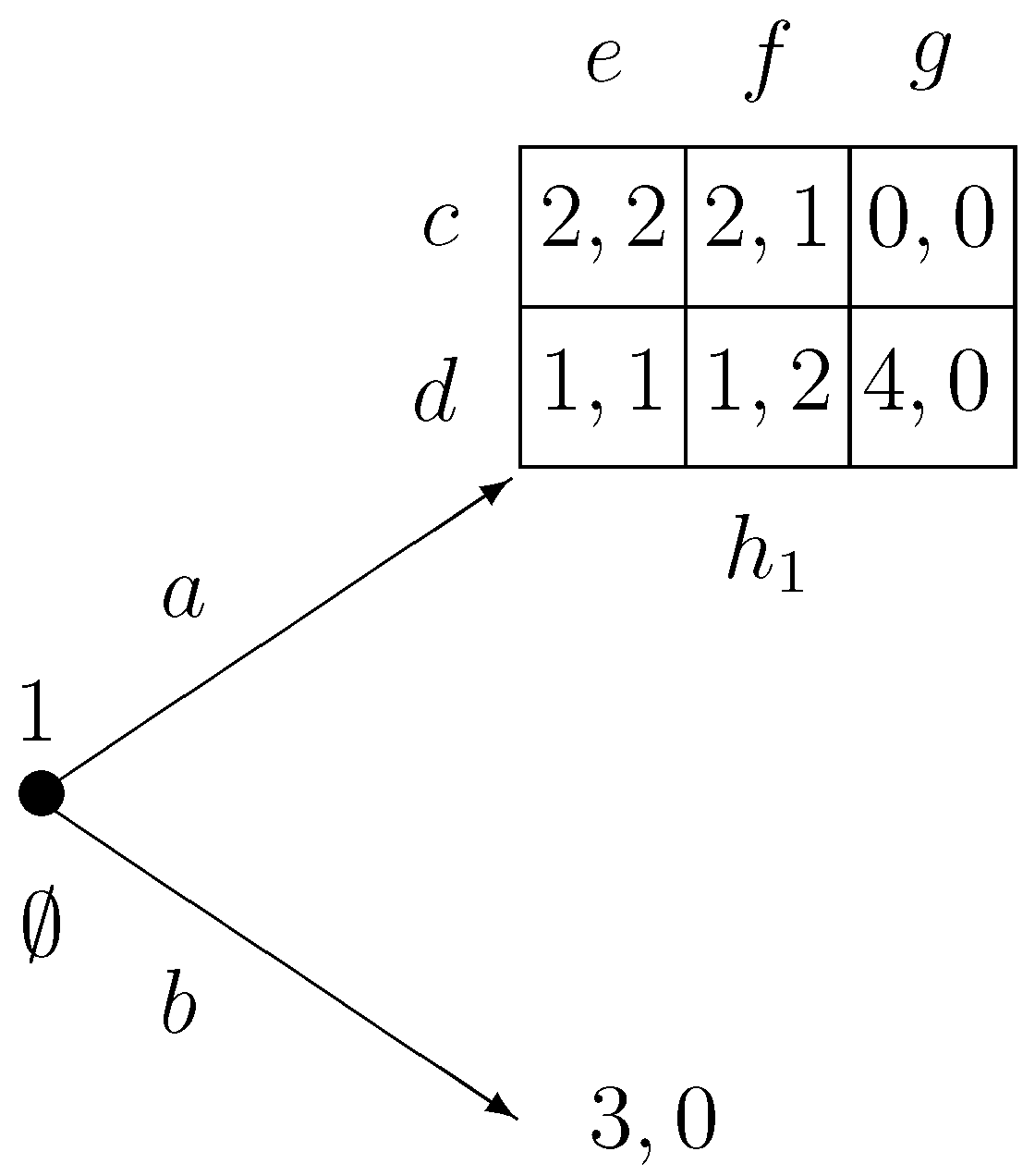
In order to illustrate these two ideas, let us consider the game in Figure 1. So, at the beginning of the game, ∅, player 1 chooses between a and $b.$ If he chooses $b,$ the game ends and the players’ utilities are 3 and $0.$ If he chooses $a,$ the game moves to information set $h_1$ where players 1 and 2 simultaneously choose from $\{c,d\}$ and $\{e,f,g\}$ respectively.

Figure 1. Backwards induction and forward induction may lead to opposite choices.

Figure 1. Backwards induction and forward induction may lead to opposite choices.

If player 1 believes that player 2 chooses rationally, then he anticipates that player 2 will not choose $g,$ and will therefore choose b at the beginning. But suppose now that the game actually reaches $h_1,$ and that player 2 must make a choice there. What should player 2 believe or do at $h_1?$

According to backward induction, player 2 should at $h_1$ only reason about player 1’s behavior and beliefs at $h_1,$ and take his past choice a for granted. In that case, it is reasonable for player 2 to believe that player 1 still believes that player 2 will not choose $g.$ Hence, player 2 will expect player 1 to choose c at $h_1,$ and player 2 would thus go for strategy $e.$

According to forward induction, player 2 should at $h_1$ try to make sense of player 1’s past choice $a.$ So, what reason could player 1 have to choose $a,$ and not $b,$ at the beginning? The only plausible reason could be that player 1 actually believed that player 2, with sufficiently high probability, would choose $g.$ But if that were the case, then player 2 must conclude at $h_1$ that player 1 will choose d there, since that is his only chance to obtain more than 3. So, player 2 should then go for $f,$ and not $e.$

So we see that backward and forward induction lead to opposite choices for player 2 in this game: backward induction leads to $e,$ whereas forward induction leads to $f.$ The crucial difference between the two ideas is that under backward induction, player 2 should at $h_1$ not draw any new conclusions from player 1’s past choice a. Under forward induction, player 2 should at $h_1$ use player 1’s past choice a to form a new belief about player 1, namely that he believes that player 2 will (with sufficiently high probability) go for $g.$

Up to this stage we have only given some very broad, and rather unprecise, descriptions of backward and forward induction. Sometimes such descriptions are enough to analyze a game, like the one in Figure 1, but for other games it may be necessary to have a precise description of these two ideas, or to have them incorporated formally in some concept.

The literature actually offers a broad spectrum of formal concepts—most of these being equilibrium concepts—that incorporate the ideas of backward and forward induction. Historically, the equilibrium concept of sequential equilibrium (Kreps and Wilson [6]) is regarded as an important backward induction concept. Its main condition, sequential rationality, states that a player, at every stage, should believe that his opponents will make optimal choices at present and future information sets, given their beliefs there. No strategic conditions are imposed on beliefs about the opponents’ past behavior. As such, sequential equilibrium only requires a player to reason about his opponents’ future behavior, and may therefore be seen as a backward induction concept.

A problem with this concept, however, is that it incorporates an equilibrium condition which is hard to justify if the game is only played once, especially when there is no communication between the players before the game starts (see Bernheim [7] for a similar critique to Nash equilibrium). The equilibrium condition entails that a player believes that his opponents are correct about his own beliefs, and that he believes that two different players share the same belief about an opponent’s future behavior. Aumann and Brandenburger [8], Asheim [9] and Perea [10] discuss similar conditions that lead to Nash equilibrium. Another drawback of the sequential equilibrium concept—and this is partially due to the equilibrium condition—is that the backward induction reasoning is somewhat hidden in the definition of sequential equilibrium, and not explicitly formulated as such.

In contrast, a backward induction concept that does not impose such equilibrium conditions, and which is very explicit about the backward induction reasoning being used, is common belief in future rationality (Perea [1]). It is a belief-based concept which states that a player should always believe that his opponents will choose rationally now and in the future, that a player always believes that every opponent always believes that his opponents will choose rationally now and in the future, and so on. No other conditions are imposed. The concept is closely related to sequential rationalizability (Dekel, Fudenberg and Levine [11,12] and Asheim and Perea [13]) and to backwards rationalizability (Penta [14]). (See Perea [1] for more details on this). Moreover, sequential equilibrium constitutes a refinement of common belief in future rationality, the main difference being the equilibrium condition that sequential equilibrium additionally imposes. In a sense, common belief in future rationality can be regarded as a backward induction concept that is similar to, but more basic and transparent than, sequential equilibrium. It can therefore serve as a basic representative of the idea of backward induction in general dynamic games, and we will use it as such in this paper.

Let us now turn to forward induction reasoning. In the 1980’s and 1990’s, forward induction has traditionally be modeled by equilibrium refinements. Some of these have been formulated as refinements of sequential equilibrium, by restricting the players’ beliefs about the opponents’ past behavior as well. Examples are justifiable sequential equilibrium (McLennan [15]), forward induction equilibrium (Cho [16]) and stable sets of beliefs (Hillas [17]) for general dynamic games, and the intuitive criterion (Cho and Kreps [18]) and its various refinements for signaling games. By doing so, these authors have actually been incorporating a forward induction argument inside a backward induction concept, namely sequential equilibrium. So in a sense we are combining backward induction and forward induction in one and the same concept, and the result is a concept which does not purely represent the idea of backward induction nor forward induction.

As a consequence, these forward induction refinements of sequential equilibrium may fail to select intuitive forward induction strategies in certain games. Reconsider, for instance, the game in Figure 1. We have seen above that a natural forward induction argument uniquely selects strategy f for player 2. However, any forward induction refinement of sequential equilibrium necessarily selects only e for player 2. The reason is that e is the only sequential equilibrium strategy for player 2, so refining the sequential equilibrium concept will not be of any help here.

There are other forward induction equilibrium concepts that are not refinements of sequential equilibrium. Examples are stable sets of equilibria (Kohlberg and Mertens [19]), explicable equilibrium (Reny [20]) and Govindan and Wilson’s [21] definition of forward induction—the latter two concepts being refinements of weak sequential equilibrium (Reny [20]) rather than sequential equilibrium.

As before, a problem with these equilibrium refinements is that it incorporates an equilibrium assumption which is problematic from an epistemic viewpoint. Moreover, the forward induction reasoning in these concepts is often not as transparent as it could be, partially due to this equilibrium assumption. In addition, the example in Figure 1 shows that in order to define a “pure” forward induction concept, we must step outside sequential equilibrium, and in fact step outside any backward induction concept, and simply build a new concept “from scratch”.

This is exactly what Pearce [2] did when he presented his extensive form rationalizability concept. The main idea is that a player, at each of his information sets, asks whether this information set could have been reached by rational1 strategy choices by the opponents. If so, then he must believe that his opponents indeed do play rational strategies. In that case, he also asks whether this same information set could also have been reached by opponents who do not only choose rationally themselves, but who also believe that the other players choose rationally as well. If so, then he must believe that his opponents believe that the other players choose rationally as well. Iterating this argument finally leads to extensive form rationalizability.

This concept has many appealing properties. First, it is purely based on some very intuitive forward induction arguments, and not incorporated into some existing backward induction concept. In that sense, it is a very pure forward induction concept. Also, it has received a very appealing epistemic foundation in the literature (Battigalli and Siniscalchi [4]), and there is nowadays an easy elimination procedure supporting it (Shimoji and Watson [22]). So, the concept is attractive on an intuitive, an epistemic, and a practical level. That is why we will use this concept in this paper as a possible, appealing representative of the idea of forward induction.

The main objective of this paper is to compare the concept of common belief in future rationality—as a representative of backward induction reasoning—with the concept of extensive form rationalizability—as a representative of forward induction reasoning. By doing so, we hope this paper will contribute towards better understanding the differences and similarities between backward induction and forward induction reasoning in dynamic games.

The outline of this paper is as follows. In Section 2 we formally present the class of dynamic games we consider, and develop an epistemic model for such games in order to formally represent the players’ belief hierarchies. In Section 3 we define the concept of common belief in future rationality and present an elimination procedure, backward dominance, that supports it. Section 4 presents the concept of extensive form rationalizability, discusses Battigalli and Siniscalchi’s [4] epistemic foundation, and presents Shimoji and Watson’s [22] iterated conditional dominance procedure that supports it. In Section 5 we explicitly compare the two concepts with each other on a conceptual, epistemic and an algorithmic level.

2. Model

In this section we formally present the class of dynamic games we consider, and explain how to build an epistemic model for such dynamic games.

2.1. Dynamic Games

As we expect the reader to be familiar with the model of a dynamic game (or, extensive form game), we only list the relevant ingredients and introduce some pieces of notation. By I we denote the set of players, by X the set of non-terminal histories (or nodes) and by Z the set of terminal histories. By ∅ we denote the beginning (or root) of the game. For every player $i,$ we denote by $H_i$ the collection of information sets for that player. Every information set $h\in H_i$ consists of a set of non-terminal histories. At every information set $h\in H_i,$ we denote by $C_i\left(h\right)$ the set of choices (or actions) for player i at $h.$ We assume that all sets mentioned above are finite, and hence we restrict to finite dynamic games in this paper. Finally, for every terminal history z and player $i,$ we denote by $u_i\left(z\right)$ the utility for player i at $z.$ As usual, we assume that there is perfect recall, meaning that a player never forgets what he previously did, and what he previously knew about the opponents’ past choices.

We explicitly allow for simultaneous moves in the dynamic game. That is, we allow for non-terminal histories at which several players make a choice. Formally, this means that for some non-terminal histories x there may be different players i and $j,$ and information sets $h_i\in H_i$ and $h_j\in H_j,$ such that $x\in h_i$ and $x\in h_j.$ In this case, we say that the information sets $h_i$ and $h_j$ are simultaneous. Explicitly allowing for simultaneous moves is important in this paper, especially for describing the concept of common belief in future rationality. We will come back to the issue of simultaneous moves in Section 3, when we formally introduce common belief in future rationality.

Say that an information set h follows some other information set $h^{\prime }$ if there are histories $x\in h$ and $y\in h^{\prime }$ such that y is on the unique path from the root to $x.$ Finally, we say that information set h weakly follows $h^{\prime }$ if either h follows $h^{\prime },$ or h and $h^{\prime }$ are simultaneous.

2.2. Strategies

A strategy for player i is a complete choice plan, prescribing a choice at each of his information sets that can possibly be reached by this choice plan. Formally, for every $h,h^{\prime }\in H_i$ such that h precedes $h^{\prime },$ let $c_i(h,h^{\prime })$ be the choice at h for player i that leads to $h^{\prime }.$ Note that $c_i(h,h^{\prime })$ is unique by perfect recall. Consider a subset ${\widehat{H}}_i\subseteq H_i,$ not necessarily containing all information sets for player i, and a function $s_i$ that assigns to every $h\in {\widehat{H}}_i$ some choice $s_i\left(h\right)\in C_i\left(h\right).$ We say that $s_i$ possibly reaches an information set h if at every $h^{\prime }\in {\widehat{H}}_i$ preceding h we have that $s_i\left(h^{\prime }\right)=c_i(h^{\prime },h).$ By $H_i\left(s_i\right)$ we denote the collection of player i information sets that $s_i$ possibly reaches. A strategy for player i is a function $s_i,$ assigning to every $h\in {\widehat{H}}_i\subseteq H_i$ some choice $s_i\left(h\right)\in C_i\left(h\right),$ such that ${\widehat{H}}_i=H_i\left(s_i\right).$

Notice that this definition slightly differs from the standard definition of a strategy in the literature. Usually, a strategy for player i is defined as a mapping that assigns to every information set $h\in H_i$ some available choice—also to those information sets h that cannot be reached by $s_i.$ The definition of a strategy we use corresponds to what Rubinstein [23] calls a plan of action. One can also interpret it as the equivalence class of strategies (in the classical sense) that are outcome-equivalent. Hence, taking for every player the set of strategies as we use it corresponds to considering the pure strategy reduced normal form. However, for the concepts and results in this paper it does not make any difference which notion of strategy we use.

For a given information set $h,$ denote by $S_i\left(h\right)$ the set of strategies for player i that possibly reach $h.$ By $S_{-i}\left(h\right)$ we denote the strategy profiles for i’s opponents that possibly reach $h,$ that is, $s_{-i}\in S_{-i}\left(h\right)$ if there is some $s_i\in S_i\left(h\right)$ such that $(s_i,s_{-i})$ reaches some history in $h.$ By $S\left(h\right)$ we denote the set of strategy profiles ${\left(s_i\right)}_{i\in I}$ that reach some history in $h.$ By perfect recall we have that $S\left(h\right)=S_i\left(h\right)\times S_{-i}\left(h\right)$ for every player i and every information set $h\in H_i.$

2.3. Epistemic Model

We now wish to model the players’ beliefs in the game. At every information set $h\in H_i,$ player i holds a belief about (a) the opponents’ strategy choices, (b) the beliefs that the opponents have, at their information sets, about the other players’ strategy choices, (c) the beliefs that the opponents have, at their information sets, about the beliefs their opponents have, at their information sets, about the other players’ strategy choices, and so on. A possible way to represent such conditional belief hierarchies is as follows.

(Epistemic model) Consider a dynamic game Γ. An epistemic model for Γ is a tuple $M={(T_i,b_i)}_{i\in I}$ where

(a) $T_i$ is a compact topological space, representing the set of types for player $i,$

(b) $b_i$ is a function that assigns to every type $t_i\in T_i,$ and every information set $h\in H_i,$ a probability distribution $b_i(t_i,h)\in \Delta (S_{-i}\left(h\right)\times T_{-i}).$

Recall that $S_{-i}\left(h\right)$ represents the set of opponents’ strategy combinations that possibly reach $h.$ By $T_{-i}:={\prod }_{j\ne i}{T}_j$ we denote the set of opponents’ type combinations. For a topological space $X,$ we denote by $\Delta \left(X\right)$ the set of probability distributions on X with respect to the Borel σ-algebra. So, if there are more than two players in the game, we allow the players to hold correlated beliefs about the opponents’ strategy choices (and types) at each of their information sets.

This model can be seen as an extension of the epistemic model in Ben-Porath [24], which was constructed specifically for games with perfect information. A similar model can also be found in Battigalli and Siniscalchi [25]. It is an implicit model, since we do not write down the belief hierarchies for the types explicitly, but these can rather be derived from the model. Namely, at every information set $h\in H_i$ a type $t_i$ holds a conditional probabilistic belief $b_i(t_i,h)$ about the opponents’ strategies and types. In particular, type $t_i$ holds conditional beliefs about the opponents’ strategies. As every opponent’s type holds conditional beliefs about the other players’ strategies, every type $t_i$ holds at every $h\in H_i$ also a conditional belief about the opponents’ conditional beliefs about the other players’ strategy choices. And so on. So, in this way we can derive for every type the associated infinite conditional belief hierarchy. Since a type may hold different beliefs at different histories, a type may, during the game, revise his belief about the opponents’ strategies, but also about the opponents’ conditional beliefs.

To formally describe the concept of common strong belief in rationality, we need epistemic models that are complete, which means that every possible belief hierarchy must be present in the model.

(Complete epistemic model) An epistemic model $M={(T_i,b_i)}_{i\in I}$ is complete if for every conditional belief vector ${\left(b_i\left(h\right)\right)}_{h\in H_i}$ in ${\prod }_{h\in H_i}\Delta (S_{-i}\left(h\right)\times T_{-i})$ there is some type $t_i\in T_i$ with $b_i(t_i,h)=b_i\left(h\right)$ for every $h\in H_i.$

So, a complete epistemic model must necessarily be infinite. Battigalli and Siniscalchi [25] have shown that a complete epistemic model always exists for finite dynamic games, such as the ones we consider in this paper.

3. Common Belief in Future Rationality

We now present the concept of common belief in future rationality (Perea [1]), which is a typical backward induction concept. The idea is that a player always believes that (a) his opponents will choose rationally now and in the future, (b) his opponents always believe that their opponents will choose rationally now and in the future, and so on. After giving a precise epistemic formulation of this concept, we describe an algorithm, backward dominance, that supports it, and we illustrate this algorithm by means of an example.

3.1. Epistemic Formulation

We first define what it means for a strategy $s_i$ to be optimal for a type $t_i$ at a given information set $h.$ Consider a type $t_i,$ a strategy $s_i$ and an information set $h\in H_i\left(s_i\right)$ that is possibly reached by $s_i.$ By $u_i(s_i,t_i$|$h)$ we denote the expected utility from choosing $s_i$ under the conditional belief that $t_i$ holds at h about the opponents’ strategy choices.

(Optimality at a given information set) Consider a type $t_i,$ a strategy $s_i$ and a history $h\in H_i\left(s_i\right).$ Strategy $s_i$ is optimal for type $t_i$ at h if $u_i(s_i,t_i$|$h)\ge u_i(s_i^{\prime },t_i$|$h)$ for all $s_i^{\prime }\in S_i\left(h\right).$

Remember that $S_i\left(h\right)$ is the set of player i strategies that possibly reach $h.$ We can now define belief in the opponents’ future rationality.

(Belief in the opponents’ future rationality) Consider a type $t_i$, an information set $h\in H_i,$ and an opponent $j\ne i.$ Type $t_i$ believes at h in j’s future rationality if $b_i(t_i,h)$ only assigns positive probability to j’s strategy-type pairs $(s_j,t_j)$ where $s_j$ is optimal for $t_j$ at every $h^{\prime }\in H_j\left(s_j\right)$ that weakly follows $h.$ Type $t_i$ believes in the opponents’ future rationality if at every $h\in H_i,$ type $t_i$ believes in every opponent’s future rationality.

So, to be precise, a type that believes in the opponents’ future rationality believes that every opponent chooses rationally now (if the opponent makes a choice at a simultaneous information set), and at every information set that follows. As such, the correct terminology would be “belief in the opponents’ present and future rationality”, but we stick to “belief in the opponents’ future rationality” as to keep the name short.

Next, we formalize the requirement that a player should not only believe in the opponents’ future rationality, but should also always believe that every opponent believes in his opponents’ future rationality, and so on.

(Common belief in future rationality) Type $t_i$ expresses common belief in future rationality if (a) $t_i$ believes in the opponents’ future rationality, (b) $t_i$ assigns, at every information set, only positive probability to opponents’ types that believe in their opponents’ future rationality, (c) $t_i$ assigns, at every information set, only positive probability to opponents’ types that, at every information set, only assign positive probability to opponents’ types that believe in the opponents’ future rationality, and so on.

Finally, we define those strategies that can rationally be chosen under common belief in future rationality. We say that a strategy $s_i$ is rational for a type $t_i$ if $s_i$ is optimal for $t_i$ at every $h\in H_i\left(s_i\right).$ In the literature, this is often called sequential rationality. We say that strategy $s_i$ can rationally be chosen under common belief in future rationality if there is some epistemic model $M={(T_i,b_i)}_{i\in I},$ and some type $t_i\in T_i,$ such that $t_i$ expresses common belief in future rationality, and $s_i$ is rational for $t_i.$

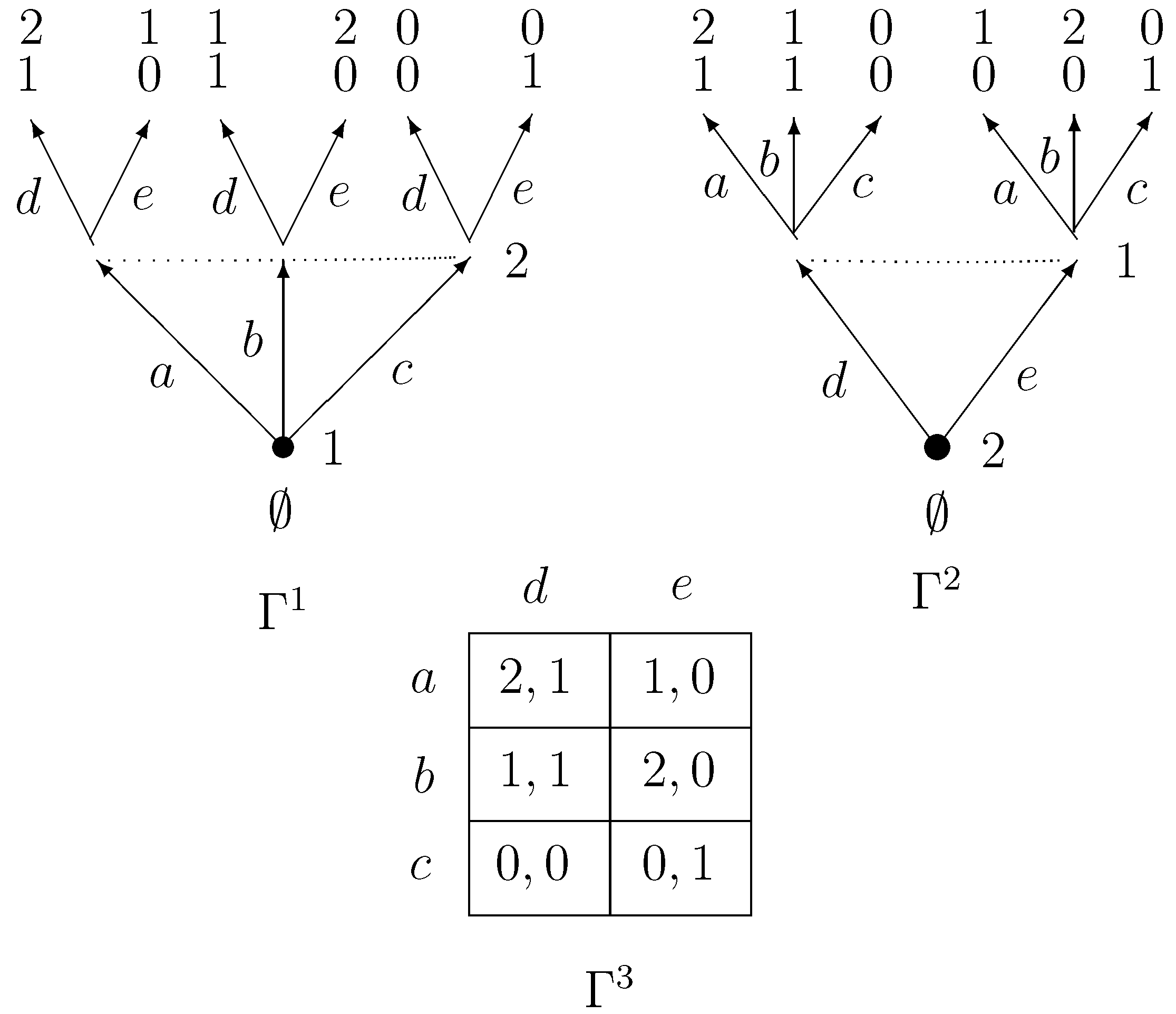
For the concept of common belief in future rationality, it is crucial how we model the chronological order of moves in the game! Consider, for instance, the three games in Figure 2.

Figure 2. Chronological order of moves matters for “common belief in future rationality”.

Figure 2. Chronological order of moves matters for “common belief in future rationality”.

In game ${\Gamma }^1$ player 1 moves before player 2, in game ${\Gamma }^2$ player 2 moves before player 1, and in game ${\Gamma }^3$ both players choose simultaneously. In ${\Gamma }^1$ and ${\Gamma }^2,$ the second mover does not know which choice has been made by the first mover. So, all three games represent a situation in which both players choose in complete ignorance of the opponent’s choice. Since the utilities in the games are identical, one can argue that these three games are in some sense “equivalent”. In fact, the three games above only differ by applying the transformation of interchange of decision nodes2, as defined by Thompson [26]. However, for the concept of common belief in future rationality it crucially matters which of the three representations ${\Gamma }^1,{\Gamma }^2$ or ${\Gamma }^3$ we choose.

In the game ${\Gamma }^1,$ common belief in future rationality does not restrict player 2’s belief at all, as player 1 moves before him. So, player 2 can rationally choose d and e under common belief in future rationality here. On the other hand, player 1 may believe that player 2 chooses d or e under common belief in future rationality, and hence player 1 himself may rationally choose a or b under common belief in future rationality.

In the game ${\Gamma }^2,$ common belief in future rationality does not restrict player 1’s beliefs as he moves after player 2. Hence, player 1 may rationally choose a or b under common belief in future rationality. Player 2 must therefore believe that player 1 will either choose a or b in the future, and hence player 2 can only rationally choose d under common belief in future rationality.

In the game ${\Gamma }^3,$ finally, player 1 can only rationally choose $a,$ and player 2 can only rationally choose d under common belief in future rationality. Namely, if player 2 believes in player 1’s (present and) future rationality, then player 2 believes that player 1 does not choose $c,$ since player 1 moves at the same time as player 2. Therefore, player 2 can only rationally choose d under common belief in future rationality. If player 1 believes in player 2’s (present and) future rationality, and believes that player 2 believes in player 1’s (present and) future rationality, then player 1 believes that player 2 chooses $d,$ and therefore player 1 can only rationally choose a under common belief in future rationality.

Hence, the precise order of moves is very important for the concept of common belief in future rationality! In particular, this concept is not invariant with respect to Thompson’s [26] transformation of interchange of decision nodes. We will come back to this issue in Section 5.3.

3.2. Algorithm

Perea [1] presents an algorithm, backward dominance, that selects exactly those strategies than can rationally be chosen under common belief in future rationality. The algorithm proceeds by successively eliminating, at every information set, some strategies for the players. In the first round we eliminate, at every information set, those strategies for player i that are strictly dominated at a present or future information set for player $i.$ In every further round k we eliminate, at every information set, those strategies for player i that are strictly dominated at a present or future information set h for player $i,$ given the opponents’ strategies that have survived until round k at that information set $h.$ We continue until we cannot eliminate anything more.

In order to formally state the backward dominance procedure, we need the following definitions. Consider an information set $h\in H_i$ for player $i,$ a subset $D_i\subseteq S_i\left(h\right)$ of strategies for player i that possibly reach $h,$ and a subset $D_{-i}\subseteq S_{-i}\left(h\right)$ of strategy combinations for i’s opponents possibly reaching $h.$ Then, $(D_i,D_{-i})$ is called a decision problem for player i at $h,$ and we say that player i is active at this decision problem. Note that several players may be active at the same decision problem, since several players may make a simultaneous move at the associated information set. Within a decision problem $(D_i,D_{-i})$ for player i, a strategy $s_i\in D_i$ is called strictly dominated if there is some randomized strategy ${\mu }_i\in \Delta \left(D_i\right)$ such that $u_i({\mu }_i,s_{-i})>u_i(s_i,s_{-i})$ for all $s_{-i}\in D_{-i}.$ A decision problem at h is said to weakly follow an information set $h^{\prime }$ if h weakly follows $h^{\prime }.$ For a given information set $h\in H_i,$ the full decision problem at h is the decision problem $(S_i\left(h\right),S_{-i}\left(h\right))$ where no strategies have been eliminated yet.

Backward dominance procedure

Initial step. For every information set $h,$ let ${\Gamma }^0\left(h\right)$ be the full decision problem at $h.$

Inductive step. Let $k\ge 1,$ and suppose that the decision problems ${\Gamma }^{k-1}\left(h\right)$ have been defined for every information set $h.$ Then, at every information set h delete from the decision problem ${\Gamma }^{k-1}\left(h\right)$ those strategy combinations that involve a strategy $s_i$ of some player i that is strictly dominated within some decision problem ${\Gamma }^{k-1}\left(h^{\prime }\right)$ for player i that weakly follows $h.$ This yields the new decision problems ${\Gamma }^k\left(h\right).$ Continue this procedure until no further strategies can be eliminated in this way.

Say that a strategy $s_i$ survives the backward dominance procedure if $s_i$ is in ${\Gamma }^k\left(\varnothing \right)$ for every $k.$ That is, $s_i$ is never eliminated in the decision problem at the beginning of the game, $\varnothing .$ Since we only have finitely many strategies in the game, and the decision problems can only become smaller at every step, this procedure must converge after finitely many steps. Perea [1] has shown that the algorithm always yields a nonempty set of strategies at every information set, and that the set of strategies surviving the algorithm is exactly the set of strategies that can rationally be chosen under common belief in future rationality. Combining these two insights then guarantees that common belief in future rationality is always possible—for every player we can always construct a type that expresses common belief in future rationality.

Note than the backward dominance procedure can be alternatively formulated as follows: If at a given decision problem ${\Gamma }^{k-1}\left(h\right)$ for player i strategy $s_i$ is strictly dominated, then we eliminate $s_i$ at ${\Gamma }^{k-1}\left(h\right)$ and at all decision problems ${\Gamma }^{k-1}\left(h^{\prime }\right)$ that come before h—that is, we eliminate $s_i$ from h backwards. So, we can say that the backward dominance procedure, which characterizes the backward induction concept of common belief in future rationality, works by backward elimination. This, in turn, very clearly explains the word backward in backward induction concept.

3.3. Example

We will now illustrate the backward dominance procedure by means of an example. Consider again the game in Figure 1. At the beginning of the procedure we start with two decision problems, namely the full decision problem ${\Gamma }^0\left(\varnothing \right)$ at ∅ where only player 1 is active, and the full decision problem ${\Gamma }^0\left(h_1\right)$ at $h_1$ where both players are active. These decision problems can be found in Table 1.

Table 1. The full decision problems in Figure 1.

Table 1. The full decision problems in Figure 1.

The backward dominance procedure does the following: In the first round, we eliminate from ${\Gamma }^0\left(\varnothing \right)$ strategy $(a,c)$ as it is strictly dominated by b at player 1’s decision problem ${\Gamma }^0\left(\varnothing \right),$ and we eliminate from ${\Gamma }^0\left(\varnothing \right)$ and ${\Gamma }^0\left(h_1\right)$ strategy g as it is strictly dominated by e and f at player 2’s decision problem ${\Gamma }^0\left(h_1\right).$ In the second round, we eliminate from ${\Gamma }^1\left(\varnothing \right)$ strategy $(a,d)$ as it strictly dominated by b at ${\Gamma }^1\left(\varnothing \right),$ and we eliminate strategy $(a,d)$ also from ${\Gamma }^1\left(h_1\right)$ as it is strictly dominated by $(a,c)$ at ${\Gamma }^1\left(h_1\right).$ In the third round, finally, we eliminate from ${\Gamma }^2\left(\varnothing \right)$ and ${\Gamma }^2\left(h_1\right)$ strategy $f,$ as it is strictly dominated by e in ${\Gamma }^2\left(h_1\right).$ So, only strategies b and e remain at $\varnothing .$ Hence, only strategies b and e can rationally be chosen under common belief in future rationality.

4. Extensive Form Rationalizability

We next turn to extensive form rationalizability (Pearce [2], Battigalli [3], Battigalli and Siniscalchi [4]), which is a typical forward induction concept. The idea is as follows: At every information set the corresponding player first asks whether this information set can be reached if his opponents would all choose rationally, that is, would choose optimally for some vectors of conditional beliefs. If so, then at that information set he must only assign positive probability to rational opponents’ strategies. In that case, he then asks: Can this information set also be reached by opponents’ strategies that are optimal if the opponents believe, whenever possible, that their opponents choose rationally? If so, then at that information set he must only assign positive probability to such opponents’ strategies. And so on. So, in a sense, at every information set the associated player looks for the highest degree of mutual belief in rationality that makes reaching this information set possible, and his beliefs at that information set should reflect this highest degree. We first provide a precise epistemic formulation of this concept, and then present an algorithm, iterated conditional dominance, that supports it. We finally illustrate the algorithm by means of an example.

4.1. Epistemic Formulation

The starting point in extensive form rationalizability is that a player, whenever possible, must believe that his opponents choose rationally. That is, if player i is at information set $h\in H_i,$ he first asks whether h could have been reached by rational opponents’ strategies. If so, then at h he must assign positive probability only to rational opponents’ strategies. We say that player i strongly believes in the opponents’ rationality (Battigalli and Siniscalchi [4]).

In order to formalize this idea within an epistemic model, we must make sure that there are “enough” types in the model. To be more precise, if for a given information set $h\in H_i$ there is a rational strategy $s_j$ for opponent j that possibly reaches $h,$ then there must be a type for player j inside the model for which $s_j$ is optimal. Consider, for instance, the game in Figure 1, and suppose that our epistemic model would contain only one type for player 1, which believes that player 2 will choose $e.$ Then, on the one hand, there is a rational strategy for player 1 that reaches $h_1,$ namely $(a,d).$ But the epistemic model does not contain a type for player 1 for which $(a,d)$ is optimal. So, in this case, we must make sure that the epistemic model contains at least one type for player 1 for which $(a,d)$ is optimal.

To guarantee this, it is enough to have a complete epistemic model. Namely, a complete model contains all possible belief hierarchies, so every potentially optimal strategy can be rationalized by at least one type in this model.

To formally define strong belief in the opponents’ rationality, we need the following piece of notation: For every player $i,$ information set $h\in H_i,$ and subset of opponents’ types ${\tilde{T}}_{-i}\subseteq T_{-i},$ let

$${(S_{-i}\left(h\right)\times {\tilde{T}}_{-i})}^{rat}:=\{{(s_j,t_j)}_{j\ne i}\in S_{-i}\left(h\right)\times {\tilde{T}}_{-i}:s_j\mathit{\text{rational}}\mathit{\text{for}}{t}_j\mathit{\text{for}}\mathit{\text{all}}j\ne i\}$$

Recall that strategy $s_j$ is rational for type $t_j$ if $s_j$ is optimal for $t_j$ at every information set in $H_j\left(s_j\right).$

(Strong belief in the opponents’ rationality) Consider a complete epistemic model $M={(T_i,b_i)}_{i\in I}.$ A type $t_i$ strongly believes in the opponents’ rationality if at every $h\in H_i$ with ${(S_{-i}\left(h\right)\times T_{-i})}^{rat}\ne \varnothing ,$ it holds that $b_i(t_i,h)\left({(S_{-i}\left(h\right)\times T_{-i})}^{rat}\right)=1.$

That is, if for every opponent j there is strategy $s_j$ leading to h and a type for which $s_j$ is rational, then type $t_i$ must at h only consider strategy-type pairs $(s_j,t_j)$ where $s_j$ is rational for type $t_j.$ Let us define by $T_i^1$ the set of types $t_i\in T_i$ that strongly believe in the opponents’ rationality.

Now, suppose that player i is at $h\in H_i,$ and that ${(S_{-i}\left(h\right)\times T_{-i})}^{rat}\ne \varnothing .$ So, h could have been reached by rational opponents’ strategies. The next question that extensive form rationalizability asks is: Could h have been reached by opponents’ strategies $s_j$ that are optimal for opponents’ types $t_j$ that strongly believe in their opponents’ rationality? If so, then player i at h should only consider such pairs $(s_j,t_j).$ In other words, if ${(S_{-i}\left(h\right)\times T_{-i}^1)}^{rat}\ne \varnothing ,$ then player i must at h only consider opponents’ strategy-type combinations in ${(S_{-i}\left(h\right)\times T_{-i}^1)}^{rat}.$ By iterating this argument, we arrive at the following recursive definition of common strong belief in rationality (Battigalli and Siniscalchi [4]).

(Common strong belief in rationality) Consider a complete epistemic model $M={(T_i,b_i)}_{i\in I}.$ Let $T_i^0:=T_i$ for every player $i.$ For every $k\ge 1$ and every player $i,$ let $T_i^k$ contain those types $t_i\in T_i^{k-1}$ such that at every $h\in H_i$ with ${(S_{-i}\left(h\right)\times T_{-i}^{k-1})}^{rat}\ne \varnothing ,$ it holds that $b_i(t_i,h)({(S_{-i}\left(h\right)\times T_{-i}^{k-1})}^{rat})=1.$ A type $t_i$ expresses common strong belief in rationality if $t_i\in T_i^k$ for all $k.$

We say that strategy $s_i$ can rationally be chosen under common strong belief in rationality if there is some complete epistemic model $M={(T_i,b_i)}_{i\in I},$ and some type $t_i\in T_i$ expressing common strong belief in rationality, such that $s_i$ is rational for $t_i.$

4.2. Algorithm

The concept of extensive form rationalizability has originally been proposed in Pearce [2] by means of an iterated reduction procedure. Later, Battigalli [3] has simplified this procedure and has shown that it delivers the same output as Pearce’s procedure. Both procedures refine at every round the sets of strategies and conditional beliefs of the players. Battigalli and Siniscalchi [4] have shown that common strong belief in rationality selects exactly the extensive form rationalizable strategies for every player.

In this section we will consider yet another procedure leading to extensive form rationalizability, namely the iterated conditional dominance procedure developed by Shimoji and Watson [22]. The reason is that this procedure is closer to the backward dominance algorithm for common belief in future rationality, and therefore easier to compare.

The iterated conditional dominance procedure, like the backward dominance procedure, iteratedly removes strategies from decision problems. However, the criteria for removing a strategy in a particular decision problem are different. Remember that in the backward dominance procedure we remove a strategy for player i in the decision problem at h whenever it is strictly dominated in some decision problem for player i that weakly follows h. In the iterated conditional dominance procedure we remove a strategy for player i at the decision problem at h if there is some decision problem for player $i,$ not necessarily weakly following $h,$ at which it is strictly dominated. So, in the iterated conditional dominance procedure we would remove strategy $s_i$ at h also if it is strictly dominated at some decision problem for player i that comes before $h.$ Formally, the procedure can be formulated as follows.

Iterated conditional dominance procedure

Initial step. For every information set $h,$ let ${\Gamma }^0\left(h\right)$ be the full decision problem at $h.$

Inductive step. Let $k\ge 1,$ and suppose that the decision problems ${\Gamma }^{k-1}\left(h\right)$ have been defined for every information set $h.$ Then, at every information set h delete from the decision problem ${\Gamma }^{k-1}\left(h\right)$ those strategy combinations that involve a strategy $s_i$ for some player i that is strictly dominated within some decision problem ${\Gamma }^{k-1}\left(h^{\prime }\right)$ for player $i,$ not necessarily weakly following $h.$ This yields the new decision problems ${\Gamma }^k\left(h\right).$ Continue this procedure until no further strategies can be eliminated in this way.

A strategy $s_i$ is said to survive this procedure if $s_i\in {\Gamma }^k\left(\varnothing \right)$ for all $k.$ Shimoji and Watson [22] have shown that this procedure delivers exactly the set of extensive form rationalizable strategies. Hence, by Battigalli and Siniscalchi’s [4] result, the iterated conditional dominance procedure selects exactly those strategies that can rationally be chosen under common strong belief in rationality.

Note that in the iterated conditional dominance procedure, it is possible that at a given decision problem ${\Gamma }^{k-1}\left(h\right)$ all strategies of a player i will be eliminated in step k—something that can never happen in the backward dominance procedure. Consider, namely, some information set $h\in H_i,$ and some information set $h^{\prime }$ following $h.$ Then, it is possible that within the decision problem ${\Gamma }^{k-1}\left(h\right),$ all strategies for player i in ${\Gamma }^{k-1}\left(h^{\prime }\right)$ are strictly dominated. In that case, we would eliminate in ${\Gamma }^{k-1}\left(h^{\prime }\right)$ all remaining strategies for player i! Whenever this occurs, it is understood that at every further step nothing can be eliminated from the decision problem at $h^{\prime }$ anymore.

The iterated conditional dominance procedure thus has the following property: If at a given decision problem ${\Gamma }^{k-1}\left(h\right)$ for player i the strategy $s_i$ is strictly dominated, then we eliminate $s_i$ at ${\Gamma }^{k-1}\left(h\right),$ and at all decision problems ${\Gamma }^{k-1}\left(h^{\prime }\right)$ that come before and after it—that is, we eliminate $s_i$ from h backwards and forward. So this algorithm, which characterizes the forward induction concept of extensive form rationalizability, proceeds by backward and forward elimination. From this perspective, the name “forward induction” is actually a bit misleading, as it would suggest the concept to work only in a forward fashion. This is not true: Extensive form rationalizability, when considered algorithmically, works both backwards and forward.

4.3. Example

To illustrate the iterated conditional dominance procedure, consider again the game from Figure 1, with its full decision problems ${\Gamma }^0\left(\varnothing \right)$ and ${\Gamma }^0\left(h_1\right)$ as depicted in Table 1. The iterated conditional dominance procedure works as follows here:

In the first round, we eliminate strategy $(a,c)$ from ${\Gamma }^0\left(\varnothing \right)$ and ${\Gamma }^0\left(h_1\right)$ as it is strictly dominated by b at player 1’s decision problem ${\Gamma }^0\left(\varnothing \right),$ and we eliminate from ${\Gamma }^0\left(\varnothing \right)$ and ${\Gamma }^0\left(h_1\right)$ strategy g as it is strictly dominated by e and f at player 2’s decision problem ${\Gamma }^0\left(h_1\right).$ In the second round, we eliminate $(a,d)$ from ${\Gamma }^1\left(\varnothing \right)$ and ${\Gamma }^1\left(h_1\right)$ as it is strictly dominated by b at ${\Gamma }^1\left(\varnothing \right),$ and we eliminate e from ${\Gamma }^1\left(\varnothing \right)$ and ${\Gamma }^1\left(h_1\right)$ as it is strictly dominated by f in ${\Gamma }^1\left(h_1\right).$ This only leaves strategies b and f at $\varnothing ,$ and hence only strategies b and f can rationally be chosen under extensive form rationalizability.

Recall that the backward dominance procedure uniquely selected strategies b and $e,$ and hence only e can rationally be chosen by player 2 under common belief in future rationality. So, we see that both procedures (and hence their associated epistemic concepts) lead to unique but different strategy choices for player 2 in this example.

The crucial difference between both concepts lies in how player 2 at $h_1$ explains the surprise that player 1 has not chosen $b.$ Under common belief in future rationality, player 2 believes at $h_1$ that player 1 has simply made a mistake, but he still believes that player 1 will choose rationally at $h_1,$ and he still believes that player 1 believes that he will not choose g at $h_1.$ So, player 2 believes at $h_1$ that player 1 will choose $(a,c),$ and therefore player 2 will choose e at $h_1.$ Under extensive form rationalizability, player 2 believes at $h_1$ that player 1’s decision not to choose b was a rational decision, but this is only possible if player 2 believes at $h_1$ that player 1 believes that player 2 will irrationally choose g at $h_1$ (with sufficiently high probability). In that case, player 2 will believe at $h_1$ that player 1 will go for $(a,d),$ and therefore player 2 will choose f at $h_1.$

5. Comparision Between the Concepts

In this section we will compare the concepts of common belief in future rationality and extensive form rationalizability (common strong belief in rationality) on a conceptual, epistemic, algorithmic and behavioral level.

5.1. Conceptual Comparison: The Role of Rationality Orderings

An appealing way to look at extensive form rationalizability is by means of rationality orderings over strategies (Battigalli [29]). The idea is that for every player i we have an ordered partition $(S_i^1,...,S_i^K)$ of his strategy set, where $S_i^1$ represents the set of “most rational” strategies, $S_i^K$ the set of “least rational” strategies, and every strategy in $S_i^k$ is deemed “more rational” than every strategy in $S_i^{k+1}.$ At every information set $h\in H_i,$ player i then looks for the most rational opponents’ strategies that reach $h,$ and assigns positive probability only to such opponents’ strategies. Important is that these rationality ordering are global, that is, the players always use the same rationality orderings over the opponents’ strategies to form their conditional beliefs.

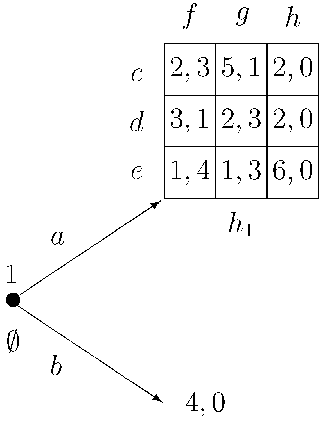
To illustrate this, consider the game in Figure 3.

Figure 3. Rationality orderings.

Figure 3. Rationality orderings.

Among player 1’s strategies, $(a,c),(a,e)$ and b are optimal for some belief, whereas $(a,d)$ is not optimal for any belief. So, $(a,d)$ may be considered the “least rational” strategy for player 1. So, for player 1 we have the “tentative” rationality ordering

$$R{O}_1^1=(\{(a,c),(a,e),b\},\left\{(a,d)\right\})$$

For player 2, strategies f and g are optimal at $h_1$ for some belief, whereas h is not optimal at $h_1$ for any belief. Hence, for player 2 we have the tentative rationality ordering

$$R{O}_2^1=(\{f,g\},\left\{h\right\})$$

Now, if player 1 believes that player 2 does not choose his least rational strategy $h,$ then only $(a,c)$ and b can be optimal, and not $(a,e)$. So, we obtain a refined rationality ordering

$$R{O}_1^2=(\{(a,c),b\},\left\{(a,e)\right\},\left\{(a,d)\right\})$$

for player 1. Similarly, if player 2 believes at $h_1$ that player 1 will not choose his least rational strategy $(a,d),$ then only f can be optimal, and not $g.$ So, for player 2 we obtain the refined rationality ordering

$$R{O}_2^2=(\left\{f\right\},\left\{g\right\},\left\{h\right\})$$

But then, if player 1 believes that player 2 will choose his most rational strategy $f,$ then player 1 will choose $b.$ So, the final rationality orderings for the players are

$$R{O}_1=(\left\{b\right\},\left\{(a,c)\right\},\left\{(a,e)\right\},\left\{(a,d)\right\})\mathit{\text{and}}R{O}_2=(\left\{f\right\},\left\{g\right\},\left\{h\right\})$$

Hence, if player 2 finds himself at $h_1,$ he believes that player 1 has chosen the most rational strategy that reaches $h_1,$ which is $(a,c).$ Player 2 must therefore choose $f,$ and player 1, anticipating on this, should choose $b.$ This is exactly what extensive form rationalizability does for this game.

Important is that both players agree on these specific rationality orderings $R{O}_1$ and $R{O}_2,$ and that player 2 uses the rationality ordering $R{O}_1$ throughout the game, in particular at $h_1$ to form his conditional belief there.

In contrast, the concept of common belief in future rationality cannot be described in terms of rationality orderings, or at least not by global rationality orderings that are used throughout the whole game. Consider again the game in Figure 3. Common belief in future rationality reasons as follows here: Player 1, at ∅ and at $h_1,$ must believe that player 2 chooses rationally at $h_1,$ and hence must believe that player 2 will not choose $h.$ Player 2, at $h_1,$ believes that player 1, at $h_1,$ believes in 2’s rationality at $h_1.$ Hence, player 2 believes at $h_1$ that player 1 believes that 2 will not choose $h.$ Also, player 2 believes at $h_1$ that player 1 chooses rationally at $h_1,$ and hence player 2 believes at $h_1$ that player 1 will not choose $(a,e)$. No further conclusions can be drawn at $h_1.$ Hence, player 2 can choose f or g at $h_1.$ But then, player 1 can choose $(a,c)$ or $b.$ So, common belief in future rationality selects strategies $(a,c)$ and b for player 1, and strategies f and g for player 2.

Can this reasoning be represented by global rationality orderings on the players’ strategies? The answer is “no”. Suppose, namely, that such rationality orderings $R{O}_1$ and $R{O}_2$ would exist. As common belief in future rationality selects only the strategies $(a,c)$ and b for player 1, strategies $(a,c)$ and b should both be most rational under $R{O}_1.$ But then, if player 2 is at $h_1,$ he should conclude that player 1 has chosen $(a,c),$ as it is the most rational strategy under $R{O}_1$ that reaches $h_1.$ Consequently, player 2 should choose $f,$ rendering $(a,c)$ a suboptimal strategy for player 1. This, however, would contradict $R{O}_1,$ where $(a,c)$ is considered to be a most rational strategy for player 1. Hence, there is no global rationality ordering on strategies that supports common belief in future rationality.

Rather, under common belief in future rationality, player 2 changes his rationality ordering over 1’s strategies as the game proceeds. At the beginning, player 2 deems $(a,c)$ and b more rational then $(a,d)$ and $(a,e).$ However, at $h_1$ player 2 deems $(a,c)$ and $(a,d)$ “equally” rational, as under common belief in future rationality player 2 may at $h_1$ believe that player 1 chooses $(a,c)$ or $(a,d).$

5.2. Epistemic Comparison

By definition, a type $t_i$ for player i is said to express common belief in future rationality if it always believes in the opponents’ future rationality, always only assigns positive probability to opponents’ types that always believe in their opponents’ future rationality, always only assigns positive probability to opponents’ types that always only assign positive probability to other players’ types that always believe in their opponents’ future rationality, and so on. As a consequence, type $t_i$ always only assigns positive probability to opponents’ types that express common belief in future rationality too. Hence, every type that expresses common belief in future rationality believes at every stage of the game that each of his opponents expresses common belief in future rationality as well. We may thus say that the concept of common belief in future rationality is “closed under belief”.

Formally, “closed under belief” can be defined in the following way. Consider some epistemic model with sets of types $T_i$ for every player i. Let ${\widehat{T}}_i\subseteq T_i$ be a subset of types for every player $i.$ Then, the combination ${({\widehat{T}}_i)}_{i\in I}$ of subsets of types is said to be closed under belief if for every player $i,$ every type $t_i\in {\widehat{T}}_i,$ and every information set $h\in H_i,$ the conditional belief $b_i({\widehat{t}}_i,h)$ only assigns positive probability to opponents’ types $t_j$ that are in ${\widehat{T}}_j.$ So if we take an epistemic model with sets of types ${\left(T_i\right)}_{i\in I},$ and define $T_i^{cbfr}\subseteq T_i$ to be the subset of types for player i that express common belief in future rationality, then the combination ${(T_i^{cbfr})}_{i\in I}$ of type subsets expressing common belief in future rationality is closed under belief in the sense above.

The same cannot be said about common strong belief in rationality—the epistemic foundation for extensive form rationalizability. Consider for instance the game from Figure 1. If player 2’s type $t_2$ strongly believes in player 1’s rationality, then $t_2$ must at $h_1$ believe that player 1 has rationally chosen $(a,d).$ More precisely, type $t_2$ must at $h_1$ only assign positive probability to strategy-type pairs $((a,d),t_1)$ for player 1 where $(a,d)$ is optimal for type $t_1.$ This, however, can only be the case if $t_1$ assigns positive probability to player 2’s irrational strategy $g.$ But then, $t_1$ does certainly not strongly believe in 2’s rationality. So we see that a type $t_2$ for player 2 who strongly believes in 1’s rationality, must at $h_1$ necessarily assign positive probability to a type $t_1$ for player 1 who does not strongly believe in 2’s rationality. In particular, a type $t_2$ for player 2 that expresses common strong belief in rationality, must at $h_1$ attach positive probability to a player 1 type $t_1$ that does not express common strong belief in rationality. Hence, the concept of common strong belief in rationality is certainly not closed under belief.

The latter is not surprising, as it follows from the very character of common strong belief in rationality. As we have seen in the previous subsection, this concept orders the players’ strategies, and also types, from “most rational” to “least rational”. Most rational are the types that express common strong belief in rationality, and least rational are the types that do not even strongly believe in the opponents’ rationality, and there may be some subclasses in between. The idea of common strong belief in rationality is that at every information set, the corresponding player searches for the “most rational” opponents’ types that could have been responsible for reaching this information set, and these opponents’ types do not necessarily express common strong belief in rationality. In fact, typically these opponents’ types are “less rational” than the “most rational types around”, which are the ones expressing common strong belief in rationality. So, it is no surprise that the concept of common strong belief in rationality is not “closed under belief”.

The fact that common belief in future rationality is closed under belief, and common strong belief in rationality is not, is also reflected in the completeness of the epistemic model needed for these two concepts. Note that for defining common strong belief in rationality we required a complete epistemic model (meaning that every possible belief hierarchy is present in the model), whereas for common belief in future rationality we did not. In fact, for the concept of common belief in future rationality a model with finitely many types is enough (see Perea [1]). So why do we have this difference?

The reason is that under common strong belief in rationality, player i must ask at every information set $h\in H_i$ whether h could have been reached by opponents’ strategies that are optimal for some beliefs. To answer this question, he must consider all possible opponents’ types—also those that do not express common strong belief in rationality—and see whether some of these types would support strategy choices that could lead to $h.$ So, a complete epistemic model is needed here.

In contrast, under common belief in future rationality it is sufficient for player i to only consider opponents’ types that express common belief in future rationality as well. In other words, there is no need for player i to step outside the sets of types expressing common belief in future rationality, and that is why we do not need a complete epistemic model here.

5.3. Algorithmic Comparison

In Section 3 and Section 4 we have described two elimination procedures, backward dominance and iterated conditional dominance, that respectively lead to common belief in future rationality and extensive form rationalizability. A natural question is: Does the order and speed in which we eliminate strategies from the decision problems matter for the eventual result of these procedures? The answer is that it does not matter for the backward dominance procedure (see Perea [1]), whereas the order and speed of elimination is crucial for the iterated conditional dominance procedure.

Consider, namely, the game from Figure 1. Suppose that, in the first round of the iterated conditional dominance procedure, we would only eliminate strategy $g,$ but not $(a,c),$ from ${\Gamma }^0\left(\varnothing \right)$ and ${\Gamma }^0\left(h_1\right).$ Then, in ${\Gamma }^1\left(h_1\right),$ strategy $(a,d)$ is strictly dominated by $(a,c).$ Suppose that in round 2 we would only eliminate strategy $(a,d)$ from ${\Gamma }^1\left(\varnothing \right)$ and ${\Gamma }^1\left(h_1\right).$ Suppose that in round 3 we would eliminate strategy f for player 2 at ∅ and $h_1,$ as it has become strictly dominated at $h_1.$ Suppose that, finally, we would eliminate $(a,c)$ at ∅ and $h_1.$ So, for player 2 only strategy e would survive the procedure in this case. Recall, however, that if we eliminate “all that we can” at every round of the iterated conditional dominance procedure, then only strategy f would survive for player 2. Hence, the order and speed of elimination affects the outcome of the iterated conditional dominance procedure—it is absolutely crucial to eliminate at every round, and at every information set, all strategies we can.

Now, why is the order and speed of elimination relevant for the iterated conditional dominance procedure, but not for the backward dominance procedure? The reason has to do with rationality orderings as we have discussed them above. We have seen that extensive form rationalizability can be described by global rationality orderings on the players’ strategies, ranking them from “most rational” to “least rational”. At every information set, the corresponding player identifies the most rational opponents’ strategies that reach this information set, and assigns positive probability only to these strategies. For this construction to work, it is essential that all players agree on these specific rationality orderings.

The iterated conditional dominance procedure in fact generates these rationality orderings: All strategies that do not survive the first round are deemed “least rational”. All strategies that survive the first round, but not the second round, are deemed “second least rational” and so on. Finally, the strategies that survive all rounds are deemed “most rational”. So, this procedure does not only deliver the extensive form rationalizable strategies, it also delivers the rationality orderings on players’ strategies that support extensive form rationalizability. Since it is crucial that players agree on these rationality orderings, players must agree on the strategies that are eliminated at every round of the procedure: If at a certain round not all strategies that could be eliminated are in fact eliminated, then this would lead to a “coarser” rationality ordering in that round, which in turn could lead to completely different rationality orderings in the end.

This problem cannot occur for backward dominance: If at a certain information set a strategy that could have been eliminated is not in fact eliminated, then it will be eliminated at some later round anyhow. So, even if players would disagree on the order and speed of elimination, it would not affect their final strategy choices in the game.

We have seen in Section 3 that the concept of common belief in future rationality is sensitive to the transformation of interchange of decision nodes, as defined by Thompson [26]. This can be seen very clearly from its associated algorithm—the backward dominance procedure. In this algorithm, namely, whenever a strategy $s_i$ is strictly dominated at a decision problem ${\Gamma }^{k-1}\left(h\right)$ for player $i,$ we eliminate it from ${\Gamma }^{k-1}\left(h\right)$ and all decision problems ${\Gamma }^{k-1}\left(h^{\prime }\right)$ that come before h, but we do not eliminate it at decision problems ${\Gamma }^{k-1}\left(h^{\prime }\right)$ that come after $h.$ By applying the transformation of interchange of decision nodes, we may interchange the chronological order of two information sets h and $h^{\prime }.$ So, before the transformation h comes before $h^{\prime },$ whereas after the transformation $h^{\prime }$ comes before $h.$ Hence it is possible that before the transformation we eliminate $s_i$ at h because it is strictly dominated at $h^{\prime },$ whereas after the transformation we can no longer do so because h now comes after $h^{\prime }.$ That is, the transformation of interchange of decision nodes may have important consequences for the output of the backward dominance procedure—and hence for the concept of common belief in future rationality.

It can be verified that the transformation of interchange of decision nodes has no consequences for the concept of extensive form rationalizability. This is most easily seen by studying the associated algorithm—the iterated conditional dominance procedure. In that procedure, whenever a strategy $s_i$ is strictly dominated at a decision problem ${\Gamma }^{k-1}\left(h\right)$ for player $i,$ we eliminate it at all decision problems ${\Gamma }^{k-1}\left(h^{\prime }\right)$ in the game. Hence, the precise chronological order of the information sets does not play a role, only the structure of the various decision problems ${\Gamma }^{k-1}\left(h\right)$ in the game. Since the transformation of interchange of decision nodes does not change this structure of the decision problems ${\Gamma }^{k-1}\left(h\right)$ in the game, it easily follows that the iterated conditional dominance procedure—and hence the concept of extensive form rationalizability—is invariant under the transformation of interchange of decision nodes.

5.4. Behavioral Comparison

In this section we ask whether there is any logical relationship between the strategy choices selected by common belief in future rationality, and those selected by extensive form rationalizability. The answer is “no”. This can already be concluded from the example in Figure 1. There, we have seen that common belief in future rationality uniquely selects strategy e for player 2, whereas extensive form rationalizability uniquely selects strategy f for this player. Hence, in this example both concepts yield completely opposite strategy selections for player 2.

There are other examples where common belief in future rationality is more restrictive than extensive form rationalizability, and yet other examples where it is exactly the other way around. Consider, for instance, the game from Figure 3. There, common belief in future rationality yields strategy choices $(a,c)$ and b for player 1, and strategy choices f and g for player 2. Extensive form rationalizability, on the other hand, uniquely selects strategies b and $f.$ So here extensive form rationalizability is more restrictive.

Now, replace in the example in Figure 1 the outcome $3,0$ by $5,0.$ Then, common belief in future rationality would select strategy b for player 1, and strategy e for player 2, whereas extensive form rationalizability would select strategy b for player 1, and strategies e and f for player 2. So here common belief in future rationality is more restrictive.

Note, however, that in each of these examples the set of outcomes induced by extensive form rationalizability is always a subset of the set of outcomes induced by common belief in future rationality. My conjecture is that this is true in general, but I could not find a formal proof yet. (In fact we know that it is true for all generic games with perfect information – see the paragraph below). So I leave this here as an interesting open problem.

An important special class of dynamic games, both for theory and applications, is the class of games with perfect information. These are games where at every stage only one player moves, and he always observes the choices made by others so far. Such a game is called generic if, for every player i and every information set $h\in H_i,$ two different choices at h always lead to outcomes with different utilities for $i.$

In Perea [1] it has been shown that for the class of generic dynamic games with perfect information, the concept of common belief in future rationality leads to the unique backward induction strategies for the players. Battigalli [3] has proved that extensive form rationalizability, and hence common strong belief in rationality, leads to the backward induction outcome, but not necessarily to the backward induction strategies, in such games. As a consequence, for generic games with perfect information both concepts lead to the same outcome, namely the backward induction outcome, but not necessarily to the same strategies for the players.

References

- Perea, A. Belief in the opponents’ future rationality. Maastricht University: Maastricht, The Netherlands, 2010. (manuscript). Available oneline: http://www.personeel.unimaas.nl/a.perea/ (accessed on 1 June 2010).
- Pearce, D.G. Rationalizable strategic behavior and the problem of perfection. Econometrica 1984, 52, 1029–1050. [Google Scholar] [CrossRef]
- Battigalli, P. On rationalizability in extensive games. J. Econ. Theor. 1997, 74, 40–61. [Google Scholar] [CrossRef]
- Battigalli, P.; Siniscalchi, M. Strong belief and forward induction reasoning. J. Econ. Theor. 2002, 106, 356–391. [Google Scholar] [CrossRef]
- Zermelo, E. Über eine Anwendung der Mengenlehre auf die Theorie des Schachspiels. In Proceedings Fifth International Congress of Mathematicians, Cambridge, UK, 22–28 August 1912; pp. 501–504.
- Kreps, D.M.; Wilson, R. Sequential equilibria. Econometrica 1982, 50, 863–94. [Google Scholar] [CrossRef]
- Bernheim, B.D. Rationalizable strategic behavior. Econometrica 1984, 52, 1007–1028. [Google Scholar] [CrossRef]
- Aumann, R.; Brandenburger, A. Epistemic conditions for Nash equilibrium. Econometrica 1995, 63, 1161–1180. [Google Scholar] [CrossRef]
- Asheim, G.B. The Consistent preferences approach to deductive reasoning in games. In Theory and Decision Library; Springer: Dordrecht, The Netherlands, 2006. [Google Scholar]
- Perea, A. A one-person doxastic characterization of Nash strategies. Synthese 2007, 158, 251–271, (Knowledge, Rationality & Action, 341–361). [Google Scholar] [CrossRef]
- Dekel, E.; Fudenberg, D.; Levine, D.K. Payoff information and self-confirming equilibrium. J. Econ. Theor. 1999, 89, 165–185. [Google Scholar] [CrossRef]
- Dekel, E.; Fudenberg, D.; Levine, D.K. Subjective uncertainty over behavior strategies: A correction. J. Econ. Theor. 2002, 104, 473–478. [Google Scholar] [CrossRef]
- Asheim, G.B.; Perea, A. Sequential and quasi-perfect rationalizability in extensive games. Game. Econ. Behav. 2005, 53, 15–42. [Google Scholar] [CrossRef]
- Penta, A. Robust dynamic mechanism design. University of Pennsylvania: Philadelphia, PA, USA, 2009; (manuscript). [Google Scholar]
- McLennan, A. Justifiable beliefs in sequential equilibria. Econometrica 1985, 53, 889–904. [Google Scholar] [CrossRef]
- Cho, I.-K. A refinement of sequential equilibrium. Econometrica 1987, 55, 1367–1389. [Google Scholar] [CrossRef]
- Hillas, J. Sequential equilibria and stable sets of beliefs. J. Econ. Theor. 1994, 64, 78–102. [Google Scholar] [CrossRef]
- Cho, I.-K.; Kreps, D.M. Signaling games and stable equilibria. Quart. J. Econ. 1987, 102, 179–221. [Google Scholar] [CrossRef]
- Kohlberg, E.; Mertens, J.-F. On the strategic stability of equilibria. Econometrica 1986, 54, 1003–1038. [Google Scholar] [CrossRef]
- Reny, P.J. Backward induction, normal form perfection and explicable equilibrium. Econometrica 1992, 60, 627–649. [Google Scholar] [CrossRef]
- Govindan, S.; Wilson, R. On forward induction. Econometrica 2009, 77, 1–28. [Google Scholar] [CrossRef]
- Shimoji, M.; Watson, J. Conditional dominance, rationalizability, and game forms. J. Econ. Theor. 1998, 83, 161–195. [Google Scholar] [CrossRef]
- Rubinstein, A. Comments on the interpretation of game theory. Econometrica 1991, 59, 909–924. [Google Scholar] [CrossRef]
- Ben-Porath, E. Rationality, Nash equilibrium and backwards induction in perfect-information games. Rev. Econ. Stud. 1997, 64, 23–46. [Google Scholar] [CrossRef]
- Battigalli, P.; Siniscalchi, M. Hierarchies of conditional beliefs and interactive epistemology in dynamic games. J. Econ. Theor. 1999, 88, 188–230. [Google Scholar] [CrossRef]
- Thompson, F.B. Equivalence of games in extensive form. The Rand Corporation: Santa Monica, CA, USA, 1952; Discussion Paper RM 759. [Google Scholar]
- Elmes, S.; Reny, P.J. On the strategic equivalence of extensive form games. J. Econ. Theor. 1994, 62, 1–23. [Google Scholar] [CrossRef]
- Perea, A. Rationality in Extensive Form Games. In Theory and Decision Library, Series C; Kluwer Academic Publishers: London, UK, 2001. [Google Scholar]
- Battigalli, P. Strategic rationality orderings and the best rationalization principle. Game. Econ. Behav. 1996, 13, 178–200. [Google Scholar] [CrossRef]
- 1.Here, by a rational strategy we mean a strategy that is optimal, at every information set, for some probabilistic belief about the opponents’ strategy choices.
© 2010 by the author; licensee MDPI, Basel, Switzerland. This article is an open access article distributed under the terms and conditions of the Creative Commons Attribution license http://creativecommons.org/licenses/by/3.0/.
Share and Cite
MDPI and ACS Style
Perea, A. Backward Induction versus Forward Induction Reasoning. Games 2010, 1, 168-188. https://0-doi-org.brum.beds.ac.uk/10.3390/g1030168
AMA Style
Perea A. Backward Induction versus Forward Induction Reasoning. Games. 2010; 1(3):168-188. https://0-doi-org.brum.beds.ac.uk/10.3390/g1030168
Chicago/Turabian StylePerea, Andres. 2010. "Backward Induction versus Forward Induction Reasoning" Games 1, no. 3: 168-188. https://0-doi-org.brum.beds.ac.uk/10.3390/g1030168