Game-Theoretic Optimal Portfolios for Jump Diffusions


Department of Economics, Northern Illinois University, 514 Zulauf Hall, DeKalb, IL 60115, USA
Games 2019, 10(1), 8; https://0-doi-org.brum.beds.ac.uk/10.3390/g10010008
Submission received: 17 December 2018
/
Revised: 2 February 2019
/
Accepted: 10 February 2019
/
Published: 13 February 2019
Abstract
:This paper studies a two-person trading game in continuous time that generalizes Garivaltis (2018) to allow for stock prices that both jump and diffuse. Analogous to Bell and Cover (1988) in discrete time, the players start by choosing fair randomizations of the initial dollar, by exchanging it for a random wealth whose mean is at most 1. Each player then deposits the resulting capital into some continuously rebalanced portfolio that must be adhered to over . We solve the corresponding “investment -game”, namely the zero-sum game with payoff kernel , where is player i’s fair randomization, is the final wealth that accrues to a one dollar deposit into the rebalancing rule b, and is any increasing function meant to measure relative performance. We show that the unique saddle point is for both players to use the (leveraged) Kelly rule for jump diffusions, which is ordinarily defined by maximizing the asymptotic almost-sure continuously compounded capital growth rate. Thus, the Kelly rule for jump diffusions is the correct behavior for practically anybody who wants to outperform other traders (on any time frame) with respect to practically any measure of relative performance.
Keywords:
portfolio choice; continuously rebalanced portfolios; Kelly criterion; log-optimal investment; minimax; jump processesJEL Classification:
C44; D80; D81; G111. Introduction
1.1. Literature Review
Bell and Cover [1] studied a static, zero-sum competitive investment game whose payoff kernel is the probability that Player 1 has more wealth than Player 2 after a single period’s fluctuation of the stock market. They found it necessary to introduce the device of “fair randomization” of the initial dollar for a random capital whose mean is at most 1. This being done, in equilibrium both players use the Kelly [2] rule (or log-optimal portfolio) in conjunction with uniform (0, 2) randomizations of the initial dollar.
Kelly [2] initially found his criterion by considering repeated bets on horse races by a wire fraudster whose advance knowledge is not reliable. Kelly’s example, which is beautiful in its simplicity, leads one to recover the logarithm as the “correct” utility function. As naturally as ever, Kelly considered fixed-fraction betting schemes and found the one with the highest possible almost-sure asymptotic capital growth rate. This gave him his “New Interpretation of the Information Rate” of the wire.
Bell and Cover’s [3] sequel replaces the probability of outperformance by the expectation of some arbitrary measure of the two gamblers’ relative performance. They again found that the Kelly rule reigns supreme, along with fair randomizations that are completely characterized by . Thus, for practically any egotist whose only goal is to outperform other traders over the short term (by whatever his personal criterion), the correct behavior is specified by the Kelly criterion. Well, maybe not correct for everybody: Samuelson’s [4] simplified approach to critiquing the Kelly rule uses only one-syllable words.
Garivaltis [5] wanted to see whether or not Bell and Cover’s results hold up in the context of a stochastic differential investment -game for several Itô processes with state-dependent drift and diffusion. They do; the correct behavior is to use Bell and Cover’s [3] randomizations in conjunction with the feedback control policy , which is the local version of the multivariate Kelly rule in continuous time. Here, is the local drift vector, is the local covariance matrix of instantaneous returns per unit time, and is a vector of ones.
1.2. Contribution
The present paper extends the analysis of Garivaltis [5] to a general stock market where security prices both jump and diffuse, as introduced by Merton [6]. We define the corresponding leveraged Kelly rule and show that it is the unique saddle point of the expected ratio of the players’ final wealths. Jumps arrive at an expected rate of per unit time; when the diffusion parameters are zeroed out, we recover Bell and Cover [3], albeit with the proviso that the players must twiddle their thumbs while waiting for jumps to arrive. In this connection, we have extended Bell and Cover’s analysis to allow for leveraged portfolios in so far as solvency can be guaranteed for all possible jump realizations in some compact, arbitrage-free support . For background material on market games featuring this type of environment (i.e., compactly supported jump returns), we refer the interested reader to the book by Bernhard et al. [7].
2. Investment -Game for Jump Diffusions
We consider a two-person trading game in continuous time that generalizes Garivaltis [5]. A discrete-time version of the game was studied by Bell and Cover [1,3]. The game has several moving parts, which we discuss presently. Each player starts with a dollar.
Definition 1.
By afair randomizationof the initial dollar is a random wealth distributed over such that .
Example 1.
.
Example 2.
, where Z is a unit normal.
Example 3.
with certainty.
At the start of the game, each player picks a fair randomization of his initial dollar. He then deposits the resulting capital into a continuously rebalanced portfolio over a stock market with n correlated securities whose prices both jump and diffuse.
Jumps arrive according to a Poisson process, at an expected rate of jumps per unit time. We let denote the number of jumps that occured over . Thus, we have and
We let denote the price of stock i at time t, where . The gross-returns on jumps are random vectors , where is the gross-return on stock i for a jump that occurs at t. We let be the net return, and we write for the vector of net returns on a jump. We assume that jumps are drawn iid according to some CDF .
The general law of motion for the price of stock i is given by
where and are the drift and volatility, respectively, of stock i, and is a standard Brownian motion. We let be the correlation of the unanticipated (diffusive) instantaneous returns of stocks i and j. We let denote the covariance of instantaneous returns per unit time. We assume that the matrix is invertible, and therefore positive definite. All sources of randomness in the game, namely , and are assumed to be mutually independent.
We allow each player to use a leveraged, continuously rebalanced portfolio (or fixed-fraction betting scheme) that continuously maintains some fixed fraction of wealth in each stock i. Thus, a constant rebalancing rule is a vector . During diffusion, the rebalancing rule b must trade continuously (in small amounts) so as to counteract allocation drift. Immediately after jumps, the gambler must execute comparatively large rebalancing trades so as to restore the target allocation of wealth in each stock i.
We assume that there is a risk-free bond whose price follows . We let denote the wealth at t that accrues to a deposit into the rebalancing rule b. Thus, the trader owns shares of stock i at time t. The remaining dollars are invested in bonds. While diffusing, there is no risk of bankruptcy over the differential time interval , no matter how much leverage is used. However, in order to avoid bankruptcy after jumps , there must be limits on how much leverage each trader can use.
Accordingly, we assume the net return vectors have a closed and bounded support, denoted . Limited liability means that is bounded below by the vector , e.g., . generates a corresponding set of non-bankruptable (admissible) rebalancing rules, where
Here is the gross-return of the rebalancing rule b during a jump. We assume that no bond interest is received (or paid) during a jump, since no time elapses. During diffusion, the trader’s margin loan balance is . Thus, he maintains a constant debt-to-assets ratio of .
Proposition 1.
The action set is nonempty, convex, and open.
Proof.
First, note that . Next, since is an intersection of half spaces, it is convex. Finally, define the function By the Theorem of the Minimum [8], is continuous, since is compact. Note that if and only if . Thus, is open, since it is the preimage of the open set under a continuous mapping. □
We will assume that does not allow arbitrage, in the sense that
Example 4.
The net return support is disallowed, because The gambler could take out an arbitrarily large margin loan and earn an infinite, riskless profit on the first jump that occurs. We have and
Example 5.
For a market with a single stock whose jumps have a net return where , we have
The wealth that accrues to a one dollar deposit into b evolves according to
where is an vector of ones. The trader’s growth factor from jumps is , where is the net return vector of the jump. Applying Itô’s lemma for several diffusions [9], the trader’s growth factor from diffusion is . Thus, we have the formula
Definition 2.
The investment -game is the two-person zero-sum game with payoff kernel
where Player 1 (numerator, maximizing) picks a rebalancing rule and a fair randomization , and Player 2 (denominator, minimizing) picks a rebalancing rule and a fair randomization . is any increasing function meant to measure the relative performance of the two traders. Player 1’s payoff is and Player 2’s payoff is .
Example 6.
. This turns the payoff kernel into the probability that Player 1 has more final wealth than Player 2.
Example 7.
. We get the probability that Player 1 achieves at least the fraction α of the final wealth of Player 2.
Example 8.
, for .
Example 9.
. This turns the payoff kernel into , e.g., the expected ratio of Player 1’s wealth to the aggregate wealth.
3. The Basic Saddle Point
We start by solving the simplified game with payoff kernel . This will culminate in
Theorem 1.
The maximin strategy and the minimax strategy are both equal to the Kelly rule (log-optimal continuously rebalanced portfolio) for jump diffusions.
In preparation for proving the theorem, we explain and define the Kelly rule for jump diffusions. The trader’s realized continuously compounded capital growth rate over is
which converges to as . The asymptotic growth rate is strictly concave over .
Definition 3.
The Kelly rule for jump diffusions is the (unique) rebalancing rule that maximizes the asymptotic continuously-compounded capital growth rate. It is characterized by the first order condition
Next, we calculate that
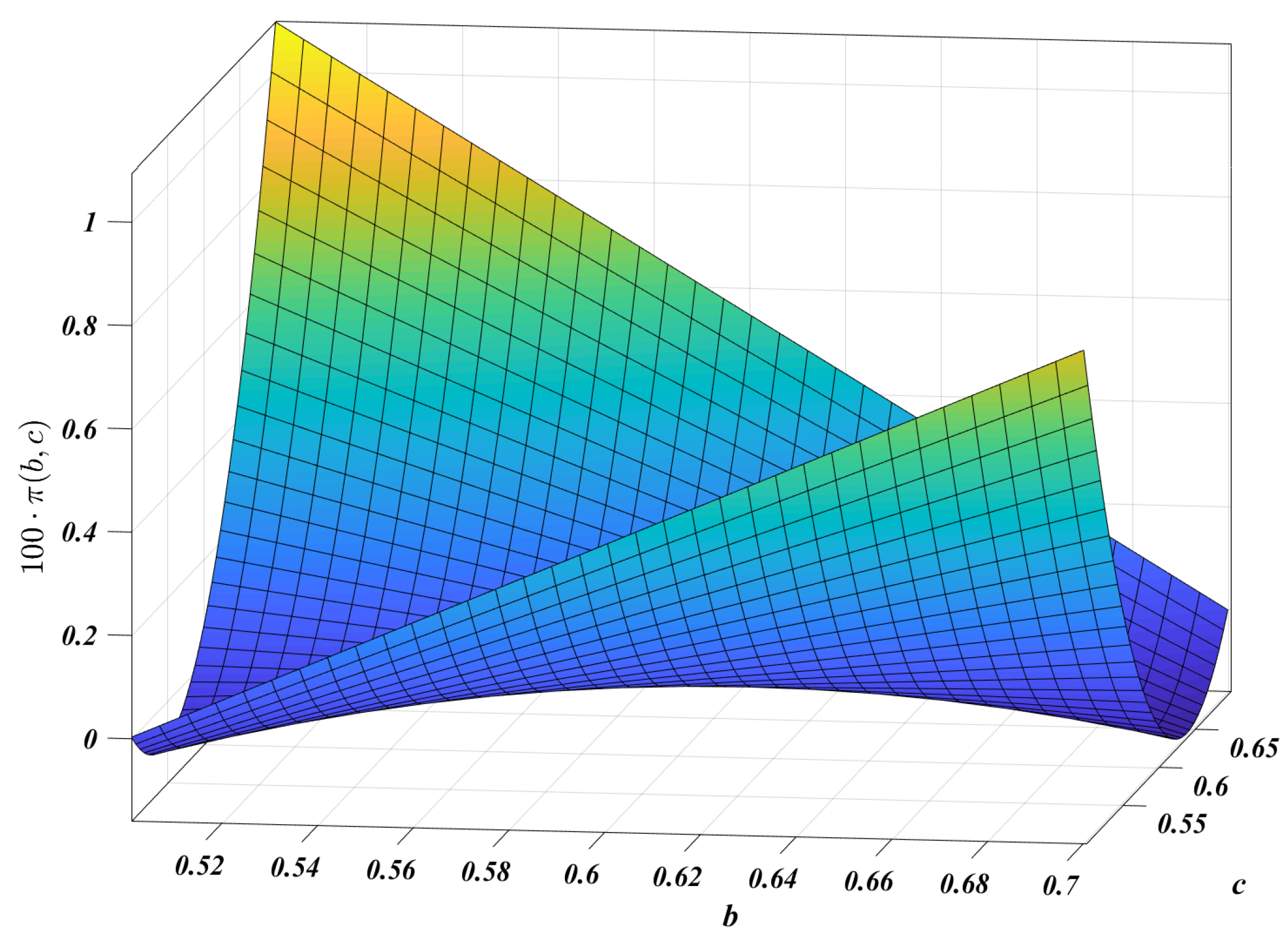
Thus, we will work with the simplified payoff kernel
which is the compound-growth rate of . Since is concave (in fact, linear) in b and convex in c, the saddle point is characterized by the first-order condition Taking the gradient with respect to b, we get the equation
This is precisely the first-order condition that defines the Kelly rule for jump diffusions. The equation has a unique solution that serves to define . In just a moment, we will take the gradient of with respect to c, by using the product rule. To this end, we let D denote the differential (an matrix) of the mapping of into itself. We have
We note that D is negative semi-definite, since it is the Hessian matrix of the concave function This being done, we apply the product rule and get the first-order condition
where is the identity matrix (e.g., the differential of ). Now, note that the matrix is negative definite (therefore invertible), since it is the sum of a negative definite matrix and a negative semi-definite matrix. Thus, from the equation we obtain . This proves that the unique saddle point is for both players to use the Kelly rule for jump diffusions, and that the value of the simplified game (with kernel ) is 1.
4. Solution of the Investment -Game
On account of the fact that the unique saddle point of is to set and equal to the Kelly rule, we have the inequalities
which hold for all . Thus, when the numerator player uses the Kelly rule it guarantees that the expected payoff is ≥1, and when the denominator player uses the Kelly rule it guarantees that the expected payoff is ≤1. With these guarantees in mind, we proceed to solve the general investment -game. First, we need a definition.
Definition 4.
For any increasing function , the “ primitive -game,” with value , is the two-person, zero-sum game with payoff kernel , where player 1 chooses a fair randomization and player 2 chooses a fair randomization . The value of the primitive ϕ-game is . The random wealths and are independent of each other.
We should stress to the reader that this definition tacitly assumes the existence of a saddle point of the primitive -game, e.g., we have assumed the equality
of the lower and upper values of the game. For more on this point, we refer the interested reader to Bell and Cover (1988).
Theorem 2.
The investment ϕ-game has the same value as the primitive ϕ-game. In equilibrium, both players use the Kelly rule for jump diffusions, and the players use the same fair randomizations that solve the primitive ϕ-game.
Proof.
The proof given in Garivaltis (2018) carries over to the more general case of several jump diffusions. We start by showing that for any fair randomization and any rebalancing rule , where is the Kelly rule. Note that is a fair randomization, since . Thus, since , is Player 1’s maximin strategy in the primitive -game, we have .
Similarly, we show that for any fair randomization and any rebalancing rule , where is the Kelly rule. Note that is a fair randomization, since . Thus, since , is Player 2’s minimax strategy in the primitive -game, we must have .
Thus, we have shown that guarantees that the expected payoff is and guarantees that the expected payoff is when and are equal to the Kelly rule and are the equilibrium strategies from the primitive -game. This proves the theorem. □
5. Examples
To close the paper, we simulate some gameplay for a market with a single stock that diffuses according to the parameters , , and . We assume a risk-free rate of , and that jumps arrive at an expected rate of per year. On jumps, the gross-returns will be distributed according to “Shannon’s Demon” (Poundstone 2010 [10]), e.g.,
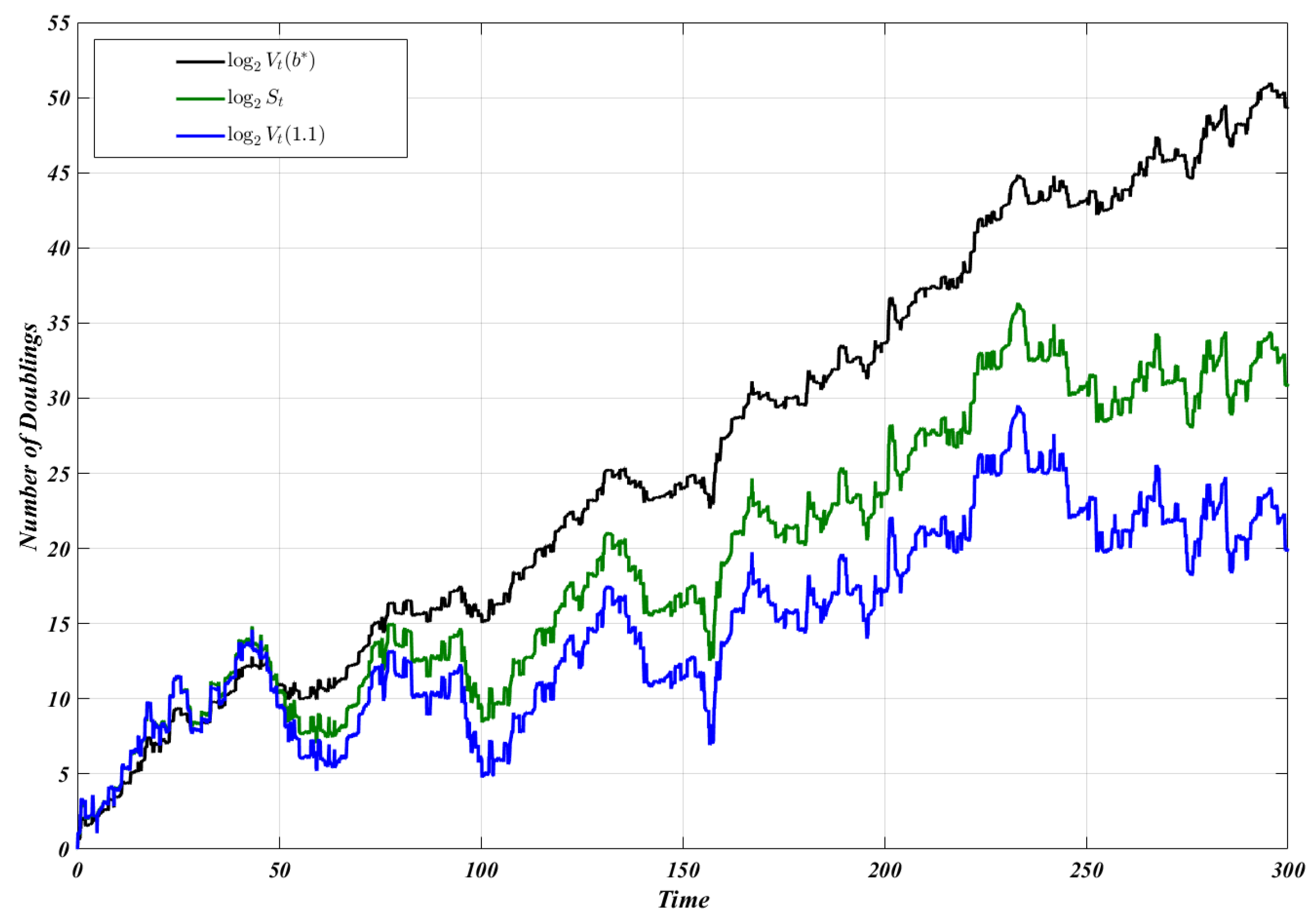
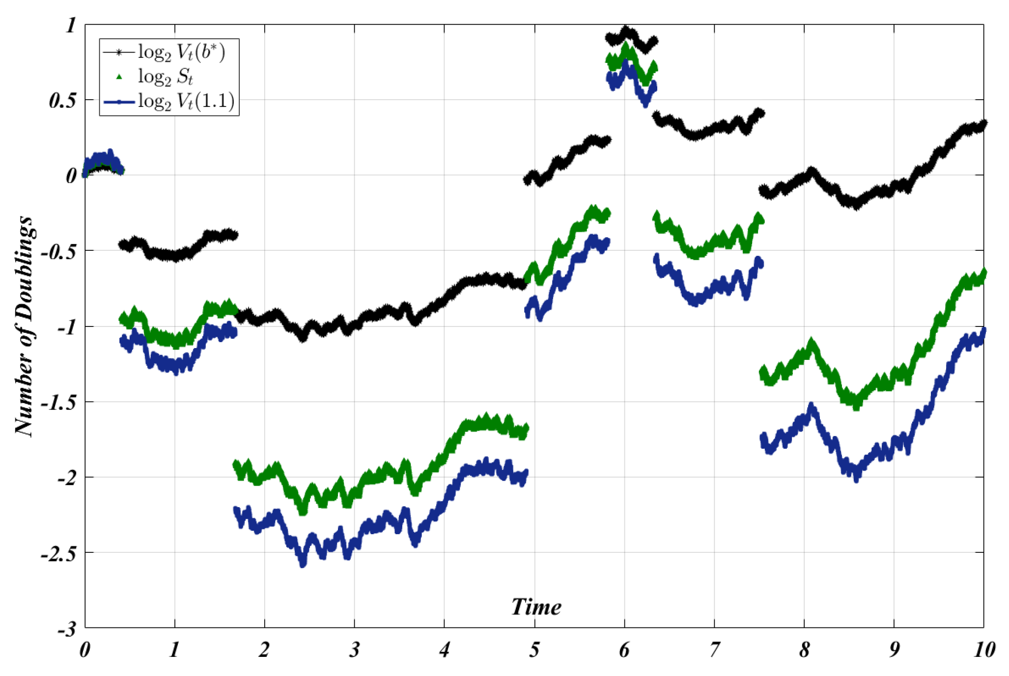
meaning that the stock price either doubles or gets cut in half, each with equal probability. If one could anticipate these jumps, then the growth-optimal policy would be to put the instant before each jump, achieving long-run capital growth of per jump. During diffusion (before and after the jumps), the correct policy would be to set , achieving a growth rate of a year, for a total of annually. In our game, however, the jumps are unanticipated; the rule goes bankrupt just as soon as . In fact, . The Kelly rule for jump diffusions is , for a yield of per year. The saddle is plotted in Figure 1. We compare this to the sub-optimal behavior of two other players: a player who uses (buy and hold) and a daring player who uses A sample path for years is plotted in Figure 2. A (different) sample path for years is shown in Figure 3.
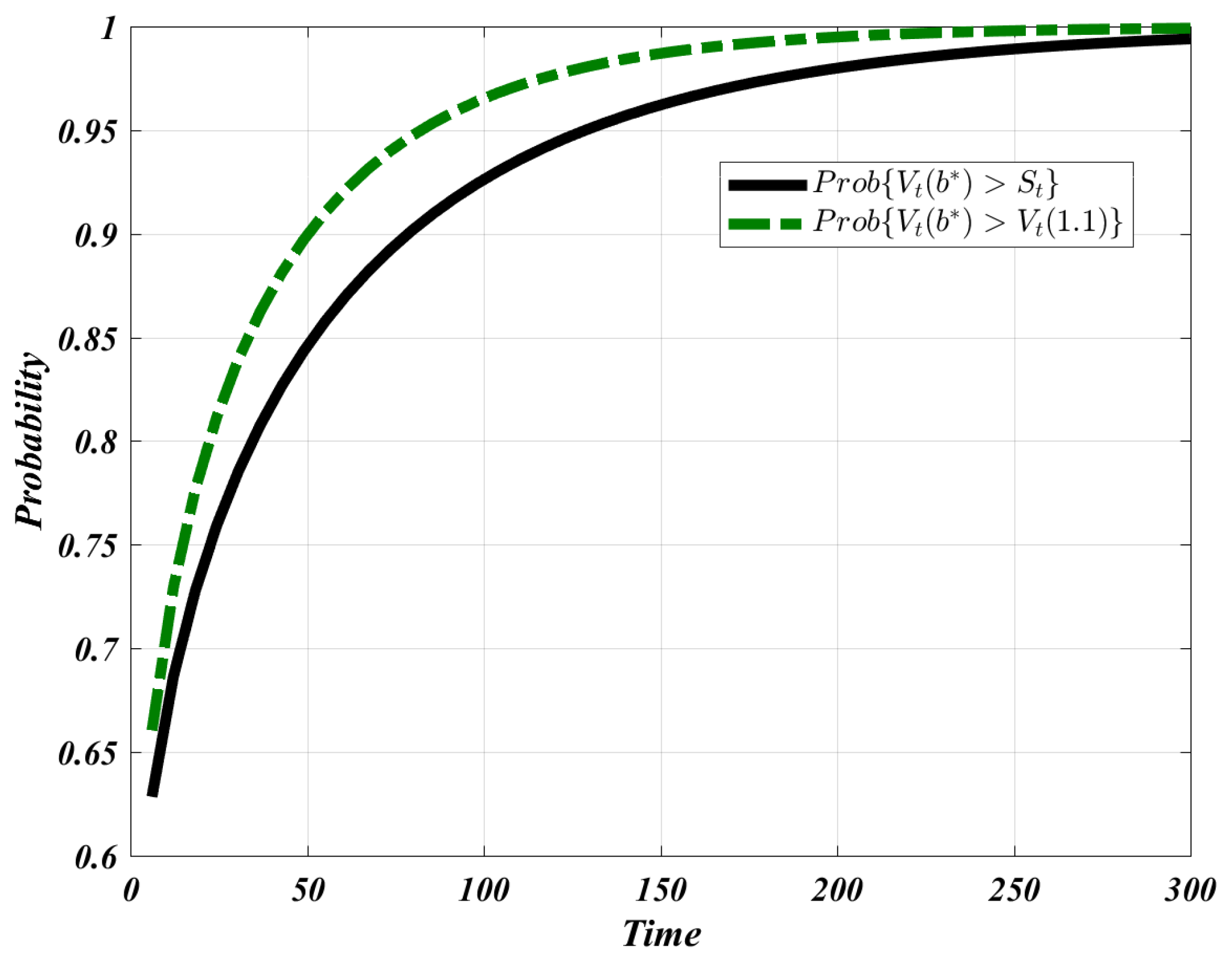
Let denote the number of times the stock jumps upward over the interval , where is the number of times it jumps downward. We let . Then we have
where, for ,
where is the cumulative normal distribution function and denotes the growth rate of b during diffusion. The outperformance probabilities for this particular experiment () are plotted in Figure 4 for .
6. Conclusions
This paper formulated and solved a two person trading game in continuous time that generalizes Garivaltis [5] to the case of several jump diffusions. Following a train of thought initiated by Bell and Cover [1,3], we solved a leveraged “investment -game” where the object is to outperform the other investor with respect to some more or less arbitrary criterion of relative performance.
At the start of the game, each player makes a “fair randomization” of the initial dollar by exchanging it for a random wealth whose mean is at most 1. Each player then deposits the resulting capital into some continuously rebalanced portfolio (or fixed-fraction betting scheme) that is adhered to over a fixed interval of time. We showed that the unique saddle point of the expected final wealth ratio is for both players to use the Kelly rule for jump diffusions, in conjunction with appropriate fair randomizations that are completely determined by the criterion .
From time immemorial Kelly [2], the Kelly rule has been defined by maximizing the almost sure asymptotic continuously-compounded growth rate of one’s bankroll. However, the above analysis shows that, even for an egotist whose sole objective is to outperform his peers over very short time periods, the Kelly rule for jump diffusions is the correct behavior. On the one hand, although the investor knows the distribution of jump returns, he cannot anticipate their exact arrival times. Thus, his only recourse is to build a portfolio that is continuously ready to perform well when the lightning strikes. On the other hand, he wants a trading strategy that performs well during purely diffusive movements of security prices. The Kelly rule is the sweet spot that perfectly balances these two concerns.
Thus, the present paper constitutes a direct generalization of both Bell and Cover [3] and Garivaltis [5]. If the expected jump arrival rate is zero, we specialize to Garivaltis [5]. If the diffusion parameters are zeroed out (meaning that stock prices do not change during “diffusion”), then we get a leveraged version of Bell and Cover’s original [3] game-theoretic optimal portfolios, albeit with the proviso that the players must watch the paint dry as they wait for jumps to arrive. If everything is zeroed out, then we get the “primitive -game” of choosing fair randomizations that constitute a saddle point of .
Funding
This research received no external funding and the Article Publishing Charge was funded through the Knowledge Unlatched initiative.
Conflicts of Interest
The author declares no conflict of interest.
References
- Bell, R.M.; Cover, T.M. Competitive Optimality of Logarithmic Investment. Math. Oper. Res. 1980, 5, 161–166. [Google Scholar] [CrossRef]
- Kelly, J.L. A New Interpretation of Information Rate. Bell Syst. Tech. J. 1956, 35, 917–926. [Google Scholar] [CrossRef]
- Bell, R.; Cover, T.M. Game-Theoretic Optimal Portfolios. Manag. Sci. 1988, 34, 724–733. [Google Scholar] [CrossRef]
- Samuelson, P.A. Why We Should Not Make Mean Log of Wealth Big Though Years to Act Are Long. J. Bank. Financ. 1979, 3, 305–307. [Google Scholar] [CrossRef]
- Garivaltis, A. Game-Theoretic Optimal Portfolios in Continuous Time. Econ. Theory Bull. 2018, 1–9. [Google Scholar] [CrossRef]
- Merton, R.C. Option Pricing When Underlying Stock Returns are Discontinuous. J. Financ. Econ. 1976, 3, 125–144. [Google Scholar] [CrossRef]
- Bernhard, P.; Engwerda, J.C.; Roorda, B.; Schumacher, J.M.; Kolokoltsov, V.; Saint-Pierre, P.; Aubin, J.P. The Interval Market Model in Mathematical Finance: Game-Theoretic Methods; Springer Science & Business Media: Berlin, Germany, 2012. [Google Scholar]
- Berge, C. Topological Spaces; Oliver and Boyd: Edinburgh, UK, 1963. [Google Scholar]
- Wilmott, P. Paul Wilmott Introduces Quantitative Finance; John Wiley & Sons: Hoboken, NJ, USA, 2001. [Google Scholar]
- Poundstone, W. Fortune’s Formula: The Untold Story of the Scientific Betting System that Beat the Casinos and Wall Street; Hill and Wang: New York, NY, USA, 2010. [Google Scholar]
Figure 1.
Payoff kernel for the parameters . The saddle point is .

Figure 2.
A sample path in the large. .

Figure 3.
A (different) sample path in the small. .

Figure 4.
Outperformance probabilities over different game lengths for the parameters .

© 2019 by the author. Licensee MDPI, Basel, Switzerland. This article is an open access article distributed under the terms and conditions of the Creative Commons Attribution (CC BY) license (http://creativecommons.org/licenses/by/4.0/).
Share and Cite
MDPI and ACS Style
Garivaltis, A. Game-Theoretic Optimal Portfolios for Jump Diffusions. Games 2019, 10, 8. https://0-doi-org.brum.beds.ac.uk/10.3390/g10010008
AMA Style
Garivaltis A. Game-Theoretic Optimal Portfolios for Jump Diffusions. Games. 2019; 10(1):8. https://0-doi-org.brum.beds.ac.uk/10.3390/g10010008
Chicago/Turabian StyleGarivaltis, Alex. 2019. "Game-Theoretic Optimal Portfolios for Jump Diffusions" Games 10, no. 1: 8. https://0-doi-org.brum.beds.ac.uk/10.3390/g10010008
Note that from the first issue of 2016, this journal uses article numbers instead of page numbers. See further details here.