Team Production and Esteem: A Dual Selves Model with Belief-Dependent Preferences


Institute of Management and Economics, Clausthal University of Technology, Julius-Albert-Str. 2, 38678 Clausthal-Zellerfeld, Germany
Games 2019, 10(3), 33; https://0-doi-org.brum.beds.ac.uk/10.3390/g10030033
Submission received: 27 May 2019
/
Revised: 20 July 2019
/
Accepted: 10 August 2019
/
Published: 14 August 2019
(This article belongs to the Special Issue Advances in Behavioral Economics: Empathy and Happiness)
Abstract
:We propose a dual selves model to integrate affective responses and belief-dependent emotions into game theory. We apply our model to team production and model a worker as being composed of a rational self, who chooses effort, and an emotional self, who expresses esteem. Similar to psychological game theory, utilities depend on beliefs, but only indirectly. More concretely, emotions affect utilities, and the expression of emotions depends on updated beliefs. Modeling affective responses as actions chosen by the emotional self allows us to apply standard game-theoretic solution concepts. The model reveals that with incomplete information about abilities, workers only choose high effort if esteem is expressed based on interpersonal comparisons and if the preference for esteem is a status preference.
Keywords:
affective responses; belief-dependent motivations; emotions; psychological game theory; team production; status preferences; esteemJEL Classification:
C7; D03; D21; D8; M51. Introduction
Emotions can have important consequences in a wide variety of economic and social interactions. Our paper presents an approach to integrate affective responses, like the expression of emotions, into game-theoretic models. In particular, we focus on one particular anticipatory emotion, esteem, and illustrate the interplay between players’ information and the effect of emotions.1
Different approaches to integrate individuals’ preferences over emotions and the expression of emotions into game theory can be distinguished.
One approach would be to assume that players correctly anticipate the emotions associated with each possible outcome of the game. Then, we could integrate emotions by adjusting the payoffs, so that the effect of emotions is reflected in the game’s adjusted payoffs. Since in the description of the game, payoffs are given, the impact of emotions has to be independent of the game’s solution. This turns out to be problematic in games of incomplete information where emotions are belief-dependent.
Another approach is to model affective responses explicitly as additional moves. The expression of emotions is part of a player’s strategy so that the information structure and the corresponding beliefs can explicitly be taken into account. In this approach, the expression of emotions stems from a rational cost-benefit calculus, which seems paradoxical because in general, emotions cannot be supplied intentionally (for a more detailed discussion, see [6,7]).
Our approach differs from the two just-mentioned approaches. It belongs to the group of dual selves models [8,9,10,11], which conceptualize a player’s behavior as being determined by the interaction between a rational and an emotional self. This does not imply that there are two separate systems determining an individual’s behavior. Rather, the interpretation of our model is more functional (see also Sloman [12], 1996, and Frank et al. [13], 2009). Our model allows us to model emotional decisions explicitly, like the expression of esteem, while taking the game’s information structure into account. Since each player consists of a rational and an emotional self, emotions are not expressed based on a rational cost-benefit calculus.
Consider a software engineer who presents a smart solution for a difficult problem. By presenting a smart solution, she/he signals her/his ability. The members of her/his team acknowledge the high quality of her/his work by nodding in agreement or by the widening of eyes as a sign of surprise. Using such affective responses, the team members express their emotions, in this case, esteem towards the software engineer.2 Eventually, the engineer’s utility increases in response to the esteem expressed by her/his team members. Esteem is not supplied intentionally. Rather, the expression of esteem is based on the evaluation of the engineer’s effort and ability. Of course, the members of the team can intentionally decide how much attention to pay or whether to express or to withhold esteem. The important point, however, is that the expression of esteem is a judgment formed in an emotion-based, rather than in a reason-based process. Using a dual selves model allows us to capture this distinction between emotion-based and reason-based decisions.
In our model of team production, esteem is expressed after workers have chosen their efforts. That is, effort choices are the stimuli, which workers evaluate, and to which they react by expressing esteem. The expression of esteem is an affective response, which translates a stimulus-evoked feeling into evaluative behavior.
Our approach is related to psychological game theory [14], in which utilities are belief-dependent and beliefs are updated as the game unfolds [1,15,16,17]. This is also the case in our model. Our model differs from several psychological game theory models (e.g., [18,19]) in the following respect. The work in [18] was a theory-driven experimental paper, which focused on how communication affects beliefs. In [19], framing affects subjects’ prior beliefs and first- and second-order beliefs affected utilities. In our model, prior beliefs are exogenously given, and the focus is on the interplay between players’ information and the effect of belief-dependent emotions on effort. The expression of esteem depends on abilities, which captures the idea that for a given outcome, the amount of esteem expressed is inversely related to the ability of the individual whose actions caused the outcome. With incomplete information about abilities, the amount of esteem Player 1 expresses towards Player 2 depends on Player 1’s beliefs about Player 2’s ability. Consequently, the utility Player 2 expects to derive from esteem expressed by Player 1 depends on Player 2’s second-order beliefs. Using a dual selves model allows us to model the updating of beliefs in a sensible way.3
The first contribution of this paper is an argument for modeling. When affective responses and the corresponding emotions depend on (updated) beliefs, our model can be used to analyze affective responses using standard game-theoretical methods. The literature following Geanakoplos et al. [14] and Battigalli and Dufwenberg [16] has shown how to integrate belief-dependent emotions into game-theoretic models. In [14,16], the focus was on a new solution concept (psychological sequential equilibrium), while the framework developed in this paper relies on standard solution concepts (perfect Bayesian equilibrium). This is the first advantage of our dual selves model. Secondly, our model extends psychological game theory by explicitly modeling the expression of emotions as affective responses. A third advantage is that it describes two different functional processes, bringing it closer to the literature on cognitive psychology [10]. While the rational self describes a cognitive process, the emotional self describes a process that is largely unconscious. Of course, a disadvantage of our dual selves model is that it results in a larger model with twice as many players. However, with the view on the aim of reaching a better understanding of the role of belief-dependent emotions in strategic interactions, our model can be applied not only to esteem, but to a wide range of expected emotions.4
The second contribution results from the application of our model. By introducing esteem into the problem of team production, our model generates novel predictions. The model shows that if information about abilities is private, workers will only choose high effort if the social comparison and the status condition are fulfilled. The social comparison condition holds if esteem is expressed based on interpersonal comparisons; and the status condition holds if the preference for esteem is a status preference. We will discuss both conditions in more detail below.
We proceed as follows. In Section 2, we introduce a reference model without esteem and extend it step by step in order to model both the expression of and workers’ preferences for esteem adequately. We solve the model for complete and incomplete information about abilities and summarize the model’s main results. In Section 3, we discuss our model in light of the related empirical evidence and conclude by arguing that dual selves models are suitable models for integrating affective responses into game theory.
2. Team Production with Esteem Incentives
In many production processes, output is a function of several workers’ efforts. Individual effort is rarely contractible; hence, contracts are incomplete, and free-riding can lead to inefficiencies. We consider a setting in which individual effort is not contractible, but in which mutual monitoring is possible. As an example, think of two workers, who can monitor each other because they share an office. In such a setting, esteem incentives result in peer pressure if workers compare each other. This in turn, can generate productivity spillovers.
Mas and Moretti [24] studied the productivity of cashiers and found evidence for productivity spillovers driven by peer pressure. In particular, they found that the introduction of a highly-productive worker increases the productivity of colleagues who could observe the productive worker. The increase in productivity is higher for workers who interact more frequently. Mas and Moretti [24] argued that in infrequent encounters, workers are less receptive to peer pressure because they do not know each others’ productivities (134, 141). These empirical findings can be rationalized within our model, which states that for moderate social comparisons, esteem leads to efficiency gains only if workers know each others’ abilities.
We take the concept of esteem to summarize all non-material incentives one worker receives from her/his colleagues. Taking it as given that workers have a status preference for esteem, we analyze the interplay between esteem incentives and team production.
Related to our model as well are several theoretical contributions, which analyze optimal contracting between a principal and multiple agents with social preferences [25,26,27,28]. In contrast to our model, in [25,26,27], agents preferences depended only on outcomes and not on beliefs. Only in [28], agents preferences were belief dependent.
2.1. A Reference Model without Esteem
Consider two workers being involved in team production, which we model as a two-stage game. In the first stage, nature decides each worker’s type, which we interpret as ability. Ability can be high (type H) or low (type L) with . With probability p (), a worker has high (low) ability. There are two workers with abilities and . Assume that the workers’ types are independent and that p, L, and H are common knowledge. Types can be common knowledge (Section 2.3) or private information (Section 2.4).
In the second stage, workers simultaneously choose effort, which is observable, but not verifiable. Type L workers always choose low effort and incur the cost of effort of c.5 Type H workers choose between low and high effort, . We normalize the cost of effort for working below full potential at zero and use to denote the cost of choosing high effort.
Since low types always choose , we focus on high types. Let denote i’s effort when his/her own ability is H and others’ ability is y. Worker i’s strategy consists of a vector defining an action for each distribution of abilities. Let be the set of all four pure strategies for a high-type worker in the game with complete information.
The payoff from team production is given by the sum of efforts. Workers have preferences over monetary income and cost of effort. We assume that preferences are separable and given by:
In Equation (1), denotes i’s choice of effort for a given distribution of abilities, i.e., if and and if . The function is an indicator function that equals one if effort equals type, i.e., only for high-ability workers who chose low effort, the cost of effort is zero.6
If abilities are private information, a worker cannot condition her/his effort on the other worker’s ability. Since low types always choose low effort, a worker’s strategy is her/his effort when she/he has high ability, . Let be the set of all pure strategies. With abilities being private information, the utility function is:
In Equation (2), the abilities are private information, and denotes i’s choice of effort when her/his own ability is high.
We assume , so that each worker has an incentive to shirk, but welfare is maximized when both workers choose not to shirk. With public and private information about abilities, always choosing low effort is the dominant strategy in this reference model.
2.2. Incorporating Affective Responses
To consider affective responses, we add a third stage. At the beginning of the third stage, workers are informed about chosen efforts. Both workers’ emotional selves, which we introduce below, react to this information by publicly expressing esteem. The expression of esteem is modeled as an affective response, which we describe in Section 2.2.1. When solving the model, we assume that workers anticipate affective responses and take them into account when choosing effort. The existence of this third stage has no effect on the strategy sets (R and ), but as we will see, it can affect the game’s equilibrium if workers have a preference for esteem.
Note that our model relies on the assumption that esteem is expressed publicly. As noted above (Section 1), esteem is expressed unintentionally through the psychological expression of emotions, like smiling or nodding. In work environments, in which these expressions are highly visible (e.g., shared offices allowing frequent and open communication), the assumption that esteem is expressed publicly is likely to hold. Our model applies to such environments.7
2.2.1. Expressing Esteem
We assume that esteem is expressed simultaneously and that there is no direct cost associated with the expression of esteem.8 The strength of the affective response depends not only on a worker’s relative effort, but also on the relative effort of some reference group [7] (pp. 80–81). Since we consider a team of two workers, we take the other worker as the reference group. The stimulus prompted by the choices of effort depends on both workers’ relative efforts. Assuming linearity, i expresses esteem according to:
where . is i’s expectation about j’s ability conditional on j’s effort. Depending on the parameter , we can distinguish two different affective responses.
No social comparison (): Without social comparison, esteem is an incentive that is supplied in response to the other worker’s choice of effort. The affective response is nonnegative and proportional to the other worker’s relative effort, . It is independent of the effort level chosen by the worker whose affective response we consider () because the social comparison condition is not fulfilled, i.e., .
Social comparison (): Esteem is an incentive supplied in response to one’s own and the other workers’ choice of effort. It will be stronger if j’s relative effort is higher or if i’s relative effort is lower, implying that the difference between j’s and i’s relative effort is higher. The parameter indicates the importance of the comparison to the reference group.
In Equation (3), we assume a negative relationship between esteem and ability conditional on effort. This captures the idea that a given level of effort generates higher esteem if it comes from a worker with lower ability. To illustrate this assumption, we go back to the example mentioned in the Introduction. Assume that there is a software engineer A who has low ability because she is new in the profession. Furthermore, there is software engineer B, who has high ability because she has several years of experience. Now, if both make the same contribution, A’s contribution triggers more esteem because A is doing the best she can, while B could have done better.
Because types are given and efforts are chosen in Stage 2, Equation (3) contains no choice variable. The expression of esteem can be thought of as an affective response triggered by a worker’s emotional self. The behavior of each emotional self is specified by Equation (3), which reflects the fact that emotions are expressed based on intuitive and fast processing of information, rather than slow, reason-based processing of information.9 Although the expression of esteem is no choice in the game-theoretic sense, it affects payoffs and hence can affect the game’s equilibrium, which we will discuss next.
2.2.2. Workers’ Preferences for Esteem
The preceding section describes the supply of esteem. To model the demand for esteem, we extend the utility functions introduced in Section 2.1. The preference for esteem is a status preference. A player’s status depends on relative esteem, i.e., the amount of esteem she/he receives compared to the amount of esteem that the other player receives.10
Assume that i’s preferences are given by . The strictly increasing and concave function:
gives the utility resulting from esteem. The preference for esteem is a status preference, and the parameter measures the strength of this status preference. Higher values imply stronger status effects.
The function () denotes esteem expressed by i (j), which depends on both workers’ relative efforts, as described in Section 2.2.1. The parameter k is a constant and represents the amount of esteem each worker receives from exogenous sources.11
Substituting for , the utility function can be written as:
if abilities are common knowledge and:
if abilities are private knowledge. The terms and denote i’s expectation about and .
We implicitly assume that esteem utility is an emotion that is experienced at the end of Stage 3, after esteem is expressed. Hence, expectations about esteem are relevant for workers’ choices of effort. We assume that the expression of esteem takes place against the backdrop of specific organizational practices known to all workers, so that workers can anticipate esteem correctly. In other words, esteem is a component of the expected consequences of the choice of effort.
Note that if the social comparison condition is fulfilled (), there are two interpersonal or social comparisons. First, there is a social comparison in the expression of esteem, whose strength is captured by . This comparison is at work when workers express esteem, regardless of how esteem affects utilities. Second, there is a social comparison in the utility derived from esteem (captured by ). This comparison is at work only if workers have a status preference for esteem (regardless of how esteem is expressed).12 Furthermore, note that we assume complete information about preferences, i.e., the parameters k, , and are common knowledge. In Section 2.3, we assume that workers’ abilities are also common knowledge, and in Section 2.4, we assume that there is uncertainty with respect to workers’ abilities.
2.3. Abilities Are Common Knowledge
In this section, we show that when abilities are common knowledge, the expression of esteem is not dependent on beliefs. There is no need for a dual selves model. Rather, we can modify the payoffs and solve the model. Esteem is anticipated correctly, so that the expression of esteem changes payoffs. New payoffs are given by Equation (4), where we can replace the conditional expectation by the actual ability, . Substituting and into the utility function yields utility as a function of effort levels and abilities.
Let:
is the increase in utility from esteem if a worker increases her/his effort while the other worker exerts less than maximal effort. Similarly, is the increase in utility from esteem if a worker increases her/his effort while the other worker exerts maximal effort. The variable z denotes the opportunity cost of increasing effort. For all and , . and increase in and , while z does not depend on these parameters. For given abilities and cost of effort, the set of equilibria is completely characterized by and .
Throughout this paper, we focus on symmetric equilibria in pure strategies. The focus on symmetric equilibria is sensible because ex ante, all workers are homogeneous and face the same decision problem. The equilibria are summarized in Propositions 1–3 and illustrated in Figure 1. For a derivation, see Appendix A.
Proposition 1.
With abilities being common knowledge, there exists an equilibrium in pure strategies, in which both workers choose high effort if the social comparison condition is strong (β is high), or if status concerns are strong (α is high) because, then . The equilibrium is unique if .
Proposition 2.
With abilities being common knowledge, there exists an equilibrium in pure strategies, in which both workers choose low effort if the social comparison condition is weak (β is low), and if status concerns are weak (α is low) because, then . The equilibrium is unique if .
Proposition 3.
With abilities being common knowledge and for medium values of α and β, there exist two equilibria in pure strategies. This is the case if . Effort levels are strategic complements so that in equilibrium, high ability workers coordinate on either the low effort or the high effort equilibrium. The high effort equilibrium is Pareto dominant (for a proof, see Appendix A).
In Figure 1, the solid line represents all pairs so that . Points above (below) the solid line are combinations of and for which (). The dashed line represents all pairs so that . Points above (below) the dashed line are combinations of and for which (). The lines do not cross because for given values of , with strict equality only if .
Every combination of and can be represented by a point in Figure 1. If the point lies in region (3), this combination of parameters corresponds to the low effort equilibrium. For low values of and , workers always choose low effort, regardless of the distribution of abilities.
If the point () lies in Region (1), this combination of parameters corresponds to the high effort equilibrium. Both workers choosing high effort is a unique equilibrium if or are high.
Points in Region (2) correspond to combinations of and for which two pure strategy equilibria exist. The equilibria differ only in the choice of effort if both workers have high abilities. A worker with high ability always chooses high effort if the other worker has low ability. If both workers have high abilities, each worker’s best response is to choose the same amount of effort as the other worker. Effort levels are strategic complements so that workers have to coordinate on either the low effort or the high effort equilibrium.13
Note that when the status condition is fulfilled and strong enough () or when the social comparison condition is fulfilled and strong enough (), each worker will choose high effort, regardless of the other worker’s ability. In order to get to the high effort equilibrium, it is sufficient if only one of the two social comparisons is strong enough.
2.4. Incomplete Information about Abilities
In this section, we show that with incomplete information about abilities, the expression of esteem is dependent on beliefs. Consequently, esteem enters the utility function as a belief-dependent motivation. In order to capture how esteem depends on updated beliefs, we propose a dual selves model.
Assume that after abilities are drawn, workers do not learn about others’ abilities. Player i, who expresses esteem, knows his/her own type (), but does not know the others’ type (). As before, i expresses esteem according to Equation (3). When maximizing utility, i has to form expectations about . Taking expectations, we write Equation (3) as:
where is i’s second-order belief about her/his own ability. We assume that . Equation (7) describes i’s expectation about esteem expressed by j. Since esteem is expressed after effort levels are observed, expectations are conditional on effort.
For given conditional expectations, esteem utility is given by with:
Note that through the term , expected esteem utility depends on a worker’s own ability. Although abilities are private information, the amount of esteem utility a worker receives depends on her/his own ability, in addition to each worker’s beliefs about the others’ ability.
The expression of esteem is modeled as an affective response whose strength is determined by types and effort levels. Although affective responses determine the game’s payoffs, the expression of esteem is not modeled as a choice. In the model with complete information, this was not a problem because abilities were common knowledge, so that the expression of esteem was independent of expectations. With incomplete information, however, effort choices can signal abilities, so that the expression of esteem depends on conditional expectations. More precisely, we need conditional expectations at the end nodes where the game’s payoffs are specified. Here, we run into a problem because standard solution concepts only contain well-defined beliefs at the player’s information sets, but not at the end nodes.
To solve this problem, we propose a dual selves model in which each worker consists of a rational and an emotional self, who are connected in the sense of sharing the same information. While the rational self’s behavior is derived from a utility function defined over expected payoffs and esteem, the emotional self’s behavior represents an automatic affective response. The affective response can, in principle, also be derived from utility maximization by specifying a utility function for the emotional self. In the context of our model, a plausible utility function would be a negative quadratic loss function, , as it is often assumed in the literature on strategic information transmission (e.g., [33], p. 1440).14
Using the dual selves model, we model the same decision situation as before, but in a different way. In the dual selves model, both rational selves simultaneously choose efforts, as before. Then, esteem is expressed simultaneously by both workers’ emotional selves. More precisely, the emotional self chooses her/his conditional expectation about the others’ ability, maximizing her/his payoff, which is defined by the quadratic loss function. Note that the emotional self’s choice of her/his conditional expectation does not correspond to an intentional decision of the worker. Rather, it is a game-theoretical representation of the behavior of the worker’s emotional system.
The conditional expectation chosen by the emotional self determines the affective response (Equation (7)) and the corresponding esteem utility (Equation (8)). By explicitly modeling the emotional selves, the nodes at which esteem is expressed are no longer end nodes. Hence, we can apply standard game-theoretic methods. Using backward induction, we can now solve the game by starting with the last decision (the expression of esteem by both worker’s emotional selves).15
2.4.1. Pooling Equilibrium
Assume that in equilibrium, both workers choose low efforts, regardless of their abilities. This is a pooling equilibrium because effort choices reveal no information about workers’ abilities.
Part of the equilibrium is a consistent system of beliefs that assigns probabilities to all decision nodes in the game, such that the probabilities within each information set sum up to one. For i’s emotional self, there are two information sets, one for and one for . She/he cannot distinguish between the nodes within each information set and puts the same probability on each node. However, if j’s rational self deviates and she/he chooses , she/he has revealed her/his type, and i’s emotional self knows exactly which node in the information set has been reached. Hence, i’s emotional self puts a probability of one on one node in the information set if j deviates. For the sake of simplicity, we directly specify the relevant conditional expectations:16
where is expected ability. In equilibrium, conditional expectations are . These conditional expectations are the emotional selves’ choices and determine the expression of esteem. Equation (8) gives esteem utility, which (in equilibrium) is:
In the rest of this section, we assume that Worker 1 has high ability () because only workers with high ability can deviate by choosing high effort. In equilibrium, 1’s expected utility is given by:
She/she can deviate by increasing her/his effort to H. Because of the deviation, Worker 2 knows for sure that Worker 1 has high ability. Worker 2’s conditional expectation about Worker 1’s ability is equal to her/his true ability, . This changes esteem utility to:
and yields utility:
For Worker 1, deviation increases utility if:
with:
By symmetry, the same reasoning holds for Worker 2. Hence, effort choices and the corresponding beliefs, which determine and , constitute a perfect Bayesian equilibrium if .
2.4.2. Separating Equilibrium
Assume that is the equilibrium strategy profile. We call this the separating equilibrium because in equilibrium, low ability workers choose low efforts and high ability workers choose high efforts. In equilibrium, conditional expectations are given by:
Equation (8) simplifies to:
As before, we assume that Worker 1 has high ability. Worker 1’s expected utility is given by:
Here, is the net utility from Worker 1’s effort and is the expected utility from the other worker’s effort. Worker 1 can deviate by decreasing her effort to L, which yields utility:
The strategy profile and the corresponding beliefs, which determine and , constitute a perfect Bayesian equilibrium if:
with:
Only if and are positive, a high ability worker achieves a higher monetary payoff, but lower esteem utility by deviating to low effort. The deviation does not affect expectations, but because i’s relative effort appears in Equation (8), esteem decreases. We call this the guilt effect: although Worker 2’s conditional expectation about 1’s ability is independent of 1’s actual effort (observing is not informative), esteem utility is lower because the strength of the emotional self’s affective response is inversely related to her/his ability. Although the expectations remain constant, a deviation decreases 1’s esteem utility because she/he knows that she/he could have chosen higher effort. This definition of guilt is similar to Kandel and Lazear [23], who stated that “[g]uilt is internal pressure, whereas shame is external pressure” (p. 806). It is also similar to the definition of simple guilt in [37], according to which guilt is “the extent to which he [a player] lets another player down” ([37], p. 171).
2.4.3. Characterization of Equilibria with Incomplete Information about Abilities
In the game with incomplete information of abilities and for given abilities and costs of effort, the set of equilibria is completely characterized by Equations (10) and (12) and the corresponding beliefs. For reasonable assumptions, .17 We now can distinguish two cases.
First, consider the case when or . This implies that , so the separating equilibrium cannot exist. The pooling equilibrium is the unique pure strategy equilibrium if . One can show that if , increases in , and if , increases in . This means that the pooling equilibrium exists if the social comparison condition or status concerns are strong enough.
Second, consider the case when and . In this case, both and are strictly positive and increase in and . When and are high enough, , so that the separating equilibrium is the unique pure strategy equilibrium. The equilibria are summarized in Proposition 4 and illustrated in Figure 2.
Proposition 4.
With incomplete information about abilities, the separating equilibrium exists only if both and . When or , only the pooling equilibrium exists.
In Figure 2, the solid line represents all pairs so that . Points above (below) the solid line are combinations of and for which (). The dashed line represents all pairs so that . Points above (below) the dashed line are combinations of and for which ().
For low values of and , z exceeds and , and workers always choose low effort. In Figure 2, points in Region (3) correspond to this pooling equilibrium.
For medium values of and , , neither Equation (10) nor Equation (12) is fulfilled, so that there exists no equilibrium in pure strategies. In Figure 2, points in Region (2) are combinations of for which this is the case.
For high values of and , , and workers will always choose high effort. Combinations of and in Region (1) of Figure 2 correspond to this separating equilibrium.
2.5. The Model’s Main Results
Result 1: The socially-optimal outcome occurs when high ability workers always choose high effort. With complete information about abilities, the socially-optimal outcome is obtained if or are high enough. This means that only one of the social comparisons (the status condition and the social comparison condition) is sufficient. With incomplete information about abilities, the socially optimal outcome is obtained only if both and are positive and high enough. Only then, the guilt effect is strong enough to induce high effort.
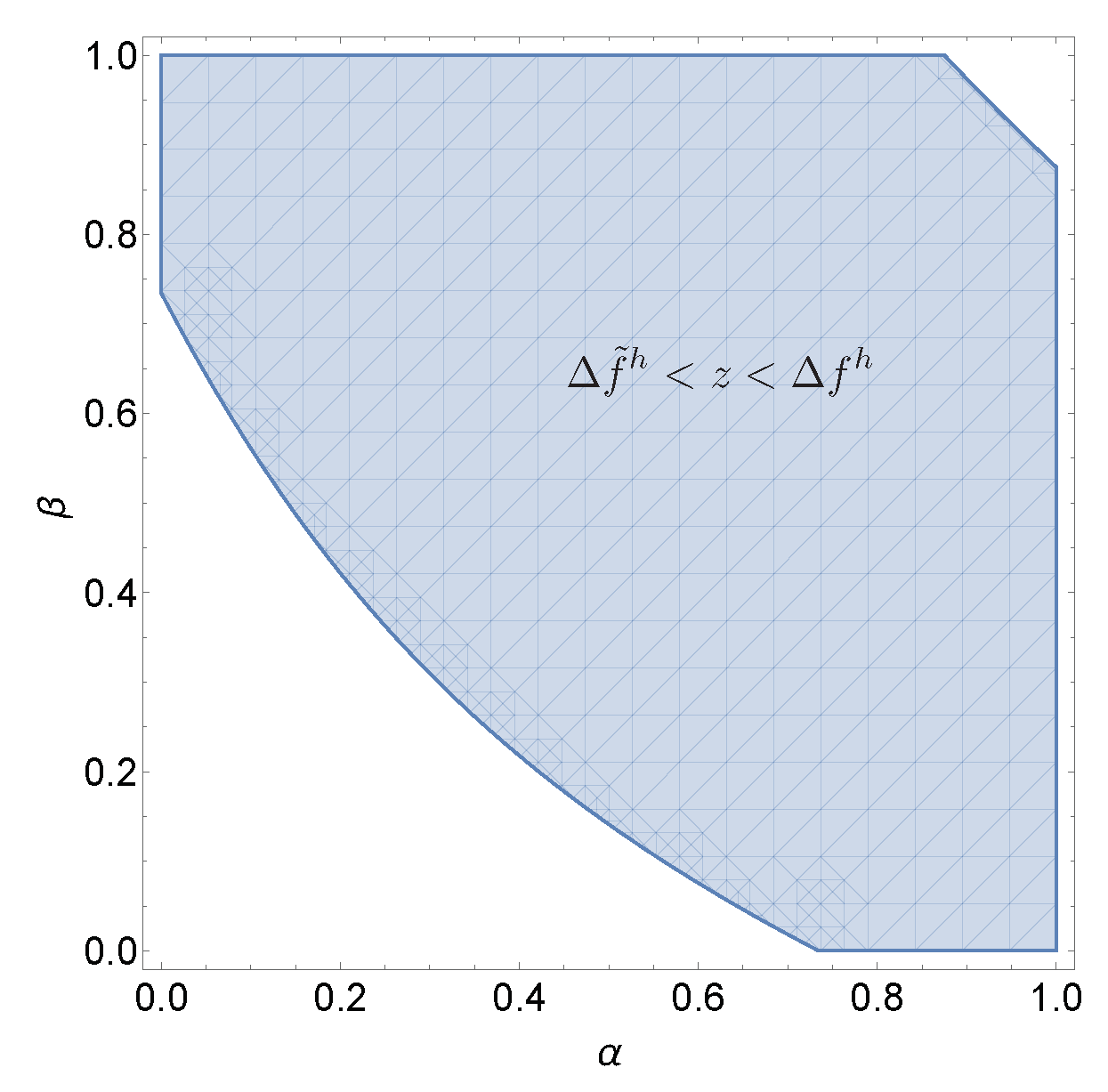
Result 2: When the status condition and the social comparison condition are fulfilled, there exists a range of parameters, and , so that the socially-optimal outcome is obtained with complete information about abilities, but not under incomplete information about abilities. This follows from the fact that for given parameters ( and ), . The effect of information about abilities is illustrated in Figure 3, where the solid lines are taken from Figure 2 and Figure 3. The shaded area between both lines represents combinations of and for which the socially-efficient outcome is obtained with complete information about abilities, but not under incomplete information about abilities. Formally, all points in the shaded area are combinations of and for which .
3. Discussion and Conclusions
Within this paper, we incorporated affective responses into a game-theoretical model, relaxing the unrealistic assumption about the irrelevance of emotions while maintaining the formal rigor of rational choice modeling. When models based on simple motivational assumptions (e.g., maximization of monetary gains) fail, a dual selves model, as the one presented in this paper, provides a sensible alternative.
By considering affective responses and the role of emotions, we analyzed a richer incentive scheme compared to material incentives. Our model showed that in order to achieve efficiency gains through the expression of esteem, information about abilities is crucial. With incomplete information about abilities, the socially-optimal outcome is achieved only when two conditions are fulfilled. Firstly, the expression of esteem has to be based on interpersonal comparisons. Secondly, the preference for esteem has to be a status preference.
In our model, we assumed complete information about preferences. That is, not only the material payoffs, but also the parameters that determine workers’ utility from esteem are common knowledge. This might be a realistic assumption when workers know each other very well, but in other situations, it might make more sense to assume incomplete information (see [15]). With incomplete information about esteem utility, a worker does not know the other worker’s strength of the status preference for esteem (), or the strength of the social comparison in expressing esteem (), or the amount of esteem received from other sources (k).
To see how our results would change if we assumed incomplete information about esteem utility would require a generalization of our model, which is beyond the scope of this paper. Since we believe that such an extension would be worthwhile, we provide a sketch of how one would proceed: For the sake of simplicity, we assume complete information about k, so that there is uncertainty only with respect to and . For each worker, a vector will be drawn from an exogenously-given distribution, and each pair of vectors will correspond to a state of nature. With such a framework, one could extend our model towards a psychological game with incomplete information.18
While the exposition of our model was focused on team production, there are overlaps with the literature on markets and organizations. Consider the distinction between transactions in markets and organizations, which is fundamental in institutional economics. Market interactions are typically ephemeral and anonymous; hence, it is unlikely that players know each others’ abilities. In many organizations, membership is stable; the same players interact repeatedly, and consequently, players know each other’s abilities. It follows that there is a wide range of parameters such that the expression of esteem will increase efficiency in organizations, but not in markets. Thus, our model provides an explanation for the existence of firms because only within organizations, players know each others’ abilities so that esteem incentives will increase efficiency. More specifically, information about workers’ abilities is a form of firm specific human capital, because it is information about specific people working in a specific team. When moving to a new firm, a worker’s information about the abilities of her/his old colleagues is worthless.
Our model has important implications for the design of organizations. Organizations should ensure that workers learn each other’s abilities because when others’ abilities are known, esteem incentives are more effective. Obviously, information about abilities is related to the organizations internal structure and turnover. For given turnover, efficiency could be increased by lowering the cost of learning about others’ abilities (e.g., shared offices instead of private offices). In organizations where turnover is low, it is likely that over time, workers learn about each others’ abilities, so that information about abilities is common knowledge.
The effectiveness of esteem incentives can be affected through several policies. Organizations should create opportunities that ensure the expression of esteem, for example, by creating a work environment in which there is enough room for the public expression of esteem through the exchange of esteem services, like paying attention, expressing opinions, or giving credit ([7], pp. 89–90). More precisely, esteem is provided unintentionally if a worker pays attention to her/his co-worker’s efforts. The decision to pay attention, however, is an intentional decision. Hence, workers are more likely to express esteem in organizations in which workers are interdependent and in organizations that create a cooperative work environment.
A very promising way for the expression of esteem is the use of symbolic awards, which are highly visible (e.g., [38]). Another possibility is peer evaluations, provided that the results are publicly available. Awards and peer evaluations are two possibilities for how workers can acknowledge their co-workers’ accomplishments publicly. Consequently, esteem will be expressed, and social approval can increase efficiency.
Funding
This research received no external funding.
Acknowledgments
Thanks to Max Albert, Klaus Wälde, and the two anonymous referees for constructive feedback.
Conflicts of Interest
The authors declare no conflict of interest.
Appendix A. Complete Information about Abilities
Figure A1 contains the extensive form representation of the game with complete information about abilities. The game starts at the black node in the middle, where nature moves and determines both workers’ types (= abilities). There are four subgames, one for each distribution of abilities. Denote these subgames by 1, 2, 3, and 4. Starting from the initial node, Subgame 1 moves upwards, Subgame 2 rightwards, Subgame 3 leftwards, and Subgame 4 downwards.
Nodes – are end nodes if stage three (the expression of esteem) is absent. The numbers at these nodes denote utilities derived from the payoffs resulting from team production and costs of effort. When Stage 3 is considered, the emotional selves simultaneously express esteem at nodes –.
Figure A1.
Game without esteem when abilities are public information. Dashed lines indicate information sets.
Figure A1.
Game without esteem when abilities are public information. Dashed lines indicate information sets.

In the four subgames, abilities are given by , , , and .
Let denote i’s utility in subgame q. Note that in the subgame, abilities are given; hence, each strategy profile for defines a pair of actions in this subgame. In the following, and .
Subgame 1: The subgame is not a proper game. Both workers have low abilities, so by assumption, . The utilities are:
Subgame 2: In Subgame 2, , but , so only Worker 2 can choose between high and low effort. The utilities are:
if Worker 2 chooses low effort and:
if he/she chooses high effort. Worker 2 chooses high effort, if:
Subgame 3: Subgame 3 is identical to Subgame 2, except that the roles are reversed. Hence, Worker 1 chooses high effort if Equation (A2) holds, and the equilibrium strategy profile is given by .
Subgame 4: In Subgame 4, the utilities are:
if both workers choose low effort,
if 1 chooses low effort and 2 chooses high effort,
if 2 chooses low effort and 1 chooses high effort, and
if both workers choose high effort.
Strategy profile is an equilibrium if:
and strategy profile is an equilibrium if:
If , profiles and are equilibria. Strategy profile is Pareto dominant since for .
Proof.
We have to show that
By assumption: , and f is increasing. It remains to show that , which holds true if because .
can be rewritten as:
which is true since both and are between zero and one. Q.E.D. □
Asymmetric equilibria: For the sake of completeness, we consider the asymmetric strategy profiles. The asymmetric strategy profiles and are equilibria if:
The asymmetric strategy profiles and are equilibria if and (for ), i.e.,
Appendix B. Incomplete Information about Abilities
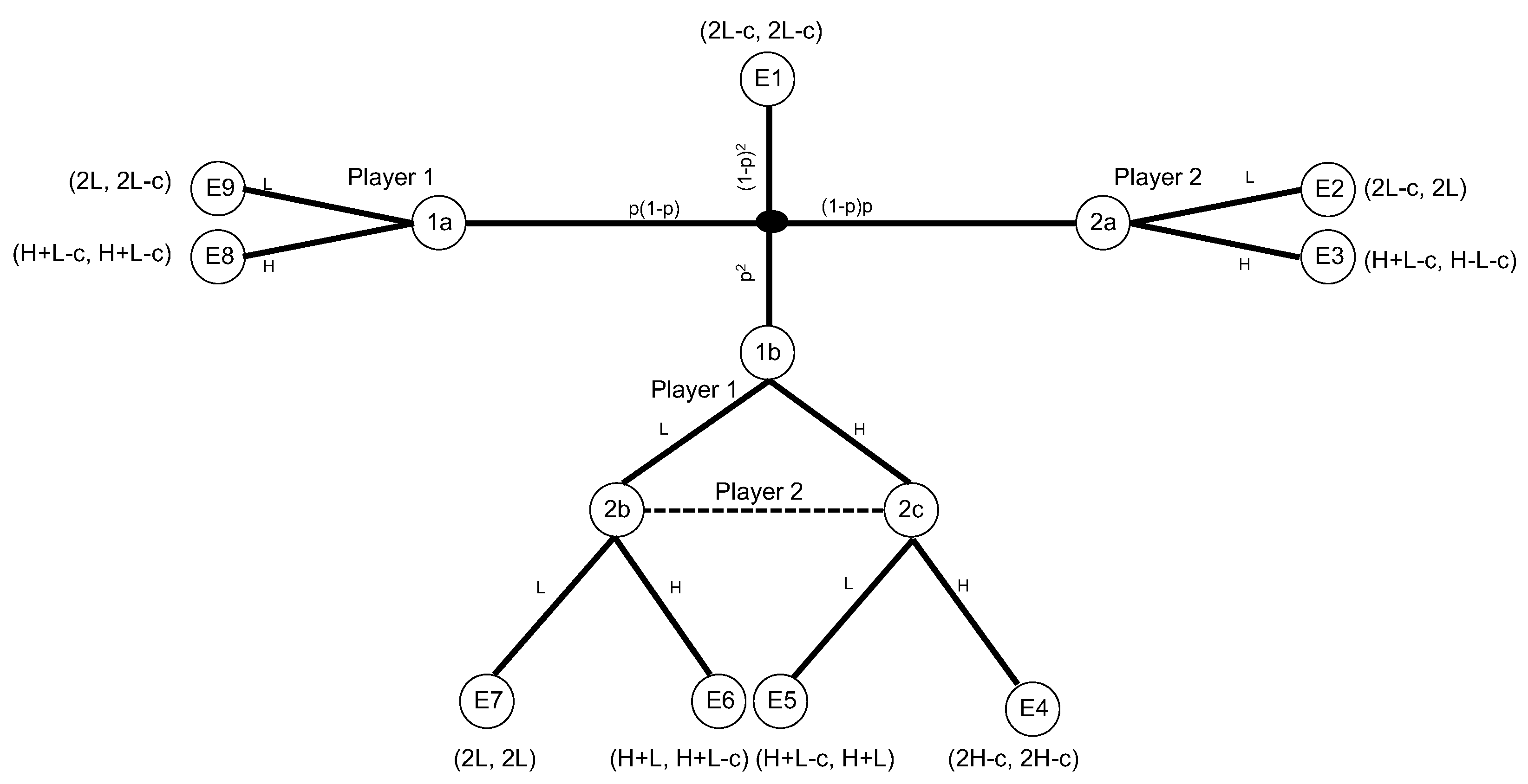
Figure A2 contains the extensive form representation of the game with incomplete information about abilities. The game starts at the black node in the middle, where nature moves and determines both workers’ types (= abilities). Each player only knows her/his own, but not the others’ type. At nodes and , Player 1 has high ability and chooses between high and low effort. At nodes , , and , Player 2 has high ability and chooses between high and low effort.
Nodes — are end nodes if Stage 3 (the expression of esteem) is absent. The numbers at these nodes denote utilities derived from the payoffs resulting from team production and costs of effort. When Stage 3 is considered, both emotional selves simultaneously express esteem at nodes —.
Figure A2.
Game without esteem when abilities are private information. Dashed lines indicate information sets.
Figure A2.
Game without esteem when abilities are private information. Dashed lines indicate information sets.

Table A1 depicts the nodes and information sets for the expression of esteem by Player 1’s emotional self, . Player knows her/his own ability (Line 1) and both effort levels ( and , Lines 2 and 3). In the pooling equilibrium, both workers choose low effort, so that effort choices do not signal abilities. In the following, we consider the pooling equilibrium.

Table A1.
Information of player in the game with esteem and incomplete information.
| L | L | L | H | H | H | H | H | H | |
| L | L | L | H | H | L | L | H | L | |
| L | L | H | H | L | H | L | L | L |
When expressing esteem, can distinguish six different information sets:
For the information sets that are not singletons, the corresponding beliefs are:
Assume that there are m different actions available for the expression of esteem, so that node is followed by nodes – (for ). Because both players ( and ) express esteem simultaneously, cannot distinguish between nodes –; they belong to the same information set.
Table A2 depicts the nodes and information sets for the expression of esteem by Player 2’s emotional self, . Player knows her/his own ability (Line 1) and both effort levels ( and , Lines 2 and 3).
Table A2.
Information of player in the game with esteem and incomplete information.
| to | to | to | to | to | |
| L | H | H | H | H | |
| L | L | L | H | H | |
| L | L | H | H | L | |
| to | to | to | to | ||
| H | H | L | L | ||
| L | L | H | L | ||
| H | L | L | L |
Based on information about his/her own ability and both workers choices of effort, can distinguish the following six different information sets:
Because the structure of the game is common knowledge, can compute ’s expression of esteem at each node. Let (for ) denote the nodes that follow ’s expression of esteem in equilibrium. All other nodes that follow ’s expression of esteem will never be reached (will be reached with probability zero). In the following, we look at the nodes that will be reached with positive probability. In total, there are nine nodes that will be reached with positive probability. can distinguish only between the following six information sets:
For the information sets that are not singletons, the corresponding beliefs are:
In the separating equilibrium, there is no uncertainty with respect to abilities because workers with low ability always choose low effort and workers with high ability always choose high effort.
References
- Battigalli, P.; Corrao, R.; Dufwenberg, M. Incorporating belief-dependent motivation in games. J. Econ. Behav. Org. forthcoming. [CrossRef]
- Caplin, A.; Leahy, J. Psychological expected utility theory and anticipatory feelings. Q. J. Econ. 2001, 116, 55–79. [Google Scholar] [CrossRef]
- Loewenstein, G. Emotions in Economic Theory and Economic Behavior. Am. Econ. Rev. 2000, 90, 426–432. [Google Scholar] [CrossRef] [Green Version]
- Loomes, G.; Sugden, R. Regret theory: An alternative theory of rational choice under uncertainty. Econ. J. 1982, 92, 805. [Google Scholar] [CrossRef]
- Gul, F. A Theory of Disappointment Aversion. Econometrica 1991, 59, 667. [Google Scholar] [CrossRef]
- Elster, J. Emotions and Economic Theory. J. Econ. Lit. 1998, 36, 47–74. [Google Scholar]
- Brennan, G.; Pettit, P. The Hidden Economy of Esteem. Econ. Philos. 2000, 16, 77–98. [Google Scholar] [CrossRef]
- Chaiken, S.; Trope, Y. Dual-Process Theories in Social Psychology; The Guilford Press: New York, NY, USA, 1999. [Google Scholar]
- Fudenberg, D.; Levine, D.K. A Dual-Self Model of Impulse Control. Am. Econ. Rev. 2006, 96, 1449–1476. [Google Scholar] [CrossRef] [Green Version]
- Evans, J.S.B.T. Dual-Processing Accounts of Reasoning, Judgment, and Social Cognition. Annu. Rev. Psychol. 2008, 59, 255–278. [Google Scholar] [CrossRef] [Green Version]
- Alós-Ferrer, C.; Strack, F. From dual processes to multiple selves: Implications for economic behavior. J. Econ. Psychol. 2014, 41, 1–11. [Google Scholar] [CrossRef]
- Sloman, S.A. The empirical case for two systems of reasoning. Psychol. Bull. 1996, 119, 3–22. [Google Scholar] [CrossRef]
- Frank, M.J.; Cohen, M.X.; Sanfey, A.G. Multiple Systems in Decision Making. Curr. Dir. Psychol. Sci. 2009, 18, 73–77. [Google Scholar] [CrossRef]
- Geanakoplos, J.; Pearce, D.; Stacchetti, E. Psychological games and sequential rationality. Games Econ. Behav. 1989, 1, 60–79. [Google Scholar] [CrossRef] [Green Version]
- Attanasi, G.; Nagel, R. A survey of psychological games: Theoretical findings and experimental evidence. In Games, Rationality and Behavior. Essays on Behavioral Game Theory and Experiments; Innocenti, A., Sbriglia, P., Eds.; Palgrave MacMillan: Basingstoke, UK, 2008; pp. 204–232. [Google Scholar]
- Battigalli, P.; Dufwenberg, M. Dynamic psychological games. J. Econ. Theory 2009, 144, 1–35. [Google Scholar] [CrossRef]
- Attanasi, G.; Battigalli, P.; Manzoni, E.; Nagel, R. Belief-dependent preferences and reputation: Experimental analysis of a repeated trust game. J. Econ. Behav. Org. forthcoming. [CrossRef]
- Charness, G.; Dufwenberg, M. Promises and Partnership. Econometrica 2006, 74, 1579–1601. [Google Scholar] [CrossRef]
- Dufwenberg, M.; Gächter, S.; Hennig-Schmidt, H. The framing of games and the psychology of play. Games Econ. Behav. 2011, 73, 459–478. [Google Scholar] [CrossRef] [Green Version]
- Attanasi, G.; Battigalli, P.; Manzoni, E. Incomplete-information models of guilt aversion in the trust game. Manag. Sci. 2015, 62, 648–667. [Google Scholar] [CrossRef]
- Dufwenberg, M.; Dufwenberg, M.A. Lies in disguise–A theoretical analysis of cheating. J. Econ. Theory 2018, 175, 248–264. [Google Scholar] [CrossRef]
- Holländer, H. A Social Exchange Approach to Voluntary Cooperation. Am. Econ. Rev. 1990, 80, 1157–1167. [Google Scholar]
- Kandel, E.; Lazear, E.P. Peer Pressure and Partnerships. J. Political Econ. 1992, 100, 801–817. [Google Scholar] [CrossRef]
- Mas, A.; Moretti, E. Peers at Work. Am. Econ. Rev. 2009, 99, 112–145. [Google Scholar] [CrossRef]
- Itoh, H. Moral Hazard and Other-Regarding Preferences. Jpn. Econ. Rev. 2004, 55, 18–45. [Google Scholar] [CrossRef]
- Rey-Biel, P. Inequity Aversion and Team Incentives. Scand. J. Econ. 2008, 110, 297–320. [Google Scholar] [CrossRef]
- Demougin, D.; Fluet, C. Group vs. individual performance pay when workers are envious. In Contributions to Entrepreneurship and Economics; Demougin, D., Schade, C., Eds.; Duncker and Humblot Verlag: Berlin, Germany, 2006; pp. 39–47. [Google Scholar]
- De Marco, G.; Immordino, G. Reciprocity in the Principal–Multiple Agent Model. BE J. Theor. Econ. 2014, 14, 445–482. [Google Scholar] [CrossRef]
- Fehr, E.; Gächter, S. Cooperation and Punishment in Public Goods Experiments. Am. Econ. Rev. 2000, 90, 980–994. [Google Scholar] [CrossRef]
- Belot, M.; Van de Ven, J. How private is private information? The ability to spot deception in an economic game. Exp. Econ. 2016, 20, 19–43. [Google Scholar] [CrossRef] [Green Version]
- Postlewaite, A. The social basis of interdependent preferences. Eur. Econ. Rev. 1998, 42, 779–800. [Google Scholar] [CrossRef]
- Rabin, M. Incorporating Fairness Into Game Theory and Economics. Am. Econ. Rev. 1993, 83, 1281–1302. [Google Scholar]
- Crawford, V.P.; Sobel, J. Strategic Information Transmission. Econometrica 1982, 50, 1431. [Google Scholar] [CrossRef]
- Bénabou, R.; Tirole, J. Mindful Economics: The Production, Consumption, and Value of Beliefs. J. Econ. Perspect. 2016, 30, 141–164. [Google Scholar] [CrossRef] [Green Version]
- Epley, N.; Gilovich, T. The Mechanics of Motivated Reasoning. J. Econ. Perspect. 2016, 30, 133–140. [Google Scholar] [CrossRef]
- Bracha, A.; Brown, D.J. Affective decision making: A theory of optimism bias. Games Econ. Behav. 2012, 75, 67–80. [Google Scholar] [CrossRef] [Green Version]
- Battigalli, P.; Dufwenberg, M. Guilt in games. Am. Econ. Rev. 2007, 97, 170–176. [Google Scholar] [CrossRef]
- Kosfeld, M.; Neckermann, S. Getting More Work for Nothing? Symbolic Awards and Worker Performance. Am. Econ. J. Microecon. 2010, 3, 86–99. [Google Scholar] [CrossRef]
| 1 | Emotions can be categorized with regard to the time at which they are experienced. Expected or anticipatory emotions are experienced before the outcome occurs [1]. In Caplin and Leahy [2], for example, investors experienced anxiety before uncertainty about future states is resolved. An example for an immediate emotion is hunger, which affects an individual’s preference for food during consumption [3]. Lastly, there are expected emotions, which are expected to be experienced as a result of an outcome. Expected emotions have been discussed, for example, in the literature on regret and disappointment aversion [4,5]. |
| 2 | Other physiological expressions of emotions, which are beyond rational choice, are voice pitch, flushing and blushing, smiling, laughing, and crying. |
| 3 | The work in [20] represented an extension of psychological game theory to incomplete information models, which we will discuss in Section 3. The work in [21] emphasized the role of beliefs at end nodes. Two further related models were given by [22,23]. However, these models did not explicitly model the belief-dependence of emotions and utilities; hence, we do not discuss them in more detail. |
| 4 | Two examples are surprise and respect. Both emotions depend on players’ information, which is updated as the game unfolds. |
| 5 | This could be interpreted either as low types always choosing low effort because higher choices of effort would not increase individual productivity or because the cost of choosing a higher level of effort is enormously high. |
| 6 | |
| 7 | An anonymous referee suggested that negative feelings are more likely to be expressed publicly. Of course, one could rewrite the model with anger instead of esteem. We believe that this would not affect the results because “expressing esteem towards work X” would be equivalent to “not being angry about worker X”. |
| 8 | Since workers have a status preference for esteem, as described in the next section, expressing esteem affects a worker’s utility indirectly. |
| 9 | Elster [6] (p. 67) made a similar point and argued that norm violators are sanctioned even if punishment is costly for the sanctioner. A large number of experiments on punishment in public goods games (e.g., [29]) and the ultimatum and power-to-take game confirms this argument. Lastly, there is experimental evidence that people are able to spot deception in face-to-face communication, suggesting that “fake” emotions will be recognized as being “fake” (see [30] and the references cited therein). |
| 10 | Our modeling strategy belongs to what Postlewaite [31] calls the “direct” approach because a player’s concern for status is an argument in the utility function. The “direct” approach is in contrast with the “instrumental” approach, according to which status is valued only indirectly because higher status provides better access to other resources. Based on evolutionary arguments, Postlewaite [31] argued in favor of the “direct” approach. |
| 11 | One can think of k as esteem received from others, but it can also depend on a worker’s characteristics, such as her/his self-confidence. Using a positive parameter k can be seen as a normalization so that , which is necessary, for example, if . |
| 12 | Although the existence of two social comparisons might seem a bit redundant at this point, the reason for having both comparisons will hopefully come clear when we discuss the model’s equilibria. As we will see, with complete information about abilities, an equilibrium in which both workers choose high effort can be attained if or is high. With incomplete information about abilities, such an equilibrium will only exist if both and are high enough. |
| 13 | This case is similar to Example 2 in Rabin [32]. |
| 14 | At this point, we would like to stress the flexibility of our model. The assumption that the emotional self uses Bayesian updating to compute conditional expectations might seem unrealistic, given the empirical literature on belief formation. An emotional self, whose preferences are defined by the negative quadratic loss function, represents the extreme case in which the emotional self is motivated only by the accuracy of information. Obviously, it would be possible to derive the affective response from another utility function that includes other motivational factors or cognitive biases, like conservatism in belief-updating, motivated reasoning, or optimism bias (see [34,35,36]). |
| 15 | Formally, we now have a game consisting of four players, two workers where each worker consists of a rational and an emotional self. Each rational self’s strategy set is ; each emotional self’s strategy set is the interval 0–1. Rational selves simultaneously choose efforts before emotional selves simultaneously choose conditional expectations. Payoffs are given by Equation (2) for rational selves and the quadratic loss function for emotional selves. |
| 16 | For the sake of completeness, we specify the nodes at which esteem is expressed and the corresponding beliefs in Appendix B. |
| 17 | holds only if f is extremely curved and both and are close to one. Then, there is a unique equilibrium in pure strategies for high and for low values of z. For intermediate values of z, there are two equilibria in pure strategies. |
| 18 | We guess that our results are robust if workers’ ()-values are drawn from the same distribution and if this distribution is known, because workers’ beliefs would be identical. The results might change if the distribution is not known to workers because, then there will be heterogeneity in beliefs. For example, this would be the case if one worker knows that she/he is more sensitive to social comparisons than her/his co-worker. For a full-blown analysis of such a model, see [20]. |
Figure 1.
Equilibria with complete information about abilities. Figure 1 shows equilibria as a function of and when abilities are common knowledge. In Region (1), workers always choose high effort; in Region (3), they always choose low effort; and in Region (2), two pure strategy equilibria exist. The parameters used in Figure 1 are , , , , and .

Figure 2.
Equilibria with incomplete information about abilities. Figure 2 shows equilibria as a function of and with incomplete information about abilities. In Region (1), workers always choose high effort (separating equilibrium); in Region (3), they always choose low effort (pooling equilibrium); and in Region (2), there exists no equilibrium in pure strategies. The parameters used in Figure 2 are , , , , and .

Figure 3.
Socially-optimal outcome with complete information about abilities, but not with incomplete information. Figure 3 depicts the effect of information about abilities. The shaded area between both curves represents combinations of and for which the socially-efficient outcome is obtained if abilities are common knowledge, but not if abilities are private information. The parameters used in Figure 2 are , , , , and .

© 2019 by the author. Licensee MDPI, Basel, Switzerland. This article is an open access article distributed under the terms and conditions of the Creative Commons Attribution (CC BY) license (http://creativecommons.org/licenses/by/4.0/).
Share and Cite
MDPI and ACS Style
Greiff, M. Team Production and Esteem: A Dual Selves Model with Belief-Dependent Preferences. Games 2019, 10, 33. https://0-doi-org.brum.beds.ac.uk/10.3390/g10030033
AMA Style
Greiff M. Team Production and Esteem: A Dual Selves Model with Belief-Dependent Preferences. Games. 2019; 10(3):33. https://0-doi-org.brum.beds.ac.uk/10.3390/g10030033
Chicago/Turabian StyleGreiff, Matthias. 2019. "Team Production and Esteem: A Dual Selves Model with Belief-Dependent Preferences" Games 10, no. 3: 33. https://0-doi-org.brum.beds.ac.uk/10.3390/g10030033
Note that from the first issue of 2016, this journal uses article numbers instead of page numbers. See further details here.