Generalized Backward Induction: Justification for a Folk Algorithm


Department of Political Science and Mathematical Behavioral Sciences, University of California, 3151 Social Science Plaza, Irvine, CA 92697-5100, USA
Games 2019, 10(3), 34; https://0-doi-org.brum.beds.ac.uk/10.3390/g10030034
Submission received: 11 June 2019
/
Revised: 12 August 2019
/
Accepted: 27 August 2019
/
Published: 30 August 2019
(This article belongs to the Special Issue Political Economy, Social Choice and Game Theory)
Abstract
:I introduce axiomatically infinite sequential games that extend Kuhn’s classical framework. Infinite games allow for (a) imperfect information, (b) an infinite horizon, and (c) infinite action sets. A generalized backward induction (GBI) procedure is defined for all such games over the roots of subgames. A strategy profile that survives backward pruning is called a backward induction solution (BIS). The main result of this paper finds that, similar to finite games of perfect information, the sets of BIS and subgame perfect equilibria (SPE) coincide for both pure strategies and for behavioral strategies that satisfy the conditions of finite support and finite crossing. Additionally, I discuss five examples of well-known games and political economy models that can be solved with GBI but not classic backward induction (BI). The contributions of this paper include (a) the axiomatization of a class of infinite games, (b) the extension of backward induction to infinite games, and (c) the proof that BIS and SPEs are identical for infinite games.
Keywords:
subgame perfect equilibrium; backward induction; refinement; axiomatic game theory; agenda setter; imperfect information; political economyJEL Classification:
C731. Introduction
The origins of backward induction are murky. Zermelo [1] analyzed winning in chess, asking a question about the winning strategy for white in a limited number of moves, yet his method of analysis was based on a different principle [2]. A couple of decades later, we find that reasoning based on backward induction was implicit in Stackelberg’s [3] construction of his alternative to the Cournot equilibrium. Then, as a general procedure for solving two-person, zero-sum games of perfect information, backward induction appeared in von Neumann and Morgenstern’s [4] (p. 117) founding book, which followed von Neumann’s [5] earlier question about optimal strategies. BI was also used to prove a precursor of Kuhn’s Theorem for chess and similar games. Von Neumann’s exceedingly complex formulation was later clarified and elevated to high theoretical status by Kuhn’s [6] work, most especially, Corollary 1; Schelling’s [7] ideas about incredible threats; and Selten’s [8] introduction of subgame perfection. However, it suffered drawbacks when the chain-store paradox, Centipede, and other games brought into doubt its universal appeal [9,10]. Its profile was further lowered with new refinements: perfect equilibrium [11], sequential equilibrium [12], and particular procedures such as forward induction [13] offered solutions that often seemed more intuitive. The arguments against applying backward induction began to multiply, sealing doubts about its universal validity [14,15,16,17,18,19,20,21,22].
The goal of the present paper is to extend backward induction to infinite games with imperfect information and to investigate its relation to subgame perfection. In its standard formulation, backward induction applies only to finite games of perfect information. In these cases, every backward induction solution (BIS), i.e., a strategy profile that survives backward “pruning” (a subsequent substitution of terminal subgames with Nash-equilibrium payoffs), is also a subgame perfect equilibrium (SPE) and all SPEs result from backward pruning [23] yet it is common knowledge among game theorists that other games can be solved through backward reasoning as well; they have routinely applied the procedure to such games for half a century. Backward reasoning is implicit in refining the Stackelberg equilibrium from other Nash equilibria (NE). Schelling analyzed backward the NE in the iterated Prisoner’s Dilemma as early as in the 1950s [24]. Reputable textbooks, such as those by Fudenberg and Tirole [25] (p. 72) and Myerson [26] (p. 192), make explicit claims—although without proofs—that backward induction can be applied to a wider class of games. Osborne and Rubinstein [27] (p. 98, Lemma 98.2 on one deviation property) essentially extend backward induction to finite-horizon extensive games with perfect information. Additionally, Escardó and Oliva [28] showed that BIS is equivalent to SPE in certain well-founded games, i.e., games with perfect information, such that all paths must be finite, even though they may be arbitrarily long. Moreover, backward reasoning is commonly applied to solve various parametrized families of extensive-form games in political economy models. It is also used implicitly when one argues that voters “vote sincerely ” in the last stage of various voting games that have binary agendas.
What results from this alleged abuse? Perhaps most clearly, Fudenberg and Tirole [25] (p. 94) spell out the underlying principle: “This is the logic of subgame perfection: Replace any ’proper subgame’ of the tree with one of its Nash-equilibrium payoffs, and perform backward induction on the reduced tree.” With caveats discussed later in this introduction, Fudenberg and Tirole’s prescription captures the essence of the generalized backward induction (GBI) approach. However, if one wanted to find an entirely formal (i.e., axiomatic) justification for this algorithm in the literature, one would not be able to do so, yet such a justification is necessary since, in fact, the principles behind SPE and BIS differ.
We can informally examine this petite difference. SPE is a strategy profile that is NE in all subgames. Its intuitive justification focuses on subgames, i.e., smaller games within a larger one. SPE demands that players interact “rationally” in all subgames, i.e., that they apply strategies resulting in NE in the subgames. Unless a game has no other subgames than itself, backward induction concerns different games. It starts at the game’s end and moves backward. Similar to SPE, the first game (or a set of games) is a subgame. However, at some point, a new game appears that is not a subgame of the original game and which has no counterpart in the SPE’s definition. Such a game (or games) is created by substituting a subgame (or subgames) with an NE payoff vector in those subgames.
A simple example illustrates the distinction. In Figure 1, SPE in game G requires that Bob and Alice play NE strategies in both the original game G and its subgame H. BIS requires that the players play NE strategies in G’s subgame H and also the “upgame” J. J was created by “pruning” H, i.e., substituting the root of H with an endnode that had the NE payoffs in H assigned as payoffs.
Backward induction is helpful because the games that we need to solve when using its algorithm are usually smaller and simpler than those that appear in the definition of the SPE. It seems such an obvious route toward finding SPEs that one can easily ignore the subtle difference in the definitions, especially when one begins to struggle with the truly painful chore of defining BIS formally. Nevertheless, one cannot state a priori that the sets of strategy profiles obtained in both cases are identical.
Despite the lack of a firm foundation, it seems that, within the discipline, backward induction has acquired the status of a “folk algorithm”Ȧlthough game theorists use it, it appears that little attention has been paid to its rigorous examination. It clearly works—in the sense that it produces SPEs—but we neither know exactly for what games it works nor precisely what it produces. The formal link between the folk algorithm and subgame perfection remains obscure.
In the current paper, I investigate the “folk puzzle of backward induction” axiomatically. The axiomatic framework that I introduce below encompasses more games than the finite games axiomatized by either von Neumann and Morgenstern [4] or Kuhn [6]. Specifically, in this work, the action sets may be infinite (more formally, they can have any cardinality) and the length of a game may be infinite (denumerable). Despite its higher complexity, this new framework allows for a constructive analysis.
The results of this work certify that, with some clarification, the folk wisdom linking BI and SPE is correct for various sets of infinite games. Nevertheless, it is also clear that Fudenberg and Tirole’s [25] prescription of applying BI over subgames has to be modified. The informal description of these modifications is as follows:
First, backward pruning can be applied not only to pure strategies but also to certain behavioral strategies.
Second, we must replace every subgame with an SPE and not an NE payoff vector. Obviously, when a subgame has no other subgames than itself, SPE and NE coincide.
Finally, we can replace entire subsets of disjoint subgames simultaneously, not only single subgames. Such simultaneous replacement is essential not only for solving many games that are not finite but also for certain complex finite games, as it may be the only realistic way to proceed (see Example 1).
Remarkably, in agreement with the case of finite games of perfect information, the findings show that, for pure strategies and certain behavioral strategies, the sets of BIS and SPE coincide. This is the main result of the present work. It legitimizes the informal methods of backward pruning of a game, and it concatenates the resulting partial strategy profiles used by game theorists to solve games.
The generalized algorithm uses the agenda—the tree consisting of the roots of all subgames—instead of the game tree. For games of perfect information, the agenda coincides with the game tree with terminal nodes subtracted. A step in such an algorithm can informally be compared to the classic backward induction as follows:
- (1)
- Prune (remove) any subset of disjoint subgames instead of a single subgame, which would have only one decision node followed by terminal nodes.
- (2)
- Substitute all selected subgames with the SPE payoffs instead of the payoffs for best moves.
- (3)
- Concatenate all partial strategy profiles obtained in the previous step; if at any point one gets an empty set, this would mean that there is no SPE in the game.
The above three-step procedure can be applied to pure strategies in all games as well as to behavioral strategies that satisfy the condition of finite support and crossing. Finding all SPEs requires following particular rules for concatenating and discarding partial strategy profiles, as described in Section 4 of this paper.
The next section introduces axiomatically sequential games with potentially infinite sets of actions and an infinite horizon. While a more accurate label would be “potentially infinite ” here, I call such games “infinite” for the sake of simplicity. Following the introduction of these games, I establish the basic facts linking payoffs to strategies in infinite games. Then, in Section 3, I investigate the decomposition of games into subgames and upgames for pure and behavioral strategies with finite support and crossing. The reader who is more interested in applications may skip Section 2 and Section 3 and go directly to Section 4, where the GBI algorithm is formally described. Then, in the subsequent section, I discuss five illustrative examples, including the application of the procedure to solve parametrized games, which are often used in political economy modeling and an ad hoc generalization that finds the unique perfect equilibrium. Finally, I conclude the paper in Section 6 with the remaining open questions as well as suggestions for further research. All proofs are found in the Appendix A.
2. Preliminaries
Sequential (extensive-form) games were introduced with a set-theoretic axiomatization by von Neumann and Morgenstern [4] (pp. 73–76). They were conceived and presented in the spirit of the rigorous decoupling of syntax and semantics in the early 20th century, such as embodied in the works of Hilbert and Tarski and, later, in Bourbaki’s team. In order to prevent a reader from forming any geometric or other intuition, von Neumann [4] proudly announced that “we have even avoided giving names to the mathematical concepts […] in order to establish no correlation with any meaning which the verbal associations of names may suggest” (p. 74). Then, he dismissed his own idea of a game tree, as “even relatively simple games lead to complicated and confusing diagrams, and so the usual advantages of graphical representation do not obtain” (p. 77). Despite von Neumann’s every effort to turn a sequential game into a highly abstract object, incomprehensible for nonmathematicians, Kuhn’s [6] approach helped to make games more intuitive. Kuhn simplified von Neumann’s formalism and built the axioms into definitions and assumptions about the tree, the players, and the information, as well as slightly generalized von Neumann’s unnecessarily narrow definition.
The axiomatic setup of the current paper goes beyond finite games in an attempt to cover axiomatically a larger class of extensive-form games. As mentioned above, for simplicity, such games are called infinite games. The framework maintains the compatibility with Kuhn’s pragmatic exposition and draws from the excellent modern presentations of finite games by Myerson [26] and Selten [11]. The axioms are divided into two subsets. The properties defining an infinite tree are listed explicitly; the game axioms are combined with the description of the game components and specify how various objects are attached to the tree. In order to establish some intuitive associations, I place in parentheses the axioms’ names that succinctly describe their content.
The way in which games are introduced is laborious, but it helps later with the succinct establishment of the basic results.
Rooted tree: Let be such that T is a set of at least two points, is a binary relation over T, and For a path to y of length k is any finite indexed set such that and for all , ; for For the path to is . For an infinite indexed set, is an infinite path if for every is a finite path.
is termed a rooted tree with its root and the set of nodes T if the following properties (AT1-AT3) are satisfied:
- AT1 (partial anti-reflexivity): For all iff ;
- AT2 (symmetry): For all iff ;
- AT3 (unique path): For every , there is exactly one path to x.
The following definitions and notation are used hereafter (the definitions are slightly redundant):
1. Binary relations between two different nodes :
Predecessor: (precedes x or is in the path to x) iff ;
Successor: (follows x) iff ;
Immediate predecessor: (immediately precedes x) iff
By AT1-AT3, for every , there is exactly one immediate predecessor.
Immediate successor: (immediately follows) x iff ;
Immediate predecessor in: For , (immediately precedes x in ) iff and .
By AT1-AT3, for every x and , there is at most one immediate predecessor of x in . This definition allows us to import the relation of preceding from the game tree into a smaller tree consisting of the roots of the game’s subgames (i.e., the game’s agenda). GBI will be conducted over the agenda.
2. Single nodes, subsets of nodes, set of subsets of nodes
Endnode (terminal node): a node x that is not followed by any other node, i.e., ;
Set of all endnodes: ;
Decision node: a node that is not an endnode;
Set of all decision nodes: ;
Branch: any node except for the root . (In a standard definition, a branch is any element (. For the simplicity of forthcoming notation, it is identified here with the node in the pair that is farther from the root.)
Alternative (originating) at a node x: any immediate successor of x;
Terminal path: a path to an endnode or an infinite path;
Set of all terminal paths .
Definition 1.
Game: An n-player sequential game is a septuple that includes a rooted game tree Ψ and the following objects: players from with their assigned decision nodes and probability distributions for random moves ; the pattern of information I; the identification of moves A; the probability distributions over random (or pseudorandom) moves h; and the payoff function P.
The conditions imposed on the components of G and certain useful derived concepts are defined below.
- Game tree: is a rooted tree with a set of nodes T, a set of decision nodes , a set of endnodes , and the root ;
- Players: For a positive integer n, consists of players and nature—a random or pseudorandom mechanism, labeled with 0;
- Player partition: is the partition of into (possibly empty) subses and a (possibly empty) subset for nature. The following assumptions are made regarding :
- (i)
- There is no path that includes an infinite number of nodes from ; 1‘
- (ii)
- For every , the number of alternatives at x is greater or equal two and finite.
- Information: is such that every is a partition of i’s set . We assume the following:
- (i)
- All elements of are singletons;
- (ii)
- For all , every element of includes only nodes with equal numbers (or cardinalities) of alternatives and does not include two nodes that are in the same path;
- (iii)
- (Perfect Recall): If is a successor of and is in the same information set with , then and must be immediate successors of either or some other node that is a successor of .For every , a set is called i’s information set. A node y originates from the information set if y originates at a node .
- Moves (actions): is a collection of partitions, one for every information set of every player i, of all alternatives originating at , such that for any node , every member of includes exactly one alternative that originates at x. The elements are called the moves (or actions) of i at For any , the moves at are singletons, including branches originating at . By definition, since every branch y belongs to precisely one move, for the move a such that is denoted by .
- Random moves: h is a function that assigns to every information set of the random mechanism a probability distribution over the alternatives at x, with all probabilities being positive. If h is not defined.
- Payoffs (associated with terminal paths): The payoff function assigns to every terminal path a payoff vector at e equal to . The component is called the payoff of player i at e. Function is called the payoff function of player i.
Both infinite paths and infinite numbers of moves at the players’ information sets are allowed. The assumed constraints demand that the numbers of players, the random information sets at every path, and the random moves at every random information set are finite. Another restriction is the discrete temporal structure of moves implied by the definition of game tree. Such a restriction excludes differential games and, in general, games in continuous time. Finally, games like stochastic games are conceptualized differently than extensive-form games (see, e.g., Reference [29]. Hereafter, the word “game” refers to Definition 1.
The most extensively studied subset of infinite games are finite games:
Finite game: G is finite if its set of nodes T is finite.
The concepts that follow are derived from the model’s primitives.
Subgame: For any game a subgame of G is any game , such that
- (i)
- is a subtree of , i.e., for some , or and ;
- (ii)
- If for some in G, then either or (either both and are in or neither is);
- (iii)
- The sets of players are identical () and are restrictions of P to , respectively.
It is straightforward that restrictions in (iii) define a game and that “being a subgame” is a transitive relation.
A player i may be a dummy in a game, i.e., may be empty. Since , the root of is a decision node and there must be at least one player or random mechanism in the game. Without loss of generality, one can assume that there are no dummies in the initial game G for which all results are formulated.
Below, the strategies are defined in order to optimize the introduction of the fundamental ideas—for this paper—of strategy concatenation and decomposition. The adjective “behavioral” is optional since behavioral strategies are our departure point for defining other types of strategies.
Behavioral actions: A behavioral action of finite support (in short, a behavioral action) of player i at the information set is a finite probability distribution over the set of actions .
A behavioral action at any information set assigns positive probabilities only to a finite number of actions at this set. When I refer to “finite support,” I will also mean the assumption in the definition of a game that the number of random actions is also finite.
Strategies (rough behavioral): A rough behavioral strategy of player i is any (possibly empty) set of i’s behavioral actions that includes exactly one behavioral action per information set of i. A partial rough behavioral strategy is any subset of a rough strategy. A partial rough strategy that includes exactly those actions in that are defined for information sets of i in a subgame H of G is denoted as and is called reduced to H.
The possibility of having an empty set of i’s behavioral actions represents a trivial strategy of player i in a subgame where i makes no moves. A rough behavioral strategy may be assembled from any set of actions. Below, this option is restricted to rough strategies that satisfy finite crossing.
For any rough strategy , we denote the probability assigned by at to a move by . A path e is called relevant for if chooses every alternative in e that originates from some information set of i with a positive probability, i.e., if for every node such that for some , . Finally, a path e crosses if .
Finite crossing in subgames: For every , a rough strategy is said to satisfy finite crossing in the subgames if for every subgame H of G and every path in H that is relevant for reduced to H, , crosses only a finite number of information sets from , such that the distribution is nondegenerate, i.e., it assigns positive probabilities to at least two actions.
Behavioral strategy: For any , a behavioral strategy of i—or simply, a strategy of i—is any rough strategy of i that satisfies finite crossing in subgames.
Comment: Finite support and finite crossing guarantee that, in all subgames, the payoffs (to be defined later) for behavioral strategies can be derived from a finite probability distribution. The class of strategies that satisfy these conditions includes, among others, all behavioral strategies in a finite game and all pure strategies in any game. Relaxing these conditions would introduce complications of a measure-theoretic nature along the lines examined by Aumann [30]. It is unclear whether the results would survive a more general treatment of behavioral strategies.
All behavioral strategies of i form i’s behavioral strategy space . Elements of are called behavioral strategy profiles and are denoted by .
I use a set-theoretic interpretation of strategies that will greatly simplify the definitions of strategy decomposition and concatenation as well as the treatment of partial strategy profiles. There is a simple isomorphism between strategy profiles defined in a set-theoretic and standard way. Thus, every strategy profile is interpreted as a union of players’ strategies (which are obviously disjoint); the Cartesian product is interpreted as taking all possible unions of individual strategies, one per player; the notation for the strategy profile represents an alternative notation for One example of the notational difficulty that is avoided is the interpretation of when at least one strategy set is empty. Another example is provided by the next definition.
A strategy profile with the strategy of player i removed, i.e., , is denoted by ; denotes with substituted with , that is, .
When such a distinction is necessary, the payoff functions, strategies, strategy profiles, etc. in games or in subgames G and H will be given the identifying superscripts , , etc.
The most important step toward building the framework for infinite games is expressing payoffs in terms of strategies.
Recall that the probability assigned by at to a move was denoted by . For any —such that and —and , the probability of the move to x is defined as . By convention, for all A path e is included in if for all , and it is denoted as . The set of all terminal paths included in is denoted by . The probability of playing e under , , is defined as follows:
Thus, is the product of the probabilities assigned by to all alternatives in e. Note that by the definition of the game and the behavioral strategy’s finite support of crossing, for a path of infinite length, only a finite number of alternatives may be assigned probabilities different than zero or one. The multiplication over an infinite series of numbers has at least one zero equal to zero, and an infinite product of ones is equal to one.
The probability of reaching a node y, , is defined as the probability of playing under :
The assumptions of finite support and finite crossing are used below to establish the fundamental fact that defines a probability distribution over a finite subset of all terminal paths.
Lemma 1.
For every game G and every subgame H of G and with the behavioral strategy profile ,
- (a)
- the set of all terminal paths in H included in , , is non-empty and finite;
- (b)
- for every , iff ;
- (c)
- .
Lemma 1 establishes that the probability distributions associated with actions of every behavioral strategy in a profile define a finite probability distribution on the set of all terminal paths. This allows us to extend the definition of the payoffs that were originally defined only for terminal paths to all behavioral strategy profiles of finite support and finite crossing.
Payoffs (for behavioral strategy profiles): For every behavioral strategy profile , for .
In the spirit of conserving letters, the original letter P that denotes payoffs assigned to the terminal paths is recycled here.
Finally, pure strategies are defined as a special case of behavioral strategies.
Pure strategies:, such that is always degenerate, i.e., picks only one action with certainty, is called a pure strategy and is denoted by . For pure strategies, the notation is used in place of and is used in place of B.
Decomposition of strategies: The definitions offered below introduce certain partial strategies or strategy profiles for G and :
- is reduced to H if ;
- is a complement of with respect to H if ;
- is a complement of with respect to
- is the set of all for all ;
- .
Let denote the decomposition function for player i, which assigns to its reduced strategy and its complement . The decomposition function is defined as . The following simple but useful result holds for every game G and its subgame H:
Lemma 2.
(a) For every i, is 1-1 and onto;
(b) is 1-1 and onto.
Lemma 2 allows us to define the function of the concatenation of strategies that is the inverse of decomposition: For every subgame H of G and every pair of partial strategy profiles and , is such that . Moreover, , where every is the inverse of a respective . Similar to , both and all its all components are 1-1 and onto.
The final two definitions of this section introduce two familiar equilibrium concepts [8,31]. For any game G and the strategy profile , the equilibrium conditions for are stated as follows:
- Nash equilibrium (NE): For every , ;
- Subgame perfect equilibrium (SPE): For every subgame H, is an NE in H.
Analogous definitions hold when all considered strategies are pure.
3. Decomposition of Strategies
The notations , , , etc. are used to denote the strategies, strategy profiles, strategy spaces, joint strategy spaces, etc. that are either pure or behavioral in order to process both cases simultaneously. Lemma 2 guarantees that the operations and are well defined and that they bring unique outcomes within the same family of strategies. Obviously, the family of pure strategies has the same property. Moreover, the definition of finite support of every strategy guarantees that the outcomes of and have finite support.
The profiles or denote any strategy profiles in G, and (or ) denote their decomposition with respect to its subgame H.
The sets and denote all terminal paths from that do not include the root of H, , or that do include , respectively:
- such that ;
- such that .
Lemma 3 states that the payoff in any game G from any strategy profile is the sum of the payoffs from all terminal paths that do not include and the payoff of reduced to H multiplied by the probability of reaching .
Lemma 3.
.
Upgame: For any game , an upgame of G (with respect to a subgame H) is any game F = if (a) is a subtree of such that , the root of H in G, and all nodes that follow are substituted with a terminal node in F and a payoff vector that is of the same dimension as the payoffs in G and (b) the players are unchanged and and are the restrictions of and P to , respectively (with excluded from the restriction).
The demonstration that such restrictions define a game is straightforward. In a similar fashion, we can substitute any non-empty set of disjoint subgames of G. Every game resulting from such an operation is also called an upgame.
-upgame: F is an upgame of G with respect to a strategy profile and a non-empty set of the disjoint subgames of G, where is a root of if = . If for each , is SPE, then F is called a perfect upgame. If || = 1, the notation is ()-upgame
An upgame is obtained when we substitute the roots of disjoint subgames from a set with arbitrary payoff vectors. When such vectors result from a strategy profile acting in the respective subgames, it is an -upgame. It becomes a perfect upgame when every is SPE in H. Note that the classical backward induction prunes game trees by building perfect upgames one at a time.
It is useful to note a few facts. For a family of subgames , no perfect upgames may exist or, alternatively, there may be multiple perfect upgames. If a subgame has no SPE, then no perfect upgame exists for and no SPE exists for the entire game.
Let F be an (, H)-upgame of G for any strategy profile . The following Lemma states a simple relationship between the payoffs in G and F.
Lemma 4.
.
The next result characterizes the fundamental aspect of pruning a game. Since the concatenation and reduction of strategies will be applied to the subgames of subgames, we need additional notations:
is a strategy profile reduced to a subgame H and then further reduced to J—a subgame of H; additionally, is a complement of in H. Similar notations are applied to individual strategies and payoff profiles.
For any game G and any of its proper subgames H and for any strategy profile , let F be the -upgame of G.
Theorem 1.
(decomposition): The following conditions are equivalent:
- (a)
- is an SPE for G;
- (b)
- is an SPE for H, and is an SPE for F.
The Decomposition Theorem states that every SPE can be obtained by the concatenation of two SPE subgame-upgame profiles and that every concatenation of two SPE profiles produces an SPE.
Agenda: Consider the graph that includes the roots of all subgames of G, that has the same root as and of which the successor relationship is imported from . It is clear that such a graph is a game tree. By its obvious association with voting models, it is called the agenda of G, and the set of all agenda nodes is denoted by .
Subgame level: For a subgame H of game G with a root , the level of H is the total number of nodes that are followed by in the agenda of G (including both and ).
It is clear that the level of any subgame here is a positive integer.
Lemma 5.
For any game G, any positive integer k, and any two different subgames H and J of G of level k, the sets of nodes of H and J are disjoint.
Lemma 5 implies that we can substitute any set of subgames of the same level with payoffs of the appropriate dimension and obtain an upgame of F. Removing all subgames at the same level is convenient, and this assumption appears in many applications. However, it is sufficient to assume that all removed subgames are disjoint.
Theorem 1 is now extended to any set of disjoint subgames.
For any game G, any subset of disjoint subgames of and any profile in G, let F be the -upgame of
Theorem 2.
(simultaneous decomposition): The following conditions are equivalent:
- (a)
- is an SPE for G;
- (b)
- is an SPE for F, and for all , is an SPE for .
4. Generalized backward Induction (GBI) Algorithm
Theorem 2 legitimizes a general procedure of backward induction for any game and the pure or behavioral strategies of finite support and finite crossing. GBI proceeds up the game tree by concatenating partial SPE strategy profiles in consecutive disjoint sets of subgames.
Let us fix the game G.
Pruning sequence: The sequence of pruning is a partition of , the set of agenda nodes, where l is a positive integer, , such that for all , if follows , then .
The pruning sequence denotes the order of removing the subgames, with denoting the roots of the subgames removed in step j. The condition imposed on asserts that a subgame J of a subgame H is pruned before or, simultaneously with, H.
Let us consider the agenda and all possible pruning sequences for a simple example of pure coordination with perfect information (see Figure 2).
The agenda of pure coordination includes three nodes: A1, B1, and B2. There are six possible pruning sequences: {B1}-{B2}-{A1}; {B2}-{B1}-{A1}; {B1, B2}-{A1}; {B1}-{B2, A1}; {B2}-{B1, A1}; and {B1, B2, A1}. According to the first two sequences, single subgames are pruned; in the remaining sequences, pruning includes removing two or three subgames at the same time. The condition imposed on the pruning sequence guarantees that A1 is pruned in the last step, possibly with other nodes.
Finding a backward induction solution (BIS) begins with the entire game G = . In every step of pruning, a new perfect upgame of is created according to the pruning sequence . A BIS exists if, for at least one sequence of pruning, such a sequence of perfect upgames can be found:
Backward induction solution (BIS): Strategy profile is a BIS according to the pruning sequence if (a) there is a set of games {} such that = G and for , is a perfect , -upgame of .
In other words, is BIS if we can prune a game using in such a way that, at every stage, is an SPE in the removed subgames and is also an SPE in the the final upgame that results from pruning.
Let us go back to pure coordination. Consider the pruning sequence B1-B2-A1. After the removal of the first subgame, we replace the root of this subgame B1 with the SPE payoff (1,1). The set of partial SPEs includes one partial strategy a: . In the second step, after removal of B2, the new partial strategy d is concatenated with the previously obtained partial strategy and In the final step, both L and R are the SPE in the final perfect upgame and they can be concatenated with the previously obtained partial strategy: .
We have now the tools that allow us to examine the relationship between and . For a fixed game G and a set of strategy profiles (behavioral or pure) S, let us denote the subset of all BISs with and the subset of all SPEs by Using our definition of BIS as resulting from any sequence of pruning, if is SPE, then for l = 2, by Theorem 2, is also BIS. Conversely, if is a BIS, then we can find a pruning sequence that satisfies the conditions from the definition of BIS. Theorem 2 applied times guarantees that is SPE. The relationship between subgame perfection and backward induction can now be stated formally. It is straightforward:
Corollary 1.
For any game and
A simple consequence of Corollary 1 (in combination with Theorem 2) is that if is BIS with one pruning sequence, then it must be BIS with any pruning sequence. The only differentiating factor is the convenience of using one sequence over another.
The following algorithm describes finding all SPEs:
Generalized Backward Induction (GBI) Algorithm:
1. Initial pruning: Set a pruning sequence with the subgames of consecutive upgames of G pruned in step j. Set the initial set of partial strategy profiles , defined as the set of all partial strategy profiles in G that are SPE for all subgames of G with roots from , i.e., for .
2. Verification of partial SPEs: In step j, where , the procedure generated .
If , set and stop. Otherwise:
If and , then set and stop.
If and , then go to 3.
At step j, set is the set of all partial strategy profiles that were obtained for the pruned subgames up to the level . If is empty for any j, this implies that set is also empty. A non-empty may include more than one partial strategy profile.
3. Concatenation: Let us denote the elements of by , for . For every , perform the following procedure for every , a partial strategy profile for all subgames . Exactly one of the following must hold:
- (i)
- is an SPE for all . In such a case, include in ;
- (ii)
- is not an SPE for at least one of . In such a case, discard .
In every step of concatenation, each partial strategy profile from is checked against each partial strategy profile for the next set of subgames. If the concatenation of both profiles produces an SPE, it is included in the next set of partial SPEs, . Otherwise, it is discarded.
4. Increase j by one and go back to 2.
5. Examples
Below, I discuss five examples of applying the GBI algorithm. At every step, instead of moving the payoff vectors up—which is the ordinary BI procedure—the set of partial SPEs is created. The final set includes all SPEs. Also, note that in all five examples, unlike ordinary BI, GBI prunes many subgames simultaneously.
Although GBI helps to solve some games, one should mention its restrictions. A rather obvious limitation is that if a game’s agenda is a singleton—meaning that it has no proper subgames—then GBI offers no benefit, as no pruning is possible. Moreover, for an infinitely repeated game, such as the Prisoner’s Dilemma [32,33], replacing an infinitely long subgame or subgames with an SPE is essentially equivalent to figuring out an SPE for the entire game. The usefulness of the method depends mostly on the structure of the agenda.
5.1. Complex Finite Games with Perfect Information
In this classic case, the agenda is identical to the game tree minus the endnodes. Finding an SPE in every subgame is equivalent to finding the best move (or the best moves) of a player. If payoffs at some stage are identical, one may obtain many SPEs. The existence of a BIS for finite games was proved by Kuhn’s Corollary 1 [6] (p. 61).
Even a finite game—if it is complex—may benefit from the GBI algorithm.
Example 1.
Pick 100: Alice starts the game by picking any positive integer . Next, Bob picks a greater integer y, such that . Then, Alice picks z, such that , etc. The game ends when someone picks at least 100. The winner’s payoff is 1; the loser’s payoff is −1.
The game is finite, but close pruning required by classic BI is unrealistic due to the enormity of the game tree. For instance, there are 512 subgames with their roots labeled with 10. This is the total number of different paths that lead from 0 to a subgame that begins with 10. With the label increasing, the number of corresponding subgames increases quickly.
What is the “solution” to this game? It can be described intuitively (the solution is presented at the end of the example), but its relation to SPE is unclear. Moreover, the calculation of all SPEs is complicated. The GBI helps by applying simultaneous pruning of large sets of disjoint subgames.
The sequence of pruning includes all maximal subgames labeled with certain numbers, as described below.
First step: Starting from 90–99, a player’s best action is to pick 100. Thus, we have to replace all maximal subgames with roots of at least 90 with the corresponding payoffs or , depending on whether the player is Alice or Bob. There are 10 types of subgames labeled 90–99 per player, but the number of subgames of the same type is very large since they can be reached via many different paths. Figure 3 shows the three simplest types of subgames pruned in Step 1 that correspond to the previously picked numbers of 99, 98, and 97 (players and player payoffs are not represented). SPE strategy profiles are marked in bold. Set includes simply all strategy profiles, “pick 100 in all subgames labeled 90–99, and their subgames.” Exactly one partial strategy profile satisfies this requirement.
Second step: Since all subgames starting with 90–99 were pruned, the greatest remaining number is 89. The player who picks 89 wins, because the other player is now forced to pick a number between 90 and 99. Thus, in this step, we prune all subgames that begin with 89. The losing player, who must choose a number between 90 and 99, has the only available payoff of −1. Thus, any partial strategy profile is SPE in all subgames. When such profiles are concatenated with the single profile from , we obtain the following second set of partial SPEs that can be defined informally as follows:
Third step: Now, picking 89 means winning the game since, in the new upgame, all endnodes labeled with 89 are terminal and offer the payoff of 1. We can prune all maximal subgames that start with a number between 79 and 88. The single best action for both players is to pick 89. The SPE partial strategy profile satisfies the condition “always pick 89”.
Next steps: Similarly, the player who picks 79–88 loses; the player who picks 78 wins, since the next player must pick 79–88 and so on. In the last step, it turns out that Alice can pick 1, the first number in the winning sequence. Her winning sequence of moves is concatenated from 20 levels of pruning with the picks of 1, 12, 23, 34, 45, 56, 67, 78, 89, and 100 regardless of Bob’s choices. An interesting property of the game Pick 100 is that, despite the game’s complexity, defining Alice’s ten crucial types of actions guarantees her a winning path. There is a large number of SPEs:
= { both players pick one of the numbers 1, 12, 23, 34, 45, 56, 67, 78, 89, and 100 if they can do that and anything if they cannot}
Certain strategies that are not part of any SPE can guarantee Alice winning as long as she chooses the sequence of ten magical numbers. For instance, since she is not starting the game with 2, then whatever she would choose in the subgame following 2 would not upset her winning path that starts with 1.
Now, we can define a “solution” to Pick 100 and similar games as a much simpler object than an SPE: A solution is any minimal set of actions that guarantees some player a winning path.
5.2. Continuum of Actions and Perfect Information
Examples of nonfinite games of perfect information include various games of fair division [34,35], the Romer–Rosenthal Agenda Setter model [36], and the Ultimatum game. The algorithm for such games closely resembles classic backward induction. Below, I will demonstrate how GBI solves the Agenda Setter model.
Example 2.
Romer–Rosenthal Agenda Setter model.
Two players, Agenda Setter A and Legislator L, have Euclidean preferences in the issue space and the ideal points 0 and 2, respectively. The status quo is . The dynamics are as follows:
Stage 1: A proposes a policy .
Stage 2: L chooses the law from .
The Agenda Setter model defines a unique game G with the following components:
Every strategy profile includes , where x is a policy proposed by A, and set X represents all policies that L would accept.
The payoff of A is the negative distance between A’s ideal point, 0, and the new law. It is equal to if x is accepted by L, and it is equal to if L rejects x. L’s payoff is defined similarly.
Both GBI steps correspond to one subgame level. The adopted pruning sequence simultaneously removes all subgames at the same level. Here, we are only interested in pure strategies.
Step 1: At level two, there is a continuum of subgames parametrized by the issue space . When is proposed, L has two options: to accept it or to reject it (which implies that q is accepted). For a subgame with its root at x, the best actions for L are the following:
If reject x;
If , accept x;
If reject or accept x.
Applying simultaneous pruning to level 2 brings our first set of partial SPEs, with two partial SPE profiles equal to two strategies of L:
, i.e., “accept every offer not smaller than 1”and “accept every offer greater than 1”.
The two partial strategy profiles produce two perfect upgames and with player A and their strategy space , where their payoffs differ only for and are defined as follows:
Step 2: Now, we consider both partial strategy profiles from , i.e., and .
Partial strategy profile : The unique best action for A in is since it maximizes A’s payoff among the options that are acceptable to L with . When this move is concatenated with , the resulting SPE for the entire game is
Partial strategy profile : There is no best action for A in since L’s set of acceptable payoffs does not include its upper bound. Partial profile is discarded.
Solution: There is a unique SPE in G, In the SPE, A offers 1 and L accepts.
5.3. Finitely Repeated Games
An interesting case arises when a finite game is finitely repeated.
First, let us assume that G has precisely one equilibrium in behavioral strategies. Let be G repeated k times, . When close pruning is applied, there is precisely one possible SPE in every removed subgame of that corresponds to the SPE in G. When all subgames of the same level are pruned, the resulting game is plus a fixed payoff adjustment for all players equal to the equilibrium payoff in G, which does not affect the equilibrium. This fact implies the following result ( denotes either the pure or behavioral strategy):
Corollary 2.
For any finite game G that has a unique SPE and for any integer , has exactly one SPE that is equal to the repeated concatenation of .
A consequence of Corollary 2 is the well-known fact that such finitely repeated games as the Prisoner’s Dilemma or Matching Pennies have exactly one SPE in pure and behavioral strategies, respectively.
When a one-shot game has many SPEs, different equilibria may contribute different payoff vectors to the upgames. Nevertheless, GBI may simplify the calculations.
Example 3.
Twice-repeated pure coordination.
In one-shot pure coordination (PC), Alice and Bob simultaneously choose one of their two strategies (refer to the game shown in Figure 2 plus imperfect information). There are two levels in the twice-repeated PC. Our sequence of pruning once again coincides with the levels.
Step 1: There are four subgames at level two, with three NEs in each subgame: and the NE in completely mixed strategies ( ). This produces 81 partial strategy profiles that are NEs; 16 of them are in pure strategies. The sets of partial SPEs in pure and behavioral strategies are defined as follows, respectively:
such that
such that
Step 2: At this point, it makes sense to separate the cases of pure and behavioral strategies.
Pure strategies: In this easy case, every partial profile from obtained in Step 1 adds exactly 1 to the payoff in the upgame. Thus, for every partial strategy profile obtained in Step 1, there are two SPEs in the upgame, i.e., the coordination on L or on R. Consequently, there are 32 SPEs in pure strategies that can be described as follows:
such that .
Behavioral strategies: Each perfect upgame that results from pruning all four subgames has exactly three NEs. In every upgame, players receive the payoffs of or 2 for coordinating their strategies and 1 or for discoordination. Thus, every perfect upgame is either PC or a variant of asymmetric coordination having exactly two NEs in pure strategies and one NE in completely mixed strategies. Each of the 81 partial strategy profiles from Step 1 can be concatenated with the three NEs in the upgame. The total number of SPEs in behavioral strategies is 243.
By not enumerating all behavioral SPEs, I will conserve space for the next example.
5.4. Parametrized Games in Political Economy
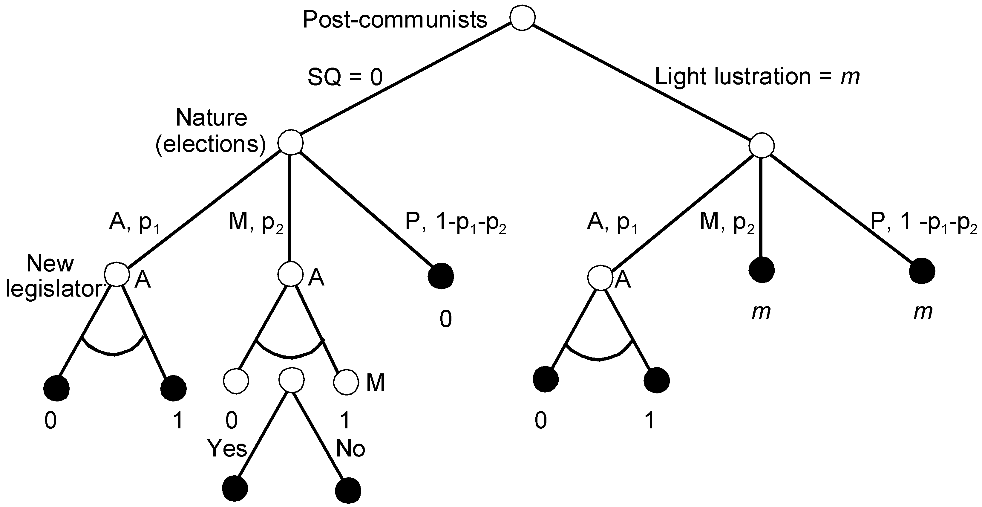
In the field of political economy, typical models are often represented as parametrized families of games (in short, parametrized games). SPE is often an appropriate solution concept. As the next example, I apply a simplified Auto-Lustration (AL) model [37], which is a more complex version of the Agenda Setter model, motivated by the surprising behavior of postcommunist parties in the 1990s. When such parties returned to power in some Central European countries, just before the end of their terms, they started legislating light auto-lustration. In other words, they were punishing their own members for being former supporters of communism! The term “lustration” signifies some punishment imposed on former functionaries or on the secret informers of communist regimes such as making their names public or blacklisting them from certain public offices.
Example 4.
Auto-Lustration.
A postcommunist party (P) and an anti-communist party (A) have Euclidean preferences over the lustration space . P’s ideal amount of lustration is zero; for A, the ideal amount is one. There is also a smaller moderate party, M, whose ideal point is slightly tilted to the right . M has no chance of winning a majority and will join a postelection coalition only with A.
The game unfolds as follows (recall that the dynamics are simplified and that the choices are restricted):
- Period 1: P is the ruling party and can choose between the status quo of no lustration (0) and a moderate amount of lustration, m, which is the ideal point of M;
- Period 2: Parliamentary elections take place and a new parliamentary median is elected with the following probabilities (for the extreme parties A and P, being a median is the equivalent of winning the majority):
- A: ;
- M: ;
- P: .
- Period 3: If P is the new median, then they do not introduce any new legislation, since any change, including reverting to 0, would result in an unacceptable loss of credibility in the eyes of their electorate.
- If A is the new median, then they can choose any law.
- If M is the new median, they coalesce with the larger partner A. M’s approval is necessary for any new law. If the existing legislation is 0, A proposes new legislation and then M must either accept or reject it. If the existing legislation is m, A proposes no new legislation, anticipating that it will not receive M’s support.
- Period 4 (only if M is the new median and the existing legislation is 0): M either accepts A’s proposal or the status quo prevails.
Figure 4 shows the AL game with the issue space or the outcomes in place of the payoffs.
The game is parametrized by two probabilities, and , and the position of the moderate party, m.
The player strategy spaces are as follows:
- ;
- ;
- .
P’s strategy includes the initial choice between light lustration m and no lustration. A’s strategy involves three scenarios of legislation, depending on what P decided earlier and whether the new median is A or their coalition partner M. When M is the new median and P did not change the status quo, M must decide whether to accept A’s proposal or to keep 0. Thus, M’s strategy is, like in the Agenda Setter model, a subset of acceptable policies that are preferred to the status quo.
The payoffs are the negative distances of the final lustration law from the parties’ ideal points. We assume that the parties are risk neutral. The game is fairly complex and asymmetric, but the calculation of SPE is straightforward with GBI. The subscripts in the partial strategy profiles denote the player who plays that particular partial strategy.
Step 1: In its terminal set of subgames, due to its position slightly tilted to the right, M prefers anything to the status quo 0, i.e., .
Step 2: The SPEs in the three subgames of Period 3 are as follows:
- 1 and 2: If A wins the majority, they propose the harshest lustration 1.
- 3: If M is the median and the status quo is 0, A proposes 1, since they know that M prefers 1 to 0.
Applying the above order of listing the subgames, (i.e., the set of partial SPEs includes exactly one partial strategy).
Step 3: P chooses between the payoffs in the perfect upgame, reducing the game to a choice between 0 and m. Introducing a light lustration law is strictly preferable if the expected payoff from playing m is higher than it is from playing 0:
After simplification,
This is the equilibrium condition for m to be concatenated to the previously obtained partial strategy profile and to form a unique SPE: . When the inequality is reversed, 0 is the newly partial strategy profile and the unique SPE is ; with equality, both 0 and m can be concatenated to form two SPEs.
In Hungary and Poland, P won the majority in the 1994 and 1993 elections only because the rightist parties were fragmented in those early elections and were unable to form a unified bloc. It was practically certain that, in the new elections, either A or M would win. Note that with and the inequality is satisfied. Light auto-lustration was a sensible strategy as insurance against the harsher punishment by the new government. In fact, in both Hungary and Poland, A won the next election but M became the new median, and despite many attempts, A was unable to strengthen the existing lustration law significantly [38].
5.5. Weakly Undominated Strategies in Subgames
A typical voting game may involve a large number of SPEs that are unreasonable. The GBI algorithm can be modified in order to eliminate such unreasonable equilibria. While the modification explained below is ad hoc, it is worthwhile to examine how it works in a specific game.
Example 5.
Roman Punishment.
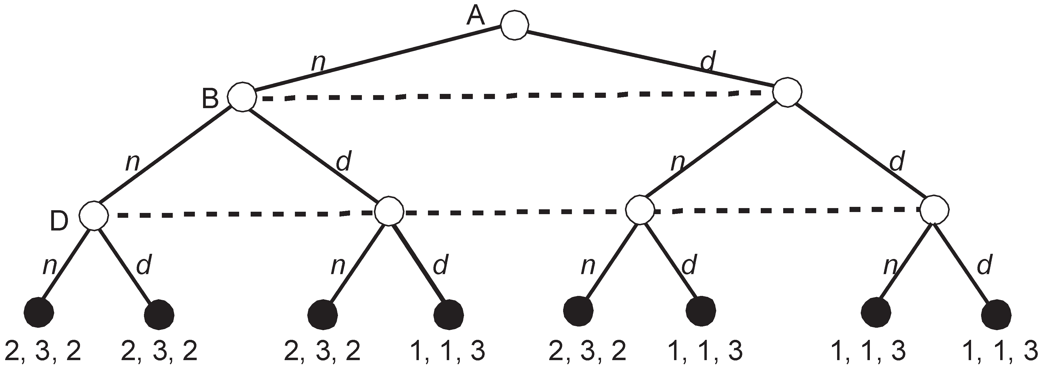
Farquharson [39] and Riker [40] analyzed the apparently first recorded case of a voting manipulation. The letter of the manipulator, Pliny the Younger, reported the story of a decision made by the Roman Senate. Three groups of senators were deciding the fate of a freedman, who was possibly involved in the death of a Roman consul. According to the Roman judiciary agenda, which was clearly quite different from the modern court procedures, the senators needed to decide first whether the freedman deserved death or not. A negative answer would trigger the next decision, whether to banish or acquit the freedman. The game analyzed below should have taken place in the Roman Senate according to its normal agenda. However, it did not happen since Pliny persuaded the senators to use a simpler plurality agenda in which they voted over the three options simultaneously.
Voting rule: simple majority, no abstention
Round 1 alternatives: d (death) or n (no death)
Round 2 alternatives (if n wins in the first round): b (banish) or a (acquit)
Players (the names correspond to the player top alternatives): A (acquiters), B (banishers), and D (death penalty supporters)
Player preferences:
- A: a preferred to b preferred to d
- B: b preferred to a preferred to d
- D: d preferred to b preferred to a
Let us convert the player preferences into payoffs in the following way:
- 3—the top alternative for every player
- 2—the second-best alternative for every player
- 1—the worst alternative for every player
Figure 5 depicts the extensive game representing voting according to the Roman agenda.
The game looks simple but the number of SPEs is staggering. H4 depicted in Figure 5 has three SPEs, i.e., = {(b; b; b), (a; a; a), (a; b; b)}. When all players vote identically, either (b; b; b) or (a; a; a), their vote is an NE (and also SPE) since no deviation of one player can change the outcome of voting. The third SPE, (a; b; b), is when all voters vote for their preferred alternative, i.e., when they choose their strategies that are weakly dominant in H4.
The remaining three subgames H1, H2, and H3 have a structure that is identical to H4 and have three SPEs each. Thus, when we prune all four subgames, the set of partial SPEs, , includes = 81 partial strategy profiles. There are = 16 possible upgames since in each subgame, either a or b, can be the equilibrium outcome with the corresponding payoff vectors (3, 2, 1) or (2, 3, 2). Thus, every subgame may be replaced either with (3, 2, 1) or (2, 3, 2).
At this moment, I abandon calculating all SPEs since the number is large and all of them except for one have a fatal flaw. Namely, except for the partial strategy profile (aaaa; bbbb; bbbb), in all other strategy profiles, at least one player plays a weakly dominated strategy in at least one subgame, i.e., votes for the second-best alternative. Let us consider what happens in the perfect upgame resulting from this special profile that steers clear of weak domination (aaaa; bbbb; bbbb) (see Figure 6).
A quick calculation shows that the players in our upgame have three SPEs similarly to the four removed subgames. In addition to (n; n; n) and (d; d; d) that involve at least one weakly dominated strategy, there is an SPE in weakly dominant strategies (n; n; d). The concatenation of this SPE with the previously obtained (aaaa; bbbb; bbbb) brings an SPE (naaaa; nbbbb; dbbbb) that has an additional property that. in all removed subgames and in the final upgame, no player plays a weakly dominated strategy.
It is straightforward to show that, in Roman Punishment, the strategy profile (naaaa; nbbbb; dbbbb) is a unique perfect equilibrium (PE). All partial strategy profiles are also unique PEs in the respective subgames. Interesting questions arise: (1) What are the general conditions for the concatenation of partial PEs to produce a global PE? (2) Can we obtain all PEs that way? and (3) Does the final result depend on the pruning sequence? Moreover, since any equilibrium concept refining the SPE can be applied at all stages of GBI, similar questions arise for all other refinements.
6. Conclusions
The contributions of this paper include the following: (a) the axiomatization of infinite games; (b) a demonstration that BIS and SPE are equivalent for such games for pure and behavioral strategies of finite support and crossing; and (c) the provision of an algorithm for solving certain games. Infinite games that I consider may have imperfect information, infinite action sets, and an infinite horizon. Informally, the algorithm operates as follows (the formal presentation is found in Section 4):
- Identify the game’s agenda, i.e., the tree consisting of all roots of the game’s subgames that is ordered by the relation of the successor imported from the game tree. Set the pruning sequence.
- Prune any subgame according to the pruning sequence and substitute its root with the subgame’s SPE payoffs. The procedure of substitution may be conducted simultaneously for any subset of agenda nodes as long as the corresponding subgames are pairwisely disjoint.
- Concatenate all partial strategy profiles resulting from the substitution.
- If at any point one receives an empty set as SPE for the subgame, this would mean that there is no SPE compatible with the set of previously selected SPEs for the subgames.
- In order to find all SPEs, one needs to try all possible substitutions of the subgames with SPE payoffs.
- One stops at the root of the game.
The examples discussed above illustrate the application of the algorithm to complex games that involve simultaneous pruning of large numbers of subgames (Example 1), continuum of actions (Example 2), behavioral strategies and imperfect information (Example 3), and parametrized games (Example 4). Example 5 shows an ad hoc modification of GBI that allows to find the unique perfect equilibrium in a game that has a large number of unreasonable SPEs.
Three open problems deserve a further comment:
- Extending the results: An obvious open question is whether the results for behavioral strategies of finite support and crossing can be generalized to all “rough” behavioral strategies. Attacking this question would demand leaving the comfortable world of finite probability distributions and using measure theory in the spirit of Aumann’s [30] pioneering contribution. The framework presented in this paper goes around measure-theoretic difficulties by assuming finite support and crossing. Both assumptions imply that the total number of terminal paths that count for calculating payoffs is finite for every strategy profile. It is easy to identify the places in the proofs where this fact is used. A natural question, then, is whether the equivalence can be extended.
- Axiomatization of noncooperative game theory: The general axiomatic framework applied in the present paper encompasses more games than the classical approaches of von Neumann [4] and Kuhn [6]. When game theory was born, it seemed natural to consider only finite games; nonfinite games rarely appeared in the literature. Today, we routinely go beyond the limitations of finite games, either with a continuum of strategies that represent quantity, price, or position in the issue space or with the infinite repetition of a game. I believe that contemporary game theory deserves sound axiomatic foundations that can cover infinite games. This would lead toward a more unified and complete discipline. Concepts that were axiomatically analyzed for finite games, such as Kreps and Wilson’s (1982) sequential equilibrium, seem to be obvious targets for a more comprehensive axiomatic investigation. The present paper demonstrates that new results or extensions of well-known results can be obtained within the general framework of infinite games.
- Modification of BI beyond subgame perfection: The final question is whether backward induction can be modified for other solution concepts beyond subgame perfection. An immediate ad hoc modification would consider only those SPEs that exclude partial equilibria with weakly dominated strategies, as it was demonstrated in Example 5. Perhaps, after a suitable modification of the main principle, backward induction-like reasoning could also produce some other refinements. On the other hand, proving that this is not the case would be an interesting finding as well.
Further refinements of backward induction could produce computational benefits similar to those obtained for subgame perfection. Backward solving is equivalent to the hierarchical concatenation of solutions. Thus, solving a game with backward reasoning is equivalent to collecting together those independent solutions and connecting the global solution with stage-wise decision-making. Arguably, this is how all decisions are made.
Funding
This research received no external funding.
Acknowledgments
Michael McBride, Michael Chwe, Drew Fudenberg, Marc Kilgour, Tom Schelling, Tom Schwartz, Harrie de Swart, Donald Woodward, Alexei Zakharov, anonymous reviewers and the participants of the IMBS seminar at the University of California, Irvine, kindly provided comments.
Conflicts of Interest
The author declares no conflict of interest.
Appendix A
Proof of Lemma 1.
The Lemma will be proved for game G. The assumptions of finite support and crossing apply to the subgames as well as to G, which means that all steps of the proof can be repeated for every subgame of G.
Part (a): The construction of a terminal path is by induction. Both when and when for , there is a node such that . Let us choose v as the second (after ) node of the path.
Let us assume that a path e of length l reached a node x. If , e is the desired path. If , let be such that . Both when and when for , there is a node such that . Path and its length is . The construction either ends at some endnode or proceeds indefinitely, producing some infinite path. In both cases, the resulting path e is terminal. By definition of the game and under the assumption of finite crossing, only a finite number of factors in the product is in the interval ; by construction, the remaining factors are equal to 1. Thus, and .
Now, let us assume that is infinite. We will construct by induction an infinite path that violates finite crossing. Path begins with . Now, let z be such that (1) crosses information sets with nondegenerate probability distributions and (2) is infinite. We will extend in such a way that the number k from (1) increases and (2) is preserved. By finite support, only for a finite number of , ; among them, for at least one t, is infinite. Let us add t to . By construction, crosses information sets with nondegenerate probability distributions. Extending this construction indefinitely, we find a path that violates finite crossing.
Part (b): If , then by definition of , for some , , which implies .
If , then, by final crossing, only for a finite number of ; for all other , . This implies .
Part (c): By (a), is finite and non-empty. The thesis is proved by induction over k, i.e., for all terminal paths with the lengths shorter or equal to k or nonterminal paths with the length equal to k included in .
First, the total probability of reaching the path of length 1 within is 1 because .
Second, let us assume that the thesis holds for all paths that are no longer than k. Let us consider all such paths that are no longer than . The sum of the probabilities of reaching the final nodes of such paths includes two subsets of terms. The probabilities that are assigned to all paths no longer than k do not change and enter the summation in the same way as is the case for all paths no longer than k. There may be new terminal or nonterminal paths with the exact length of . Here, two cases are possible. First, the probability of reaching the extra node is 1. This means that the term associated with such a path f enters the summation in the same way as for all paths no longer than k. Second, the distribution at the next-to-final node y is nondegenerate. In such a case, instead of a single path e that is no longer than k, we now have—by finite support—a finite number of paths that are no longer than and that go through y. The total probability associated to them at node y is 1. Thus, the summation term corresponding to path e is now substituted by a finite number of terms that add up to the same number. This means that the total probability of reaching the ends of all distinct paths that are no longer than is 1. Since is finite, finite crossing implies that there is a common maximum for the length of the segments, such that the associated probabilities are smaller than 1. The probabilities associated with reaching this maximum—or a shorter length if the path ends earlier—is equal to the probability distribution over and is equal to 1. □
Proof of Lemma 2.
Part (a): Every subgame H divides the set of information sets of player i into two subsets. Every can be partitioned into two partial strategies, and , defined for those two subsets the same way is defined. First, two different strategies produce two distinct pairs of partial strategies, since they must differ for at least one information set. Second, every pair of partial strategies and may result from some partition—namely, from the partition of a strategy that is identical for all information sets with the pair.
Part (b): It is a simple consequence of (a). □
Proof of Lemma 3.
A terminal path in either includes or does not include . By Lemma 1, the total number of paths in is finite; hence, () can be represented as the sum of the payoffs
We need to show that the first term in Equation (A1) is equal to the payoff of in H multiplied by the probability of reaching , the root of H.
If , then, from the definition of , we have the following:
for all
Since the summation is over a finite set, this means that (sH).
Now, let us assume that . First, notice that
- (i)
- every terminal path defines a terminal path of in H and all terminal paths of in H can be obtained this way.
Moreover, for every and the corresponding , we have the following:
- (ii)
- and
- (iii)
We can then use (i)–(iii) to make substitutions:
□
Proof of Lemma 4.
By Lemma 3, it is sufficient to show that
This follows from the fact that is identical to for all information sets outside of H and that all terminal paths for in F, with the exception of have by definition the same probabilities and payoffs assigned as in G. For , the probabilities of reaching are equal by definition; the equality follows from the definition of F as an -upgame of G. □
Proof of Theorem 1.
: decomposing an SPE strategy profile must result in a pair of SPE strategy profiles.
Since H is a subgame of G and since is an SPE in G, must be an SPE for H. We need to prove that is an SPE for F. Let us assume that this is not the case and that we can find J—a subgame of F—such that is not a Nash equilibrium. Here, two cases are possible:
Case 1: J does not include . In this case, J is disjoint with H. Thus, J is also a subgame of G and is identical with . However, implies that is a Nash equilibrium, which also must be the case for .
Case 2: J includes . Let us assume that there is a player, i, of which the strategy gives a higher payoff than , i.e.,
Let us denote () as . We will find K, a subgame of G, such that all payoffs in K are identical with the corresponding payoffs in J. Let K be defined as J, with substituted with subgame H. By construction, K is a subgame of G and is a Nash equilibrium in K. J is a (, H)-upgame of K. Let us define a new strategy profile in K as = . We now apply Lemma 4 to K; J; strategy profiles , , , and ; and player i:
and
Subtracting the respective sides of Equation (A5) from Equation (A4), we obtain a contradiction with our assumption that is an NE in K:
: every strategy profile resulting from the concatenation of SPE strategy profiles is SPE.
Let be an SPE in H, the subgame of G; be SPE in F, the -upgame of G; and let = . We need to show that is SPE.
Let us assume that this is not the case. Thus, we can find a subgame K of G such that is not a Nash equilibrium. This implies that some player i could improve their payoff against by playing some strategy , i.e.,
I will show that Equation (A7) is in contradiction with (b). Let us denote as . Three cases are possible.
Case 1: K is a subgame of F that does not include . By the subgame perfection of F and contrary to Equation (A7), must be a Nash equilibrium.
Case 2: K is a subgame of H. By the subgame perfection of H and contrary to Equation (A7), must be a Nash equilibrium.
Case 3: K includes the node and at least one more node from F. In such a case, K must include all nodes that follow and H must be a subgame of K. Let J be the -upgame of K. J is also a subgame of F. By (b), F is an SPE and both and are SPEs in H and J, respectively. By Lemma 4,
and
Proof of Lemma 5.
First, let us assume that neither the root of H follows —the root of J—nor follows . If there is a third node, , that belongs to both subgames, then, by definition of the subgame, both and must be followed by . Thus, we could find at least two different paths to : one through and one through , which is inconsistent with the definition of the tree.
Now, let us assume that follows or vice versa. However, this would imply that the path to in the agenda is longer than the path to (or vice versa) and that the subgames cannot be at the same level. □
Proof of Theorem 2.
Subgame perfection of is assumed on both sides, so we need to prove that is SPE for G iff is SPE for F.
Part 1: is finite, i.e., = {1, …, n}. Theorem 2 follows from applying Theorem 1 in both directions a finite number of times to a chain of upgames such that G = , = F, and, for , is the ( )-upgame of .
Part 2: is infinite.
:
Let us check if it is possible to to find a strategy in F for some player i that would offer a higher payoff in some subgame L of F than s. Let us denote the strategy profile (, ) as . By Lemma 1, the total number of terminal paths relevant for , , or is finite. Since all subgames with their roots in are disjoint, this implies that the number of roots in that are part of any such path is also finite. Let us denote the set of such roots as and the -upgame of G as K. Since is finite, is SPE in K by the finite part of the proof (Part 1).
Let us denote as M the subgame of K that has the same root as L. By construction of K, M=L or L is an -upgame of M. Since is SPE, is SPE, and by Part 1 of the Proof, is SPE; player i cannot receive a higher payoff with .
: The proof is similar to the part. The assumption that there exists a strategy that could improve the payoff of player i in some subgame L of G leads to a contradiction. The strategy profiles , (, ) = , and have only a finite number of paths that reach at least one of . This allows us to drop an infinite number of subgames from and to construct a smaller subgame K of L with the payoffs identical to L for respective strategy profiles , , , and such that F is an -upgame of K for some finite subset . By Part 1, is SPE for K, which means that an improvement in payoff for player i playing is impossible in K, which implies that it is also impossible for i to improve from playing in L. □
References
- Zermelo, E. Über Eine Anwendung Der Mengenlehre Auf Die Theorie Des Schachspiels. In Proceedings of the Fifth International Congress of Mathematicians, Cambridge, UK, 21–28 August 1912; Cambridge University Press: Cambridge, UK, 1913; Volume 2, pp. 501–504. [Google Scholar]
- Schwalbe, U.; Walker, P. Zermelo and the Early History of Game Theory. Games Econ. Behav. 2001, 34, 123–137. [Google Scholar] [CrossRef] [Green Version]
- Von Stackelberg, H. Market Structure and Equilibrium (Marktform Und Gleichgewicht); Springer: New York, NY, USA, 2011. [Google Scholar]
- Von Neumann, J.; Morgenstern, O. Theory of Games and Economic Behavior; Princeton University Press: Princeton, NJ, USA, 1944; ISBN 978-0-691-13061-3. [Google Scholar]
- Von Neumann, J. Zür Theorie Der Gesellschaftsspiele. Math. Ann. 1928, 100, 295–320. [Google Scholar] [CrossRef]
- Kuhn, H. Extensive Games and the Problem of Information. In Contributions to the Theory of Games I; Kuhn, H., Tucker, A., Eds.; Princeton University Press: Princeton, NJ, USA, 1953; pp. 193–216. [Google Scholar]
- Schelling, T.C. The Strategy of Conflict; Harvard University Press: Cambridge, MA, USA, 1960. [Google Scholar]
- Selten, R. Spieltheoretische Behandlung Eines Oligopolmodells Mit Nachfrageträgheit: Teil i: Bestimmung Des Dynamischen Preisgleichgewichts. Zeitschrift für die gesamte Staatswissenschaft. J. Inst. Theor. Econ. 1965, 2, 301–324. [Google Scholar]
- Rosenthal, R.W. Games of Perfect Information, Predatory Pricing and the Chain-Store Paradox. J. Econ. Theory 1981, 25, 92–100. [Google Scholar] [CrossRef]
- Selten, R. The Chain Store Paradox. Theory Decis. 1978, 9, 127–159. [Google Scholar] [CrossRef]
- Selten, R. Reexamination of the Perfectness Concept for Equilibrium Points in Extensive Games. Int. J. Game Theory 1975, 4, 25–55. [Google Scholar] [CrossRef]
- Kreps, D.M.; Wilson, R. Sequential Equilibria. Econometrica 1982, 50, 863–894. [Google Scholar] [CrossRef]
- Kohlberg, E.; Mertens, J.-F. On the Strategic Stability of Equilibria. Econometrica 1986, 54, 1003–1037. [Google Scholar] [CrossRef]
- Basu, K. Strategic Irrationality in Extensive Games. Math. Soc. Sci. 1988, 15, 247–260. [Google Scholar] [CrossRef]
- Basu, K. On the Non-Existence of a Rationality Definition for Extensive Games. Int. J. Game Theory 1990, 19, 33–44. [Google Scholar] [CrossRef]
- Bicchieri, C. Self-Refuting Theories of Strategic Interaction: A Paradox of Common Knowledge. In Philosophy of Economics; Springer: New York, NY, USA, 1989; pp. 69–85. [Google Scholar] [CrossRef]
- Binmore, K. Modeling Rational Players: Part I. Econ. Philos. 1987, 3, 179–214. [Google Scholar] [CrossRef]
- Binmore, K. Modeling Rational Players: Part II. Econ. Philos. 1988, 4, 9–55. [Google Scholar] [CrossRef]
- Bonanno, G. The Logic of Rational Play in Games of Perfect Information. Econ. Philos. 1991, 7, 37–65. [Google Scholar] [CrossRef] [Green Version]
- Fudenberg, D.; Kreps, D.M.; Levine, D.K. On the Robustness of Equilibrium Refinements. J. Econ. Theory 1988, 44, 354–380. [Google Scholar] [CrossRef]
- Pettit, P.; Sugden, R. The Backward Induction Paradox. J. Philos. 1989, 86, 169–182. [Google Scholar] [CrossRef]
- Reny, P. Rationality, Common Knowledge and the Theory of Games; Princeton University Press: Princeton, NJ, USA, 1988. [Google Scholar]
- Aliprantis, C.D. On the Backward Induction Method. Econ. Lett. 1999, 64, 125–131. [Google Scholar] [CrossRef]
- Schelling, T.C.; (University of Maryland, College Park, MD, USA). Personal communication, 2008.
- Fudenberg, D.; Tirole, J. Game Theory; MIT Press: Cambridge, MA, USA, 1991. [Google Scholar]
- Myerson, R.B. Game Theory; Harvard University Press: Cambridge, MA, USA, 2013. [Google Scholar]
- Osborne, M.J.; Rubinstein, A. A Course in Game Theory; MIT Press: Cambridge, MA, USA, 1994; ISBN 0-262-14041-7. [Google Scholar]
- Escardò, M.H.; Oliva, P. Computing Nash Equilibria of Unbounded Games. Turing-100 2012, 10, 53–65. [Google Scholar]
- Neyman, A.; Sorin, S. Stochastic Games and Applications; Kluwer Academic Publishers: Dordrecht, The Netherlands, 2003; ISBN 1-4020-1492-9. [Google Scholar]
- Aumann, R.J. Mixed and Behavior Strategies in Infinite Extensive Games; Report; Princeton University: Princeton, NJ, USA, 1961. [Google Scholar]
- Nash, J. Non-Cooperative Games. Ann. Math. 1951, 54, 286–295. [Google Scholar] [CrossRef]
- Bendor, J.; Swistak, P. Evolutionary Equilibria: Characterization Theorems and Their Implications. Theory Decis. 1998, 45, 99–159. [Google Scholar] [CrossRef]
- Flood, M.M. Some Experimental Games; Research Memorandum RM-789; RAND: Santa Monica, CA, USA, 1952. [Google Scholar]
- Brams, S.J.; Taylor, A.D. Fair Division: From Cake-Cutting to Dispute Resolution; Cambridge University Press: Cambridge, UK, 1996; ISBN 0-521-55390-3. [Google Scholar]
- Steinhaus, H. The Problem of Fair Division. Econometrica 1948, 16, 101–104. [Google Scholar]
- Romer, T.; Rosenthal, H. Political Resource Allocation, Controlled Agendas, and the Status Quo. Public Choice 1978, 33, 27–43. [Google Scholar] [CrossRef]
- Kaminski, M.M.; Nalepa, M. A Model of Strategic Preemption: Why Do Post-Communists Hurt Themselves? Decisions 2014, 21, 31–65. [Google Scholar] [CrossRef]
- Kaminski, M.M.; Lissowski, G.; Swistak, P. The “Revival of Communism” or the Effect of Institutions? The 1993 Polish Parliamentary Elections. Public Choice 1998, 97, 429–449. [Google Scholar] [CrossRef]
- Farquharson, R. Theory of Voting; Blackwell: Hoboken, NJ, USA, 1969. [Google Scholar]
- Riker, W.H. The Art of Political Manipulation; Yale University Press: New Haven, CT, USA, 1986; ISBN 0-300-03592-6. [Google Scholar]
Figure 1.
Backward induction versus subgame perfection.
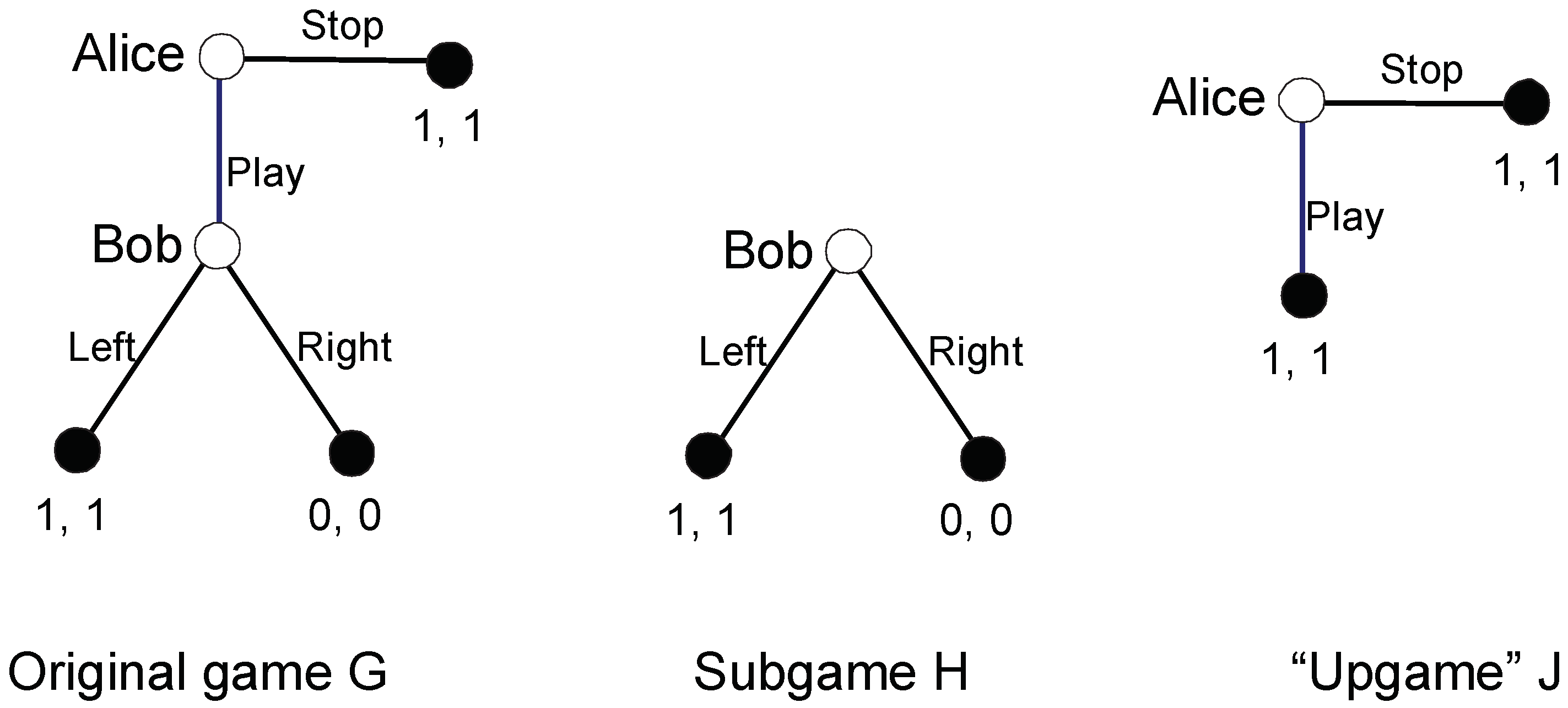
Figure 2.
Pure coordination with perfect information.
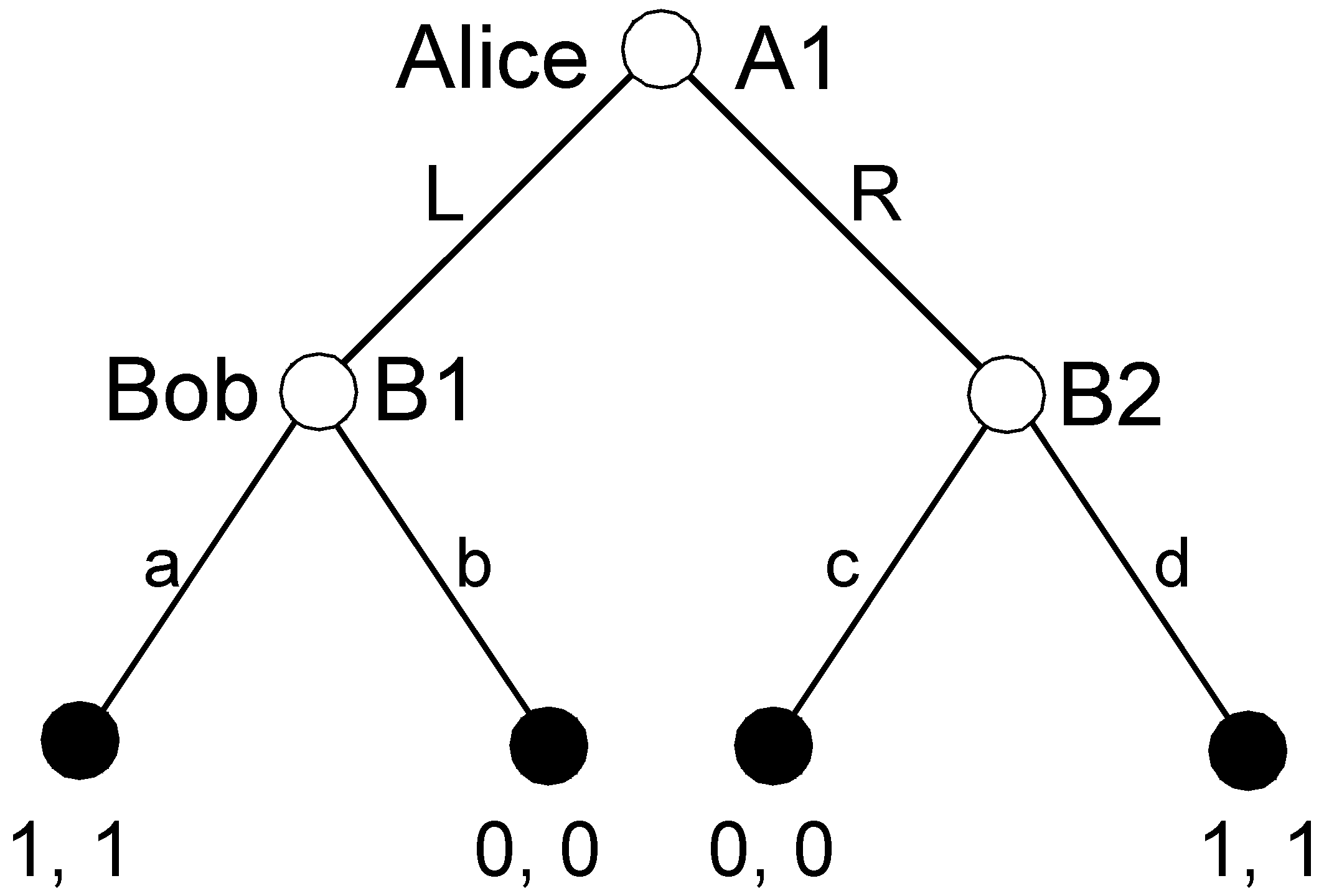
Figure 3.
The tree types of subgames pruned in Step 1.
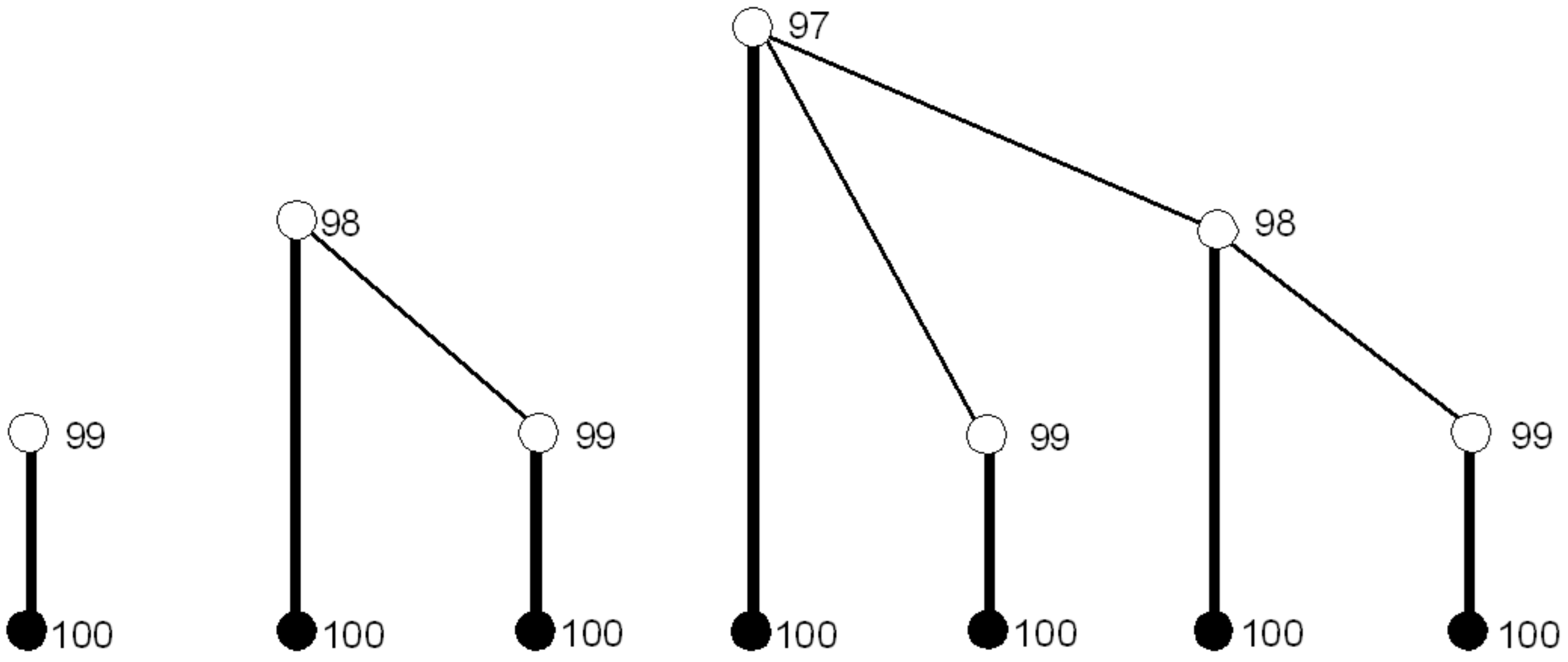
Figure 4.
Simplified structure of the Auto-Lustration game.

Figure 5.
Roman Punishment: Out of four subgames, only is shown.
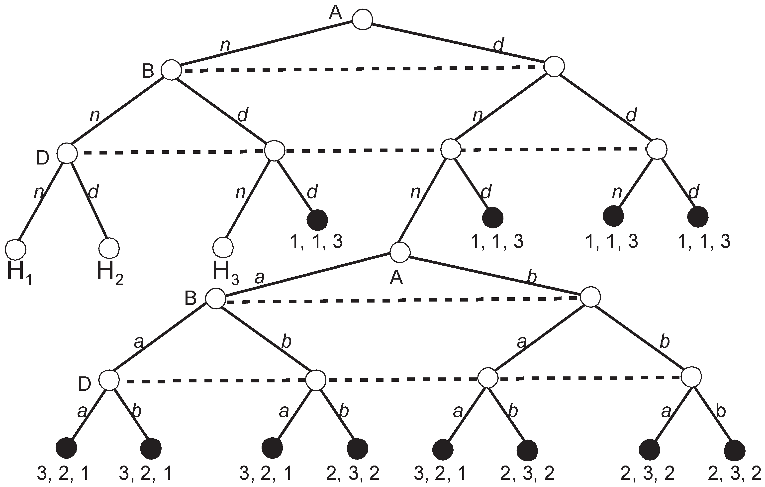
Figure 6.
The perfect upgame of Roman Punishment corresponding to (aaaa, bbbb, bbbb).

© 2019 by the author. Licensee MDPI, Basel, Switzerland. This article is an open access article distributed under the terms and conditions of the Creative Commons Attribution (CC BY) license (http://creativecommons.org/licenses/by/4.0/).
Share and Cite
MDPI and ACS Style
Kaminski, M.M. Generalized Backward Induction: Justification for a Folk Algorithm. Games 2019, 10, 34. https://0-doi-org.brum.beds.ac.uk/10.3390/g10030034
AMA Style
Kaminski MM. Generalized Backward Induction: Justification for a Folk Algorithm. Games. 2019; 10(3):34. https://0-doi-org.brum.beds.ac.uk/10.3390/g10030034
Chicago/Turabian StyleKaminski, Marek Mikolaj. 2019. "Generalized Backward Induction: Justification for a Folk Algorithm" Games 10, no. 3: 34. https://0-doi-org.brum.beds.ac.uk/10.3390/g10030034
Note that from the first issue of 2016, this journal uses article numbers instead of page numbers. See further details here.