Cost of Reasoning and Strategic Sophistication

Abstract

I designed an experiment to study the persistence of the prevailing levels of reasoning across games. Instead of directly comparing the k-level(s) of reasoning for each game, I used cognitive load to manipulate the strategic environment by imposing variations on the subject’s cost of reasoning and their first- and second-order beliefs. Subjects have systematic changes in k-level(s) of reasoning across games. That finding suggests that subjects are responsive to changes in the strategic environment. Changes in k-level(s) of reasoning are mostly consistent with the endogenous depth of reasoning model when subjects are more cognitively capable or facing less cognitively capable opponents. Subjects have cognitive bounds, but often choose a lower-type action due to their beliefs about their opponents. Finally, cognitive ability plays a significant role in subjects making strategic adjustments when facing different strategic environments.

1. Introduction

The use of the level-k model has prevailed in the literature for characterizing people’s initial responses in laboratory strategic games [1,2]. The model characterizes the player’s systematic deviations from the Nash equilibrium using a bounded rational-type explanation. The level-0 type’s action is assumed to be uniformly distributed over all actions (or in some cases, level-0 type’s action is the most prominent action available), whereas the level-1 type has the best response to the expected action of the level-0 type. The level-2 type has the best response to the expected action of the level-1 type. The iterations follow this pattern, as the level-k type always has the best response to the actions of level-$k-1$ type. Such patterns of off-equilibrium play have been evidenced in many laboratory experiments. In Nagel’s p-beauty contest game, Nagel found spikes that correspond to the first and second rounds of iterative best responses [1]. Stahl and Wilson found similar evidence of level-1 and level-2 types with 10 matrix games [2]. Camerer et al. developed a cognitive hierarchy model [3]. Instead of holding a belief that all the other players are type k-1, level-k players in the cognitive hierarchy model assign a probability distribution over all the lower types. Many other studies used the level-k model to explain laboratory data (matrix game [4]; beauty contest game [5,6,7,8]; sequential game [9]; auction [10,11]; Crawford, Costa-Gomes and Iriberri also provide a comprehensive literature review [12]).

However, although the level-k model has proven its usefulness in characterizing initial responses for many laboratory games, its predictive power remains ambiguous because (1) it is often used posteriorly to classify a player’s type given their actions and (2) the model lacks components related to individual characteristics that could help identify different types of players. It is important to understand how certain levels are reached for each individual, as it is a starting point for the discussion of the model’s predictive power. Alaoui and Penta developed a framework called the endogenous depth of reasoning (EDR) model to explain what may happen in a player’s head when they encounter a given strategic situation [13]. The EDR model captures individual characteristics by introducing cost of reasoning, which is determined both by the strategic environment and by a player’s endogenous cognitive ability. The model includes game-specific characteristics by introducing the benefit of reasoning through payoffs of the games. Lastly, the model allows a clear separation of cognitive bounds and behavioral levels observed in games by introducing higher-order beliefs. Such separation makes room for individual adjustments of k-levels in different strategic environments. As a result, a level-1 action observed from a game does not necessarily classify the player as a level-1 player. Instead, such action can be a product of the player’s cost and benefit analysis and his belief about his opponents.

The EDR model provides a plausible starting point to study the persistence of the level-k model. However, as individuals have heterogeneous costs of reasoning and belief systems in all kinds of strategic situations, it is hard to conduct direct comparisons across games to test whether the behavioral k-levels follow the EDR model’s predictions. In this paper, I use Costa-Gomes and Crawford’s two-person guessing games (henceforth CGC06) and cognitive load to create different strategic environments [14]. By controlling cognitive load, I create a standard for the cost of reasoning for all the subjects. Although individual cognitive ability may still have an effect, by using a within-subject experimental design, the individual effect will no longer impact the comparisons of strategic levels across games for the same subject. The revelation of information about the strategic environment is also carefully manipulated to clearly control the subject’s belief space. The goal was to test whether the EDR model provides directional predictions about the changes on k-levels across games for any given subject. Alaoui and Penta tested the benefit part of their model using the 11–20 money request game with altered bonus rewards [13,15]. To the best of my knowledge, this was the first paper to provide experimental tests of the EDR model by introducing different strategic environments with controlled cost and belief space.

With the 18 two-person guessing games in the experiment, the results suggest that the subject’s behavioral levels systematically vary across the games. Subjects are mostly responsive to the changes in the strategic environment. Their directional changes in behavioral levels can be predicted by the EDR model when they are more cognitively capable or their opponent is less cognitively capable. An inherent cognitive bound exists for the subjects in different strategic environments. When comparing a subject’s behavioral levels across all the games while providing the same amount of cognitive resources, their behavioral levels rarely exceed their cognitive bound level for that strategic environment.

A few other papers also studied the correlation of individual k-levels with cognitive ability. Allred et al. investigated the effects of cognitive load on strategic sophistication [16]. In their experiments, they asked the subjects to perform a memorization task of either a three- or nine-digit binary number concurrently with strategic games such as beauty contest, 11–20, and 10 matrix games. They found that subjects with high loads (i.e., nine-digit number) were less capable of computing best responses, especially for the beauty contest game. They were also aware of their strategic disadvantages. The net result of cognitive load depended on the specific strategic context. Burnham et al. used a standard psychometric test to measure the cognitive abilities of their subjects, and correlated the test results with subjects’ performances in a p-beauty contest game [17]. They found a negative correlation between cognitive test scores and entries in the beauty contest game, indicating that subjects with higher cognitive ability tend to be more strategically sophisticated in such games. Gill and Prowse used a 60-question non-verbal Raven test to assign subjects into high- and low-cognitive-ability groups [18]. They asked the subjects to play a p beauty contest game for 10 rounds, and found that subjects in the high-cognitive-ability group converged to equilibrium faster. These studies provided some evidence of the correlation of individual k-levels with cognitive ability or carefully controlled cognitive tasks. In my experiment, I used memorization tasks to manipulate the cost of reasoning for the subjects in the context of a two-person guessing game. According to Allred et al., higher cognitive load negatively affects a subject’s ability to calculate the best responses in this type of guessing games [16]. To attain a higher level of strategic sophistication, players have to exert more effort to combat the effects of cognitive load; therefore, the cost of reasoning increases with cognitive load in this strategic situation. Every subject experienced both the low and high cognitive loads at some point during the experiment, so they were fully aware of the additional cost of reasoning that was added by these memorization tasks. As a result, their cost of reasoning and their belief about their opponent’s cost of reasoning can be quantified by the cognitive load.

The stability of k-levels is an important aspect in the level-k model literature. Stahl and Wilson used twelve normal-form games to estimate the player’s level [19]. They found that using a relatively low threshold, 35 out of 48 subjects could be classified as stable across games. Fragiadakis et al. asked the subjects to repeat their decisions in a series of two-person guessing games to subsequently best respond to their past actions [20]. They found that only 40% of the subjects who were able to replicate the decisions could be classified as a known behavioral type. A few works mentioned the predictive power of strategic sophistication. Arad and Rubinstein used a multidimensional Colonel Blotto game to observe subject’s multidimensional iterative reasoning process [21]. They found that subjects with a higher level of reasoning in the 11–20 money request game also seem to have more rounds of iterative reasoning in this game.

Perhaps the most closely related work to this paper is Georganas, Healy, and Weber’s 2015 paper [22]. They conducted an experiment to examine the cross-game stability of the k-levels. They used four matrix undercutting games and six two-person guessing games and compared them at the individual level. They found no correlation between the levels of reasoning across games. However, they found some evidence of cross-game stability within the class of undercutting game. I studied a similar question to the cross-game stability of the level-k model. Instead of introducing a second family of games, I used cognitive load to mimic different strategic environments, and restricted the subjects to fixed pairs while playing the games. The belief space was therefore carefully controlled, and the uncertainty from playing against a new random player for each round was completely eliminated. The data suggested that systematic level changes can be predicted by the EDR model under certain conditions. In Section 2, I provide a brief introduction to the EDR model to cover some necessary background and theoretical predictions. In Section 3, the experimental design is introduced in detail. Section 4 and Section 5 cover the data analysis procedure and the discussion of the results, respectively. Section 6 provides the concluding remarks.

2. Theoretical Consideration

2.1. Model

I adopted Alaoui and Penta’s EDR model for theoretical predictions [13]. In this model, players follow an endogenous reasoning process that determines the strategic bound in a particular context. With added structure on beliefs, the model is able to predict a player’s actual level of play in any game that could use a k-level iterative best response reasoning process. The main benefit of using this model is that the structure of the model allowed me to conduct a comparative statics exercise on a player’s reasoning process. One of the main goals of this study was to conduct a comparative static exercise on the cost side. Below, I provide more detailed descriptions of some key features of this model. These features are relevant to the experimental design and predictions for this paper.

A player’s cognitive bound is a mapping from the incremental cost of reasoning ($c\left(k\right)$) and the incremental value of reasoning ($v\left(k\right)$) at each level to the intersection of the two terms.

$$\kappa (v,c)=min\{k\in \mathbb{N}\mid v(k)\ge c(k\left)andv\right(k+1)<c(k+1\left)\right\}$$

(1)

A player reaches their cognitive bound at the kth level by having a value of reasoning for that level exceeds cost of reasoning, but their cost–benefit analysis no longer supports the one-higher level (i.e., $k+1$) of reasoning. Further denote the cognitive bound of player i as ${\overline{k}}_i$, where:

$${\overline{k}}_i=\kappa (v_i,c_i).$$

(2)

According to Alaoui and Penta, the value of reasoning is affected by the payoff of the game [13]. The cost of reasoning is an endogenous characteristic of an individual, which is largely related to their cognitive or reasoning ability. In this paper, I take their assumption on the value of reasoning and continue to assume that the payoff is the only incentive for players to apply logical reasoning in the games. I provide a further discussion on the cost of reasoning. Beyond an individual’s endogenous ability, the strategic environment (such as cognitive load) provides many challenges for a person in applying strategic reasoning, which alters the cost of reasoning.

A player’s belief is represented as a tuple. Since the game in my design is symmetric in payoffs, a player’s belief can be restricted to the beliefs about the cost of reasoning. Therefore, the first element of the tuple, $c_i$, represents player i’s own cost of reasoning. The second element is player i’s beliefs of his opponent’s (player j) cost of reasoning, denoted as $c_j^i$. The last element $c_i^{ij}$ is player i’s second-order belief, which is their belief about player j’s belief of themselves. Any higher-order beliefs could be nested to the first- and second-order beliefs; therefore, a player’s belief is represented as:

$$t_i=(c_i,c_j^i,c_i^{ij}).$$

(3)

2.2. Theoretical Predictions

I formulated the testable predictions following the EDR construction discussed in Section 2.1. For any game $G={\{X_i,u_i\}}_{i=1,2}$, let $k_i\left(x_i\right)$ be the reflected behavioral level of player i by choosing action $x_i$, where $X_i$ is the set of actions available for player i and $u_i$ is the payoff function for player i.

• Changing the cost of reasoning: For any $c_j^i$ and $c_i^{ij}$, $k_i\left(x_i\right)$ (weakly) decreases with $c_i$. Fixing player i’s first- and second-order beliefs, their cognitive bound weakly decreases with the cost of reasoning. The observed level of player i from the game will also weakly decrease. In my design, for the first 16 games holding cognitive load and information structure constant for the opponent, players will display lower strategic levels when the memorization task is a string of seven letters.
• Changing the opponent’s cost of reasoning: For any $c_i$ and $c_i^{ij}$, $k_i\left(x_i\right)$ (weakly) decreases with $c_j^i$. If $c_i^{ij}=c_i$, then player i’s cognitive bound is binding if they regard their opponent as more sophisticated.
  Player i reacts to the change in the cost of reasoning of their opponents. More specifically, if he observes his opponent’s cost of reasoning increasing, he will adjust their strategy in the game to best respond to his opponent. That means they may choose to take an action that corresponds to a lower level of strategic sophistication. However, such adjustments of strategies are binding by the cognitive bound when the player believes their opponent has a lower cost of reasoning compared to their own cost. In the context of my experiment, a player should choose a weakly lower level of strategy if he observes his opponent’s memorization task becoming more difficult (i.e., from a string of three letters to a string of seven letters).
• Changing the second-order belief: For any $c_i$ and $c_j^i$, $k_i\left(x_i\right)$ (weakly) decreases with $c_i^{ij}$. If $c_i\ge c_i^{ij}$, then player i’s cognitive bound is binding. By fixing player i’s own cost of reasoning and his opponent’s cost, through only changing player $i^{\prime }$s second-order belief, player i should adjust their strategic actions. For example, when a player has a low cost of reasoning in the game, if they believe that their opponent has a wrong belief about themselves, namely, they believe that their opponent thinks the cost of reasoning for them is very high, then they can switch to an action that is associated with a lower level of reasoning. However, this adjustment of strategic actions according to the second-order belief is restricted by player i’s own cognitive bound, meaning that they cannot make any adjustments that requires a higher level of reasoning than their cognitive bound. In the context of my experimental design, players should adjust their actions when the information structure shifts from full revelation of cognitive load to partial revelation.
• Cognitive bound: Given $c_i$, for any $c_j^i$ and $c_i^{ij}$, $k_i\left(x_i\right)$ never exceeds ${\overline{k}}_i$. When fixing player i’s own cost of reasoning, their behavioral level should never exceed their cognitive bound. In the context of this experiment, on an individual level, actions observed in games 17 and 18 should correspond to the highest level of reasoning that one player can achieve under the respective cognitive load.

3. Experimental Design

In this section, I present the details of the experimental design. The experiment captured the process of level-k thinking through the two-person guessing game [14]. I provide a brief introduction to the game first, followed by the treatment design and the experimental timeline.

3.1. The Game

The two-person guessing game is an asymmetric, two-player game. Each player has a lower limit, $a_i>0$, an upper limit, $b_i>0$, and a target $p_i\in (0,2)$. Players are required to input a guess that is within their lower and upper limit. However, their actual choice is not restricted by the limit. Denote player i’s input by $x_i$. If a player guesses a number $x_i$ that falls outside the limit interval, then their guess will be adjusted to the closest bound. For example, if $x_i<a_i$, then the adjusted guess $y_i$ will be $y_i=a_i$. If $x_i>b_i$, then the adjusted guess $y_i$ is $y_i=b_i$. However, any guess falling within the limit interval will not be adjusted; i.e., $y_i=x_i$.

The goal of the game is to make a guess that minimizes the difference between the player’s own guess and the product of their target and his opponent’s guess. Denote the difference by $e_i=\mid y_i-p_i·y_j\mid$. The payoff is a quasi-concave function minimized at zero. Player i receives $u_i=max\{0,200-e_i\}+max\{0,100-\frac{e_i}{100}\}$. Since a player’s guesses that have the same adjusted inputs will yield the same outcome for the subject, I use the adjusted guess $y_i$ as a proxy of how players perform in the game.

In this game, the level-0 player is assumed to play randomly according to a uniform distribution over the action space. Denote the theoretical predicted guess made by a k-level player as $x_i^k$. Given the assumption imposed on the level-0 player’s strategy, level-1 players will best respond to the expected value of level-0 player’s guess, i.e., $x_i^1=p_i·\mathbb{E}\{y_j\mid y_j\in [a_j,b_j]\}$. The level-2 player’s strategy will then be $x_i^2=p_i·\{\mathbb{1}(x_j^1\in [a_j,b_j])·x_j^1+\mathbb{1}(x_j^1<a_j)·a_j+\mathbb{1}(x_j^1>b_j)·b_j\}$. The reasoning process follows iterative best responses. It converges to the Nash equilibrium after finite rounds of iterations.

In this paper, I adopt 14 two-person guessing games used by CGC06 and 4 two-person guessing games used by Georganas et al. [14,22]. The parameters of each game are given in

Table 1. The eighteen two-person guessing games.

Game	P1’s Limits	P2’s Limits	Treatment	P1’s Role	P2’s Role	Steps	Eqm at
#	& Target	& Target				to Eqm	Boundary
1	[(100,900); 1.5]	[(300,500); 0.7]	[LL+]	role B	role A	5+	-
2	[(300,900); 1.3]	[(100,500); 0.7]	[HL-]	role B	role A	5+	lower
3	[(300,900); 1.3]	[(300,900); 1.3]	[HH+]	role B	role A	3	upper
4	[(300,900); 0.7]	[(100,900); 1.3]	[LH+]	role A	role B	5+	lower
5	[(100,500); 1.5]	[(100,500); 0.7]	[LH-]	role B	role A	5+	upper
6	[(100,500); 0.7]	[(100,900); 0.5]	[HL+]	role A	role B	5	lower
7	[(100,500); 0.7]	[(100,500); 1.5]	[LH-]	role A	role B	5+	-
8	[(300,500); 0.7]	[(100,900); 1.5]	[LL+]	role A	role B	5+	upper
9	[(100,500); 0.7]	[(300,900); 1.3]	[HL-]	role A	role B	5+	-
10	[(300,500); 0.7]	[(100,900); 0.5]	[HH-]	role B	role A	3	lower
11	[(100,500); 1.5]	[(100,900); 0.5]	[LL-]	role B	role A	5+	-
12	[(300,900); 1.3]	[(300,900); 1.3]	[HH+]	role A	role B	3	upper
13	[(100,900); 1.3]	[(300,900); 0.7]	[LH+]	role B	role A	5+	-
14	[(100,900); 0.5]	[(300,500); 0.7]	[HH-]	role A	role B	4	-
15	[(100,900); 0.5]	[(100,500); 0.7]	[HL+]	role B	role A	4	lower
16	[(100,500); 0.5]	[(100,500); 1.5]	[LL-]	role A	role B	5+	lower
17	[(100,900); 1.3]	[(100,500); 0.5]	L	-	-	5+	-
18	[(100,900); 1.5]	[(100,500); 0.7]	H	-	-	5+	-

. All the players survive at least two rounds of iterative best responses before reaching the equilibrium (as stated in Table 1 “steps to eqm” column). Since in CGC06, only a few number of subjects reached level 3 in the reasoning process, the choice of parameters in this paper should be sufficient to identify a player’s strategic levels in the game.

3.2. Cognitive Load

Before directed to the guessing game, subjects were required to memorize a string of letters and were told that they need to recall the given string after the guessing game. The string was composed of either three or seven random letters, for example, UMH or WIEZOFH. The subjects were given 15 s to memorize the string; then they were automatically directed to the guessing game.

I did not pay the subjects specifically for correct recalls. However, their payments on the guessing game were partially dependent on this memorization task. If the recall for the selected payment round was wrong, they were not paid for that round, and left the experiment with only the participation fee. Said payment scheme incentivized the subjects to memorize the cognitive load correctly, and therefore guaranteed the effects of different cognitive load treatments.

3.3. Treatments

The experiment consisted of two blocks. In the first block, subjects were assigned into pairs. They played 16 two-person guessing games against each other within the fixed pairs. In the second block, they played two guessing games against the computer. There were a total of 18 two-person guessing games for them to complete for this experiment, and no feedback was given throughout the process.

3.3.1. Against Human

I adopted a $2\times 2\times 2$ design. For ease of explanation, I specify the two players in the guessing game as having role A and role B in this section. However, subjects were not aware of their role during the experiment. Each subject was given the role of A or B for each treatment exactly once. I used a within-subject design.

To examine the effects of changing the cost of thinking on a subject’s level of reasoning, I varied the cognitive load for role A, holding role B’s cognitive load constant. As mentioned in the previous section, role A needed to memorize a string of either three or seven random letters when playing the guessing game. To test the effects of changing the opponent’s cost of thinking on a player’s level of strategic sophistication revealed in the game, I also varied role B’s cognitive load by two levels. Changing the cost of thinking of role B essentially tests the effects of changing the first-order belief for role A. Denote the cognitive load of three letters as low load (L) and seven letters as high load (H).

Lastly, I varied the disclosure of information on the cognitive load for role B. The exact cognitive load implemented on role A was either fully revealed to role B or partially revealed as a probability distribution. Denote full revelation as [+] and the counterpart as [-]. In the partial revelation treatment, role B was told that role A has a 0.5 probability of memorizing a string of three letters and a 0.5 probability of memorizing a string of seven letters. The full and partial revelations of the cognitive load information on role B were a method of measuring the effects of changing the second-order belief for role A. In the full revelation treatment, both roles A and B were aware that role A’s memorization task is common knowledge. However, in the partial revelation treatment, role A knew their exact memorization task was hidden to role B; therefore, their second-order belief (i.e., their belief about role B’s belief of their own cost of thinking) may not coincide with their actual cost of reasoning. A summary of treatments is provided in

Table 2. The eight treatments.

	Role	Label	Cost	1st Order Belief	2nd Order Belief
1	Role A	[LL+]	Low	Low	Low (full revelation)
	Role B		Low	Low	Low (full revelation)
2	Role A	[HL+]	High	Low	High (full revelation)
	Role B		Low	High	Low (full revelation)
3	Role A	[LH+]	Low	High	Low (full revelation)
	Role B		High	Low	High (full revelation)
4	Role A	[HH+]	High	High	High (full revelation)
	Role B		High	High	High (full revelation)
5	Role A	[LL-]	Low	Low	50% Low, 50% High (partial revelation)
	Role B		Low	50% Low, 50% High	Low (full revelation)
6	Role A	[HL-]	High	Low	50% Low, 50% High (partial revelation)
	Role B		Low	50% Low, 50% High	Low (full revelation)
7	Role A	[LH-]	Low	High	50% Low, 50% High (partial revelation)
	Role B		High	50% Low, 50% High	High (full revelation)
8	Role A	[HH-]	High	High	50% Low, 50% High (partial revelation)
	Role B		High	50% Low, 50% High	High (full revelation)

. In later sections, I used role A’s label to identify the treatments, as I was essentially examining the treatment effects for role A only. The first letter in the label indicates role A’s cognitive load (either L or H). The second letter indicates role B’s cognitive load (opponent’s cognitive load, either L or H), and the last element of the label indicates full or partial revelation (role A’s second order belief, either [+] or [-]). Role B served as a supporting role to complete the information required for each treatment. The information presented to role B for each treatment is also presented in Table 2. However, when later discussing the experimental results, I only refer to each treatment using role A’s label. Table 1 provides a summary of treatments and assignments of roles for each game. Each subject played as either role A or role B exactly once for each treatment. There are in total 16 games. For each treatment, the pair of games are symmetric in game parameters and cognitive load realizations. The games were played in two random orders (the first order was as game numbers listed in Table 1; the second order was: 2, 13, 14, 4, 3, 1, 16, 6, 11, 8, 12, 5, 10, 15, 7, 9, 18, 17. Since for each game, there were two players assigned with different cognitive loads, considering player 2’s order of play, there were essentially four sequences. The number of subjects in each order was roughly balanced. After dropping subjects with missing data, there were 28 subjects playing the first order as player 1, 29 subjects playing the first order as player 2, and 27 subjects playing the second order as player 1 and player 2 respectively.). Before the start of each session, one of the two was randomly selected.

3.3.2. Against Computer

Subjects played against the computer for the second block of the experiment. The computer always chooses a Nash equilibrium action. The concept of equilibrium was explained to the subjects. For example, subjects were told that “a combination of guesses, one for each person, such that each person’s guess earns them as many points as possible, given the other person’s guess, is called an equilibrium guess.” A similar description of equilibrium guess is found in CGC06. Subjects were also given an example of an equilibrium guess following this description. However, they were not specifically taught how to derive an equilibrium guess. The reason for introducing the equilibrium concept was to encourage the subjects to perform as many rounds of iterative best responses as possible. The two guessing games in this part are labeled 17 and 18 in Table 1.

3.4. Experimental Timeline

A total of 111 subjects were recruited for this experiment. Sessions were conducted at the Incentive Lab at Rady School of Management, University of California—San Diego (San Diego, CA, USA). The experiment was programmed and conducted using z-tree [23]. The complete session lasted for 90 min. Subjects were given a 5 USD show-up fee for attending the experiment and an additional $5 if they passed the understanding test and completed the experiment. They earned an additional $8 on average depending on their decisions for the guessing games. For those who did not pass the understanding test, they spent about 30 min in this experiment and left with the $5 show-up fee.

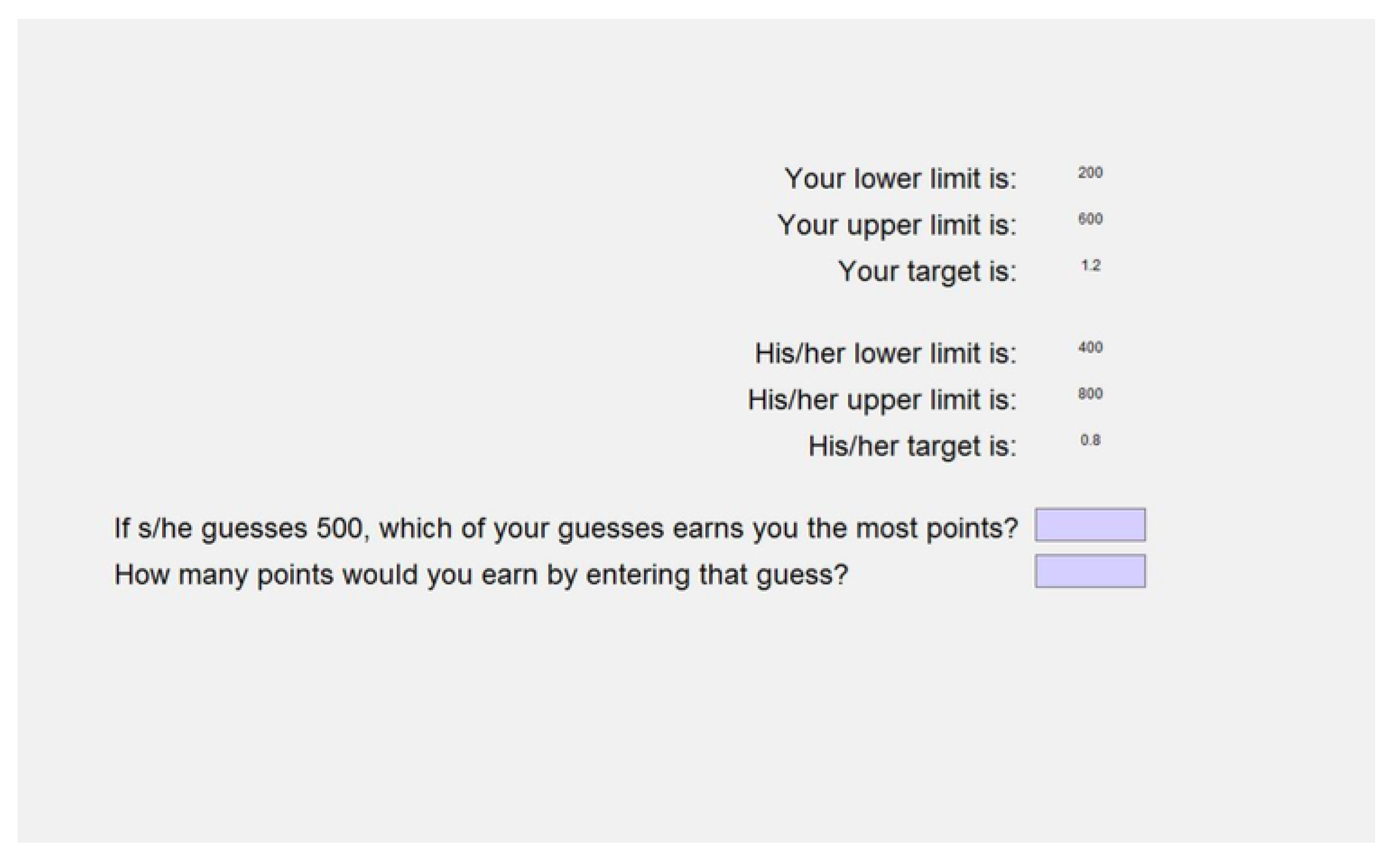
Subjects were given instructions on the two-person guessing game first. After explaining the rules, I introduced four unincentivized practice rounds. During the practice rounds, subjects played against the computer and were told that the computer will always choose the mean of the target interval. After the subjects made a guess, feedback was provided for the subjects to reflect on the game rule and the payoff rule. An understanding test was then administered. The test was composed of six questions, similar to the understanding test in CGC06. Standard questions included calculatiosn of best responses and payoffs. Although subjects in the experiment were not restricted to following a level-k reasoning process, for the purpose of the experiment, I wanted to make sure the subjects were capable of calculating the best responses. A screenshot of the understanding test is shown in Figure 1. Subjects needed to answer four out of six questions correctly to proceed to the main part of the experiment.

Before playing the incentivized guessing games, subjects were introduced to the memorization task. They were given two unincentivized practice rounds for the low load and high load treatments. During the practice round, they had the standard 15 s to memorize the string of letters and were asked for immediate recall when the time was up. They, however, did no get to practice the guessing game with the cognitive load implemented.

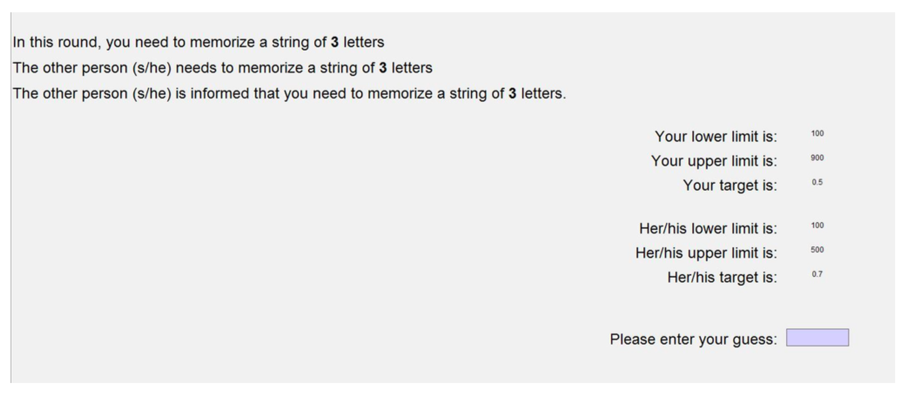
The main experiment consisted of two parts, as discussed in Section 3.3. There were 18 two-person guessing games in total. For the first 16 games, subjects were randomly assigned into pairs and stayed within the same pair for all 16 decisions (one as player 1 and the other as player 2). For each game, subjects were given the same information set that consisted of the types of memorization task (either string of three or seven letters, or a probability distribution) for themselves and their opponents, whether their opponents knew about their exact memorization task, and the targets and limits for both players. An example of the actual decision screen is provided in Figure 2. Subjects were also asked to elicit their opponents’ types of memorization task after they made their guesses and recalled the letters. This practice allowed me to check whether the subjects received and processed the correct information about their strategic environment. There was no feedback given in between the 18 guessing games. This prevented the subjects from learning anything about their opponents’ past actions. Such practice also limited the subject’s learning of the guessing game, as no payoff information was provided. (There was limited learning of the game. Upon checking a subject’s levels with respect to the orders of the games they played, playing a later game was not associated with higher k-levels. The coefficient from the OLS regression was 0.005 and it was not statistically significant.)

Subjects took a 10-question Mensa practice test at the end of the experiment. The test is used to measure the subject’s analytical ability. Some questions ask the subject to identify the missing element that completes a sequence of patterns or numbers. Some questions are verbal math questions. A couple of studies in economics literature have used a similar test as a measure of cognitive ability [22]. I used this test in the experiment to measure whether there were any heterogeneous treatment effects on subjects with different exogenous cognitive abilities.

3.5. Discussion of the Experimental Design

First, I used letters to compose strings for the cognitive load treatment, unlike the conventional use of binary numbers [16]. This design restricts the subjects from using the cognitive load numbers as their inputs for the guessing game. It allows a clear separation of the two tasks, the memorization task and guessing game, and therefore increases the reliability of the treatment effects of cognitive load. I recognized subjects may be able to use other methods to memorize the string of letters, for example, using hand gestures. However, any such method also requires cognitive effort and therefore should not significantly lessen the effects of cognitive load for treatment purposes.

Subjects remained within the fixed pair for the first 16 incentivized guessing games. Since no feedback was given in between games, this design ensures the manipulation of cognitive load being the only source of changing beliefs for any subject. Subjects were different exogenously in terms of cognitive ability, so by staying in the same pair, they carried the same beliefs about their opponents’ cognitive abilities throughout the whole session.

Lastly, for each of the 18 incentivized tasks, subjects were given 90 s to make a decision for the guessing game. According to Agranov et al., 90 s is enough for strategic players to make a decision in this type of guessing game [24]. To keep the effect of cognitive load constant across players, I only allowed the subjects to submit their guesses after the 90 s was up. Said practice avoids some subjects naïvely picking a guesses without strategic contemplation for the purpose of achieving correct recalls for the memorization task.

4. Data Analysis Procedure

All the subjects played 18 games in total, each against a fixed opponent during the experiment. There were 1998 observations of guesses. Grouping the guesses by games, I looked for level shifts observed with raw guesses. This exercise provided a general view of the effects of cognitive load on the games. I also used density plots of the guesses to visualize the treatment effects.

After the exploration of raw guesses, I estimated the level for each guess using the maximum likelihood method. Instead of assuming the subject’s behaviors are determined by a single type across all the games, I assumed the subject’s behavior in each game was determined by a single type and the types across games were allowed to be different. This was achievable with the design of my experiment with the variations on cognitive load.

Out of 1998 observations, 831 guesses correspond to a type’s exact guesses. As about 40% of the observed guesses were a type’s exact guesses, I followed the CGC06 approach in my estimation. Specifically, for each player i, game g, and level k, if player i was not making a type’s exact guesses in game g, then I defined a likelihood function $L(y_{ig}\mid k,\lambda )$ for each level k for the player in that game, with beliefs $f_g^k\left(y\right)$ and sensitivity parameter $\lambda$, based on the assumption that they were trying to maximize their expected utility.

Formally, let $x_{ig}$ be the raw guess observed for player i in game g. With the specification of lower limits $a_{ig}$ and upper limits $b_{ig}$, the adjusted guess is then $y_{ig}=min\{max\{a_{ig},x_{ig}),b_{ig}\}\}$. The density $f_g^k\left(z\right)$ represents a subject’s belief about his opponent’s action given their behavioral level being k. Although in the literature a subject’s belief of the other player’s level could follow a certain type of distribution, for example, Poisson distribution as in Camerer et al. (2004), in this study, I followed the standard approach that level-k player has point belief about his opponent, that his opponent is level-$(k-1)$ with probability 1. $y_g^0$ is defined as uniformly spread across the action space. The expected payoff of playing $x_{ig}$ with behavioral level k’s belief is then:

$$U_{ig}^k\left(y_{ig}\right)={\int }_1^{1000}{U}_{ig}(y_{ig},z)f_g\left(z\right)dz.$$

(4)

Let $U_{ig}^k=[max(y_g^k-0.5,a_{ig}),min(y_g^k+0.5,b_{ig})]$ be the interval of a type-k subject’s exact adjusted guesses, allowing an error of 0.5. Any guess for game g, subject i, who is placed within $U_{ig}^k$, is then identified as an exact match for k-level. Conversely, define ${U_{ig}^k}^{\complement }=[a_{ig},b_{ig}]/U_{ig}^k$ as the complement of $U_{ig}^k$ within the limit interval for subject i’s game g. The likelihood function is then the following:

$$L\left(y_{ig}\right|k,\lambda )=\frac{exp\left[\lambda U_{ig}^k\left(y_{ig}\right)\right]}{{\int }_{{U_{ig}^k}^{\complement }}exp\left[\lambda U_{ig}^k\left(w\right)\right]dw}.$$

(5)

Since only one observation was used for the estimation, I took the sensitivity parameter ($\lambda$) as 1.33, which is the averaged estimated value of $\lambda$ in CGC06 with only the subject’s guesses. The maximum likelihood estimate of a subject’s behavioral level in each game maximizes (5) over k, which is:

$$k_{ig}=\underset{k\in \{1,2,3,4,5,6\}}{arg\; max}{L}^{*}\left(y_{ig}\right|k).$$

(6)

To examine the treatment effects on behavioral levels, I pooled guesses into pairs for comparison. For example, to test the prediction on the changing cost of reasoning, I first identified games with the same first-order belief (either low or high cost of reasoning for opponent) and the same second-order belief (partial revelation), and then they were separated into comparison pairs by the subject’s cognitive load tasks. The same selection was performed following the conditions listed in each testable prediction.

For each pair of games, I first conducted a binary comparison on their behavioral levels and I report the summary statistics. Since this is essentially a repeated measure of behavioral level from the same sample, I then conducted the Wilcoxon signed-rank test to check the distribution of behavioral levels. Lastly, I ran a GLS random effect regression to examine the treatment effects on behavioral levels. The regression was run by regressing the estimated level on the treatment variable. A subject’s cognitive load was coded as 0 when it was in the low load treatment, and 1 when it was a high-load treatment. The same binary coding was also applied to the opponent’s cognitive load treatment. The full revelation of information treatment was coded 0, whereas partial revelation was coded 1.

5. Results

5.1. General Examination of Raw Guesses

There were a total 1998 observations and 831 guesses corresponded to a specific level (levels 1 to 5, and equilibrium). When identifying levels, I assigned the lowest possible level to a guess that matched multiple types. For example, in game 3, equilibrium was reached after three rounds of iterative best responses, and the equilibrium was at the boundary of the target interval. In this case, although levels 3, 4, and 5, and the equilibrium all have corresponding guesses at 900, a subject’s guess of 900 only assigned the subject to type level 3. This method of identification restricted over-assignments of the types.

Figure 3 shows the distribution of guesses that matched specific levels. Of the 831 guesses that matched a specific level, 43.92% were level 1 guesses, 31.41% were level 2 guesses, 14.20% were equilibrium guesses, and level 3 and higher corresponded to the remaining 10% of the guesses. To provide a clearer picture of the treatment effect, I used a Markov matrix for some treatments with these exactly matched guesses.

Table 3. Markov matrix of level transitions for increasing cost of reasoning, opponent with high load.

↓ to →	Level 1	Level 2	Level 3	Level 4	Level 5	Eqm	Num
Level 1	83.33%	0	16.67%	0	0	0	12
Level 2	25%	62.5%	12.5%	0	0	0	8
Level 3	0	0	100%	0	0	0	1
Level 4	0	0	0	0	0	0	0
Level 5	0	0	0	0	0	0	0
Eqm	0	66.67%	33.33%	0	0	0	3

and

Table 4. Markov matrix of level transitions for changing first-order belief, subject with low load.

↓ to →	Level 1	Level 2	Level 3	Level 4	Level 5	Eqm	Num
Level 1	62.5%	7.5%	2.5%	0	15%	12.5%	40
Level 2	3.7%	85.19%	7.41%	0	0	3.7%	27
Level 3	0	0	0	0	0	0	0
Level 4	0	0	0	0	0	0	0
Level 5	0	0	0	0	0	0	0
Eqm	31.25%	18.75%	28.13%	0	21.88%	0	32

present the level transitions between comparable games. For example, Table 3 consists of all the comparable pairs of changing a subject’s own cost of reasoning, fixing the opponent with a high cognitive load (game 7 [LH-] and game 14 [HH-]). There were a total of 111 pairs of comparisons, 24 of which had both guesses that exactly matched a specific level. From games 7 to 14, 12 subjects reached level 1 in game 7 and 83.33% stayed at level 1 in game 14. Eight subjects reached level 2 in game 7, 87.5% of which stayed at level 2 and below in game 14. This result largely complies with the theory prediction that increasing cost of reasoning while fixing first- and second-order belief constant decreases the level of reasoning weakly. Likewise, Table 4 presents all the comparison pairs of changing the subject’s first-order belief while fixing their own cost of reasoning and keeping their second-order belief constant (game 1 [LL+], game 8 [LL+], game 4 [LH+], and game 15 [LH+]). There were a total of 444 pairs of comparison, 99 of which had both guesses matched to a specific level. Forty pairs had level 1 guesses in the [LL+] treatment and 62.5% of them remained level 1 in the [LH+] treatment games. Similarly, 27 pairs had level two guesses in the [LL+] treatment. When changing the subject’s first-order belief by increasing the cognitive load of their opponents, about 90% of these pairs had level 2 or lower guesses in the [LH+] treatment. These statistics largely coincided with the theoretical prediction—with increasing the cost of reasoning for the opponents, the subjects adjusted by weakly decreasing their behavioral levels of playing the game. Due to the limited number of exact matches, I was not able to conduct the same exercise for all the treatment pairs. However, complete discussion of the treatment effects is provided below with estimated behavioral levels.

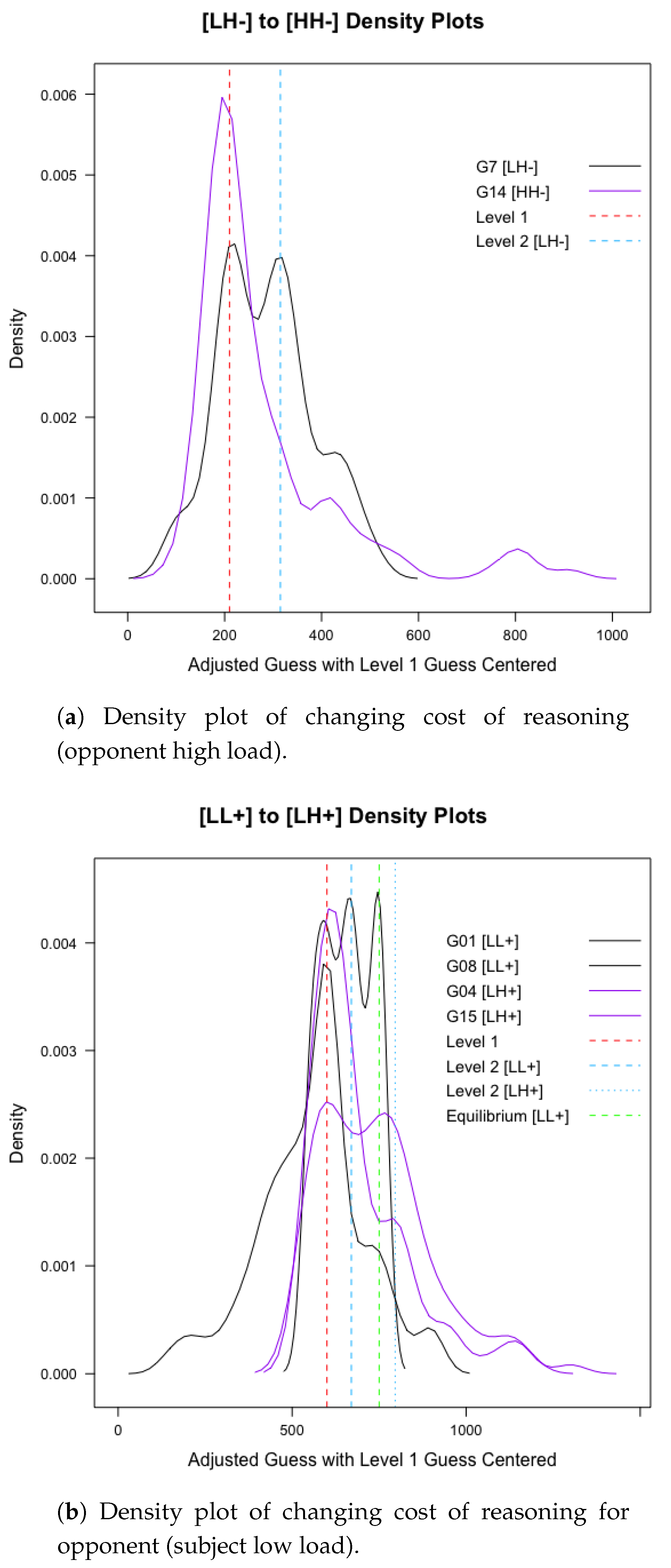
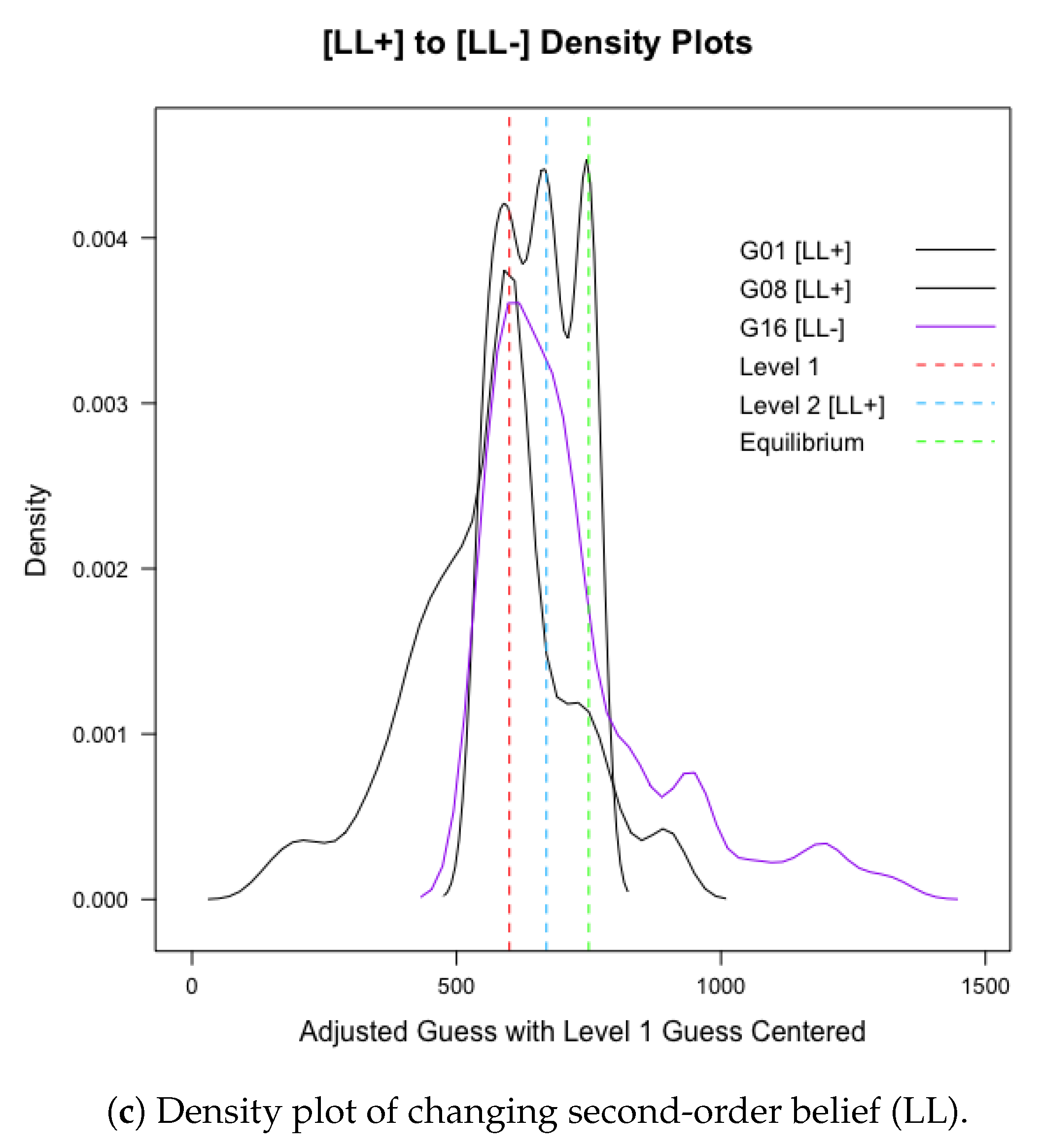
The pattern of subjects’ adjustments to the changing strategic environment is also illustrated with density plots of each game. This time, all the raw guesses (after adjustments according to upper and lower limits) were used to plot the graphs. Figure 4 illustrates the treatment effects for the three theoretical predictions. To better compare across games, level 1 guesses were centered, and all the guesses were adjusted accordingly. The colored vertical lines illustrate the level-exact guesses. For example, in Figure 4a, the vertical red dashed line indicates level-1 guesses. Both density plots in the figure show peaks around the red vertical line, which indicate higher proportions of level-1 (or close to level 1) strategy used within the games across all the subjects. Notably, in the density plot for the [LH-] treatment (G7), there is another peak centered right at the level 2 guess for that game (indicated by blue dashed line). The density plot clearly shows that in the game where subjects have a lower cost of reasoning ([LH-]), guesses are congregated at both levels 1 and 2, whereas in the game where subjects have a higher cost of reasoning ([HH-]), only a peak at the level-1 guess is observed. Likewise, in Figure 4b, four games are plotted to illustrate the treatment effects of increasing cost of reasoning for the opponent. In Figure 4c, three games are used to demonstrate changing second-order beliefs. Note that both games 1 and 8 are relevant in both graphs, as the [LL+] treatment is relevant for both comparisons. As illustrated in the figure, in one of the games, the three peaks correspond to level 1, level 2, and equilibrium. When increasing the cost of reasoning for the opponent, the level 1 peak is still observable; however, only one game has a level-2 peak. Similarly, when changing the second-order belief from low load with probability 1 to (0.5, 0.5; L, H), only the level 1 peak remains, as then the subjects thought that their opponents thought there was a 50% probability that the subject was experiencing a high cognitive load. I omitted other vertical lines that indicated different levels due to the absence of peaks in the density plots.

5.2. Distribution of Levels

From the preview of results from raw guesses in the previous subsection, changing the strategic environment appeared to lead to some structured changes in the depth of reasoning. However, only about half of the guesses were type-exact guesses. To better understand the treatment effects of the other half, I used maximum likelihood estimation to assign types, and then conducted analyses based on the estimated levels.

There were a total 1998 observations of guesses. As discussed in the previous section, I assigned a behavioral level for each observation. Surprisingly, a few guesses corresponded to exact level 4 and level 5 guesses in my data. Therefore, I included levels 1 to 5 and the Nash equilibrium type in my estimation. Of all the observations, 1167 guesses were estimated. The distribution of estimated levels for these guesses is shown in

Table 5. Summary of estimation results.

	L1	L2	L3	L4	L5	Nash
Exact	43.92%	31.41%	5.54%	1.56%	3.37%	14.20%
Estimated	71.89%	5.57%	12.94%	5.57%	3.43%	0.60%
Total	60.26%	16.32%	9.86%	3.90%	3.40%	6.26%

. The majority of the guesses were assigned to level 1 guesses. The level distribution for all the guesses is shown in

Table 6. The frequency of levels by game.

Game #	L1	L2	L3	L4	L5	Nash
All Guesses	60.26%	16.32%	9.86%	3.90%	3.40%	6.26%
1	72.97%	13.51%	0	2.70%	4.50%	6.31%
2	35.14%	16.22%	19.82%	15.32%	3.60%	9.91%
3	44.14%	22.52%	33.33%	0	0	0
4	63.06%	14.41%	1.80%	7.21%	13.51%	0
5	72.07%	12.61%	0	1.80%	0	13.51%
6	83.78%	4.50%	2.70%	9.01%	0	0
7	53.15%	12.61%	16.22%	5.41%	6.31%	6.31%
8	62.16%	12.61%	1.00%	0	0	24.32%
9	59.46%	6.31%	18.02%	1.80%	7.21%	7.21%
10	54.05%	45.95%	0	0	0	0
11	69.37%	10.81%	7.21%	1.80%	1.80%	9.01%
12	44.14%	23.42%	32.43%	0	0	0
13	70.27%	16.22%	1.00%	1.00%	5.41%	6.31%
14	73.87%	11.71%	14.41%	0	0	0
15	65.77%	15.32%	11.71%	7.21%	0	0
16	64.86%	16.22%	5.41%	2.70%	10.81%	0
17	34.23%	28.83%	3.60%	10.81%	2.70%	19.92%
18	62.16%	9.91%	9.91%	3.60%	5.41%	9.91%

. The game number is referred to the game number list in Table 1. Since all the subjects played each game exactly once, for each game listed, there were 111 observations.

The distributions of the levels were fairly similar to the results in CGC06, except that levels 4 and 5 were then included. Level 1 was the most prominent behavioral level. Of 1998 observations, 60.26% were level 1 guesses. In some games, level 1 was even more frequently observed. For example, in game 1, about 70% of the guesses were classified as level 1. A number of observations were levels 2 and 3 and Nash guesses. In my data, the occurrence of level 3 was more frequent in a few games. For example, in game 2 and game 3, more than 20% of observations were assigned to level 3. Although some observations corresponded to exact level 4 or level 5 guesses, the overall frequency of these two higher levels was much lower. In about one-third of the games, no guesses were classified into these two levels.

As shown in Table 6, there are a pair of games that have almost identical level distribution, game 3 and game 12. These two games have identical parameters and treatments (as shown in Table 1). Besides these two games, the frequency of levels in other games differed considerably. In some games, behavioral levels congregated toward levels 1 or 2, for example, games 1 and 6. In some games, such as games 2 and 9, behavioral levels spread out across the six categories. The variations in the distribution of levels across games could be due to the differences in the cognitive load tasks. The exact impact of the memorization tasks is discussed in detail in the following subsections.

5.3. Result 1: Increasing Cost of Reasoning

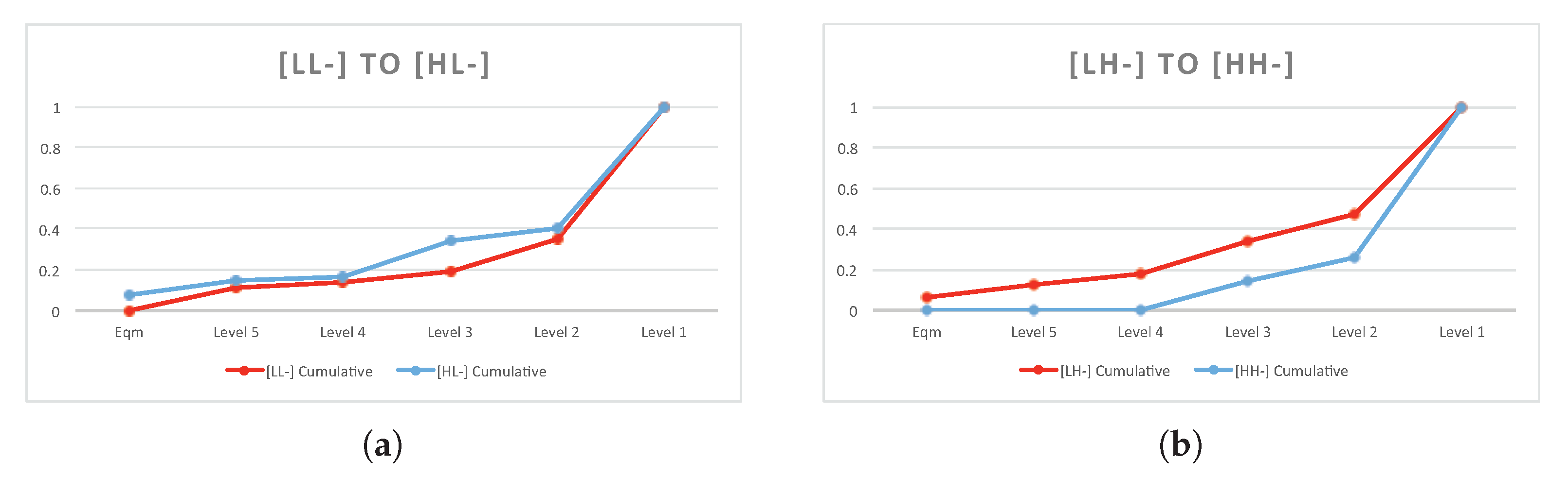
As mentioned in Section 2.2, the first testable prediction involved fixing the subject’s first- and second-order beliefs and examining the effect of the changing cost of reasoning on the subject’s behavioral levels. There were essentially two comparisons in this case: a comparison between treatment [LL-] and treatment [HL-], and between treatment [LH-] and [HH-]. Note that in both comparisons, the cost of reasoning for the subject varied from low to high; therefore, it was crucial to have partial revelation of the subject’s (role A) memorization task. In the partial revelation treatment, role B (the opponent) only knew the probability distribution of the subject’s memorization task (0.5, 0.5; L, H); therefore, even with the subject’s own tasks varying between two treatments, the subject’s second-order belief was controlled to be the same. There were 222 pairs of comparison in total. The summary statistics of the comparisons are presented in

Table 7. The frequency of changing behavioral levels with increasing cost of reasoning.

Pair Name (From Game a to Game b)	# of Pairs	Treatment	Decreases	Constant	Increases
G16 to G9	111	LL- to HL-	20.72%	43.24%	36.03%
G7 to G14	111	LH- to HH-	39.64%	49.55%	10.81%
Combined	222	L?- to H?-	30.18%	46.40%	23.42%

. The plotted distribution of behavioral levels is presented in Figure 5. To aid with the interpretation of the results, the behavioral levels in the figure are presented in a reverse order (i.e., higher level on the left and lower level on the right).

When the opponent’s cognitive load was controlled to be high and with partial revelation, subjects weakly decreased their behavioral levels 89.19% of the time (39.64% strict decrease). In Figure 5b, the [LH-] treatment is first-order stochastic dominant over the [HH-] treatment. The Wilcoxon test (

Table 8. Test results for equality of distribution.

Comparison Group (in Treatment)	Wilcoxon p-Values (Two-Tailed)	Wilcoxon p-Values (One-Tailed)
Changing Cost of Reasoning
LL- to HL-	$0.05{}^{**}$	0.98
LH- to HH-	$0.00{}^{***}$	$0.00{}^{***}$
Changing Opponent’s Cost of Reasoning
LL+ to LH+	$0.01{}^{***}$	$0.00{}^{***}$
HL+ to HH+	$0.00{}^{***}$	1
Changing Second Order Belief
LL+ to LL-	0.11	$0.05{}^{**}$
LH+ to LH-	$0.00{}^{***}$	0.99
HL- to HL+	0.00${}^{***}$	0.00${}^{***}$
HH- to HH+	0.00${}^{***}$	1
Against Computer (Nash)
L to H	0.00${}^{***}$	0.00${}^{***}$

${}^{*}$ indicates $<10\%$ significance, ${}^{**}$ indicates $<5\%$ significance, and ${}^{***}$ indicates $<1\%$ significance.

) was significant at the 1% level for the comparison of the distributions of behavioral levels between these two strategic environments. When regressing the behavioral level on the treatment dummy, the result (

Table 9. Regression results for treatment effects.

Comparison Group (in Treatment)	Relevant Dummy	Constant	Number of Obs.
Changing Cost of Reasoning
LL- to HL-	0.34 ${}^{*}$ (0.18)	1.78 ${}^{***}$ (0.14)	222
LH- to HH-	−0.77 ${}^{***}$ (0.16)	2.18 ${}^{***}$ (0.12)	222
Changing Opponent’s Cost of Reasoning
LL+ to LH+	−0.27 ${}^{*}$ (0.14)	2.03 ${}^{***}$ (0.11)	444
HL+ to HH+	0.33 ${}^{***}$ (0.10)	1.55 ${}^{***}$ (0.07)	444
Changing Second Order Belief
LL+ to LL-	−0.25 (0.18)	2.04 ${}^{***}$ (0.12)	333
LH+ to LH-	0.41 ${}^{***}$ (0.15)	1.77 ${}^{***}$ (0.09)	333
HL+ to HL-	0.57 ${}^{***}$ (0.15)	1.55 ${}^{***}$ (0.10)	333
HH+ to HH-	−0.48 ${}^{***}$ (0.09)	1.89 ${}^{***}$ (0.06)	333

${}^{*}$ indicates $<10\%$ significance, ${}^{**}$ indicates $<5\%$ significance, and ${}^{***}$ indicates $<1\%$ significance. Standard errors in parenthesis.

) suggested that the coefficient for treatment dummy was 0.77, which was significant at the 1% level. This implied that the estimated behavioral level weakly decreased when the subject’s own cognitive load increased when facing an opponent with high cognitive load. The finding is consistent with the EDR model. The relatively large proportion (49.55%) of constant levels may seem quite surprising at first look. One possible explanation is that these subjects may have had different cognitive bounds in the two treatments. In the [LH-] treatment, subjects may have adjusted their behavioral levels downward from their cognitive bound in that treatment due to some belief they formed when facing opponents with high cognitive loads. In the [HH-] treatment, subjects who had a lower cognitive bound (as they had a high cognitive load) may have displayed a lower behavioral level. When the two behavioral levels from two treatments coincided, I observed no changes in the behavioral levels in the treatment comparison.

The result for the comparison between [LL-] and [HL-] is less clear. As shown in Table 7, 63.97% of the comparisons had weakly decreasing behavioral levels (20.72% strict decrease), and a noticeable percentage (36.03%) of the comparisons had increasing levels. The Wilcoxon test statistic rejected the null hypothesis that the two strategic environments have the same distribution of behavioral levels at the 5% level. However, upon further checking using a one-tail Wilcoxon test, the distribution of behavioral levels shifted rightward when cognitive load changed from low to high when facing an opponent with a low cognitive load. When conducting the standard GLS random effect regression, the coefficient on the treatment dummy was positive and significant at the 10% level.

In this analysis, I treated equilibrium level as the highest level, since it requires the subjects to perform multiple steps of iterative best responses. However, since many games have equilibrium at the boundary of the limit interval (games 2, 4, 6, 10, 15, and 16 have the equilibrium at the lower limit; games 3, 5, 8, and 12 have the equilibrium at the upper limit), if the subject chooses an equilibrium action by naïvely playing at the boundary, then this behavioral level should not be considered as a higher level than any of the k levels. This was not the case for this comparison pair. Although game 9 ([HL-]) had 7.21% equilibrium guesses, those guesses were not at the boundary. However, upon further checking of games 16 ([LL-]) and 9 ([HL-]), I found that the level-5 type in game 16 had the same strategy as the equilibrium strategy of that game. Therefore, some of the equilibrium strategies in game 16 were pooled into level-5 type, which may be one possible explanation for the significant positive coefficient on the treatment dummy. Another explanation may be that the subjects felt more motivated to reason at higher strategic levels when they saw the opponents had easier strategic environments (memorizing three letters) as opposed to their own difficult strategic environments (memorizing seven letters). As a result, they displayed higher behavioral levels. This explanation suggests that other factors, such as motivation factor, may also play a role in determining a subject’s behavioral levels.

5.4. Result 2: Increasing Cost of Reasoning for Opponent

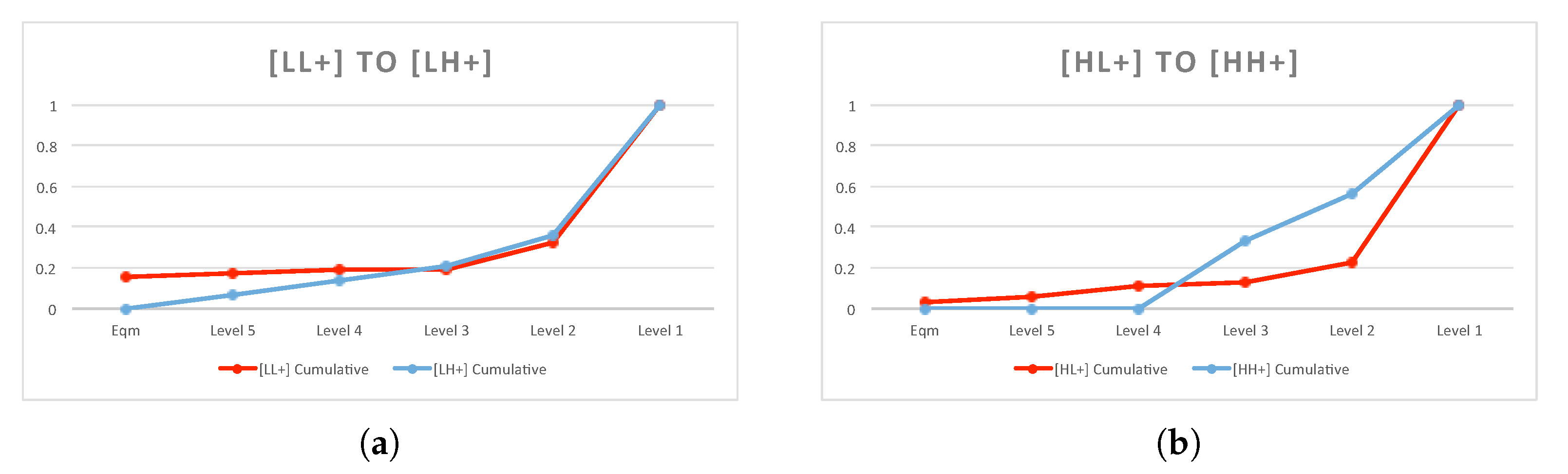
To examine the effect of changing the first-order belief on a subject’s behavioral level in games, I selected pairs of games with changing cognitive loads for the opponents. For example, a comparison of behavioral levels for games 1 and 4 served the purpose. In game 1 ([LL+]), player 1 has a low cognitive load when facing an opponent with a low cognitive load, and there is full revelation of each other’s strategic environment. In game 4 ([LH+]), player 1 has a low cognitive load when facing an opponent with high cognitive load, and again, there is full revelation of the treatments. I found 444 pairs of comparison for the cases wherein the subjects had low cognitive loads, and another 444 pairs of comparison for the cases when they had high cognitive loads. The detailed comparison groups and summary statistics are shown in

Table 10. The frequency of changing behavioral levels with increasing cost of reasoning for opponent.

Pair Name (From Game a to Game b)	# of Pairs	Treatment	Decreases	Constant	Increases
(G1, G8) to (G4, G15)	444	LL+ to LH+	23.87%	55.86%	20.27%
(G6, G13) to (G3, G12)	444	HL+ to HH+	15.54%	41.44%	43.02%
Combined	888	?L+ to ?H+	19.71%	48.65%	31.64%

. The plotted distribution of behavioral levels is presented in Figure 6.

The combined results were the opposite of the theory prediction, with a significant 31.64% of cases of increasing behavioral levels. However, upon further checking, the majority of the increasing cases occurred when subjects are having high cognitive load. When subjects had low cognitive load, 79.73% of the time, they weakly decreased their behavioral levels when their opponents’ cognitive loads changed from low to high (23.87% strict decrease). Figure 6a illustrates that [LL+] games had more guesses at higher levels. This result is consistent with the EDR model. When a subject’s cost and second-order belief was controlled across the two strategic environments, he was responsive to the changes in his opponent’s cost of reasoning. However, some of these adjustments in behavioral levels were not strictly decreasing. If the subject believed that the increased opponent’s cost of reasoning was not large enough to decrease the opponent’s behavioral level by one, the subject’s behavioral level remained the same across the two strategic environments. This partially explains the high percentage (55.86% and 41.44%) of constant behavioral levels in Table 10. When the subject had a high cognitive load and his opponent’s cognitive load changed, the result did not comply with the EDR model. A total of 43.02% of the pairs showed increasing behavioral levels across the two strategic environments. The frequency of levels in Table 6 reveals that most subjects had level 1 guesses in games 6 (83.78%) and 13 (70.27%). This gave subjects much less room to adjust their behavioral levels downward compared to another strategic situation. Any behavioral level that was beyond level 1 in games 3 and 12 was considered as moving the behavioral level upward. This was one major limitation in observing the effects of changing the first-order belief when the subject had a high cost of reasoning (i.e., high cognitive load).

The Wilcoxon signed-rank test rejected the null hypothesis that the level distribution was the same for both treatment comparisons ([LL+] to [LH+] and [HL+] to [HH+]). However, the one-tail test suggested that when the subject had low cognitive load, increasing his opponent’s cost of reasoning shifted the former’s level to the left (to lower levels, significant at the 1% level). However, when the subject had high cognitive load, the level distribution shifted to the right. The regression coefficients suggested that increasing the opponent’s cost of reasoning decreased the behavioral level when the subject had a low cognitive load (significant at the 10% level).

5.5. Result 3: Changing the Second-Order Belief

In the experiment, I used a (0.5, 0.5) probability distribution on the revelation of cognitive load treatments to control for the subject’s second-order belief. In the full revelation treatment, role B knew the exact memorization task that was received by role A (the subject), either three (low load) or seven letters (high load) with a probability of one. Therefore, role A’s (the subject) second-order belief was either ((1, 0); (L, H)) or ((0, 1); (L, H)). In the partial revelation treatment, role B knew that the probability of three or seven letters for role A was (0.5, 0.5), which made role A (the subject) have a second-order belief of ((0.5, 0.5); (L, H)). If comparing two games with different second-order beliefs for the subject, with everything else controlled as constant, then a second-order belief of low load with probability of one should be considered as more cognitively capable perceived by role B than a second-order belief of((0.5, 0.5); (L, H). The experiment, as shown in

Table 11. Subject’s belief about his opponent’s cognitive load.

		Belief Elicitation
		3 Letters	7 Letters	Not Sure	Sum
	3 Letters	591	51	24	666
Treatments	7 Letters	97	546	23	666
	(0.5 L, 0.5 H)	143	111	190	444

, supported that most subjects had a clear understanding of their opponent’s cognitive load when the load was explicitly elicited, and they almost had uniform beliefs about their opponents’ cognitive loads when they were in the partial revelation treatment as role B.

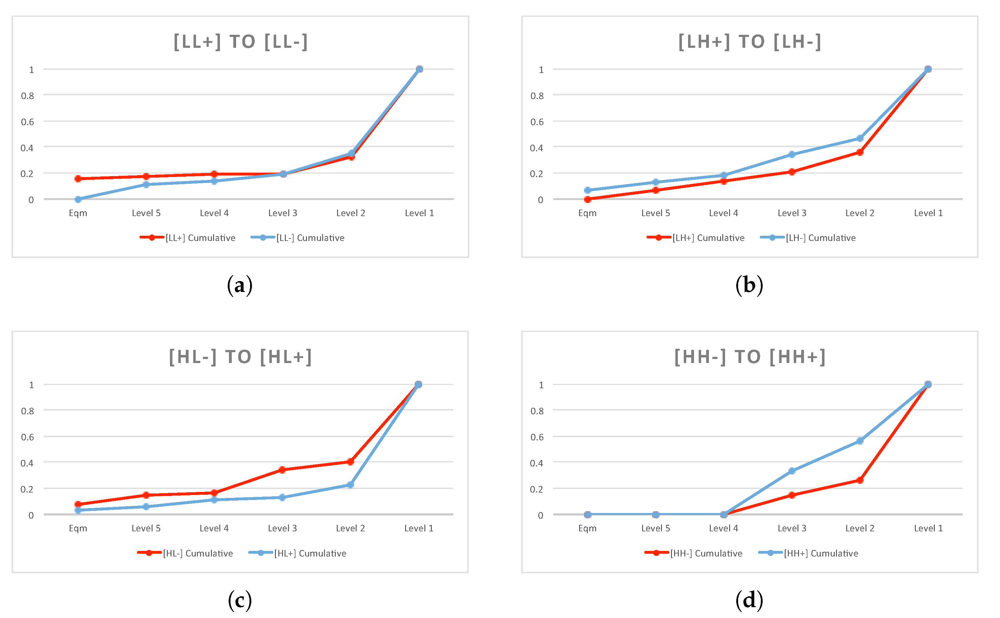
In the dataset, I found 888 pairs for comparison that allowed me to examine the effect of changing the second-order belief. I separated them into two groups: a comparison between the full revelation of low load to partial revelation, and a comparison between a partial revelation and a full revelation of high load. Both comparisons were performed in the direction of increasing second-order belief (i.e., $c_i^{ij}$ increases). The detailed comparison pairs and summary statistics are listed in

Table 12. The frequency of changing levels with changing second-order belief.

Pair Name (From Game a to Game b)	# of Pairs	Treatment	Decreases	Constant	Increases
Second order belief: Low to (0.5 Low, 0.5 High)
(G1, G8) to G16	222	LL+ to LL-	25.68%	51.35%	22.97%
(G4, G15) to G7	222	LH+ to LH-	20.27%	43.69%	36.04%
Combined	444	L?+ to L?-	22.97%	47.52%	29.50%
Second order belief: (0.5 Low, 0.5 High) to High
G9 to (G6, G13)	222	HL- to HL+	35.14%	52.70%	12.16%
G14 to (G3, G12)	222	HH- to HH+	14.86%	45.50%	39.64%
Combined	444	H?- to H?+	25.00%	49.10%	25.90%

. The distribution of behavioral levels is plotted in Figure 7.

The effect of changing the second-order belief was generally weak, except for the cases where the subjects had high cognitive loads when facing opponents with low cognitive loads. For the treatment where both players had low cognitive loads, about 77.03% of the pairs had weakly decreasing behavioral levels when second-order belief changed from full to partial revelation. Among these comparisons, only 25.68% had strictly decreasing levels. This finding suggested that the changes in second-order belief may not have been strong enough for the subjects to adjust their behavioral level downward, even though both subjects had a low cognitive load and were relatively competent at contemplating over the strategic environment. To examine the effect of the second-order belief, it was first necessary to determine the effect of changing the first-order belief for the same group of subjects. In Table 10, the subject’s behavioral responses to the changing opponent’s cognitive load were limited when the subject had a high cognitive load. Now, consider the finding in the [LH+] to [LH-] comparison to the [HH-] to [HH+] comparison (Table 12); changing the second-order belief of the subject effectively changed his opponent’s first-order belief. If the subject holds the belief about his opponent (who has a high cognitive load treatment) that the changes in his opponent’s behavioral level are limited, then the subject should not decrease his behavioral level at all. This partially explains the low frequency of strictly decreasing behavioral levels for subjects who faced opponents with high cognitive loads.

The comparison between [HL-] and [HL+] is consistent with the EDR model. In Figure 7c, the [HL-] treatment is first-order stochastic dominant over the [HL+] treatment. Of the guesses, 87.84% had weakly decreasing behavioral levels, with 35.14% having strict decreases. Changing from partial revelation to full revelation of high cognitive load, the second-order belief decreased the subject’s cognitive capability perceived by their opponent. Subjects were responsive to this change in the belief system, and adjusted their behavioral levels downward to best respond to their opponents. Testable prediction 3 suggests that if the subject’s behavioral level is binding by their cognitive bound, then they are not able to make further adjustments according to their changing beliefs. The large percentage of constant levels for these comparisons supported this statement.

The Wilcoxon test results showed that the level distribution changed for changing second-order belief. When conducting a one-tailed test, the test result suggested that for [LH+ to LH-] and [HH- to HH+] treatments, the distribution of levels significantly (at the 1% level) shifted rightward (increasing behavioral levels). This may have occurred due to the subject’s belief that their opponent with high cognitive load will engage in higher behavioral level. This result seems to comply with the results in Section 5.4, but the underlying reasons need further investigation.

The regression coefficient on the treatment dummy further supported the results. Since the treatment dummy was coded as zero with full revelation and one with partial revelation, the coefficient of 0.57 for [HL-, HL+] comparison suggested that the behavioral level decreased from partial to full revelation. It was significant at the 1% level. Again, the [LH+, LH-] and [HH-, HH+] comparisons were the opposite direction of model predictions, and they were also highly significant. In general, when the subjects faced opponents with high cognitive loads, they were responsive to changing second-order beliefs, but not in the direction that is predicted by the EDR model. However, when they faced more cognitively capable opponents, then they were mostly responsive to this change in the belief system because they thought their opponents were responsive to this information in their strategic environment. This finding is consistent with the EDR model when the opponent has a low cognitive load, which supports the opposite direction when the opponent is in a less cognitively capable situation.

5.6. Result 4: Cognitive Bound

In block 2 of the experiment, the subjects played against the computer. They were told that the computer was playing a Nash equilibrium strategy, and the equilibrium concept was explained. However, they were not taught the method to derive the equilibrium. The behavioral levels from the guesses in these two games should be considered as the highest levels they could achieve under each cognitive load treatment. I selected all the games with the same cognitive load treatment, either low cognitive load or high cognitive load, and pooled the results. A pairwise comparison between the pooled data and behavioral level obtained from games 17 and 18 allowed me to examine the existence of cognitive bounds. There were 888 pairs of comparison for each type of cognitive load, and the summary statistics are shown in

Table 13. The frequency of changing behavioral levels comparing to cognitive bound.

Cognitive Bound	# of Pairs	Decreases	Constant	Increases
Low cognitive bound
(G1, G2, G4, G7, G8, G11, G15, G16) to G17	888	18.36%	33.45%	48.20%
High cognitive bound
(G3, G5, G6, G9, G10, G12, G13, G14) to G18	888	21.96%	48.20%	29.84%
Combined	1776	20.16%	40.82%	39.02%

.

The result for low cognitive load treatment was interesting: 48.20% of the guesses from block 1 games had behavioral levels lower than the subject’s respective cognitive bound (level in game 17). Less than 20% of guesses had higher behavioral levels. This suggested that in many block 1 games, subjects purposely adjusted their behavioral levels downward due to different strategic situations, even though they had reached higher levels. For high cognitive load treatment, about 30% of behavioral levels increased from block 1 games to game 18. However, about 50% of the guesses had the same behavioral level across the two situations. Since high cognitive load inherently restricts the subject’s cognitive ability, there may have been less room for downward adjustments for block 1 games. Due to the large percentage of weakly increasing levels from block 1 to block 2 games, I concluded that cognitive bound existed in most cases. In some situations, cognitive bound was strictly higher than the subject’s behavioral levels in games. In some situations, cognitive bound was the same as the behavioral levels. Such cases were largely observed in the high cognitive load treatment.

To examine whether high cognitive load had a lower level distribution, I conducted a Wilcoxon signed-rank test on the estimated behavioral levels of games 17 (low load) and 18 (high load). Table 8 shows that the distributions of levels for the two treatments were significantly different at the 1% level. The one-tailed test indicated that the distribution of low load cognitive bound levels was to the right of the distribution of high load cognitive bound levels. This finding indicated that subjects had a higher cognitive bound when receiving low cognitive load treatment (memorizing a string of three letters) compared to receiving a high cognitive load treatment (memorizing a string of seven letters).

5.7. Robustness Check

During the guessing games, subjects needed to memorize a string of three or seven letters and recall the letters after they finished the guessing game. In this subsection, I present the results of this memorization task. Although the subjects were fully aware that if they failed to recall all the letters correctly, they would earn zero points for that round of the game, there were still some cases of wrong recalls due to reasons such as lack of attention or being too focused on the guessing game. I wanted to control the experimental results for such cases, as the subjects may have engaged in reasoning at higher levels when cognitive load did not fully apply.

Table 14. Results of the memorization task.

	3 Letters ${}^{***}$ (Low Load)	7 Letters (High Load)	Total
Correct	97.30%	90.89%	94.09%
Wrong	2.70%	9.11%	5.91%
# of tasks	999	999	1998

^* indicates $<10\%$ significance, ${}^{**}$ indicates $<5\%$ significance, and ${}^{***}$ indicates $<1\%$ significance.

shows the results of the memorization tasks. Most of the memorization tasks were perfectly performed. Not surprisingly, low cognitive load (three-letter memorization task) had more correct recalls, about 7% more than the high cognitive load task. The difference was significant at the 1% level.

To check whether poor performance of the memorization task affected the treatment results, I excluded the data with wrong recalls and performed the analysis again. The comparison pair was dropped from the sample if either game of the pair had incorrect recalls. This was performed to ensure that the cognitive load was fully in effect, so that high cognitive load added difficulties to thinking through the guessing games at higher levels, and the cost of reasoning was higher.

Table 15. Summary of the robust results with incorrect recalls dropped.

Pair Name (From Game a to Game b)	# of Pairs	Treatment	Decreases	Constant	Increases
Increasing Cost of Reasoning
G16 to G9	107	LL- to HL-	20.56%	43.93%	35.51%
G7 to G14	77	LH- to HH-	40.26%	48.05%	11.69%
Combined	184	L?- to H?-	28.80%	45.65%	25.54%
Increasing Cost of Reasoning for Opponent
(G1, G8) to (G4, G15)	426	LL+ to LH+	23.71%	56.10%	20.19%
(G6, G13) to (G3, G12)	392	HL+ to HH+	16.33%	42.09%	41.58%
Combined	818	?L+ to ?H+	20.17%	49.39%	30.44%
Second order belief: Low to (0.5 Low, 0.5 High)
(G1, G8) to G16	214	LL+ to LL-	26.17%	50.93%	22.90%
(G4, G15) to G7	211	LH+ to LH-	21.33%	44.08%	34.60%
Combined	425	L?+ to L?-	23.76%	47.53%	28.71%
Second order belief: (0.5 Low, 0.5 High) to High
G9 to (G6, G13)	202	HL- to HL+	35.64%	52.48%	11.88%
G14 to (G3, G12)	152	HH- to HH+	15.13%	45.39%	39.47%
Combined	354	H?- to H?+	26.84%	49.44%	23.73%

presents the treatment results after the robustness check. Treatments that involved high cognitive load had more data points dropped. For example, the [HH-] to [HH+] comparison had 444 pairs of comparison in the original sample. After robustness check, about 100 pairs were dropped. However, the results did not change much compared to the results presented in results 1 to 3 (Section 5.3, Section 5.4 and Section 5.5). The changes were mostly within 1%. I can therefore safely conclude that the original results were robust. The quality of the memorization task (i.e., whether the letters were correctly recalled) was almost independent of the treatment effects. Even in the cases of wrong recalls, the effect of cognitive load still applied to the subjects.

5.8. Cognitive Tests

In this subsection, I examine the results of the Mensa practice test. The test is composed of 10 questions and has a time limit of 10 min. Some subjects finished earlier, but they could never run overtime. Each correct answer is worth 1 point and all the unattempted questions are marked as 0 points. The score distribution of 104 subjects (seven missing) is presented in

Table 16. Summary statistics of cognitive test score and the counts of level changes following theory predictions.

	(1)	(2)	(3)	(4)	(5)	(6)
	Test Score	Sum.Strict	Sum.Weak	Cost.Weak	1st.Weak	2nd.Weak
Points possible	10	18	18	2	8	8
Max	10	13	18	2	8	8
Min	2	0	7	0	2	1
Median	7	4	13	2	6	6
Mean	7	4	13	1.5	5.5	6

. There are a few very low points (2 or 3), and six subjects had scores of 10. Most subjects earned seven or eight points in this test.

To examine whether there are heterogeneous treatment effects in this experiment due to exogenous cognitive ability, I first determined a measure of the treatment effect. Out of all the results discussed in results 1 to 3 (Section 5.3, Section 5.4 and Section 5.5), there are in total 18 pairs of comparison. For each subject, I recorded one for the pair if the level change followed the theory prediction, and zero otherwise. As listed in Table 16, column Sum.Strict includes all the 18 comparisons, and only strict changes of levels are recognized. For example, if the pair game 16–game 9 had level 2 in both games, it is coded zero under Sum.Strict. However, column Sum.Weak allows weak changes; therefore, the above-mentioned scenario is coded as one under this column. The EDR model mostly discusses weak behavioral level changes because, in some cases, the changes in belief system or costs are not big enough to shift a behavioral level downwards by one level (evidenced by a large percentage of constant levels). Due to this reason, I considered “weak” changes, and decomposed them into columns (4) to (6), which cover the three main results. When limited to strict changes, a number of subjects had zero pairs following theory prediction (10 out of 111 subjects), and most subjects had only three or four pairs that had changes that could be predicted by the EDR model. However, when allowing weak changes, seven subjects had all the comparison pairs that were theory-predicted directional level changes, and most subjects had about 13 to 14 comparisons that could be predicted by the EDR model. The last three columns in Table 16 present results for each treatment separately.

To test whether cognitive ability had any correlation with the treatment effects, I ran a regression after dropping the subjects with missing test scores. The result is presented in

Table 17. Regression results for cognitive test scores on correct directional changes of behavioral levels in block 1 games.

	Sum.Strict	Sum.Weak	Cost.Weak	First Order.Weak	Second Order.Weak
Test Score	0.03 (0.16)	0.36 ${}^{**}$ (0.18)	−0.04 (0.04)	0.23 ${}^{**}$ (0.11)	0.17 ${}^{*}$ (0.10)
Gender (F)	−0.73 (0.57)	1.43 ${}^{**}$ (0.60)	0.03 (0.13)	0.83 ${}^{**}$ (0.37)	0.57 ${}^{*}$ (0.34)
Class Standing	0.33 (0.24)	−0.18 (0.25)	−0.01 (0.05)	−0.13 (0.15)	−0.04 (0.14)
Major	−0.02 (0.12)	0.00 (0.13)	−0.03 (0.03)	−0.03 (0.08)	0.01 (0.07)
Constant	3.09 ${}^{*}$ (1.67)	10.04 ${}^{***}$ (1.75)	1.76 ${}^{***}$ (0.37)	3.94 ${}^{***}$ (1.08)	4.34 ${}^{***}$ (1.00)
# of Obs.	104	104	104	104	104

“Weak” includes constant levels and decreasing levels, while “strict” only includes strictly decreasing levels. ${}^{*}$ indicates $<10\%$ significance, ${}^{**}$ indicates $<5\%$ significance, and ${}^{***}$ indicates $<1\%$ significance. Standard errors in parenthesis.

. I used gender, class standing, and major as control variables. This information was collected at the end of the experiment. It appears that the cognitive test score and the female dummy variable were positively correlated with weak changes (at a 5% significance level), and the treatments changing the opponent’s cost of reasoning (changing first-order belief) and changing second-order belief. The results showed some heterogeneous treatment effects in which the more cognitively capable subjects were more responsive to the treatments as predicted by the EDR model, especially in those requiring adjustments in response to the changing strategic environment of their opponents. When the strategic environment changed, these subjects were more likely to actively adjust their actions to gain possible strategic advantages.

Since the result above suggested that more cognitively capable subjects’ responses to changing strategic environment were more coherent with the EDR model, I separated the subjects into two groups according to cognitive test scores. Subjects with scores of eight or above were labeled as high cognitive subjects (high), and the remainder were labeled as low cognitive subjects (low).

Table 18. Results 1 to 3 separated by cognitive test scores.

			Changes in Behavioral Levels
Treatment	Cog Test	# of Pairs	Decreases	Constant	Increases
Result 1: Increasing Cost of Reasoning
LL- to HL-	High	45	22.22%	37.78%	40.00%
LL- to HL-	Low	59	16.95%	47.46%	35.59%
LH- to HH-	High	45	28.89%	55.56%	15.56%
LH- to HH-	Low	59	35.59%	57.63%	6.78%
Result 2: Increasing Cost of Reasoning for Opponent
LL+ to LH+	High	180	19.44%	59.44%	21.11%
LL+ to LH+	Low	236	27.54%	53.39%	19.07%
HL+ to HH+	High	180	20.00%	47.22%	32.78%
HL+ to HH+	Low	236	12.29%	36.44%	51.27%
Result 3.1: Second order belief: Low to (0.5 Low, 0.5 High)
LL+ to LL-	High	90	23.33%	53.33%	23.33%
LL+ to LL-	Low	118	28.81%	50.85%	20.34%
LH+ to LH-	High	90	20.00%	44.44%	35.56%
LH+ to LH-	Low	118	19.49%	42.37%	38.14%
Result 3.2: Second order belief: (0.5 Low, 0.5 High) to High
HL- to HL+	High	90	35.56%	48.89%	15.56%
HL- to HL+	High	118	34.75%	55.08%	10.17%
HH- to HH+	High	90	21.11%	50.00%	28.89%
HH- to HH+	High	118	11.02%	40.68%	48.31%

presents results 1–3 again, separated by the cognitive test scores. As discussed in results 1 to 3 (Section 5.3, Section 5.4 and Section 5.5), I found significant asymmetries arising from the different strategic environments. Separating the subjects into two groups according to cognitive test scores allowed a closer examination of the source of the asymmetry. In Table 18, result 2 and result 3.1 highlight the relatively stable performance for the high cognitive subjects. As discussed in Section 5.4, subjects’ responses to their opponents’ changing cost of reasoning depended on their own cost of reasoning. In general, their adjustments in behavioral levels only followed the EDR model when they had a low cost of reasoning. This observation is untrue for the high cognitive subjects, who showed relatively stable performance regardless of their own strategic environment, with about 20% of the comparisons strictly following the EDR model. I observed a slight increase of 10% for those that did not follow the model; however, in general, the performance did not vary considerably. For the low cognitive subjects, the difference was huge. The 27.54% for comparison pairs that strictly followed the model decreased to 12.29%, and, more strikingly, the percentage of pairs that did not follow the model increased from 19.07% to 51.27%. This huge difference showed that the asymmetry found in the previous results was mostly due to these low cognitive subjects. There was a similar observation for result 3.1, where the high cognitive subjects had relatively stable performance regardless of their opponents’ cognitive loads, whereas the low cognitive test score subjects were very sensitive to their opponents’ strategic environments. Therefore, I concluded that the majority of asymmetric results found in results 2 and 3.1 were primarily driven by the low cognitive subjects. They were responsive to the treatments under the condition that they were in a more cognitively advanced situation. For results 1 and 3.2, both high and low cognitive subjects responded asymmetrically toward the treatment. However, as evidenced in Table 18, the changes from the low cognitive group were much greater than those of their counterparts.

The impact of cognitive ability on treatment effects was further evidenced by the regression results. In

Table 19. Regression results for treatment effects and cognitive test scores on behavioral levels.

Comparison	Dummy	Score	Dummy * Score	# Obs.
Changing Cost of Reasoning
LL- to HL-	0.81 (0.79)	0.07 (0.07)	−0.06 (0.11)	208
LH- to HH-	−2.13 ${}^{***}$ (0.73)	−0.11 (0.10)	0.19 ${}^{*}$ (0.10)	208
Changing Opponent’s Cost of Reasoning
LL+ to LH+	−1.15 (0.77)	−0.04 (0.09)	0.12 (0.10)	416
HL+ to HH+	1.67 ${}^{***}$ (0.44)	0.08 (0.05)	−0.19 ${}^{***}$ (0.06)	416
Changing Second Order Belief
LL+ to LL-	−1.06 (0.75)	−0.04 (0.09)	0.11 (0.10)	312
LH+ to LH-	1.77 ${}^{**}$ (0.80)	0.08 (0.05)	−0.19 ${}^{*}$ (0.11)	312
HL+ to HL-	1.08 (0.75)	0.08 (0.05)	−0.07 (0.10)	312
HH+ to HH-	−1.85 ${}^{***}$ (0.37)	−0.11 ${}^{***}$ (0.04)	0.19 ${}^{***}$ (0.05)	312

${}^{*}$ indicates $<10\%$ significance, ${}^{**}$ indicates $<5\%$ significance, and ${}^{***}$ indicates $<1\%$ significance. Clustered individual standard errors in parenthesis.

, the interaction term is significant for the comparison pairs that did not follow the EDR model ([HL+ to HH+], [LH+ to LH-], and [HH+ to HH-]). This implied that higher cognitive test scores skewed the effects of the treatment in the direction pointed by the EDR model. It seems that cognitive ability plays an important role for the subjects to display behavioral changes that can be predicted by the EDR model. The cognitive ability was captured endogenously by the treatment design in this experiment with two kinds of cognitive load. As discussed previously, the results differed systematically according to the amount of cognitive resources. Cognitive ability was also captured exogenously by the Mensa practice test, as discussed in this section. Within the asymmetric findings, subjects with higher cognitive test scores had more stable performance regardless of their own cognitive load, and were generally more predictable by the EDR model.

6. Concluding Remarks

In this study, I designed a laboratory experiment to examine the consistency of players’ strategic sophistication formulated by the level-k model. Following the endogenous depth of reasoning framework, I controlled the strategic environment by varying the cost of reasoning for the subjects, and their first- and second-order beliefs about their opponents.

My findings were consistent with the EDR model under some conditions. When the strategic environment was carefully controlled, subjects were very responsive towards the changes in the environment. Subjects who have more cognitive resources (in a low cognitive load treatment) or subjects who are facing opponents with less cognitive resources (in a high cognitive load treatment) change strategies systematically. This behavior can be predicted by the EDR model. Subjects in a strategically disadvantaged situation (high cognitive load treatment) have less room for strategic adjustments. In some of my findings, subjects appeared to try to achieve higher behavioral levels when they were under the high cognitive load treatment. The reason for this is still unclear. It may due to the awareness of the strategic disadvantage and the extra effort of the subjects under such situations, or some other behavioral factors existed that were not captured by the EDR model. The underlying reason needs further investigation. The effect of cognitive ability on the treatments was also captured by the cognitive test. Subjects with higher test scores were more predictable by the EDR model, regardless of the strategic environment. This finding is in line with the asymmetry observed in my results. As the source of asymmetry was mainly the amount of cognitive resources, it is not surprising that subjects with higher cognitive test scores adjusted better in these tasks.

A level of cognitive bound existed for subjects in different strategic situations. When playing games under the same amount of cognitive resources, subjects rarely had behavioral levels that exceeded their respective cognitive bounds for that strategic situation. Significant downward adjustments occurred from the cognitive bound in response to different strategic environments. Overall, when there is a strict control over the strategic environment, changes in k-levels across games are systematic. They can be explained by the EDR model to some extent, especially for subjects in a more cognitively advantaged situation. This study only discusses the directional changes in the levels. Further studies could examine the criteria and accuracy of such predictions.

References

- Nagel, R. Unraveling in Guessing Games: An Experimental Study. Am. Econ. Rev. 1995, 85, 1313–1326. [Google Scholar]
- Stahl, D.O.; Wilson, P.W. Experimental evidence on players’ models of other players. J. Econ. Behav. Organ. 1994, 25, 309–327. [Google Scholar] [CrossRef]
- Camerer, C.; Ho, T.; Chong, J. A cognitive hierarchy model of games. Q. J. Econ. 2004, 119, 861–898. [Google Scholar] [CrossRef] [Green Version]
- Costa-Gomes, M.; Crawford, V.P.; Broseta, B. Cognition and Behavior in Normal-Form Games: An Experimental Study. Econometrica 2001, 69, 1193–1235. [Google Scholar] [CrossRef] [Green Version]
- Ho, T.H.; Cambrer, C.; Weigelt, K. Iterated Dominance and Iterated Best Response in Experimental “p-Beauty Contests”. Am. Econ. Rev. 1998, 88, 947–969. [Google Scholar] [CrossRef]
- Bosch-Domènech, A.; Montalvo, J.G.; Nagel, R.; Satorra, A. One, two, (three), infinity, ...: Newspaper and lab beauty-contest experiments. Am. Econ. Rev. 2002, 92, 1687–1701. [Google Scholar] [CrossRef] [Green Version]
- Duffy, J.; Nagel, R. On the Robustness of Behaviour in Experimental ‘Beauty Contest’ Games. Econ. J. 1997, 107, 1684–1700. [Google Scholar] [CrossRef]
- Grosskopf, B.; Nagel, R. The two-person beauty contest. Games Econ. Behav. 2008, 62, 93–99. [Google Scholar] [CrossRef]
- Ho, T.H.; Su, X. A Dynamic Level-k Model in Sequential Games. Manag. Sci. 2013, 59, 452–469. [Google Scholar] [CrossRef] [Green Version]
- Crawford, V.P.; Iriberri, N. Level-K Auctions: Can a Nonequilibrium Model of Strategic Thinking Explain the Winner’s Curse and Overbidding in Private-Value Auctions? Econometrica 2007, 75, 1721–1770. [Google Scholar] [CrossRef] [Green Version]
- Ivanov, A.; Levin, D.; Niederle, M.; Econometrica, S.; July, N. Can Relaxation of Beliefs Rationalize the Winner’s Curse?: An Experimental Study. Econometrica 2010, 78, 1435–1452. [Google Scholar] [CrossRef]
- Crawford, V.P.V.; Costa-Gomes, M.a.; Iriberri, N. Structural Models of Nonequilibrium Strategic Thinking: Theory, Evidence, and Applications. J. Econ. Lit. 2013, 51, 5–62. [Google Scholar] [CrossRef] [Green Version]
- Alaoui, L.; Penta, A. Endogenous Depth of Reasoning. Rev. Econ. Stud. 2016, 83, 1297–1333. [Google Scholar] [CrossRef] [Green Version]
- Costa-Gomes, M.A.; Crawford, V.P. Cognition and Behavior in Two-Person Guessing Games: An Experimental Study. Am. Econ. Rev. 2006, 96, 1737–1768. [Google Scholar] [CrossRef] [Green Version]
- Arad, A.; Rubinstein, A. The 11–20 Money Request Game: A Level-k Reasoning Study. Am. Econ. Rev. 2012, 102, 3561–3573. [Google Scholar] [CrossRef] [Green Version]
- Allred, S.; Duffy, S.; Smith, J. Cognitive load and strategic sophistication. J. Econ. Behav. Organ. 2016, 125, 162–178. [Google Scholar] [CrossRef] [Green Version]
- Burnham, T.C.; Cesarini, D.; Johannesson, M.; Lichtenstein, P.; Wallace, B. Higher cognitive ability is associated with lower entries in a p-beauty contest. J. Econ. Behav. Organ. 2009, 72, 171–175. [Google Scholar] [CrossRef]
- Gill, D.; Prowse, V. Cognitive ability, character skills, and learning to play equilibrium: A level-k analysis. J. Political Econ. 2016, 124, 1619–1676. [Google Scholar] [CrossRef] [Green Version]
- Stahl, D.O.; Wilson, P.W. On Players? Models of Other Players: Theory and Experimental Evidence. Games Econ. Behav. 1995, 10, 218–254. [Google Scholar] [CrossRef]
- Fragiadakis, D.E.; Knoepfle, D.T.; Niederle, M. Who is Strategic? Technical Report. Unpublished work. 2016. [Google Scholar]
- Arad, A.; Rubinstein, A. Multi-dimensional iterative reasoning in action: The case of the Colonel Blotto game. J. Econ. Behav. Organ. 2012, 84, 571–585. [Google Scholar] [CrossRef] [Green Version]
- Georganas, S.; Healy, P.J.; Weber, R.A. On the persistence of strategic sophistication. J. Econ. Theory 2015, 159, 369–400. [Google Scholar] [CrossRef] [Green Version]
- Fischbacher, U. Z-Tree: Zurich toolbox for ready-made economic experiments. Exp. Econ. 2007, 10, 171–178. [Google Scholar] [CrossRef] [Green Version]
- Agranov, M.; Caplin, A.; Tergiman, C. Naive play and the process of choice in guessing games. J. Econ. Sci. Assoc. 2015, 1, 146–157. [Google Scholar] [CrossRef] [Green Version]
Figure 1.
Screenshot of the understanding test.
Figure 2.
Screenshot of the incentivised two-person guessing game.
Figure 3.
Distribution of exact matches.
Figure 4.
Density plot of raw guesses.
Figure 5.
Cumulative level distribution for increasing cost of reasoning.
Figure 6.
Level Distribution for increasing cost of reasoning for opponent.
Figure 7.
Level Distribution for changing second-order belief.