On Optimal Leader’s Investments Strategy in a Cyclic Model of Innovation Race with Random Inventions Times

Abstract

In this paper, we develop a new dynamic model of optimal investments in R&D and manufacturing for a technological leader competing with a large number of identical followers on the market of a technological product. The model is formulated in the form of the infinite time horizon stochastic optimization problem. The evolution of new generations of the product is treated as a Poisson-type cyclic stochastic process. The technology spillovers effect acts as a driving force of technological change. We show that the original probabilistic problem that the leader is faced with can be reduced to a deterministic one. This result makes it possible to perform analytical studies and numerical calculations. Numerical simulations and economic interpretations are presented as well.

1. Introduction

Without a doubt, R&D is one of the most important determinants of firms’ competitiveness, especially in high-tech fields. However, there are different types of R&D, and their effects on firms’ performances are also different. Innovations based on certain technological systems or dominant designs give clear patterns of continuous or cumulative technological improvements. However, when technological development reaches a certain turning point, a discontinuous innovation often occurs. Many authors define such types of technological development as technological trajectory: technology is developing along a certain trajectory, and when it saturates, a new trajectory occurs together with a shift in the corresponding scientific paradigm (see, [1,2]).

Along with this argument, innovations can be classified into two types. Innovations of the first type create new technological trajectories (radical or discontinuous innovations); innovations of the second type develop product improvements along a certain technological trajectory (incremental or continuous innovations).

The invention of the transistor, which provided the basis of the semiconductor industry, gives an example of a radical technological innovation, which created a new technological trajectory. Without a doubt, innovations of this type make the strongest impact on the markets. Nevertheless, it is important to recognize that the total outcome of small continuous innovations that follow the discontinuous one can have stronger impacts than the first radical innovation. Of course, each incremental innovation can have less of an outcome than a radical one, but often their cumulative outcome is bigger. For example, the development of high-density integrated circuits is a sequence of typical continuous innovations, which create a large market by interacting with computers and other information technology products and services.

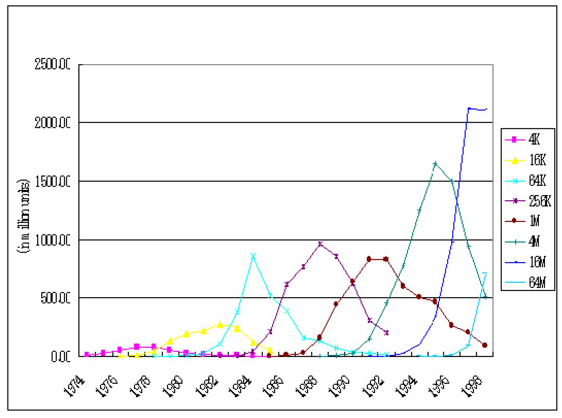
Technological developments along certain technological trajectories are mainly performed as innovation races among private companies. The regular emergences of new generations of products are observed in the industries where innovations along technological trajectories dominate. For example, transistors appeared on the market and started the new technological trajectory in the middle of the 1950s. Transistors quickly swept away vacuum tubes, which had a 100 times larger market share at that time. However, transistors themselves were swept away by integrated circuits (ICs) in the 1960s. During this process, firms severely fought with each other and this severe competition led to withdrawal of top producers of vacuum tubes from the semiconductor market. After the 1970s, Japanese firms appeared as leading producers of large-scale integrated circuits (LSIs). After the 1990s, the US firms were revived, and Korean and Taiwanese firms appeared as major players on this market. This innovation race is now continuing. Figure 1 demonstrates technological dynamics in the semiconductor industry in the period 1974–1998. In this process, the evolution of new generations of the product is driven by the innovation race among companies.

From the point of view of the innovation race, technology spillovers (including imitation) provide an important influence on industrial dynamics through each firm’s decision making. We should recognize that imitation is an important type of firms’ behavior, even in developed countries, although usually it is related mainly to the North-South problems [4].

There are various opportunities and routes for technology spillovers [5]:

(i)

Reverse-engineering of products and observation of operations;

(ii)

Spillovers from vendors of equipments or components;

(iii)

Spillovers from consultants or specialists;

(iv)

Spillovers from purchasers, which desire varieties of suppliers;

(v)

Movement of engineers to rivalry firms or spin-out;

(vi)

Analysis of patents or presentations in academic societies.

Many authors assert that imitations have negative impacts on the innovation process. Imitations erode profits of innovators, and this erosion causes a shrinking of the efforts of the innovators. Usually, the appropriability of innovations means that there is the possibility for an innovator to ensure the profit from innovations, determined by the extent of legal protection (intellectual property rights), imitation facilities, and the accessibility of complimentary assets (see [6,7]). Goto and Nagata (see [8]) assert that the early introduction of new products on the market is effective for the appropriability of innovations in high-tech fields in Japan. However, Mansfield, Schwartz and Wagner (see [9]) found that 34 new products out of 48 samples had been copied during the sample periods. They report that the average time until the sample products were imitated is about 70% of the time it took to bring the innovation to the market.

The problem of choosing the most rational type of the business strategy is an important point for firms’ managers. From the point of view of the innovation race, business strategies can be classified into two types. Strategies of the first type are the leader’s strategies, which are to firstly develop new generations of the product. Strategies of the second type are the follower’s strategies, which are to penetrate the market exploited by the leader.

The earliest release of the new generation of the product on the market is directly connected with the profitability of R&D. Particularly, in the fields where learning effects are large, the first penetrator can get the largest share of the market. However, larger R&D investment may result in shorter lifecycle of the product. It means that the return of R&D might be smaller. Smaller R&D investment allows a follower exploiting technology spillovers to get a larger share of the market. In this respect, the problem of how much resources should be allocated to R&D is an important decision-making issue for firms’ managers. Nowadays, the required R&D investments are increasing, especially in high-tech fields. The wrong decision in R&D strategy leads to bankruptcy easily.

According to Lieberman and Montgomery [10], merits of leader’s and follower’s strategies can be particularized as follows:

Merits of the leader’s strategy:

(i)

First-mover’s advantage. The innovator or first-mover can monopolize the market by using a physical lead time. The first-mover can improve the products by responding to his customers and often make a dominant design of the products. It might lead to establishing a superior brand image among the customers. The first mover can occupy rare resources;

(ii)

Learning effect. The first-mover can increase cost competitiveness by using a learning or experience effect. The experience of production of a certain product can increase efficiency of workers and improve the manufacturing process. If the first-mover constructs this kind of cost competitiveness, a follower cannot enter the market. That is why the semiconductor makers challenged to be the first-movers for new DRAM generations;

(iii)

Legal protection. The first-mover can get legal protection by intellectual property rights such as patents and copyrights. Xerox for copy machines and GE for electric bulbs dominated the market for a long time by exploiting their patents;

(iv)

Transfer cost of customers. In the case when customers should pay some cost to change their suppliers, the first-mover can take advantage (the mileage system is an example);

(v)

Network externality. If the new products or services have network externalities, the fist-mover can have an advantage over the followers. Network externality has been defined as a change in the benefit, or surplus, that an agent derives from goods when the number of other agents consuming the same kind of goods changes. As fax machines increase in popularity, for example, your fax machine becomes increasingly valuable, since you have greater use of it.

Merits of the follower’s strategy:

(i)

Free-ride of leader’s effort. Followers can freely use many things, which the first-mover built at his cost. It is difficult to exclude the use of knowledge, the outcomes of innovations, by others. In many cases, imitation is cheaper than the original innovation, although it costs more than generally expected. For example, investment in educating customers on how to use certain innovative products and infrastructure development for new products (for example, repair services) can be freely used by followers;

(ii)

Low market risk for introducing products. The first mover should take risk of uncertain innovative products and bear investments, which can eventually be found unnecessary as well as the cost of tried, and error. Followers can avoid unnecessary investments or failures by exploiting the experiences of the first mover. Actually, Japanese carmakers learn many lessons from the experience of the German carmaker Volkswagen that precedently penetrated into the US market and failed when Japanese carmakers managed to produce their cars in the US;

(iii)

Conservation of initial cost by the spillovers effect, etc. In the case of environmental changes, the first mover often faces difficulties. There are some cases where the environments on the market or technology change after the first mover commits to certain assets or processes and embarks on full-scale investments in them. In such cases, followers can get an advantage over the first mover. Because of the institutional inertia, it is difficult for the first mover to respond to environmental change, diminishing the merits of existing assets or processes and to sunk the cost of them. Ford succeeded in the passenger car market by focusing on the production of the T-type Ford. However, Ford could not respond to the preference of the customers in the differentiation of products and gave up the top position to General Motors.

Competition of innovators and the innovation race is in the focus of numerous publications (see, for instance, [11,12,13]). However, each model is focused on specific features of new product development, because this process is too complicated.

Many decision support models for corporate strategy of new product introduction are developed in marketing and operation research literature. In particular, Cohen et al. [14] carried out a multistage product development model for analyzing an optimal timing of introduction of new product to the market. Bayus [15] analyzed the competition between two companies based on the U-shaped curve between time and cost of new product development. Morgan et al. [16] extended the model of Bayus to multiple products generations. Cohen et al. [17], and Ramdas and Sawhney [18] examined the optimal line extensions from the economies of scale. Paulson Gjerde at al. [19] analyzed the optimal improvement strategy of products which had multiple features. Souza at al. [20] analyzed the optimal timing of introduction of the new product to the market with market uncertainty. These models did not address the uncertainty which is inherent in innovation.

There is also a stream of literature which is focused on theoretical studies of innovation process. Reinganum [21] introduced the game theory to analyze the leader-follower situation. Her analysis is mainly focused on the interaction between firms. She does not take into account uncertainty and assumes fixed profits. Breitmoser, Tan and Zizzo (see [22]) studied dynamic indefinite horizon R&D races with uncertainty and multiple prizes based on the Markov perfect equilibria. They presented the possibility that the stochastic R&D races framework describes real-world R&D competition. Aghion and Howitt (see [23]) are pioneers of analysis when it comes to the creative destruction situation in endogenous growth theory. Their main interest is focused on economic growth through product innovation race. Aghion et al. studied effects of competition on innovation based on the step by the step innovation game framework in the recent paper [24]. They found that competition effects positive impacts on innovation, especially in long time horizon. For a comparative analysis of different innovation process models, see the review paper [25] and the monograph [26].

In this paper, we develop a new dynamic model of optimal investments in R&D and manufacturing for a technological leader competing with a large number of identical followers. Our main goal is to develop a modeling framework which takes into account the key features of the innovation process, such as uncertainty inherent to times of inventions of a new product generations, the cyclic character of innovations, and the market competition. Although we are focused on a particular leader-follower’s case, we believe that the developed methodology can be applied to the construction of similar models which consider innovation process from different points of view.

The model is constructed according to the templates of the economic growth literature (see [27,28,29]). As in [20], our model is formulated in the form of infinite time horizon dynamic optimization problem. However, unlike the existing literature, we describe analytically the times of inventions of new generations of the product development as a Poisson-type cyclic stochastic process. The main assumption is that the probability of the development of a new generation of the product on a small time interval is proportional to the length of this interval and the innovator’s knowledge capital that is associated with accumulated innovators’ investments of some resource in R&D. Such an approach to modeling of processes with modal disturbances in dynamics is well known in the control literature (see [30]). The model is focused on the innovations along a technological trajectory. The success of this type of innovations depends mainly on the volume of R&D investments. From this point of view, we use the Poisson-type cyclic stochastic process for the modeling of evolution of the new product’s generations.

In our model, we consider the case of the development along a certain technological trajectory with a vertical products differentiation, when every innovation gives a significant improvement in the product’s quality and (or) in the level of services that the product provides (see [29]). This corresponds to the creative destruction situation when every new invention makes the previous technology obsolete. Situations of this type are widely spread in the high-tech fields.

As suggested in [31], we assume that all innovators acting on the market have two sectors: the R&D sector and the manufacturing one. All innovators make costly investments to both R&D and manufacturing. Consequently, the leader’s R&D sector develops new generations of the product and the leader’s manufacturing sector performs their production. Selling the products on the market, the technological leader obtains revenue for his R&D and manufacturing efforts. The goal of the leader is to maximize the aggregated discounted profit by optimizing both R&D and manufacturing investment policies. Concerning the technological followers, we assume that they act as imitators. When the latest generation of the product appears on the market, the product’s attributes become available for the followers. This provides followers with the ability to improve their economic performance by developing corresponding imitations (their own versions of the newest product). In this way, a technology spillovers effect is taken into account. When the followers bring their versions of the latest generation of the product onto the market, the products offer increases. As a consequence, the product’s price decreases together with the leader’s profit. This stimulates the technological leader to develop the next generation of the product. Thus, in our model, the technology spillovers effect plays the role of a driving force in the technological progress. Choosing appropriate R&D and manufacturing investment policies, the technological leader maximizes the expectation of the value of his aggregated discounted profit.

This paper is organized as follows. In Section 2, we consider a process of new product generations development performed by the technological leader and the followers. In Section 3, we describe an accepted market price formation mechanism and design the technological leader’s goal functional. In Section 4, we consider the dynamic optimization problem that the technological leader faces. We show that in the situation when the leader competes with a large number of identical followers, the original probabilistic problem can be reduced to a relatively simple deterministic one. This result makes it possible to perform analytical studies and numerical calculations. In particular, it implies the existence of optimal leader’s investments strategies and their stationarity. Numerical sensitivity analysis and economic interpretations are presented in Section 5. Section 6 presents concluding remarks.

2. Innovation Process

First, we consider the process of development of new generations of the product, performed by the technological leader.

At the initial instant of time $T_0=0$, the leader makes a decision on the amount $u\left(t\right)\equiv u_1\ge 0$ of a resource, which will be allocated to R&D. It can be leader’s labor, capital, energy or another resource, which is recognized as the determinant of the leader’s R&D activity. We assume that this amount $u\left(t\right)$ of the resource is fixed till the instant of time $T_1>T_0$, when the next generation of the product will be developed by the leader’s R&D sector. Therefore, the leader’s R&D investment policy $u\left(t\right)$ is assumed to be fixed on the time interval $[T_0, T_1]$: $u\left(t\right)\equiv u_1$ for all $t\in [T_0, T_1]$.

Starting from the instant of time $T_1$, the developed new technology is implemented in manufacturing and the leader’s research sector starts development of the next generation of the product. At the time $T_1$, the technological leader makes a decision on the amount $u\left(t\right)\equiv u_2\ge 0$ of the resource, which will be allocated to R&D. We assume that the leader’s R&D investment policy $u\left(t\right)$ is fixed till the next instant of time $T_2>T_1$, when the next generation of the product will be available, i.e., $u\left(t\right)\equiv u_2$ for all $t\in [T_1, T_2]$.

This process is repeated infinitely many times.

Thus, we have an infinite sequence of instants of time $T_0=0$, $T_{n-1}<T_n$, $n=1,2,\dots$, at which the technological leader starts the development of new generations of the product. On each n-th time interval $[T_{n-1},T_n]$, the leader’s R&D investment policy (an instantaneous amount $u\left(t\right)$ of the resource allocated to R&D) is fixed: $u\left(t\right)\equiv u_n\ge 0$ for all $t\in [T_{n-1},T_n]$.

We consider the length $l_n=T_{n-1}-T_n$ of each time interval $[T_{n-1},T_n]$, $n=1,2,\dots$, as a random variable of the Poisson type.

Let $K_n\left(t\right)$ be the leader’s knowledge capital accumulated in R&D at the instant of time $t\in [T_{n-1},T_n]$. We assume that for any $n=1,2,\dots$, we have $K_n\left(T_{n-1}\right)=0$. In our model, the current leader’s knowledge capital $K_n\left(t\right)$, $t\in [T_{n-1},T_n]$, is associated with the accumulated investment of the resource in R&D, i.e.,

$$K_n\left(t\right)=u_n(t-T_{n-1}).$$

(1)

Furthermore, $T_n$ is the instant of time when the n-th generation of the product becomes available. We assume that for any $n=1,2,\dots$, the length $l_n=T_n-T_{n-1}$ of the n-th research interval is a random variable with a smooth distribution $P_n\left(\tau \right)=P(l_n<\tau )$, $\tau >0$, satisfying the equality

$$P(l_n<\tau +\Delta \tau |l_n\ge \tau )=\rho K_n(T_{n-1}+\tau )\Delta \tau +o(\Delta \tau ),\rho >0.$$

Here ${lim}_{\Delta \tau \to 0}\frac{o(\Delta \tau )}{\Delta \tau }=0$, all lengths $l_n=T_n-T_{n-1}$, $n=1,2,\dots$, are considered as independent random variables, and $\rho >0$ is a constant parameter characterizing the efficiency of the leader’s R&D sector. Efficiency of R&D is defined as the necessary level of R&D investment to create a new innovation, namely cost efficiency.

These assumptions provide complete characterization of the random variables $l_n=T_{n-1}-T_n$, $n=1,2,\dots$, as the Poisson-type random variables (see [32] (§ 51)). Namely, the random variable $l_n=T_{n-1}-T_n$ has the following Poisson-type distribution $P_n\left(\tau \right)$ and density $p_n\left(\tau \right)=\frac{d}{dt}{P}_n\left(\tau \right)$:

$$P_n\left(\tau \right)=1-e^{-\rho u_n\frac{{\tau }^2}{2}},p_n\left(\tau \right)=\rho u_n\tau e^{-\rho u_n\frac{{\tau }^2}{2}}.$$

(2)

Consider now the process of development of new generations of the product performed by $N_f$ identical and independent technological followers.

We assume that all followers allocate equal (and fixed) amounts $u_f$ of the same resource as the technological leader to R&D on every time interval $[T_{n-1},T_n]$, $n=1,2,\dots$. Then, analogously to the case of the technological leader (see (1)), the value of each i-th follower’s knowledge capital $K_f^i\left(t\right)$, $i=1,2,\dots ,N_f$ at the instant of time $t\in [T_{n-1},T_n]$ can be represented by the following formula:

$$K_f^i\left(t\right)=u_f(t-T_{n-1}).$$

(3)

Furthermore, similarly to the case of the technological leader, we assume that the length $l_n^i$, $n=1,2,\dots$, $i=1,2,\dots ,N_f$, of the time interval needed for the i-th follower to develop its own version of the newest product is the Poisson-type random variable characterized by an efficiency parameter $\beta >0$ (which assumed to be the same for all followers) and the corresponding amount of the accumulated knowledge capital $K_f^i\left(t\right)$ (see (3)), i.e.,

$$P(l_n^i<\tau +\Delta \tau |l_n^i\ge \tau )=\beta K_f^i(T_{n-1}+\tau )\Delta \tau +o(\Delta \tau ).$$

In this case for all $i=1,2,\dots ,N_f$ and all $n=1,2,\dots$, the distribution $P^f\left(\tau \right)=P(l_n^i<\tau )$ and the corresponding density $p^f\left(\tau \right)=\frac{d}{dt}{P}^f\left(\tau \right)$ of the random variable $l_n^i$ are independent of i and n and can be represented by the following formulas (see (2)):

$$P^f\left(\tau \right)=1-e^{-\beta u_f\frac{{\tau }^2}{2}},p_f\left(\tau \right)=\beta u_f\tau e^{-\beta u_f\frac{{\tau }^2}{2}}.$$

(4)

Let $0\le N\left(t\right)\le N_f$ be the number of followers operating on the market at the instant of time $t\in [T_{n-1},T_n]$, $n=1,2,\dots$, with their versions of the latest generation of the product. As far as all followers are assumed to be independent, and the probability of the event that the i-th follower has developed its version of the newest product before time $t\in [T_{n-1},T_n]$ is equal to $P^f(t-T_{n-1})=1-e^{-\beta u_f\frac{{(t-T_{n-1})}^2}{2}}$ (see (4)) for any $M=0,1,\dots ,N_f$, we have

$$P(N\left(t\right)=M)=C_{N_f}^M{\left(1-e^{-\beta u_f\frac{{(t-T_{n-1})}^2}{2}}\right)}^M{e}^{-(N_f-M)\beta u_f\frac{{(t-T_{n-1})}^2}{2}},$$

(5)

where $C_{N_f}^M$ is the number of M-combinations of an $N_f$-set.

3. Manufacturing and Profit Maximization

This section describes the accepted market price formation mechanism and design of the technological leader’s goal functional.

Usually, in economic literature, the firm’s instantaneous production (production rate) $Y\left(t\right)$ at the instant of time $t\ge 0$ is viewed as a function of quantities of resources accumulated in manufacturing such as labor, $L\left(t\right)$, capital, $C\left(t\right)$, materials, $M\left(t\right)$, and energy, $E\left(t\right)$ (see, e.g., [27,33]):

$$Y\left(t\right)=F\left(L\right(t),C(t),M(t),E(t\left)\right).$$

In this paper, we assume that the leader’s production rate at every instant of time $t\ge 0$ is determined by the corresponding instantaneous investment $v\left(t\right)\ge 0$ of some resource. We do not concretize the nature of this resource. It can be capital, labor, energy or any other particular resource, which is invested in manufacturing. This resource can be different from the resource, which the leader allocates to R&D. In particular, we represent the leader’s production rate $Y_l\left(t\right)$ (a number of units of the product produced in the unit of time) as a function of the current investment $v\left(t\right)$ of the chosen resource as follows:

$$Y_l\left(t\right)=\sigma v^{\gamma }\left(t\right).$$

(6)

Here, $\sigma >0$ and $\gamma >0$ are the model parameters: parameter $\sigma$ characterizes the productivity level of the leader’s manufacturing sector; parameter $\gamma$ represents the leader’s marginal productivity1. In what follows. we assume that the leader’s instantaneous production rate is strictly positive (i.e., $v\left(t\right)>0$ for all $t\ge 0$).

In our model, the technological leader’s manufacturing sector produces the latest version of the product developed by its research lab. We have a sequence $T_0=0<T_1<\cdots <T_n<\dots$ of random instants of time $T_n$, $n=1,2,\dots$, at which the leader’s R&D sector develops new generations of the product. We assume that at each instant of time $T_{n-1}$, $n=1,2,\dots$, the leader makes a decision about amount $v\left(t\right)\equiv v_n>0$ of the resource which will be allocated to manufacturing on the current time interval $[T_{n-1},T_n]$2.

So, we assume that the leader’s manufacturing investment policy $v\left(t\right)$ is fixed on each time interval $[T_{n-1},T_n]$: $v\left(t\right)\equiv v_n>0$ for all $t\in [T_{n-1},T_n]$, $n=1,2,\dots$ According to (6) in this case on every time interval $[T_{n-1},T_n]$, the leader has fixed manufacturing sector’s production rate

$$Y_l\left(t\right)\equiv Y_n=\sigma v_n^{\gamma },t\in [T_{n-1}, T_n].$$

(7)

Now, we describe the accepted market price formation mechanism.

At the instant of time $t\in [T_{n-1},T_n]$, $n=1,2,\dots$, a random number $0\le N\left(t\right)\le N_f$ of followers produce their versions of the newest generation of the product. As far as all followers are supposed to be identical, each of them produces the same number

$$y_f={\sigma }_f{v}_f^{{\gamma }_f}$$

of units of the product in the unit of time. Here ${\sigma }_f>0$ and ${\gamma }_f>0$ are parameters analogous to those of the technological leader (followers’ level of productivity and marginal productivity respectively), and $v_f$ is an amount of the resource allocated by each follower to manufacturing. In this case, the current aggregated rate of total followers’ production at the instant of time $t\in [T_{n-1},T_n]$ is $Y_f\left(t\right)=N\left(t\right)y_f$. Thus (see (7)), the total supply rate of the product to the market at the instant of time $t\in [T_{n-1},T_n]$, $n=1,2,\dots$, is

$$Y\left(t\right)=Y_l\left(t\right)+Y_f\left(t\right)=\sigma v_n^{\gamma }+N\left(t\right)y_f.$$

(8)

Let $d\left(t\right)$ be the current market price of the product at the instant of time $t\in [T_{n-1},T_n]$, $n=1,2,\dots$.

Assume that the market’s demand is equal to a constant $d_0>0$ at any instant of time $t\ge 0$. Then, taking into account the equilibrium condition $d\left(t\right)Y\left(t\right)=d_0$, due to (8), we get the following formula for the current price $d\left(t\right)$ at the instant of time $t\in [T_{n-1},T_n]$:

$$d\left(t\right)=\frac{d_0}{Y\left(t\right)}=\frac{d_0}{\sigma v_n^{\gamma }+N\left(t\right)y_f}.$$

Then, due to (5) the mean value $E\left(d\right(t\left)\right)$ of the price $d\left(t\right)$ at the instant of time $t\in [T_{n-1},T_n]$, $n=1,2,\dots$, is the following:

$$E\left(d\left(t\right)\right)=\sum _{M=0}^{N_f}\frac{d_0}{\sigma v_n^{\gamma }+M{y}_f}{C}_{N_f}^M{\left(1-e^{-\beta u_f\frac{{(t-T_{n-1})}^2}{2}}\right)}^M{e}^{-(N_f-M)\beta u_f\frac{{(t-T_{n-1})}^2}{2}}.$$

(9)

Now, suppose that the leader should buy resources $u\left(t\right)$ and $v\left(t\right)$ allocated to R&D and manufacturing at prices $p_1>0$ and $p_2>0$ respectively at each instant of time $t\ge 0$. As far as the leader’s instantaneous revenue at the instant of time $t\in [T_{n-1},T_n]$ is equal to $d\left(t\right)Y_n$, the instantaneous leader’s profit $D\left(t\right)$ is represented by the formula

$$D\left(t\right)=d\left(t\right)Y_n-(p_1{u}_n+p_2{v}_n).$$

Let $\alpha >0$ be a subjective discount parameter. Then the discounted aggregated leaders profit $J_n$ on the n-th random time interval $[T_{n-1},T_n]$, $n=1,2,\dots$, can be defined as follows:

$$J_n={\int }_{T_{n-1}}^{T_n}D\left(t\right)e^{-\alpha t}dt={\int }_{T_{n-1}}^{T_n}[d\left(t\right)Y_n-(p_1{u}_n+p_2{v}_n)]e^{-\alpha t}dt.$$

Introducing the new integration variable $\tau =t-T_{n-1}$ we get

$$J_n=\prod _{i=1}^{n-1}{e}^{-\alpha l_i}·{\int }_0^{l_n}[d\left(\tau \right)Y_n-(p_1{u}_n+p_2{v}_n)]e^{-\alpha \tau }d\tau .$$

As far as all random variables $l_1,l_2,\dots ,l_n$ are independent we have

$$E\left(J_n\right)=\prod _{i=1}^{n-1}E\left(e^{-\alpha l_i}\right)·E\left({\int }_0^{l_n}[d\left(\tau \right)Y_n-(p_1{u}_n+p_2{v}_n)]e^{-\alpha \tau }d\tau \right).$$

(10)

Due to (2) the following equality takes place

$$E\left(e^{-\alpha l_i}\right)={\int }_0^{\infty }{e}^{-\alpha \tau -\rho u_i\frac{{\tau }^2}{2}}\rho u_i\tau d\tau ,i=1,2,\dots$$

Integrating the last equality by parts we get

$$E\left(e^{-\alpha l_i}\right)=1-\alpha {\int }_0^{\infty }{e}^{-\alpha \tau -\rho u_i\frac{{\tau }^2}{2}}d\tau ,i=1,2,\dots .$$

(11)

The next result gives a tool for calculation of the mean value $E\left(J_n\right)$, $n=1,2,\dots$ (see (10)).

Lemma 1.

For any $n=1,2,\dots$, the following equality takes place:

$$E\left({\int }_0^{l_n}d\left(\tau \right)e^{-\alpha \tau }d\tau \right)={\int }_0^{\infty }E\left(d\left(\tau \right)\right)e^{-\alpha \tau -\rho u_n\frac{{\tau }^2}{2}}d\tau .$$

(12)

Proof. 

For arbitrary $T>0$ and any $N=1,2,\dots$ put ${\Delta }_N^T=\frac{T}{N}$, $t_j=j{\Delta }_N^T$, $j=1,2,\dots ,N$, and consider the random process

$${\xi }_{l_n}=1\mathrm{if}{l}_n\ge \tau ,{\xi }_{l_n}=0\mathrm{if}{l}_n<\tau ,$$

and the random variable

$$J_N^T=\sum _{j=1}^{N}d\left(t_j\right)e^{-\alpha t_j}{\xi }_{l_n}\left(t_j\right){\Delta }_N^T.$$

The random variable $J_N^T$ and the random process $d\left(t\right)$ are completely characterized on the time interval $[T_{n-1}, T_n]$ by a finite number of random parameters ${\tau }_1\ge 0,\dots ,{\tau }_{N_f}\ge 0$, which are the instances of time when the corresponding followers appear on the market.

Furthermore, for any realization of ${\tau }_1,\dots ,{\tau }_{N_f}$ the corresponding realization of

$$d\left(t\right)=d_{{\tau }_1,\dots ,{\tau }_{N_f}}\left(t\right)=\frac{d_0}{\sigma v_n^{\gamma }+N\left(t\right)y_f}$$

is a piece-wise constant function with not more than $N_f$ points of discontinuity. Hence, due to the presence of the discounting factor $e^{-\alpha t}$ in the integral ${\int }_0^{l_n}d\left(\tau \right)e^{-\alpha \tau }d\tau$ for arbitrary $\epsilon >0$, there is a $T_{\epsilon }>0$, such that for any realization of random variables ${\tau }_1,\dots ,{\tau }_{N_f}$, any $T>T_{\epsilon }$ and any realization of the random variable $l_n$, we have

$$\left|{\int }_0^{l_n}d\left(\tau \right)e^{-\alpha \tau }d\tau -J_N^T\right|\le \epsilon .$$

(13)

Consider the random variable $J_N^T$ (depending on the random variables ${\tau }_1,\dots ,{\tau }_{N_f}$ and $l_n$). We have

$$E\left(J_N^T\right)=E\left(\sum _{j=1}^{N}d\left(t_j\right)e^{-\alpha t_j}{\Delta }_N^T\xi \left(l_n\right)\right)=\sum _{j=1}^{N}E\left(d\left(t_j\right)\right)e^{-\alpha t_j}E\left(\xi \left(l_n\right)\right){\Delta }_N^T.$$

As far as

$$E\left({\xi }_{l_n}\left(t_j\right)\right)=P(l_n\ge t_j)=1-P_n\left(t_j\right)=1-e^{-\rho u_n\frac{t_j^2}{2}}$$

see (2); we get

$$E\left(J_N^T\right)=\sum _{j=1}^{N}E\left(d\left(t_j\right)\right)e^{-\alpha t_j-\rho u_n\frac{t_j^2}{2}}{\Delta }_N^T.$$

Due to (9) the mean value $E\left(d\right(t\left)\right)$ is a continuous bounded function. Hence, due to (13) for arbitrary $\epsilon >0$ there is $T_{\epsilon }>0$ such that for any $T>T_{\epsilon }$ passing to a limit in the above equality as $N\to \infty$ we get

$$\left|E\left({\int }_0^{l_n}d\left(\tau \right)e^{-\alpha \tau }d\tau \right)-{\int }_0^{T}E\left(d\left(\tau \right)\right)e^{-\alpha \tau -\rho u_n\frac{{\tau }^2}{2}}d\tau \right|\le \epsilon .$$

Passing to a limit in the last inequality as $T\to \infty$, we get (12). Lemma 1 is proven. □

Due to Lemma 1 for arbitrary $n=1,2,\dots$, we get the following formula for the mean value $E\left(J_n\right)$ (see (10) and (11)):

$$E\left(J_n\right)=\prod _{i=1}^{n-1}\left(1-\alpha {\int }_0^{\infty }{e}^{-\alpha \tau -\rho u_i\frac{{\tau }^2}{2}}d\tau \right)·{\int }_0^{\infty }\left[E\left(d\left(\tau \right)\right)Y_n-(p_1{u}_n+p_2{v}_n)\right]e^{-\alpha \tau -\rho u_n\frac{{\tau }^2}{2}}d\tau .$$

(14)

Furthermore, on each time interval $[T_{n-1},T_n]$, $n=1,2,\dots$, we posit the following constraint on the leader’s investment policies3 $u_n\ge 0$ and $v_n>0$

$$E\left(J_n\right)\ge 0.$$

(15)

Here, $E\left(J_n\right)$ is the mean value (expectation) of the aggregated discounted random leader’s profit $J_n$ on the n-th time interval $[T_{n-1},T_n]$, $n=1,2,\dots$

Summarizing (14), we get the following expectation of the aggregated discounted leader’s profit on the infinite time interval $[0,\infty )$:

$$\begin{array}{cc}\hfill J& =\sum _{n=1}^{\infty }E\left(J_n\right)=\sum _{n=1}^{\infty }{\int }_{T_{n-1}}^{T_n}\left[E\left(d\left(t\right)\right)Y_n-(p_1{u}_n-p_2{v}_n)\right[e^{-\alpha t}dt\hfill \\ \hfill & =\sum _{n=1}^{\infty }\prod _{i=1}^{n-1}\left(1-\alpha {\int }_0^{\infty }{e}^{-\alpha \tau -\rho u_i\frac{{\tau }^2}{2}}d\tau \right)·{\int }_0^{\infty }\left[E\left(d\left(\tau \right)\right)Y_n-(p_1{u}_n+p_2{v}_n)\right[e^{-\alpha \tau -\rho u_n\frac{{\tau }^2}{2}}d\tau .\hfill \end{array}$$

The technological leader’s goal is to maximize the value of this functional J.

4. Dynamic Optimization Problem

The technological leader faces the following dynamic optimization problem $\left(P\right)$:

$$\begin{array}{cc}\hfill J=\sum _{n=1}^{\infty }E\left(J_n\right)=& \sum _{n=1}^{\infty }\prod _{i=1}^{n-1}\left(1-\alpha {\int }_0^{\infty }{e}^{-\alpha \tau -\rho u_i\frac{{\tau }^2}{2}}d\tau \right)\hfill \\ \hfill & ·{\int }_0^{\infty }\left[E\left(\frac{d_0\sigma v_n^{\gamma }}{\sigma v_n^{\gamma }+N\left(\tau \right)y_f}\right)-(p_1{u}_n+p_2{v}_n)\right]e^{-\alpha \tau -\rho u_n\frac{{\tau }^2}{2}}d\tau \to max.\hfill \end{array}$$

(16)

Here, quantities $u_n\ge 0$, $v_n>0$, $n=1,2,\dots$, are control parameters satisfying (15); $d_0>0$, $\alpha >0$, $\beta >0$, $\sigma >0$, $\gamma >0$, $u_f\ge 0$, $y_f={\sigma }_f{v}^{{\gamma }_f}>0$; quantities $T_0=0$, $T_{n-1}\le T_n$, $n=1,2,\dots$, are random instants of time when technological leader develops n- th generations of the product; random variables $l_n=T_n-T_{n-1}>0$, $n=1,2,\dots$, are independent and their distributions are given by the formula (see (2))

$$p_n\left(\tau \right)=\rho u_n\tau e^{-\rho u_n\frac{{\tau }^2}{2}}.$$

Furthermore, $0\le N\left(t\right)\le N_f$ is a random number of identical followers operating on the market at the instant of time $t\ge 0$; $N_f$ is a total number of followers and the distribution of $N\left(t\right)$ is given by (5).

Let us introduce auxiliary functions $\mu \left(u\right)$ on $[0,\infty )$ and $\eta (u,v)$ on $[0,\infty )\times [0,\infty )$ as follows:

$$\mu \left(u\right)=1-\alpha {\int }_0^{\infty }{e}^{-\alpha \tau -\rho u\frac{{\tau }^2}{2}}d\tau \mathrm{for}\mathrm{all}u\ge 0;$$

$$\eta (u,v)={\int }_0^{\infty }\left[E\left(\frac{d_0\sigma v^{\gamma }}{\sigma v^{\gamma }+N\left(\tau \right)y_f}\right)-(p_{1}u+p_{2}v)\right]e^{-\alpha \tau -\rho u\frac{{\tau }^2}{2}}d\tau \mathrm{for}\mathrm{all}u\ge 0,v>0;$$

$$\eta (u,0)=-p_{1}u{\int }_0^{\infty }{e}^{-\alpha \tau -\rho u\frac{{\tau }^2}{2}}d\tau \mathrm{for}\mathrm{all}u\ge 0.$$

Obviously, the function $\eta (u,v)$ is bounded on $[0,\infty )\times [0,\infty )$ and for all $u\ge 0$ the function $\mu \left(u\right)$ satisfies the inequality

$$0\le \mu \left(u\right)<1.$$

Furthermore, due to the constraint $E\left(J_n\right)\ge 0$, $n=1,2,\dots$, (see (15)), all quantities $u_n$ and $v_n$ satisfy the inequalities $u_n\le \frac{d_0}{p_1}$ and $v_n\le \frac{d_0}{p_2}$ respectively. Hence,

$$\underset{u\in [0,\frac{d_0}{p_1}]}{max}\mu \left(u\right)=\mu \left(\frac{d_0}{p_1}\right)=1-\alpha {\int }_0^{\infty }{e}^{-\alpha \tau -\rho \frac{d_0}{p_1}\frac{{\tau }^2}{2}}d\tau <1.$$

Thus, the row representing functional J (see (16)) converges absolutely and we can group its summands in an arbitrary way:

$$\begin{array}{cc}\hfill J& =\sum _{n=1}^{\infty }E\left(J_n\right)=\sum _{n=1}^{\infty }\left(\eta (u_n,v_n)\prod _{i=1}^{n-1}\mu \left(u_i\right)\right)\hfill \\ \hfill & =\eta (u_1,v_1)+\eta (u_2,v_2)\mu \left(u_1\right)+\eta (u_3,v_3)\mu \left(u_1\right)\mu \left(u_2\right)+\dots +\eta (u_n,v_n)\mu \left(u_1\right)\dots \mu \left(u_{n-1}\right)+\dots \hfill \\ \hfill & =\eta (u_1,v_1)+\mu \left(u_1\right)\left(\eta (u_2,v_2)+\mu \left(u_2\right)\left(\eta (u_3,v_3)+\mu \left(u_3\right)\left(\dots \right)\right)\right).\hfill \end{array}$$

The last equality implies the following representation for the maximal value $J_{*}$ of the functional J:

$$\begin{array}{cc}\hfill J_{*}& =\underset{u_i\ge 0,v_i\ge 0,i=1,2,\dots }{sup}(\eta (u_1,v_1)+\mu \left(u_1\right)(\eta (u_2,v_2)+\mu \left(u_2\right)(\eta (u_3,v_3)+\mu \left(u_3\right)(\dots ))))\hfill \\ \hfill & =\underset{u_1\ge 0,v_1\ge 0}{sup}(\eta (u_1,v_1)+\mu \left(u_1\right)\underset{u_i\ge 0,v_i\ge 0;i=2,3,\dots }{sup}(\eta (u_2,v_2)+\mu \left(u_2\right)(\eta (u_3,v_3)+\mu \left(u_3\right)(\dots ))))\hfill \\ \hfill & =\underset{u\ge 0,v\ge 0}{sup}\left(\eta (u,v)+\mu \left(u\right)J_{*}\right)=inf\{r:r\ge \eta (u,v)+\mu \left(u\right)r,\mathrm{for}\mathrm{all}u\ge 0,v\ge 0\}\hfill \\ \hfill & =sup\left\{r:r\ge \frac{\eta (u,v)}{1-\mu \left(u\right)},\mathrm{for}\mathrm{all}u\ge 0,v\ge 0\right\}=\underset{u\ge 0,v\ge 0}{sup}\frac{\eta (u,v)}{1-\mu \left(u\right)}.\hfill \end{array}$$

As far as functions $\eta (u,v)$ and $\mu \left(u\right)$ are continuous, quantities u and v are bounded ($0\le u\le \frac{d_0}{p_1}$, $0\le v\le \frac{d_0}{p_2}$) and $\mu \left(u\right)<1$ for all $u\in \left[0,\frac{d_0}{p_1}\right]$, the ratio $\frac{\eta (u,v)}{1-\mu \left(u\right)}$ reaches its maximal value. Hence

$$J_{*}=\underset{u\ge 0,v\ge 0}{max}\frac{\eta (u,v)}{1-\mu \left(u\right)}.$$

It is easy to see that any pair $(u_{*},v_{*})$ which provides the maximum in the above equality is an optimal time-invariant leaders strategy, i.e. the strategies $u_n=u_{*}$ and $v_n=v_{*}$, $n=1,2,\dots$, give the maximum to the functional J.

Summarizing, we get the following result concerning the optimal value $J_{*}$ of the goal functional J in the dynamic optimization problem $\left(P\right)$.

Lemma 2.

An optimal R&D and manufacturing leader’s strategy exists. The optimal value $J_{*}$ of the functional J in problem $\left(P\right)$ is represented by the formula

$$J_{*}=\underset{u\ge 0,v\ge 0}{max}\frac{{\int }_0^{\infty }\left[E\left(\frac{d_0\sigma v^{\gamma }}{\sigma v^{\gamma }+N\left(\tau \right)y_f}\right)-(p_{1}u+p_{2}v)\right]e^{-\alpha \tau -\rho u\frac{{\tau }^2}{2}}d\tau }{\alpha {\int }_0^{\infty }{e}^{-\alpha \tau -\rho u\frac{{\tau }^2}{2}}d\tau }.$$

Consider now the situation when the number $N_f$ of identical followers is large (i.e. $N_f\to \infty$). Passing $N_f$ to ∞, we assume that the maximal total followers’ production rate $Y_f=N_f{y}_f=N_f{\sigma }_f{v}_f^{{\gamma }_f}$ is a constant.

Lemma 3.

Assume that there is a constant $Y_f>0$ such that for all sufficiently large numbers $N_f$, we have $N_f{y}_f=Y_f$. Then, for all $\tau >0$, the following equality takes place:

$$\underset{N_f\to \infty }{lim}E\left(\frac{d_0\sigma v^{\gamma }}{\sigma v^{\gamma }+N\left(\tau \right)y_f}\right)=\frac{d_0\sigma v^{\gamma }}{\sigma v^{\gamma }+\left(1-e^{-\beta u_f\frac{{\tau }^2}{2}}\right)Y_f}.$$

(17)

Proof. 

Due to the definition of the mean value of the random variable $N\left(\tau \right)$ at the instant of time $\tau >0$, we have

$$E\left(\frac{d_0\sigma v^{\gamma }}{\sigma v^{\gamma }+N\left(\tau \right)y_f}\right)=\sum _{M=0}^{N_f}\frac{d_0\sigma v^{\gamma }}{\sigma v^{\gamma }+M{y}_f}P(N\left(\tau \right)=M)=\sum _{M=0}^{N_f}\frac{d_0\sigma v^{\gamma }}{\sigma v^{\gamma }+\frac{M}{N_f}{Y}_f}P\left(\frac{N\left(\tau \right)}{N_f}=M{N}_f\right).$$

(18)

Furthermore, due to the Bernoulli theorem (see [32]) for arbitrary $\epsilon >0$ and $\delta >0$, there is an integer $\overline{N}$, such that for all $N\ge \overline{N}$ the following inequality takes place:

$$P\left(\left|\frac{N\left(\tau \right)}{N_f}-P^f\left(\tau \right)\right|\le \epsilon \right)\ge 1-\delta .$$

(19)

Here $P^f\left(\tau \right)=1-e^{-\beta u_f\frac{{\tau }^2}{2}}>0$ (see (4)) is the probability of the development of the newest product by a single follower before the time $\tau >0$.

Due to (18) we have

$$\begin{array}{cc}\hfill E\left(\frac{d_0\sigma v^{\gamma }}{\sigma v^{\gamma }+N\left(\tau \right)y^f}\right)=& \sum _{M:\left|\frac{M}{N_f}-P_f\left(\tau \right)\right|\le \epsilon }\frac{d_0\sigma v^{\gamma }}{\sigma v^{\gamma }+\frac{M}{N_f}{Y}_f}P\left(\frac{N\left(\tau \right)}{N_f}=\frac{M}{N_f}\right)\hfill \\ \hfill & +\sum _{M:\left|\frac{M}{N_f}-P_f\left(\tau \right)\right|>\epsilon }\frac{d_0\sigma v^{\gamma }}{\sigma v^{\gamma }+\frac{M}{N_f}{Y}_f}P\left(\frac{N\left(\tau \right)}{N_f}=\frac{M}{N_f}\right).\hfill \end{array}$$

As far as

$$\begin{array}{cc}\hfill & |\sum _{M:\left|\frac{M}{N_f}-P_f\left(\tau \right)\right|\le \epsilon }\frac{d_0\sigma v^{\gamma }}{\sigma v^{\gamma }+\frac{M}{N_f}{Y}_f}P\left(\frac{N\left(\tau \right)}{N_f}=\frac{M}{N_f}\right)\hfill \\ \hfill & -\sum _{M:\left|\frac{M}{N_f}-P_f\left(\tau \right)\right|\le \epsilon }\frac{d_0\sigma v^{\gamma }}{\sigma v^{\gamma }+P_f\left(\tau \right)Y_f}P\left(\frac{N\left(\tau \right)}{N_f}=\frac{M}{N_f}\right)|\le \epsilon \frac{d_0}{P_f\left(\tau \right)}\hfill \end{array}$$

and

$$\sum _{M:\left|\frac{M}{N_f}-P_f\left(\tau \right)\right|>\epsilon }\frac{d_0\sigma v^{\gamma }}{\sigma v^{\gamma }+\frac{M}{N_f}{Y}_f}P\left(\frac{N\left(\tau \right)}{N_f}=\frac{M}{N_f}\right)\le \delta d_0$$

for all sufficiently large $N_f>\overline{N}$, we get

$$\left|E\left(\frac{d_0\sigma v^{\gamma }}{\sigma v^{\gamma }+N\left(\tau \right)Y_f}\right)-\frac{d_0\sigma v^{\gamma }}{\sigma v^{\gamma }+P_f\left(\tau \right)Y_f}\right|\le \epsilon \frac{d_0}{P_f\left(\tau \right)}+\delta d_0.$$

Hence, (17) holds true. Lemma 3 is proved. □

Combing Lemmas 2 and 3, we get the following concluding result.

Theorem 1.

An optimal R&D and manufacturing leader’s policy in problem $\left(P\right)$ exists. If there is a constant $Y_f$ such that for all sufficiently large $N_f$, the equality $N_f{y}_f=Y_f$ takes place; then, the following asymptotical formula for the maximal value $J_{*}$ of the functional J holds true:

$$\underset{N_f\to \infty }{lim}{J}_{*}=\underset{u\ge 0,v\ge 0}{max}\frac{{\int }_0^{\infty }\left[\frac{d_0\sigma v^{\gamma }}{\sigma v^{\gamma }+\left(1-e^{-\beta u_f\frac{{\tau }^2}{2}}\right)Y_f}-(p_{1}u+p_{2}v)\right]e^{-\alpha \tau -\rho u\frac{{\tau }^2}{2}}d\tau }{\alpha {\int }_0^{\infty }{e}^{-\alpha \tau -\rho u\frac{{\tau }^2}{2}}d\tau }.$$

(20)

Formula (20) gives a tool for analytical and numerical analysis of optimal leader’s strategies in the case of large number of identical followers.

5. Numerical Simulations and Discussion

In this section, using numerical simulations, we analyze some features of the developed model in the case when the technological leader competes with a large number of identical followers. In this situation, the asymptotic for the optimal value $J_{*}$ of the leader’s goal functional is given by formula (20).

In the reference case (see the

Table 1. Model parameters in reference case.

u	Input volume of the leader’s investment in R&D	10
v	Input volume of the leader’s investment in manufacturing	10
$p_1$	Price of the unit of the resource invested in R&D	10
$p_2$	Price of the unit of the resource invested in manufacturing	10
$\alpha$	Discount rate	0.1
$\rho$	Leader’s efficiency of R&D	0.1
$\sigma$	Leader’s level of productivity	5
$\gamma$	Leader’s marginal productivity	1
$d_0$	Market size	1000
$\beta$	Followers’ efficiency of R&D	0.1
$u_f$	Input volume of a typical follower’s investment in R&D	3
$Y_f$	Potential followers’ penetration size	1000

below), the leader invests 10 units of corresponding resources in both R&D and manufacturing. Furthermore, the leader’s production rate is equal to 50. Hence, at the initial time $T_0=0$, when there are no followers operating on the market yet, the price of the unit of the product is 20 because the market size is assumed to be 1000. Thus, the leader’s profit is 800 at the starting instant of time $T_0=0$. This profit is very high in respect to the level of total investment (200). However, at some instant of time $t_{*}>0$ ($E\left(t_{*}\right)\approx 1.542$), the total followers’ instantaneous production level will be 300. It is 6 times larger than the instantaneous leader’s production. From the dynamic point of view, these competition conditions are rather severe.

Here, we set the identical values for the levels of R&D and manufacturing investments, and both prices, because we would like to present the situation of alternatives of R&D and manufacturing. Setting the identical values for R&D efficiency of the leader and the followers, and the market and the penetration sizes, we assume that the potential abilities of the leader and the followers are the same. The follower’s R&D investment level is smaller than leader’s one, because we assume the typical follower’s strategy is smaller R&D investment.

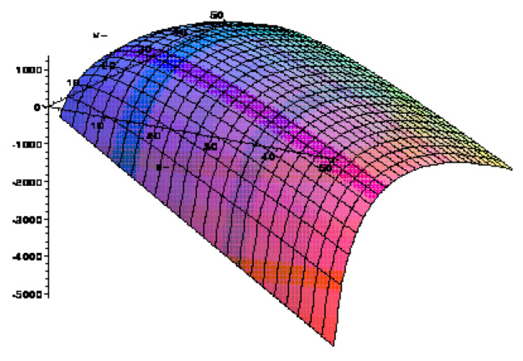
Figure 2 demonstrates simulation results in the reference case. The vertical axis indicates the mean value of accumulated discounted leader’s profit, and two horizontal axes indicate the leader’s instantaneous R&D and manufacturing investment levels respectively. The surface represents the shape of the function

$$\chi (u,v)=\frac{{\int }_0^{\infty }\left[\frac{d_0\sigma v^{\gamma }}{\sigma v^{\gamma }+\left(1-e^{-\beta u_f\frac{{\tau }^2}{2}}\right)Y_f}-(p_{1}u+p_{2}v)\right]e^{-\alpha \tau -\rho u\frac{{\tau }^2}{2}}d\tau }{\alpha {\int }_0^{\infty }{e}^{-\alpha \tau -\rho u\frac{{\tau }^2}{2}}d\tau }.$$

Due to Theorem 1, the maximal value of accumulated discounted leader’s profit corresponds to the maximum value of function $\chi (u,v)$; and values $u_{*}\ge 0$ and $v_{*}>0$, which maximize $\chi (u,v)$, are the leader’s optimal time-invariant R&D and manufacturing investment strategies, respectively.

We perform a sensitivity analysis of the model with respect to the following parameters:

(i)

Market size (demand) $d_0$;

(ii)

R&D price $p_1$;

(iii)

Discount rate $\alpha$;

(iv)

Productivity of the leader $\gamma$;

(v)

R&D efficiency of the leader $\rho$;

(vi)

Level of a typical follower’s investment in R&D $u_f$ (level of competition).

The effects of parameters are easily predictable in some areas and vague in others. One can expect that higher demand will cause higher levels of the leader’s both optimal R&D and manufacturing investment levels, and a higher value of the accumulated discounted profit. Also, one can expect that higher R&D price will cause lower level of the leader’s optimal R&D investments and lower accumulated profit. Higher discount rate means lower present value of future profit. So, it will cause lower optimal R&D investment and lower accumulated profit. It is obvious that higher productivity of the leader yields higher accumulated profit. However, it is vague whether higher productivity causes higher optimal R&D and manufacturing investments. The expectation for the effect of the leader’s productivity is similar to the expectations for the effects of the leader’s R&D efficiency and the level of competition. Higher R&D leader’s efficiency yields higher accumulated profit and higher level of competition yields lower accumulated profit. However, effects of both the leader’s R&D efficiency and the level of competition to the leader’s optimal R&D and manufacturing investments are vague.

(1)

Sensitivity in the market size.

Figure 3 demonstrates the results of sensitivity analysis in the value of market size. Greater market size means relatively strong demand, which yields higher leader’s accumulated profit, and higher optimal R&D and manufacturing investments. It is basically consistent with the expectations. This analysis shows that higher market size stimulates rapid new products development through the higher R&D investments. It suggests that the product life cycle would become shorter and shorter in the industry, where the demand rapidly increases. However, despite that, the demand growth is very fast in the high-tech industry, such as the semiconductor industry, but the product’s life cycle is relatively stable. This difference is due to the fact that the leader’s decision makings are different in the case of the increasing market and in the case of the stable one.

(2)

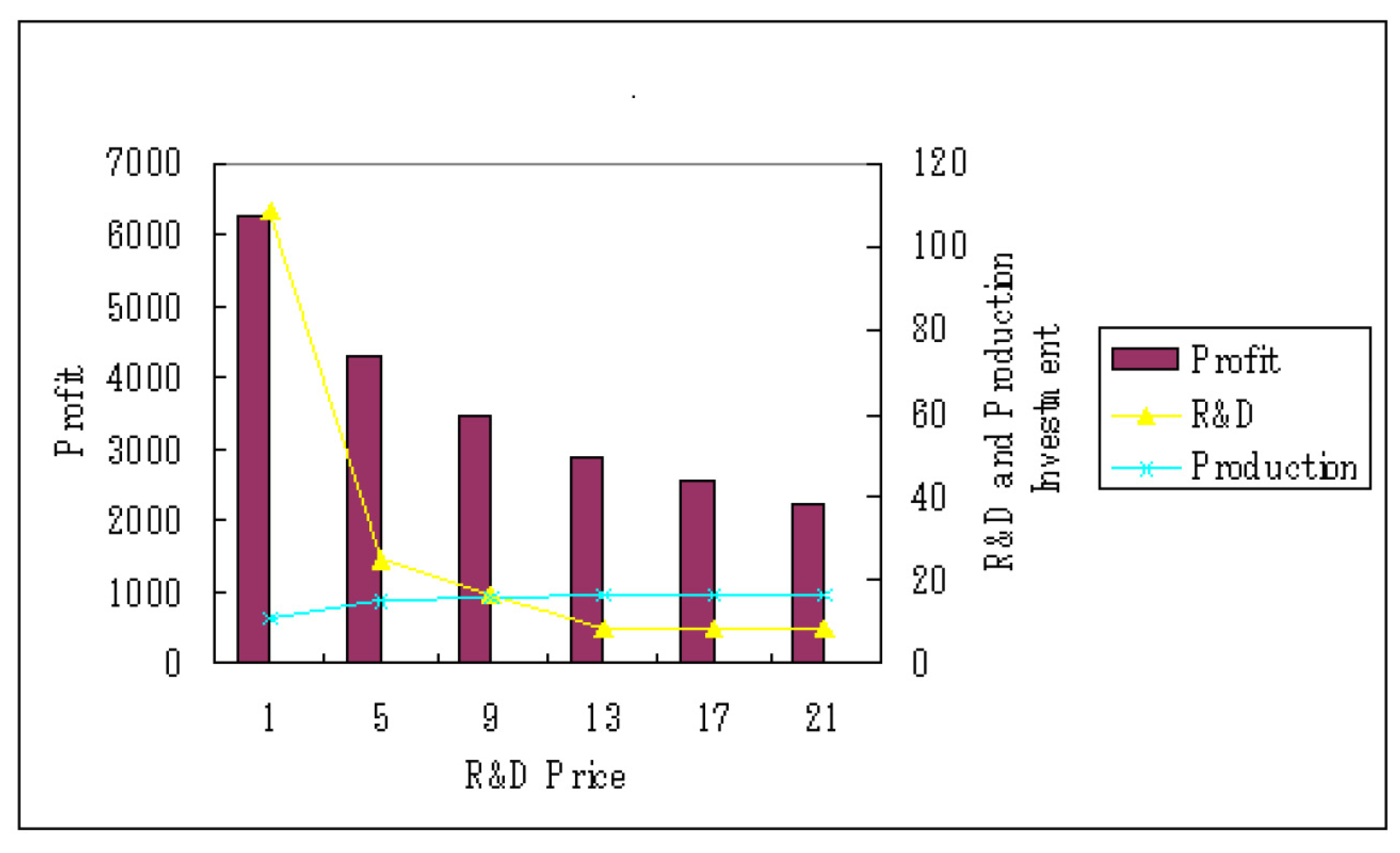
Sensitivity in R&D price.

Figure 4 demonstrates the result of sensitivity analysis in R&D price. Higher R&D price yields lower accumulated profit of the leader and causes lower optimal R&D investments. It is basically consistent with the expectations. Optimal manufacturing investments become larger as R&D price increases. It means that the static social welfare measured by consumer’s surplus increases, while the dynamic social welfare measured by frequency of product generation change as R&D price increases. However, optimal level of manufacturing investments is not so sensitive to the change of R&D price rather than R&D investments. This is because the market size and productivity of the leader are fixed in the model. The relatively large sensitivity of the level of optimal R&D investments in R&D price suggests that the decreasing of R&D cost would be a very effective political instrument for improving social welfare through shortening the product life cycle.

(3)

Sensitivity in discount rate.

Figure 5 demonstrates the result of sensitivity analysis in discount rate. Higher discount rate yields lower accumulated profit, and causes lower optimal R&D investment. Higher discount rate means the future profit gives relatively low utility. It is basically consistent with the expectations. The effect of a discount rate to the optimal manufacturing investment level is relatively small. This is because the manufacturing investment does not heavily depend on the future profit. If the financial market is perfectly competitive, then discount rate is equal to the interest rate. In this case, the rise of the interest rate decelerates the product development through the decreasing of the level of R&D investment.

(4)

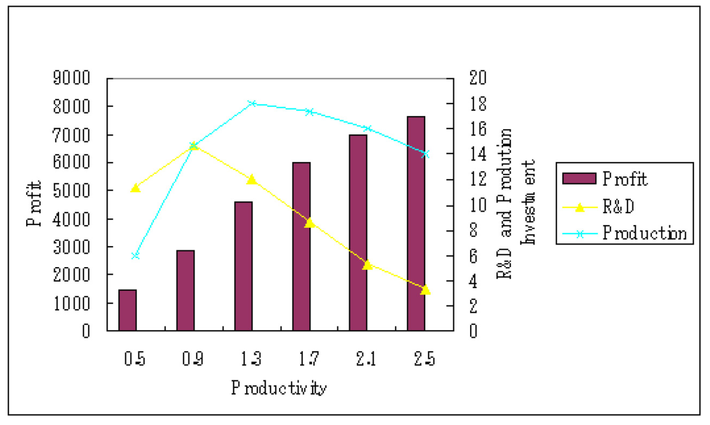
Sensitivity in the leader’s productivity.

Figure 6 demonstrates the result of sensitivity analysis in the leader’s productivity. The result is basically consistent with the expectations. Higher productivity yields higher accumulated profit. Below a certain productivity level (in this case, 0.9 for R&D investments and 1.3 for manufacturing investments), higher productivity causes higher optimal R&D and manufacturing investments. Meanwhile, above the threshold, higher productivity causes lower optimal R&D and production investments. High productivity brings the strong dominant power to the leader. In such a situation, the leader can earn sufficient profit, even in the case of relatively low R&D and manufacturing investments. Thus, higher productivity of the leader provides a negative impact on the new products’ development through the leader’s dominant power. It is interesting that our relatively simple model can handle this monopolistic situation. Note that the leader’s productivity is assumed to be fixed in this model.

This result shows that higher productivity brings the higher static social welfare, while there is an optimal productivity level measured by the dynamic social welfare. If a government intervenes in the productivity of the leader company by imposing regulations or surcharges, it should decide the level of intervention deliberately. The optimal productivity level for the static social welfare measured by consumer’s surplus is different from one for the dynamic social welfare measured by the length of the product life-cycle. The government should consider the balance of these two welfare factors in policy-making.

(5)

Sensitivity in the leader’s R&D efficiency.

Figure 7 demonstrates the result of sensitivity analysis in the leader’s R&D efficiency. It is basically consistent with the expectations. Higher leader’s R&D efficiency yields higher accumulated profit. Above a certain R&D efficiency level, higher R&D efficiency causes lower optimal R&D and manufacturing investments. Meanwhile, below the threshold, higher R&D efficiency causes higher optimal R&D and manufacturing investments.

It is a similar result to the one of sensitivity analysis in the productivity of the leader, but the conclusion for policy implication is different. Higher R&D efficiency brings higher dynamic social welfare, while there is some optimal productivity level measured by the static social welfare. The discussion of this result for policy implications is similar but inverse. If the government intervene R&D efficiency of leader company by imposing regulations or surcharges, it should decide the level of intervention deliberately. The optimal R&D efficiency level for the static social welfare measured by consumer’s surplus is different from one for the dynamic social welfare measured by the length of product life-cycle. The government should consider the balance of these two welfare in its policy-making. However, the effect of the leaders’s productivity to the accumulated profit is larger than the effect of the leader’s R&D efficiency. This is because the leader’s productivity increases its accumulated profit directly through the decreasing of the production cost, while the R&D efficiency increases its profit only through the protection from the penetration of the followers.

(6)

Sensitivity in the level of competition.

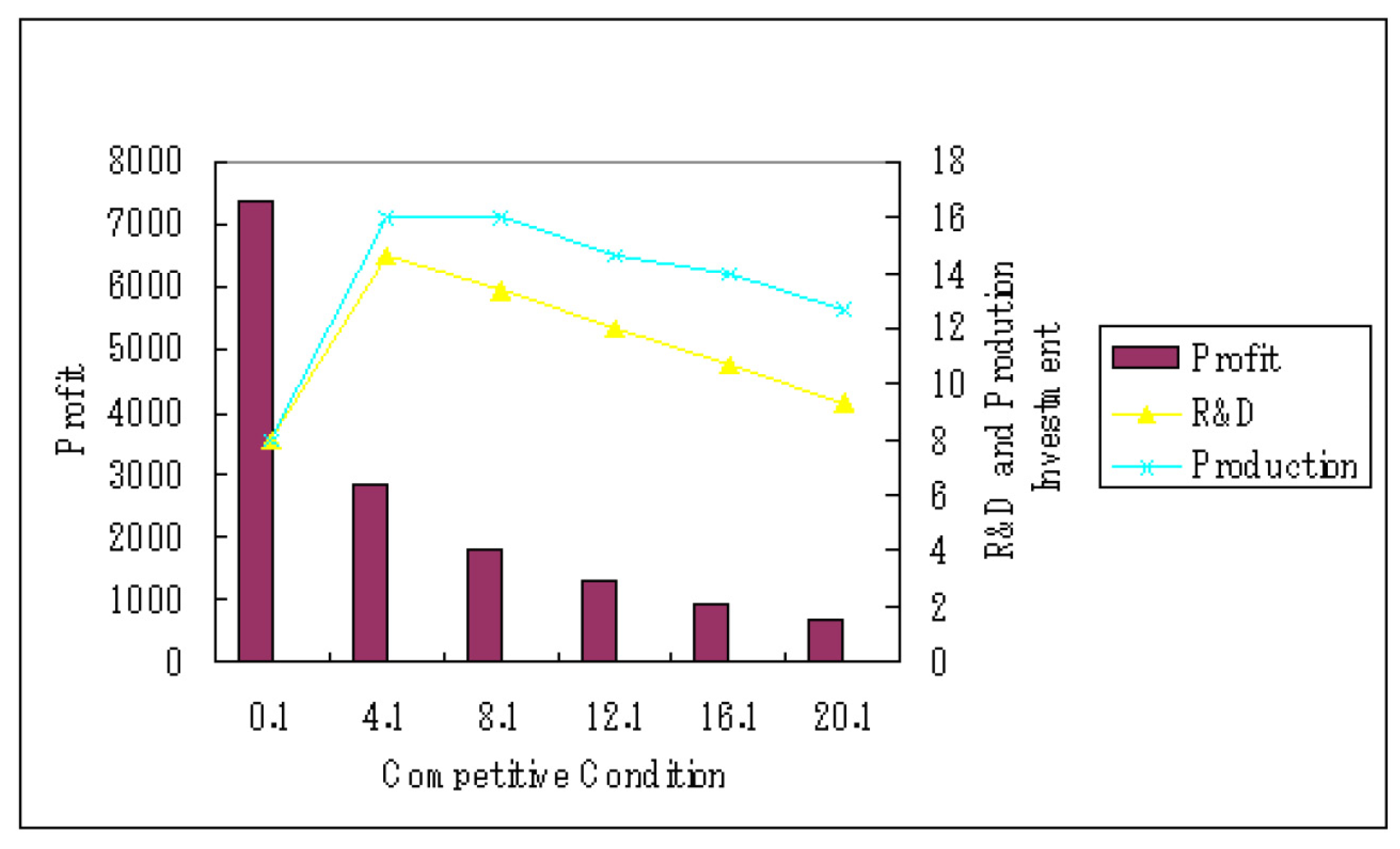
Figure 8 demonstrates the result of sensitivity analysis in the level of competition. It is consistent with the expectation that the harder competition conditions yield less leader’s accumulated profit. For optimal R&D and manufacturing investment policies, we see the concave curves for both optimal levels of R&D and manufacturing investments respectively. Below a certain level of competition (in this case, 4.1), higher competition, which means higher penetration rate of the followers, causes higher optimal R&D and manufacturing investments. While, above the threshold, higher competition causes lower levels of both optimal R&D and manufacturing investments.

This result means that it is very important for the leader to know what kind of investment strategies the followers take. Furthermore, of course, it is also very important for the followers to know what kind of investment strategy the leader takes when they decide on their strategies. This result is also important for policy-making. Concave curves for optimal R&D investment and manufacturing investment mean that these are their optimal competition levels for social welfare. If the government intervene strategy of follower companies by deregulation or subsidization, it should decide the level of intervention deliberately. The optimal competition level for the static social welfare measured by consumer’s surplus is different from the one for the dynamic social welfare measured by the length of the product life-cycle. The government should consider the balance of these two welfare in their policy-making.

6. Concluding Remarks

In this paper, we develop a dynamic model of optimal investment in R&D and manufacturing for a technological leader competing with a large number of identical followers. The model design is based on some general assumptions on probabilistic features of innovation processes. These assumptions lead us to an infinite time horizon stochastic optimization problem. Nevertheless, our main result (Theorem 1) is completely deterministic. It provides a tool for analytic studies and numerical simulations.

In the case when the technological leader competes with a large number of identical followers, the following effects of the model parameters are obtained due to the numerical simulations:

(i)

Higher demand yields higher accumulated profit of the leader and higher optimal R&D and manufacturing investments;

(ii)

Higher R&D price yields lower accumulated profit of the leader and lower optimal R&D investments. It causes relatively stable optimal manufacturing investments;

(iii)

Higher discount rate yields lower accumulated profit and causes lower optimal R&D investments level. It has little effect on the manufacturing investments level;

(iv)

Higher productivity of the leader yields higher accumulated profit. Below a certain productivity level, higher productivity causes higher optimal R&D and manufacturing investments. Meanwhile, above the threshold, higher productivity causes lower optimal R&D and manufacturing investments;

(v)

Higher R&D efficiency of the leader yields higher accumulated profit. Above a certain R&D efficiency level, higher R&D efficiency causes lower optimal R&D and manufacturing investments. Meanwhile, below the threshold, higher R&D efficiency causes higher optimal R&D and manufacturing investments;

(vi)

Higher level of competition yields smaller leader’s accumulated profit. Below a certain competition level, higher competition, which means higher penetration rate of the followers, causes higher optimal R&D and manufacturing investments. Meanwhile, above the threshold, higher competition causes lower optimal R&D and manufacturing investments.

These results suggest interesting policy implications from the point of view of static and dynamic social welfare. Manufacturing investment relates to the static social welfare measured by consumer’s surplus. R&D investment relates to the dynamic social welfare measured by the length of the production life-cycle. Our sensitivity analysis demonstrates concave curves of optimal manufacturing investments and (or) R&D investments. These results suggest that there are optimal levels of policy intervention for static and dynamic social welfare, respectively. The government policy maker should decide the level of policy intervention deliberately and consider the balance between the static and dynamic social welfare. For example, policy intervention to the dominant company, such as Microsoft and Intel, observed commonly in high-tech industries, should be executed after deep consideration about both static and dynamic social welfare.

To conclude, we note that behaviors of innovators acting on the market of a technological product can be studied from different points of view. In the present paper, we are focused on the consideration of the innovation race from the point of view of the technological leader. However, we believe that the developed methodology could be useful for studying of similar models which consider the situation from the opposite point of view of followers, or even in the case when a follower can overtake the leader.

References

- Kuhn, T. The Structure of Scientific Revolutions; University of Chicago Press: Chicago, IL, USA, 1970. [Google Scholar]
- Dosi, G. Technological paradigms and technological trajectories. Res. Policy 1982, 11, 147–162. [Google Scholar] [CrossRef]
- Victor, N.M. DRAMs as model organisms for study of technological evolution. Technol. Forecast. Social Chang. 2002, 69, 243–262. [Google Scholar] [CrossRef]
- Mukoyama, T. Innovation, imitation, and growth with cumulative technology. J. Monet. Econ. 2003, 50, 361–380. [Google Scholar] [CrossRef]
- Porter, M. Competitive Advantage: Creating and Sustaining Superior Performance; Free Press: New York, NY, USA, 1985. [Google Scholar]
- Levin, R.C.; Klevorick, A.K.; Nelson, R.R.; Winter, S.G. Appropriating the returns form industrial research and development. Brook. Pap. Econ. Act. 1987, 3, 839–916. [Google Scholar]
- Teece, D.J. Profiting from technological innovation: implications for integration, collaboration, licensing and public policy. Res. Policy 1986, 15, 285–306. [Google Scholar] [CrossRef]
- Goto, A.; Nagata, A. Appropiability of Innovation and Technological Opportunity; National Institute for Science and Technology Policy: Tokyo, Japan, 1997.
- Mansfield, E.; Schwartz, M.; Wagner, S. Imitation costs and patents: an empirical study. Econ. J. 1981, 91, 907–918. [Google Scholar] [CrossRef]
- Lieberman, M.B.; Montgomery, D.B. First-mover advantages. Strateg. Manag. J. 1988, 9, 41–58. [Google Scholar] [CrossRef]
- Ishida, M.; Matsumara, T.; Matsushima, N. Market competition, R&D and firm profits in asymmetric oligopoly. J. Ind. Econ. 2011, 59, 484–505. [Google Scholar]
- Ofek, E.; Sarvary, M. R&D, marketing, and the success of next-generation products. Mark. Sci. 2003, 22, 355–370. [Google Scholar]
- Parra, Á. Sequential innovation, patent policy, and the dynamics of the replacement effect. RAND J. Econ. 2019, 50, 568–590. [Google Scholar] [CrossRef] [Green Version]
- Cohen, M.A.; Eliashberg, J.; Ho, T.-H. New product development: The performance and time-to-market trade off. Manag. Sci. 1996, 42, 173–186. [Google Scholar] [CrossRef] [Green Version]
- Bayus, B.L. Speed-to-market and new product performance trade-offs. J. Prod. Manag. 1997, 14, 485–497. [Google Scholar] [CrossRef]
- Morgan, L.O.; Morgan, R.M.; Moore, W.L. Quality and time-to-market trade-offs when there are multiple product generations. Manuf. Serv. Oper. Manag. 2001, 3, 89–104. [Google Scholar] [CrossRef]
- Cohen, M.A.; Eliashberg, J.; Ho, T.-H. An anatomy of a decision-support system for developing and launching line extensions. J. Mark. Res. 1997, 34, 117–129. [Google Scholar] [CrossRef] [Green Version]
- Ramdas, K.; Swahney, M.S. A cross-functional approach to evaluating multiple line extensions for assembled products. Manag. Sci. 2001, 47, 22–36. [Google Scholar] [CrossRef]
- Paulson Gjerde, K.A.; Slotnick, S.A.; Sobel, M.J. New product innovation with multiple features and technology constraints. Manag. Sci. 2002, 48, 1268–1284. [Google Scholar] [CrossRef] [Green Version]
- Souza, G.C.; Bayus, B.L.; Wagner, H.M. New-product strategy and industry clockspeed. Manag. Sci. 2004, 50, 537–549. [Google Scholar] [CrossRef]
- Reinganum, J.F. On the diffusion of new technology: A game theoretic approach. Rev. Econ. Stud. 1981, 48, 395–405. [Google Scholar] [CrossRef]
- Breitmoser, Y.; Tan, J.H.W.; Zizzo, D.J. Understanding perpetual R&D races. Econ. Theory 2010, 44, 445–567. [Google Scholar]
- Aghion, P.; Howitt, P. A model of growth through creative destruction. Econometrica 1992, 60, 323–351. [Google Scholar] [CrossRef]
- Aghion, P.; Bechtold, S.; Cassar, L.; Herz, H. The causal effects of competition on innovation: experimental evidence. J. Law Econ. Organ. 2018, 34, 162–195. [Google Scholar] [CrossRef] [Green Version]
- Meissner, D.; Kotsemir, M. Conceptualizing the innovation process towards the “active innovation paradigm”—Trends and outlook. J. Innov. Entrep. 2016, 5, 1–18. [Google Scholar] [CrossRef] [Green Version]
- Morone, P.; Taylor, R. Knowledge Diffusion and Innovation. Modelling Complex Entrepreneurial Behaviours; Edward ElgarPublishing Ltd.: Cheltenham, UK; Northampton, MA, USA, 2010. [Google Scholar]
- Arrow, K.J.; Kurz, M. Public Investment, the Rate of Return and Optimal Fiscal Policy; Jons Hopkins University Press: Baltimore, MD, USA, 1970. [Google Scholar]
- Baro, R.; Sala-i-Martin, X. Economic Growth; McGraw Hill: New York, NY, USA, 1995. [Google Scholar]
- Grossman, G.M.; Helpman, E. Innovation and Growth in the Global Economy; The MIT Press: Cambridge, MA, USA, 1991. [Google Scholar]
- Carlson, D.A.; Haurie, A.B.; Leizarowitz, A. Infinite Horizon Optimal Control: Determenistic and Stochastic Systems; Springer: Berlin, Germany, 1991. [Google Scholar]
- Galbraith, J.R. Designing the Innovating Organization; G 99-7 (366); CEO Publication: Los Angeles, CA, USA, 1999. [Google Scholar]
- Gnedenko, B.V. The Theory of Probability; Chelsea Publishing Company: New York, NY, USA, 1962. [Google Scholar]
- Intriligator, M. Mathematical Optimization and Economic Theory; Prentice-Hall: New York, NY, USA, 1971. [Google Scholar]
- Winter, S.G.; Kaniovski, Y.M.; Dosi, G. Modeling industrial dynamics with innovative entrants. Struct. Econ. Dyn. 2000, 11, 255–293. [Google Scholar] [CrossRef] [Green Version]