A Stochastic Characterization of the Capture Zone in Pursuit-Evasion Games


Department of Engineering and Mathematics, Sheffield Hallam University, Howard Street, Sheffield S1 1WB, UK
Games 2020, 11(4), 54; https://0-doi-org.brum.beds.ac.uk/10.3390/g11040054
Submission received: 10 October 2020
/
Revised: 8 November 2020
/
Accepted: 16 November 2020
/
Published: 20 November 2020
(This article belongs to the Special Issue Optimal Control Theory)
Abstract
:Pursuit-evasion games are used to define guidance strategies for multi-agent planning problems. Although optimal strategies exist for deterministic scenarios, in the case when information about the opponent players is imperfect, it is important to evaluate the effect of uncertainties on the estimated variables. This paper proposes a method to characterize the game space of a pursuit-evasion game under a stochastic perspective. The Mahalanobis distance is used as a metric to determine the levels of confidence in the estimation of the Zero Effort Miss across the capture zone. This information can be used to gain an insight into the guidance strategy. A simulation is carried out to provide numerical results.
1. Introduction
Pursuit-evasion differential games have been applied to autonomous vehicles guidance problems in various contexts ranging from missile guidance [1], to spacecraft orbital maneuvers [2], and mobile robots [3]. Since their introduction in [4], other versions have been formulated, including stochastic [5] and multi-agent [6] games.
A common solution for simplifying the architectures and reducing the weights and costs of autonomous vehicles is to adopt a single instrument (bearing or range sensor) for target tracking or navigation [7,8]. This work focuses on a missile application, but the results can be easily extended to other scenarios and to different sets of measurements. In missile systems, passive sensors like electro-optical or optical seekers are often used to provide the target direction with respect to the vehicle. This bearings-only measurement system comes at the cost of not having information on the range to the target when an optimal guidance law is employed. To enhance the observability of the range and, therefore, to improve the performance of the engagement, it is necessary to deviate from the optimal guidance strategy. Different strategies for optimizing these maneuvers have been extensively studied in the literature. Reference [9] looks at the maneuver that maximizes the determinant of the Fisher information matrix, while [10] maximizes the eigenvalues of the normalized error covariance matrix; reference [11] tries to maintain the line of sight rate larger than a certain threshold, while [12] imposes different intercept angles between consecutive pursuers, and [13] uses a performance measure of observability based on geometric conditions.
Two stochastic metrics that have found application in the study of maneuvers effects on target estimation with different sets of sensors are the Cramér–Rao lower bound (CRLB) [14,15] and the Fisher information [16,17]. The CRLB returns an indication of the performance of a maximum likelihood estimator in terms of error covariance. The Fisher information is related to the CRLB by an inverse relationship, as will be shown later in the paper. An issue related to the use of these metrics in missile applications is that, for an unobservable system, their numerical computation can be prone to errors because the Fisher information matrix would result in being nonsingular [18].
Rather than a new sub-optimal guidance law to optimize maneuvers, this paper proposes a method for characterizing the game space of a pursuit-evasion game using another stochastic metric, the Mahalanobis distance, which can be calculated independently from the CRLB and the Fisher information and thus will suffer less from numerical issues. The proposed method allows for obtaining a map of the confidence in the estimation of the main variable of a pursuit-evasion guidance law, called the Zero Effort Miss (ZEM). This knowledge can be exploited as a cost to numerically minimize in guidance algorithms or as an information to feed reinforcement learning algorithms [19]. An advantage of this solution is that it is not computationally heavy, as it only involves the calculation of the Mahalanobis distance from the covariance matrix of the Kalman filter.
2. Statement of the Problem
2.1. Engagement Description
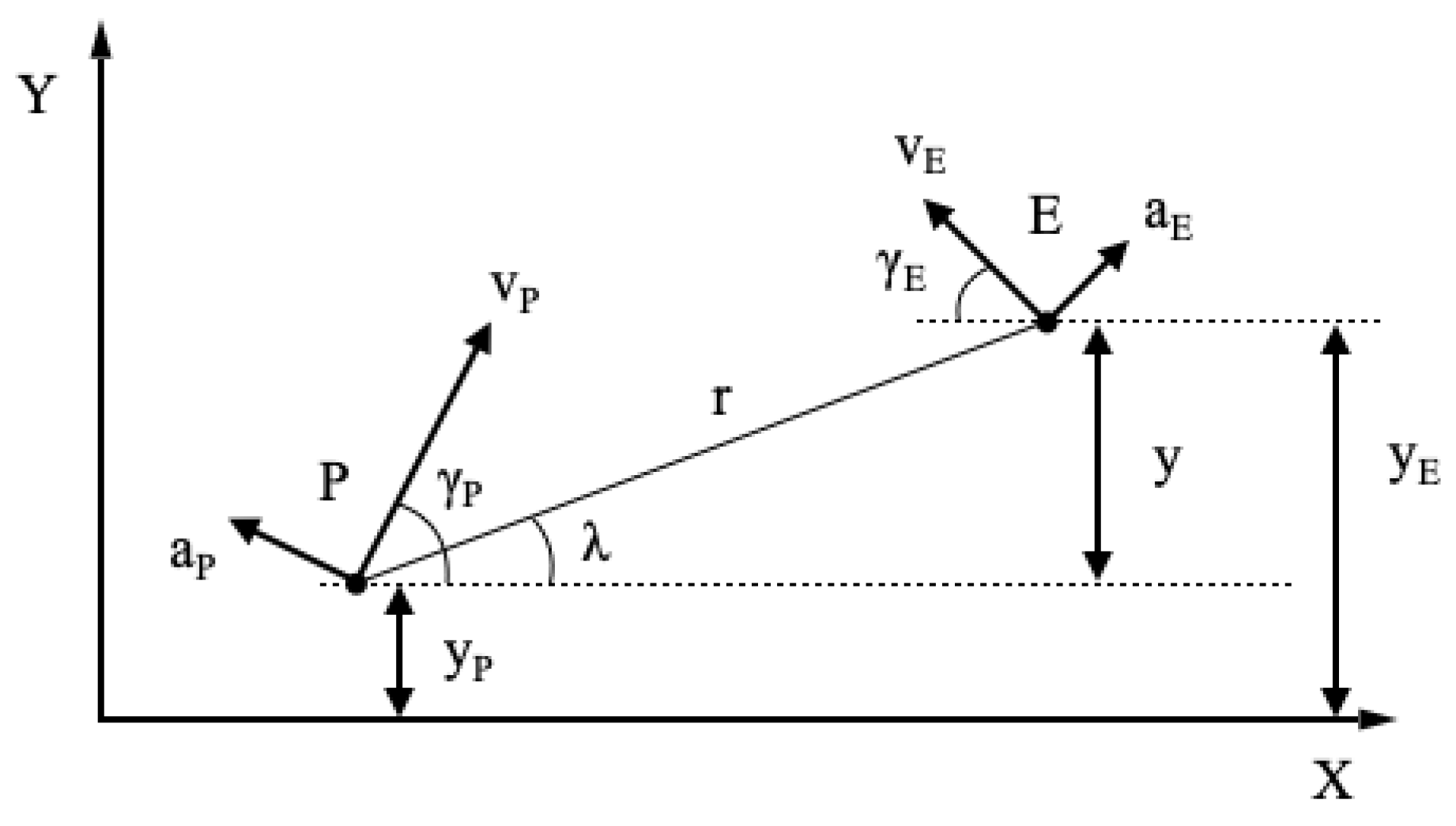
Consider the pursuer P and the evader E represented in Figure 1 in a Cartesian reference frame of coordinates . P and E are assumed to be mass points, with constant speeds and , and lateral accelerations and , respectively. The distance between P and E is the relative range r. The line of sight (LOS) forms an angle with the horizontal reference. The flight path angles of the pursuer and the evader are indicated as and , respectively. The vertical coordinates of the two players are and
The dynamics of the engagement assumes that the physical systems implementing the guidance commands u and v can be represented as first order systems with time constants and , respectively. The set of nonlinear equations that describes the dynamics of the engagement is resumed in Equation (1):
Under the assumption of small LOS angle , the miss y can be approximated as
Assuming also that and are small, the nonlinear model of Equation (1) can be linearized obtaining a new system [20]:
whose state vector X is defined as:
and the matrices are:
The control inputs u and v are normalized with the maximum lateral acceleration values and , respectively, resulting in a system with bounded controls ().
2.2. Pursuit-Evasion Games
A differential game can be set up to obtain optimal guidance strategies and for the linear system with bounded controls of Equation (3). This kind of differential game is called a pursuit-evasion game because the optimal strategies aim at minimizing (the pursuer) or maximizing (the evader) the relative distance at the final time , called miss distance. One of the most important features of the pursuit-evasion games formulation is the definition of a structure for the game space with capture and avoidance regions where finite miss is guaranteed. Depending on the characteristics of the two players (time constants and maximum accelerations), a number of structures can be defined [20] with semipermeable bounds that can be calculated integrating backwards the derivative from its final condition :
where and are the values of the relative angles around which the linearization has been performed.
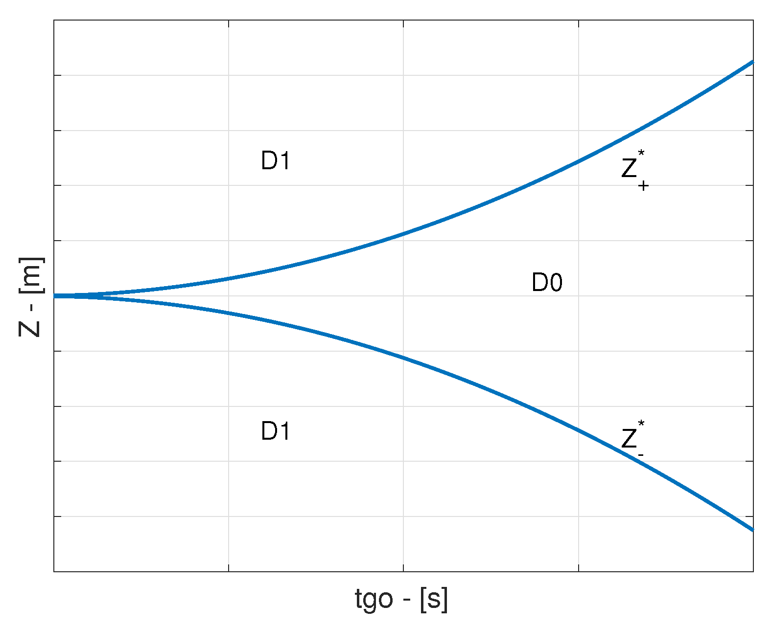
Figure 2 shows a game structure with the bounds plotted against the time-to-go to the interception for the case where and . The capture zone , in this case, is a region where optimal strategies are arbitrary and zero miss is guaranteed. The avoidance zone is a region where zero miss can not be achieved and the optimal commands are
The ZEM in the previous equation is the final distance between the two players at the end of the engagement assuming no further maneuvers from the players. The expression for the engagement of Equation (1) is given by:
with being approximated as:
If the pursuer starts the engagement in the capture zone and, if it adopts the guidance strategy of Equation (9), the level of will remain close to 0. A different guidance command will produce a larger , approaching the bounds .
2.3. Estimator in the Loop
The implementation of the guidance strategy of Equation (9) requires the knowledge of an estimate of the , which is made up of information on both the pursuer and the evader states. Pursuer’s related variables such as , , and can be provided by the on-board navigation system, but the other variables need to be reconstructed through an estimator, in most cases a nonlinear Kalman filter. The vector of variables that need to be estimated is therefore:
In the case of a seeker measuring the LOS angle (bearings-only measurements, BOM):
If a relative range measurement is available too, Equation (13) is updated as:
The noise signals and , are defined as zero-mean Gaussian sequences with variance and , respectively. The model provided to the Kalman Filter includes a shaping filter to represent target maneuvers, which are assumed as maximum acceleration maneuvers whose starting time is uniformly distributed over the flight time. The maneuvers model provided to the filter is a white noise with spectral density through an integrator [21]. The complete model is given by:
The Jacobian matrix J associated with the previous model can be found in [10] and it is used along with the sample time to calculate the state transition matrix :
It is well known that, in the case of bearings-only measurements, becomes unobservable if the pursuer is maintained on the collision triangle, i.e., if an optimal guidance law such as that of Equation (9) is applied. To gain an insight on range observability, one should maneuver away from the collision triangle, at the cost of increasing the . This does not preclude capture until the D0 region is not abandoned, but since the is only available as an estimation, there is the risk of getting too close to the borders of D0 or even to pass in the D1 zone.
3. Characterization of the Game Structure
It is very important for the pursuer to have a good estimate of the so as to apply the best guidance command possible. In addition, if the adopted guidance strategy does not intend to maintain the around 0, it is crucial to know how good its estimate is. Although can be calculated exactly using a regressive value, its distance from the estimated is random, since is itself a random variable. It seems interesting, therefore, to characterize the D0 region in terms of a stochastic metric. To this purpose, the concept of Mahalanobis distance will be introduced in this section, along with the CRLB of the estimator considered in this study.
3.1. Mahalanobis Distance
The Mahalanobis distance between a random variable and a point is defined as:
where is the covariance matrix associated with the random variable . represents a region in the neighborhood of where should be. In other words, is a measurement of the confidence in the estimation of the real parameter : a null means that coincides with the mean of ; a larger means that the estimation of is less correct. The interest of this work lies in determining the confidence on the estimation of the at each value of . To this end, a Mahalanobis distance for is defined as:
The covariance can be obtained at each time instant using the value of the error covariance of the Kalman filter. This can be easily done on the go, i.e., in real time with the estimator, returning a value of that depends on the features of the filtering algorithm (e.g., approximation of the nonlinear dynamics, tuning parameters, etc.). As a mean of comparison, another covariance can be used in the calculation, which is that obtained through the CRLB associated with the estimator. This can be interpreted as an ideal performance test, as it would return the minimum value for , independent from the filtering algorithm.
3.2. Cramér–Rao Bound
The CRLB is defined as the minimum estimation covariance bound of an unbiased estimator. In practice, it tells how good an estimator can theoretically be, given a noisy measurement. An estimator is called efficient if its variance is equal to the CRLB, meaning that its mean squared estimation error is the lowest possible among all unbiased estimators. Such an estimator is sometimes called not practical, as it would yield the best theorical performance. According to the Cramér–Rao theorem, the minimum variance of an unbiased estimator of the parameter is always larger than the inverse of the associated Fisher information matrix F [22]:
where f is the likelihood function of the n measurements sequence z given .
The CRLB of a function of the parameter is given by:
In this work, the function g is the of Equation (10), while is the vector of Equation (12). When the estimation is carried out using a Kalman filter, as in this work, the Fisher information matrix of Equation (20) at the k-th step can be written in a recursive form [23]:
The initial condition on F is defined considering a filter with infinite initial error covariance matrix, therefore:
4. Numerical Example
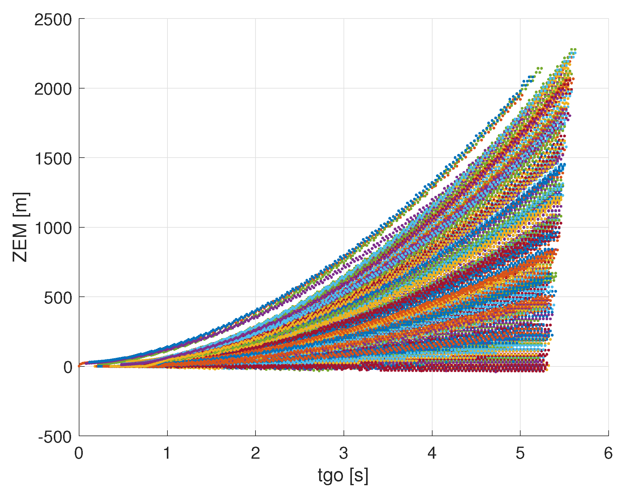
Two numerical simulations, each one consisting of 200 Monte Carlo runs, were carried out to calculate the values of across the D0 region. The first simulation uses both bearings and range measurements as in Equation (14), while the second employs the bearings-only measurements of Equation (13). Different paths are travelled in each run of the simulation in order to cover the entire D0 region, as shown in Figure 3, where each colour represents a different run. The trajectories of both players for a single run are shown in Figure 4. The Mahalanobis distance is calculated in correspondence of each dot of Figure 3 in two ways: first using the values of the CRLB from Equation (22) as the covariance in Equation (18), and then using the error covariance matrix calculated by the filter. The numerical initial values (, , , , , ) and parameters used in the simulations are reported in Table 1.
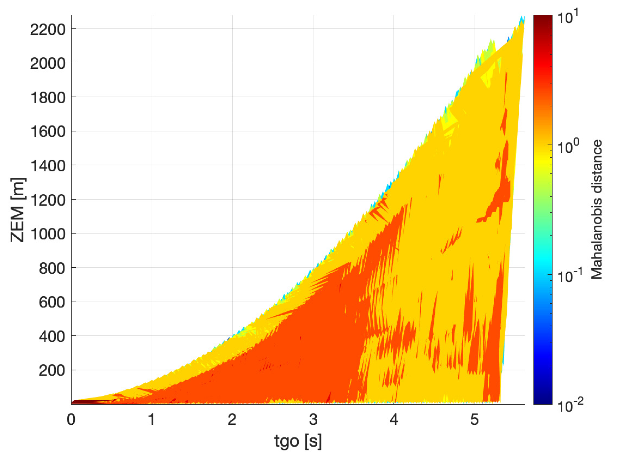
Figure 5 and Figure 6 show the result of the simulation for the case of bearings and range measurements. The levels of the Mahalanobis distance are associated with different colors in the maps, as indicated in the sidebar. The red regions are those where the estimation of is worse, and the blue regions where it is best. The maps are generated by merging the results of all the runs at each time instant. The value of the Mahalanobis distance in Figure 5 is calculated using the CRLB, while that in Figure 6 is obtained from the filter. At the beginning of the engagement ( s), the value of in Figure 5 is very low and increases as the engagement moves on. This is a consequence of the initialization of the Fisher information in this method (Equation (24)). Since the CRLB is the inverse of the Fisher information, the initial will be very large and, therefore, will be very small at the beginning. Since in the case of Figure 6 the initial covariance is finite, the value of at the beginning is larger than in Figure 5, which is more realistic, as the uncertainty over the estimation of a variable is finite in practice. Another difference is that the levels of Mahalanobis distance obtained with the CRLB are lower than those calculated through the filter. However, this was expected as the CRLB is an ideal bound for the estimator and the performance of a practical filter is always worse. A feature in common for the two cases is that is smaller in the proximity of the upper bound . This can be explained with the observability improvement obtained when maneuvering away from the collision triangle, even though the range measurements here already provide a certain level of observability. The high levels of towards the end of the engagement suggest that then it is risky to maneuver away from the collision triangle because a last-minute maneuver from the evader might suddenly increase the and cause the passage to the avoidance zone.
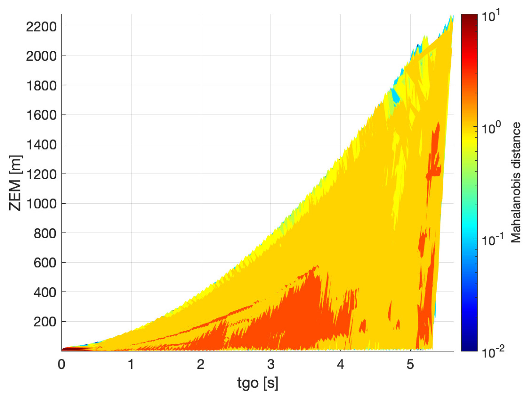
The case of bearings-only measurements is presented in Figure 7 and Figure 8. The results obtained with the CRLB are prone to numerical issues due to the fact that the system in this case is unobservable, and therefore a good portion of the data at the beginning of the engagement is missing in Figure 7. The matrix computed through Equation (23) is not invertible and therefore the CRLB cannot be initially calculated. The values of obtained from the filter (Figure 8) in the first instants of the engagement ( > 4 s) are similar to those of Figure 6: this is no surprise as the filter is initialized in the same way in both cases. As the engagement moves on, the tendency of having smaller values of (and hence a better estimation of the ) in the proximity of the bound is even more evident than in the previous case: the 0 level of the is characterized by a red strip, while yellow and even blue layers can be found next to the bound. Since there are no range measurements here, the only way to enhance the observability is to maneuver away from the collision triangle, evidently. As in the case of bearings and range measurements, the values of are larger when calculated through the filter (Figure 8) than when computed through the CRLB (Figure 7).
5. Conclusions
Pursuit-evasion games offer a compact solution to the problem of target interception or rendez-vous for autonomous vehicles, but need to rely on a good estimation of the variables needed in the guidance formulation. This is not always possible, as the number of on-board sensors is often limited by weights and cost constraints.
This paper has presented a method for characterizing the capture region of a pursuit-evasion game in terms of the confidence on the estimation of the . The method consists of calculating the Mahalanobis distance associated with the estimated by the on-board nonlinear filter. A comparison with the Mahalanobis distance obtained through the CRLB showed that the proposed method provides consistent results, which are less prone to numerical issues than the other.
These results can be used to design modern guidance laws that consider observability issues in their formulation, in addition to the classic considerations on miss distance and control effort minimization. This is especially valuable in scenarios where not all the necessary sensors are available, but there is a demand for high performance in terms of accuracy.
Funding
This research received no external funding.
Acknowledgments
The author would like to thank Henrique T.M. Menegaz (University of Brasília, Brazil) for the discussions on the use of the Mahalanobis distance in estimation problems.
Conflicts of Interest
The author declares no conflict of interest.
References
- Shinar, J. Solution techniques for realistic pursuit-evasion games. In Control and Dynamic Systems; Elsevier: New York, NY, USA, 1981; Volume 17, pp. 63–124. [Google Scholar]
- Pontani, M.; Conway, B.A. Numerical solution of the three-dimensional orbital pursuit-evasion game. J. Guid. Control Dyn. 2009, 32, 474–487. [Google Scholar] [CrossRef]
- Chung, T.H.; Hollinger, G.A.; Isler, V. Search and pursuit-evasion in mobile robotics. Auton. Robot. 2011, 31, 299. [Google Scholar] [CrossRef] [Green Version]
- Isaacs, R.P. Differential Games; John Wiley and Sons: Hoboken, NJ, USA, 1965. [Google Scholar]
- Yavin, Y.; De Villiers, R. Stochastic pursuit-evasion differential games in 3D. J. Optim. Theory Appl. 1988, 56, 345–357. [Google Scholar] [CrossRef]
- Hayoun, S.Y.; Shima, T. A Two-on-One Linear Pursuit–Evasion Game with Bounded Controls. J. Optim. Theory Appl. 2017, 174, 837–857. [Google Scholar] [CrossRef]
- Stegagno, P.; Cognetti, M.; Oriolo, G.; Bülthoff, H.H.; Franchi, A. Ground and aerial mutual localization using anonymous relative-bearing measurements. IEEE Trans. Robot. 2016, 32, 1133–1151. [Google Scholar] [CrossRef] [Green Version]
- He, S.; Shin, H.S.; Tsourdos, A. Optimal active target localisation strategy with range-only measurements. In Proceedings of the 16th International Conference on Informatics in Control, Automation and Robotics, Prague, Czech Republic, 29–31 July 2019. [Google Scholar]
- Oshman, Y.; Davidson, P. Optimization of observer trajectories for bearings-only target localization. IEEE Trans. Aerosp. Electron. Syst. 1999, 35, 892–902. [Google Scholar] [CrossRef]
- Battistini, S.; Shima, T. Differential games missile guidance with bearings-only measurements. IEEE Trans. Aerosp. Electron. Syst. 2014, 50, 2906–2915. [Google Scholar] [CrossRef]
- Seo, M.G.; Tahk, M.J. Observability analysis and enhancement of radome aberration estimation with line-of-sight angle-only measurement. IEEE Trans. Aerosp. Electron. Syst. 2015, 51, 3321–3331. [Google Scholar]
- Fonod, R.; Shima, T. Estimation enhancement by cooperatively imposing relative intercept angles. J. Guid. Control Dyn. 2017, 40, 1711–1725. [Google Scholar] [CrossRef]
- He, S.; Shin, H.S.; Tsourdos, A. Trajectory optimization for target localization with bearing-only measurement. IEEE Trans. Robot. 2019, 35, 653–668. [Google Scholar] [CrossRef] [Green Version]
- Fawcett, J.A. Effect of course maneuvers on bearings-only range estimation. IEEE Trans. Acoust. Speech Signal Process. 1988, 36, 1193–1199. [Google Scholar] [CrossRef]
- Roh, H.; Shim, S.W.; Tahk, M.J. Maneuver Algorithm for Bearings-Only Target Tracking with Acceleration and Field of View Constraints. Int. J. Aeronaut. Space Sci. 2018, 19, 423–432. [Google Scholar] [CrossRef]
- Wang, X.; Cheng, Y.; Moran, B. Bearings-only tracking analysis via information geometry. In Proceedings of the 2010 13th International Conference on Information Fusion, Edinburgh, UK, 26–29 July 2010; pp. 1–6. [Google Scholar]
- Cheng, Y.; Wang, X.; Morelande, M.; Moran, B. Information geometry of target tracking sensor networks. Inf. Fusion 2013, 14, 311–326. [Google Scholar] [CrossRef]
- Jauffret, C. Observability and Fisher information matrix in nonlinear regression. IEEE Trans. Aerosp. Electron. Syst. 2007, 43, 756–759. [Google Scholar] [CrossRef]
- Gaudet, B.; Furfaro, R.; Linares, R. Reinforcement learning for angle-only intercept guidance of maneuvering targets. Aerosp. Sci. Technol. 2020, 99, 105746. [Google Scholar] [CrossRef] [Green Version]
- Shima, T.; Shinar, J. Time-varying linear pursuit-evasion game models with bounded controls. J. Guid. Control Dyn. 2002, 25, 425–432. [Google Scholar] [CrossRef]
- Zarchan, P. Representation of realistic evasive maneuvers by the use of shaping filters. J. Guid. Control 1979, 2, 290–295. [Google Scholar] [CrossRef]
- Kay, S.M. Fundamentals of Statistical Signal Processing; Prentice Hall PTR: Upper Saddle River, NJ, USA, 1993. [Google Scholar]
- Taylor, J. The Cramer-Rao estimation error lower bound computation for deterministic nonlinear systems. IEEE Trans. Autom. Control 1979, 24, 343–344. [Google Scholar] [CrossRef]
Figure 1.
Engagement scenario.

Figure 2.
A pursuit-evasion game structure.

Figure 3.
True ZEM for the simulated cases.

Figure 4.
Trajectory of both players in the coordinates for one of the runs.

Figure 5.
calculated with CRLB—Bearings + Range measurements.

Figure 6.
from the filter—Bearings + Range measurements.

Figure 7.
calculated with CRLB—Bearings only measurement.

Figure 8.
from the filter—Bearings only measurement.


Table 1.
Simulation initial values and parameters.
| Parameter | Value | Parameter | Value |
|---|---|---|---|
| 3 km/s | 1.2 km/s | ||
| 30 g | 10 g | ||
| 10 km | |||
| (, ) | g | 9.81 m/s | |
| 0 m/s | 0 m/s | ||
| 0.1 s | 0.2 s | ||
| 0.02 s | |||
| 0.001 rad | 50 m |
Publisher’s Note: MDPI stays neutral with regard to jurisdictional claims in published maps and institutional affiliations. |
© 2020 by the author. Licensee MDPI, Basel, Switzerland. This article is an open access article distributed under the terms and conditions of the Creative Commons Attribution (CC BY) license (http://creativecommons.org/licenses/by/4.0/).
Share and Cite
MDPI and ACS Style
Battistini, S. A Stochastic Characterization of the Capture Zone in Pursuit-Evasion Games. Games 2020, 11, 54. https://0-doi-org.brum.beds.ac.uk/10.3390/g11040054
AMA Style
Battistini S. A Stochastic Characterization of the Capture Zone in Pursuit-Evasion Games. Games. 2020; 11(4):54. https://0-doi-org.brum.beds.ac.uk/10.3390/g11040054
Chicago/Turabian StyleBattistini, Simone. 2020. "A Stochastic Characterization of the Capture Zone in Pursuit-Evasion Games" Games 11, no. 4: 54. https://0-doi-org.brum.beds.ac.uk/10.3390/g11040054
Note that from the first issue of 2016, this journal uses article numbers instead of page numbers. See further details here.