A Survey on Nonstrategic Models of Opinion Dynamics

1
Centre d’Economie de la Sorbonne, 106-112 Bd de l’Hôpital, 75647 Paris, France
2
Paris School of Economics, Université Paris 1 Panthéon-Sorbonne, 75231 Paris, France
3
Paris School of Economics, CNRS, 75016 Paris, France
*
Author to whom correspondence should be addressed.
Games 2020, 11(4), 65; https://0-doi-org.brum.beds.ac.uk/10.3390/g11040065
Submission received: 28 October 2020
/
Revised: 4 December 2020
/
Accepted: 10 December 2020
/
Published: 17 December 2020
(This article belongs to the Special Issue Social and Economic Networks)
Abstract
:The paper presents a survey on selected models of opinion dynamics. Both discrete (more precisely, binary) opinion models as well as continuous opinion models are discussed. We focus on frameworks that assume non-Bayesian updating of opinions. In the survey, a special attention is paid to modeling nonconformity (in particular, anticonformity) behavior. For the case of opinions represented by a binary variable, we recall the threshold model, the voter and q-voter models, the majority rule model, and the aggregation framework. For the case of continuous opinions, we present the DeGroot model and some of its variations, time-varying models, and bounded confidence models.
1. Introduction
Although for some issues and specific topics, opinions can be formed immediately and do not change over time despite possible interactions between individuals, in most real-life situations, opinion formation is a rich, complex, and dynamic process. For example, in any society individuals’ views on numerous economic, societal, and political issues are usually formed via a process of opinion dynamics, caused by interactions among the individuals. The central question is: How can the opinion of a society evolve, due to various influence phenomena?
Opinion dynamics has gained a lot of attention for over 60 years and in various scientific fields: sociology, psychology, economics, mathematics, physics, computer science, statistics, control theory, etc. Sociologists and psychologists have already addressed this problem in the 60s and 70s. One of the best known seminal work comes from DeGroot [1], a statistician who proposed a consensus reaching model of opinion formation where opinions are continuous and individuals take weighted averages of their neighbors’ opinions when updating their own views. However, several related models introduced even earlier are due to sociologists: one of them is French Jr [2], whose model coincides with the DeGroot model (and for this reason is also called the French-DeGroot model), while Abelson [3] and Taylor [4] proposed continuous-time versions. We mention also a discrete version of Taylor’s model proposed by two other sociologists, Friedkin and Johnsen [5].
One of the ideas behind variations of the French-DeGroot model lies in the assumption that the opinion updating can vary with time and circumstances. Important examples of time-varying frameworks are bounded confidence models, assuming that an individual pays attention only to other individuals whose beliefs do not differ much from his own belief. Important models in this stream of literature are those of Hegselmann-Krause [6,7] and of Deffuant et al. [8]. The Bayesian literature offers also many models where opinion updating is context-dependent (Bayesian persuasion (Bergemann and Morris [9], Kamenica and Gentzkow [10]) and motivated belief models (Bénabou and Tirole [11])).
Assuming that an opinion is represented by a binary variable, another seminal framework of opinion formation is the threshold model coming from another sociologist, namely Granovetter [12]; see also Schelling [13].
Economists, who consider individuals as rational economic agents, have proposed various models, often incorporating utilities and strategic considerations; see e.g., Jackson [14], Acemoglu and Ozdaglar [15], Bramoullé et al. [16] for surveys. Apart from the standard questions of convergence and consensus reaching, additional related questions in the context of the DeGroot model are, e.g., those on the speed of convergence (How quickly beliefs reach their limit?) or on the “correctness” of consensus beliefs (Do beliefs converge to the right answer?). Some examples of extensions of the DeGroot model and time-varying models are presented by DeMarzo et al. [17], Golub and Jackson [18] and Büchel et al. [19,20], the latter focusing on the inheritance of cultural traits along generations. Another related literature is the one on social learning in the context of social networks, where individuals observe choices over time and update their beliefs accordingly (Banerjee [21], Ellison [22], Ellison and Fudenberg [23], Ellison and Fudenberg [24], Bala and Goyal [25], Bala and Goyal [26], Banerjee and Fudenberg [27]). Note that this type of modeling is different from the framework in which the choices depend on the influence of others. The seminal works are those on the “herd behavior” (Banerjee [21], Scharfstein and Stein [28]) and the “informational cascades” (Bikhchandani et al. [29], Anderson and Holt [30]), where individuals are assumed to get information by observing others’ actions and are inclined to imitate those who are supposed to be better informed; see, e.g., Celen and Kariv [31]. Opinion dynamics is also related to diffusion of rumours and innovation (see, e.g., Banerjee [32], Chatterjee and Dutta [33], Bloch et al. [34]), and to contagion phenomena (see, e.g., Morris [35], and also Grabisch et al. [36] for an overview of the related works).
Physicists, who consider agents as particles, have used techniques from statistical physics (in particular, mean-field approximation) and coined the terms “sociophysics” (Galam [37]) and “econophysics”. The related literature in physics is very vast; see, e.g., Deffuant et al. [8], Weisbuch et al. [38], Weisbuch [39], Galam [40], Galam [41], Jȩdrzejewski and Sznajd-Weron [42], Nowak and Sznajd-Weron [43], Nyczka and Sznajd-Weron [44], Nyczka et al. [45]. An impressive survey is given by Castellano et al. [46], containing a huge bibliography.
On the other hand, computer scientists, mathematicians and statisticians have studied (probabilistic) automata models and processes that can model opinion dynamics on (infinite) lattices (Gravner and Griffeath [47], Holley and Liggett [48], Mossel and Tamuz [49]). Also control theorists have brought their contribution by introducing techniques from system theory; see, e.g., Altafini [50,51], Shi et al. [52], as well as Proskurnikov and Tempo [53,54] for very comprehensive surveys, and Breer et al. [55], Fagnani and Frasca [56], Bullo [57] for monographs.
In what follows, we try to classify the vast literature on opinion dynamics and present in more details some selected contributions. We focus in this brief survey on nonstrategic models, i.e., models which do not use game-theoretic considerations nor utility functions that agents try to maximize, nor are we considering models where opinion is about some unknown state of nature which has to be determined (Bayesian models). In short, we do not consider models usually studied by economists and rather concentrate on those studied by physicists, computer scientists and control theorists. We hope that this survey will bring, in particular to economists, a convenient overview of models they are not necessarily familiar with. We have tried to gather for each model the essential theoretical results on convergence, usually scattered in the literature, presented here in a unified way, and showing from which domain these results come from, at the risk of being dense and a bit concise, but providing a quick and handy reference. We do not pretend in these few pages to be exhaustive nor to give all technical details. We have given as far as as possible all useful references for full details. Our original touch compared to other surveys is to put some emphasis on less developed aspects which are nonconformist models and time-varying models. The interested reader can further consult other surveys on the topic, among which we recommend Castellano et al. [46], Proskurnikov and Tempo [53,54], Anderson and Ye [58], Flache et al. [59].
2. A Tentative Classification
The great variety of models studied in the literature obliges to start this survey by an attempt to classify the models, and at the same time to introduce relevant features of these models and the corresponding terminology.
We start with describing the type of society of agents (which are also called, depending on the context, individuals, players, voters, etc.) which underlies the model. Denoting by N the set of agents, it can be
- (i)
- finite, with . Most studies consider N to be finite, having in mind a society of relatively small size, a committee, etc.
- (ii)
- countably infinite, and in more rare cases, uncountable. The typical example of a countably infinite society is with . The case corresponds to the case where the society is arranged on a line, i.e., each agent has a left and a right neighbor. The case is called the infinite grid, i.e., a surface where each agent has neighbors at least on south, north, west and east directions. It is useful for modeling a large society of individuals having many connections. Some studies take for mathematical convenience.
Supposing N to be fixed, it can be with or without structure. In the latter case, it is understood that every individual is in contact with every other individual. Otherwise, one can define a set of links (directed or undirected) between agents, which in turn defines a graph or network. A directed link (also called an arc) is an ordered pair , with , and represents the fact that agent i has a connection with j (but not necessarily the converse) in some sense (e.g., i listens to j’s opinion). An undirected link (also called an edge) is denoted by or simply , and represents a connection without direction (i.e., it is symmetric). A directed graph or digraph is a graph with directed links. Otherwise, the graph is said to be undirected. The neighborhood of an agent i is the set of agents j such that there is a link from i to j (directed or undirected). The degree of i is the size of its neighborhood (number of neighbors). A graph is complete if any agent i has a link with any other agent j. Clearly, the unstructured case corresponds to the case of a complete graph.
Taking an agent , its opinion is a variable , which can be
- (i)
- discrete, taking only finitely many values. By far the most common case is that the variable is binary, taking values 0 and 1, or and , representing for instance the opinions ‘yes’ and ‘no’ on some issue (political, ethical, fashion, adoption of a new technology, etc.). When the variable is not necessarily binary, it could be about the choice of a candidate at some election, choice of a school, restaurant, etc.
- (ii)
- continuous, taking value in a closed real interval like , , or in . Here the variable indicates either a degree of approval on some issue, the guess of an unknown value (see the famous example of guessing the weight of an ox cited by Surowiecki [60] in his book The Wisdom of Crowds) a percentage (e.g., of a total amount of money for allotting a budget), etc.
The type of opinion being defined, it remains to define its mechanism of updating. Here several further distinctions have to be made. The first one is to distinguish between Bayesian updating and non-Bayesian updating. In the former case, the opinion (which is more appropriately called a belief) is about an unknown state of nature , called the ground truth (think for example of a group of people trying to guess the weight of an ox, or the result of a horse race, or the coming of a financial crisis, etc.). Then, updating of belief is done on the basis of the knowledge of the prior probabilities on the different states of nature and the Bayes rule with conditional probabilities (we refer the reader to, e.g., Acemoglu and Ozdaglar [15] for a survey of Bayesian updating models). By contrast, in what we mean by non-Bayesian models1, there is no ground truth (no unknown state of nature) to guess, and therefore no probabilistic mechanism transforming prior probabilities into a posteriori probabilities. This is the case, for example, when opinion is on a new technology, on some social/ethical issue, on the amount of budget that should be alloted to some activity, etc. Rather, the agent updates his/her opinion on the basis of the opinions held by the other agents. We should mention here at the frontier between these two types of model the interesting work of Jadbabaie et al. [64], where the updating is done by combining the Bayesian rule and averaging of the opinion of the neighors à la DeGroot (see a generalization of this framework and axiomatization in (Molavi et al. [65])).
Another important distinction is whether the updating mechanism is in continuous time or discrete time. A model in continuous time has the form , while in discrete time it reads . Furthermore, the transition functions F and A can be fixed, i.e., invariant with time (this is often called homogeneous), or time-varying (also called inhomogeneous).
The updating rule can also be
- (i)
- synchronous, which means that at a given time, all agents simultaneously update their opinion;
- (ii)
- asynchronous, in which case at a given time step, only one randomly chosen agent (or a small subset of agents) updates its opinion.
Lastly, the updating rule can represent different types of behavior of the agent w.r.t. the opinion of the other agents. Mainly, one distinguishes between conformity behavior, where the agent has the tendency to follow the trend, to conform to the opinion of the others, and nonconformity behavior, which is the opposite. In nonconformity we further distinguish between anticonformity, which means that the agent, knowing the trend of the society, tends to go in the opposite direction, and independence or stubbornness, which means that the agent simply ignores the opinion of the rest of the society and has a fixed opinion.
It is important to note that the distinction conformity/nonconformity underlies a large domain of research in economics, as well as in sociology. In the latter domain, there is a distinction between models of assimilative social influence (conformist behavior) and models with repulsive influence (anticonformist behavior), and we refer the reader to the survey of Flache et al. [59] on social influence, built on this distinction. In the economic and financial domains, conformity is referred to as trend-following or herd behavior, while nonconformity is known as contrarian behavior. Among the first works mentioning herding behavior, we shoud cite Banerjee [21] and Bikhchandani et al. [29], where people acquire information in sequence by observing the actions of other individuals who precede them in the sequence, which necessarily leads to informational cascades (examples of such situations are: choice of stores, restaurants, schools, medical practices, etc.). Another famous work is Asch’s experiment [66], showing that individuals may express judgments with which they disagree in order to conform to the majority judgment (see a discussion of these works in [67]). In financial markets, the herding behavior, informational cascades and contrarian behaviors have been widely studied (see, e.g., [68,69,70,71]).
In the behavioral aspects of the updating mechanism, we could have also introduced strategic considerations, where agents have utility functions depending on the reaction of the other agents, and their aim is to maximize their utility2. A simple canonical example is the guessing game of the p-beauty contest due to Moulin [74] (see Nagel [75]). Although this gives rise to a quite interesting and well developed branch of opinion dynamics (let us mention here, among many others [19,20,76,77]), we limit the scope of this survey to the (already vast) case on nonstrategic models and non-Bayesian models, in the above sense.
As we said in the introduction, in order to distinguish this paper from existing surveys in the literature, we would like to make an emphasis on time-varying models and models of anticonformity, for which the literature is less generous.
We divide our survey in two sections: binary opinion models, and continuous opinion models, for which the techniques are completely different.
3. Binary Opinion Models
3.1. The Threshold Model
The threshold model is one of the simplest and most natural ones. It has been rediscovered many times and studied in depth. The seminal papers are due to Granovetter [12] and Schelling [13]. The main idea is that agents display inertia in switching states, but once their personal threshold has been reached, the action of even a single neighbor can tip them from one state to another.
Consider N to be finite, with an underlying network. Each agent has a neighborhood , with , and the opinion of agent i at time t is denoted by . In addition, each agent i has a threshold . We define the state of the society at time t to be the set of agents with opinion equal to 1 at time t. The opinion of agent i at next time step is given by
The updating is synchronous since every agent updates at the same time. Agent i adopts opinion 1 if the proportion of its neighbors with opinion 1 is at least equal to the threshold , otherwise its opinion is 0. Note that unless , the updating process is not symmetric w.r.t. 0 and 1. Indeed, if it is “easier” for agent i to adopt opinion 0.
A folklore result3 says that the threshold model either converges to a constant vector or enters a cycle of period 2. The most general form of this result is:
Theorem 1
(Goles and Olivos [80]). Let be a symmetric matrix with for all , and threshold values , . Consider that
Then, for every , there exists such that
In his seminal paper, Granovetter considers a complete graph so that for every agent i, and takes as example a riot (1 = participate to the riot, 0 = do not participate). A threshold equal to 0 corresponds to an agent called the instigator as he starts rioting alone. Then a domino effect happens if there is one agent with threshold , one with , etc., till one with . Indeed, once the instigator has started to riot, the agent with threshold is triggered and starts to riot also. Then the threshold is reached and another agent starts to riot, etc. Finally, the whole society participates to the riot.
The classical threshold model is clearly conformist. There exist recent studies on an anticonformist version of the threshold model, see, e.g., Nowak and Sznajd-Weron [43], Vanelli et al. [81], Grabisch and Li [82]. We give some excerpts of the latter reference.
The society is now divided into the sets of conformist agents () and anticonformist agents (). Conformist agents update their opinion exactly as in the classical threshold model. An anticonformist agent i updates its opinion as follows:
that is, when too many agents have opinion 1, agent i takes the opposite opinion 0. Here also, the updating is synchronous and asymmetric in 0 and 1. The key function in the study of this model is the transition function G:
with the proportion of agents with opinion 1 at time t. An important fact, generalizing the result found by Granovetter, is that fixed points of G correspond to the absorbing states of the process. The study of convergence becomes fairly complicated, as cycles of various length may occur, as well as various absorbing states. Let us study more in detail the situation in the case of a complete network and a Gaussian distribution of the thresholds (i.i.d.) with mean m and variance . Then the transition function becomes
with q the proportion of conformists. When , there always exists a stable fixed point, no cycle, but possibly two unstable fixed points which appear for low values of , in which case the stable fixed point tends to q, i.e., all conformists have opinion 1, and all anticonformists have opinion 0 (see Figure 1). If , i.e., anticonformists are predominant, there exists a unique fixed point . It is stable if (this happens if is not too small), otherwise there exists a limit cycle of length 2, where the two points of the cycle tend to q and respectively when tends to 0 (see Figure 2).
We suppose now that at each time, agents meet randomly other agents, i.e., their neighborhood is a random set of size either fixed or drawn from a distribution. The consequence is that the mechanism of updating is no more deterministic but obeys a Markov chain. A complete analysis has been done when the size of the neighborhood is fixed and under the assumption that all conformist agents have the same known threshold, and similarly for the anticonformist agents. The exhaustive list of all possible absorbing classes has been obtained, among which one finds absorbing states, but also cycles and more complex absorbing classes. Such a complete anaysis does not seem possible in more general situations, however, a general simple result can be obtained in the fully general case, with arbitrary distributions of the size of the neighborhood and thresholds.
Theorem 2.
[82] Assume an arbitrary distribution of the thresholds with lowest value and highest value , and an arbitrary degree (size of the neighborhood) distribution, with lowest value .
Under the condition that , the numbers of conformist and anti-conformist agents, satisfy
is the only absorbing class, i.e., the transition matrix of the Markov chain is irreducible.
To interpret this result, one must recall that the state of the society is defined as the set of agents with opinion 1. When is an absorbing class, it means that at each time step, there is a positive probability to be in any state , and that this state changes every time step. Therefore, the behavior in the long run is totally erratic. The theorem says that this happens under very mild conditions on the distributions. Indeed, as , it is enough that the numbers of conformists and anticonformists exceed the smallest value of the size of the neighborhood.
We end this section by mentioning a related model proposed by Gardini et al. [83] where conformist and anticonformist agents are considered, both in continuous time and in discrete time versions. In the discrete time version, a fraction of agents updates their opinion at each time step, based on a threshold mechanism, and conformist agents copy the opinion of the agent they match with, while anticonformist agents take the opposite opinion. The threshold for conformist (resp., anticonformist) agents depends on the relative frequency of accross-type matching for conformist (resp., anticonformist) agents. It is found that under some conditions, limit cycles of length 2 arise, which according to the authors, explain fashion cycles. A thorough analysis in terms of chaos theory is undertaken.
3.2. The Voter and q-Voter Models
The voter model is another classical model with a very simple mechanism, proposed around the same time as the threshold model by Clifford and Sudbury [84], who studies spatial conflict with animals fighting for territory. It was further analyzed by Holley and Liggett [48]. Among various generalizations proposed in the literature, Castellano et al. [85] introduces the (nonlinear) q-voter model, which we detail below. A good survey of the q-voter model can be found in Jȩdrzejewski and Sznajd-Weron [42].
We consider that the opinion (state) of an agent i is either or . We denote the update of the state by , where . We give below a brief presentation of the voter model and its main variants.
- The voter model. At each time step, an agent i is selected together with one of its neighbors, say j. Then .
- The Sznajd model [86]. The agents are on a line. Two consecutive agents influence their neighbors as follows:If they disagree, nothing happens. In the original version of the model, when , then and .
- The q-voter model. At each time step, an agent i is selected as well as q of its neighbors. If all q neighbors agree, then becomes the opinion of the q neighbors. Otherwise, with probability , and there is no change with probability .The probability that an agent changes its opinion given that x is the proportion of disagreeing neighbors isNote that if (voter model), then . The following variant exists: instead of unanimity of the q neighbors, only neighbors in the same state suffice for updating opinion (see, e.g., [44]).
- The q-voter model with nonconformity (Nyczka et al. [45]). Two types of nonconformity are considered: independence, where the decision about opinion change is made independently of the group norm (Note: such agents are commonly called “stubborn”); anticonformity, which means disagreement with the group norm.There exist various versions of this model (see Jȩdrzejewski and Sznajd-Weron [42]). The general frame is as follows. Agents are either conformist (in which case they follow the original q-voter model) or nonconformist, with proportion and p, respectively. In the latter case for agent i, with a probability , agent i acts as an independent player, that is, it takes the opposite opinion with probability , otherwise keeps its opinion, regardless of the neighborhood. Otherwise, agent i acts as an anticonformist: picking at random neighbors, if all4 agents agree, the opposite opinion is adopted, otherwise the agent is not influenced. Figure 3 represents the general mechanism.
We provide now an analysis of convergence of the q-voter model with non-conformity (see Jȩdrzejewski and Sznajd-Weron [42]).
3.2.1. Mean-Field Approximation
In physics, when describing the evolution of states of particles, the mean-field approximation consists in replacing fluctuating values of variables describing the state of neighboring particles by their expectation. In the context of opinion dynamics, for every agent, the conditional probability that a neighbor has opinion , given the opinion of the agent, is approximated by the proportion of agents in the network having opinion (in some sense, the population is “well-mixed”; this is also equivalent to have a complete network, as the neighborhood of an agent is the whole network).
Let us explain how this approach can be used to derive , the average opinion in the society of agents (or, equivalently, the concentration c of agents with opinion ), and how to obtain the steady state of and to study its stability. Let be the probability to have a proportion x of agents with opinion at time . The concentration is the expected value of x, i.e., . The evolution of is supposed to have the following (Markovian) form:
where is the probability of transition from to x. In the q-voter models, as only one agent may change its opinion at each time step, the variation in x is either , 0 or , for which we use respectively the notation . This yields
Then, the mean-field approximation implies that x is assumed to be equal to , yielding
Taking time step equal to and gives the continuous time version
(rate equation). Doing the same with (1) gives the evolution of with time, which has the form of a Fokker-Planck equation5:
where , are the drift and diffusion coefficients, respectively. The stationary solution of (3), giving when t tends to infinity, is:
where Z is a normalizing constant.
A current practice in physics is to use a phase transition diagram, i.e., a diagram which depicts the evolution of the state variable of interest (here the concentration c, or the average opinion ) w.r.t. control parameters, which in the case of the nonconformist q-voter model are the values q (assumed to be continuous) and p, the proportion of nonconformists.
By (2), the system reaches a steady state if . As it is typical in dynamical and chaotic systems (see, e.g., Strogatz [88]), the steady state is stable (i.e., after a small perturbation the system reaches again the steady state) if the derivative , and unstable if it is positive. Equivalently, the potential has its minima corresponding to the stable values, and its maxima to the unstable values. When the stable values evolve in a discontinuous way with the control parameters, we speak of a discontinuous phase transition, otherwise the phase transition is continuous. On Figure 4, one can see the phase diagram of w.r.t . Solid lines indicate stable values of while dashed lines indicate unstable values. For high values of q, the phase transition becomes discontinuous. The critical point corresponds to the frontier between continuous and discontinuous phase transitions. In the discontinuous case, there is a zone (in grey) where three stable values coexist: (called “disordered phase”), and close to 1 or to (ordered phase). Actually, the global minimum of is for in this zone, and the two other minima are metastable (i.e., a perturbation may make the system to jump in another (more) stable state).
3.2.2. Pair Approximation
The pair approximation is a commonly used method in physics, also used for the study of random graphs (see, e.g., Newman [89]). It provides a more precise modeling than the mean-field approximation, which works moderately well on sparse networks, structures with a small average node degree, etc. We consider that the network is directed and introduce , where indicates the number of links from an agent with opinion to an agent with opinion , etc. Links with different opinions at extremities are said to be active. We have , where is the average degree of an agent. We define to be the probability of selecting an active link with opinion at the head of the link (and similarly for ):
Supposing the network to be undirected (and therefore ), we can write
with and . Then it is possible to write differential equations in (see Jȩdrzejewski and Sznajd-Weron [42] for details).
3.3. The Majority Rule Model
This model has been proposed by Galam [40]. We suppose that the network is complete and that the opinion is or (e.g., +1 means the adoption of a new reform). At each iteration, a group of r agents is selected at random. Usually, r is not fixed but drawn from a distribution. Then all agents inside that group take the majority opinion. In case of a tie, one of the opinions (usually ) arbitrarily prevails (principle of social inertia, preference of the status quo, etc.).
Let us fix the largest size of a group to be L, and consider a probability distribution of the size of a group . Let be the probability that an individual at time t has opinion . Then, applying the above rule, assuming that ties are broken with , we find
Interpreting as the proportion of agents with opinion +1 at time t, the analysis of the behavior of the system amounts to analyzing the transition function G (exactly as it is done in the threshold model, see Section 3.1):
We have and . Observe that the slope of G at 0 is smaller than 1. Indeed, suppose (one individual with opinion ). Then, if ties are broken with , there is at most one additional individual with opinion +1 (obtained in groups of size 2), so on average, strictly less than one, and if ties are broken with , there cannot be an increase. In the latter case, taking , there is at most one additional individual with opinion (obtained in groups of size 3), so on average, strictly less. Therefore, there exists an intermediate fixed point , which is unstable: if , then the society tends to the consensus , and if , the society tends to the consensus .
Let us take for the size of the group to be fixed. Then (4) becomes
Hence, the transition function is . Its inflexion point is given by , which yields .
Galam [41] introduces contrarians, i.e., anticonformist agents who update in the opposite way of conformist agents. Again, as with the threshold model, this yields radically different dynamics. Indeed, supposing that a is the proportion of anticonformist agents in the society, and for simplicity that r is fixed and odd, (4) becomes
One obtains and . Then G has still an intermediate fixed point , which is stable, and 0,1 are no more stable fixed points.
See a similar study in the presence of stubborn (independent) agents by Galam and Jacobs [90].
3.4. The Aggregation Model
This model has been initiated by Grabisch and Rusinowska [91], and further developed and studied in [36,92,93]. It can be seen as a generalization of the threshold model.
Let us rewrite the threshold model as follows, supposing a complete network:
where if the logical proposition p is true, and 0 otherwise. The aggregation model is a generalization of the threshold model in 2 directions:
- The arithmetic mean for computing the average opinion in the society is replaced by any aggregation function , i.e., a real-valued function on satisfying and , and being nondecreasing in each argument;
- The deterministic threshold mechanism is replaced by a probabilistic mechanism: the probability that is the output of the aggregation function:
Typical aggregation functions are the weighted arithmetic mean , particular case of the family of generalized means , with f increasing or decreasing and with for all i, the minimum, maximum, median and more generally the ordered weighted average
where the input vector x has been reordered in increasing values . Note that the weight is not associated to the opinion of agent i but to the ith smallest opinion. This makes the aggregation anonymous, i.e., the result is invariant to a permutation of the agents. It is very useful in contexts where the identity of agents does not matter or cannot be known, and only the number of agents with a given opinion matters, like in voting contexts and applications on the internet (see Förster et al. [92]). Note that if is 0-1-valued, the classical threshold model is recovered.
It is straightforward to apply the model on arbitrary networks. It suffices to replace the aggregation of x on the whole society by the aggregation limited to the neighborhood of the agent: . The case of countably infinite networks has been investigated by Grabisch et al. [36].
As defined above, the updating process is synchronous and obeys a Markov chain, where the state of the society is defined as the set of agents with opinion 1 ( possible states). The study of convergence has been addressed for complete networks in [91]. Generally speaking, there are three types of absorbing classes (i.e., in which the process must end), and conditions for their existence have been identified:
- (i)
- absorbing states . This means that the society is polarized: agents in S stick to opinion 1 and the other agents stick to opinion 0 for ever. Observe that by definition of an aggregation function, N and ∅ are always absorbing states, but others may exist.
- (ii)
- cycles , with the condition that all sets are pairwise incomparable in the sense of inclusion. Here, the state of the society endlessly goes through this sequence of sets, hence there is no convergence.
- (iii)
- intervals and union of intervals of sets, e.g., , , etc., with , where by interval of sets we mean . This case can be interpreted as follows: when the absorbing class is , agents in S will have opinion 1 for ever, while those outside T will have opinion 0 for ever. The rest of the agents in oscillates from 0 to 1 and vice versa in an erratic way. This can be seen as a “fuzzy polarization”.
The aggregation model in the presence of anticonformists has been studied by Grabisch et al. [93]. The society is supposed to be divided into the set of conformist agents and the set of anticonformist agents . It is assumed here that the aggregation is anonymous: only the number of agents with a given opinion matters, not their identity. This amounts to saying that the aggregation function reduces to a function of the number s of agents with opinion 1. If the agent is conformist, then is a nondecreasing function, while for an anticonformist agent, is nonincreasing. Figure 5 below gives an illustration of both types, and also shows some key parameters.
Note that and for a conformist agent, while and for an anticonformist agent. The numbers of additional values where p is 0 or 1 are denoted by for conformists, and for anticonformists (see Figure 5). These are key parameters which can be interpreted as follows (let us replace for the rest of this section opinion 1 by ‘yes’ and opinion 0 by ‘no’). is the maximum number of ‘yes’ for which no effect on the probability of saying ‘yes’ arises (this is called the firing threshold). is the saturation threshold beyond which there is no more change in the opinion of the agent (and similarly for ). A simplifying assumption is that all conformist agents have the same values , although their aggregation function may differ (and similarly for anticonformists).
The analysis of convergence reveals to be very complex, and 20 types of absorbing classes have been identified, which can be classified into several categories: polarization, cycles, fuzzy cycles (precisely, cycles of intervals of states, like ), fuzzy polarization (as defined above), and disorder (the class ). In order to get more insight into convergence, we consider and use phase diagrams like in physics to see the transition between the different types of absorbing classes, with the control parameters and , the number of anticonformists. Now, these parameters are the relative version of the previous ones (i.e., , , etc.) and are therefore numbers in .
We present in Figure 6 phase diagrams for the situation , , introducing also the parameter , interpreted as the reactiveness of agents once they have started to change their opinion ().
The general observation is that when increases from 0 to 1, we start from consensus, next go to polarization, next to disorder (), and finally to cycles. It shows that the “degree of non-convergence” of the opinion of the society is increasing with the proportion of anticonformists, if we consider cycles as the ultimate state of non-convergence. A notable phenomenon is visible on Figure 6c,e. When the firing threshold l is very low (Figure 6c), there is a “cascade” effect leading to polarization where all conformist agents say ‘yes’, which becomes more salient with reactiveness. “Cascade” means that whatever the initial situation of the opinion in the society is, the final situation is inescapably driven to this polarization situation. Similarly, when the firing threshold is high (Figure 6e), a cascade effect leads to a polarization where all conformist say ‘no’, at the condition that the proportion of anticonformist is not too small but below l. This shows how important is the effect of the presence of anticonformist agents in a society, as it could lead in some sense to manipulation. We mention also Figure 6b, where the point at the intersection of the two diagonals is very special: it is a triple point in the sense of physics, as all “states” coexist (i.e., cycles, and ).
3.5. A Final Remark on Binary Opinion Models
The discrete nature of the range of the opinion makes the mechanism of updating to be discontinuous by essence: this can be seen in the definition of the threshold model, the various q-voter models, and the majority model. In each of them, the shift of opinion of one agent may possibly reverse the opinion of the whole society, while at the same time, important variations in the opinion of agents may have no effect at all on the society, if the threshold is not reached. This mechanism, if it makes the process apparently simpler to analyze, is too crude to be realistic. Let us observe that the aggregation model, a direct generalization of the threshold model obtained by introducing a probabilistic device, does not exhibit this drawback, as there is no discontinuity any more in the updating: the deterministic change of opinion is replaced by a random draw.
4. Continuous Opinion Models
4.1. The DeGroot Model and Its Variants
As for the classical models in binary opinion dynamics, the most classical models in continuous opinions are from the 60s and 70s. The well-known DeGroot [1] model was already proposed by French in 1956 [2], with continuous-time versions proposed as soon as 1964 by Abelson [3] and then by Taylor [4]. Its success is due to its simplicity, and the fact that everything is known about its convergence.
The DeGroot model is a discrete time model, in which every agent puts a confidence weight on the opinion of agent j. This yields a row-stochastic matrix . The updating is synchronous and consists in averaging the opinions of all other agents:
The analysis of convergence amounts therefore to the study of when t tends to infinity. This is a classical topic in the theory of nonnegative matrices, and fully treated, e.g., in (Seneta [95]). We restrict here the exposition to the minimum.
Let us associate with W the corresponding directed graph G with set of nodes N, where an arc exists if and only if . There is a direct correspondence between the properties of connectedness of G and the power matrices . There is a walk of length k from agent i to agent j if there is a sequence of nodes such that is an arc in G for . Note that the existence of such a walk is equivalent to . We write if there is a walk from i to j. We use the notation if there is also a walk from j to i.
A class or strongly connected component of G is a set of nodes C such that either C is a singleton or for every distinct , and any does not fulfill the latter property. A class can be essential or absorbing if no arc is going out of it, otherwise it is inessential. The period of is the greatest common divisor of the length of all walks from i to i. A class is aperiodic if for some i in the class (note that it suffices that some i in the class has a self-loop ).
A matrix W is primitive if for some integer k, i.e., each entry is positive. It is irreducible if for every there exists an integer such that . An irreducible matrix corresponds to a single class. W is primitive iff W is irreducible and aperiodic. In the latter case, 1 is the greatest eigenvalue, while if G is periodic, there exist other eigenvalues of modulus 1 and does not converge.
If W is primitive, then converges to a matrix with identical rows:
where v is the left eigenvector associated to eigenvalue 1, such that . As a consequence
As is the same for every i, this shows that the society has reached a consensus. The form of suggests to interpret the left eigenvector v as the vector of social influence weights of the agents.
The speed of convergence is governed by the second largest eigenvalue :
When W is not irreducible, there exist several strongly connected components in G, then consensus is reached only within each strongly connected component. The computation of the limit for i in an absorbing class is similar to (5), taking instead of v the left eigenvector associated to 1 for the submatrix corresponding to the absorbing class.
We now review some variants of the DeGroot model. Our exposition follows Proskurnikov and Tempo [53]. Other variants can be found in [58].
4.1.1. The Abelson Model
It is a continuous version of the DeGroot model, proposed by Abelson [3]. Using the fact that , one can rewrite the DeGroot model as
Letting the time interval tends to 0, one obtains the continuous time version, known as Abelson’s model:
where A is a nonnegative matrix of weights. We can write it in a more compact form:
where is called the Laplacian matrix, defined by
We give some facts about convergence.
- (i)
- For any matrix A, the limit exists, and the vector of opinion converges to , where .
- (ii)
- Consensus is reached in the Abelson’s model if and only if the corresponding graph G is quasi-strongly connected (i.e., it has a directed spanning tree), and in this case the consensus vector iswith uniquely given by and . Similarly to the French-DeGroot model, can be interpreted as the vector of social influence weights.
4.1.2. The Taylor Model
It is an extension of the Abelson’s model proposed by Taylor [4]. There are n agents with opinions and communication sources providing static opinions . The model reads:
with B the matrix of persuability constants. The model can be seen as an Abelson’s model with k additional stubborn agents, i.e., who do not change their opinion (independent agents). Also, it can be put under this form:
with and . The quantity is called the prejudice of agent i; it represents the internal agent’s opinion (i.e., without influence), and is often taken as the initial opinion , and agent i is prejudiced if . In matrix form:
with , the matrix whose diagonal is formed by , other elements being 0. Agent i is P-dependent (prejudice-dependent) if it is prejudiced or there exists a path from a prejudiced agent to i. Writing with the vectors pertaining to the P-dependent and P-independent agents respectively, (7) can be rewritten as (note that )
Note that (9) is the Abelson’s model.
It can be proved that converges to
M is a row-stochastic matrix, and is obtained as for the Abelson’s model.
4.1.3. The Friedkin-Johnsen Model
This is a discrete version of Taylor’s model proposed by Friedkin and Johnsen [5]. The model reads:
where W is as in the French-DeGroot model, with the susceptibility of agent i to social influence, and u is a constant vector of agents’ prejudices (e.g.: ). If , the French-DeGroot model is recovered.
As for the Taylor’s model, we distinguish between P-dependent and P-independent agents. With similar notation, the model is rewritten as
Note that (12) is a French-DeGroot model.
It can be shown that the model (10) is convergent if and only if all agents are P-dependent or (12) is convergent (i.e., all essential classes of are aperiodic). Then,
with , which is row-stochastic. Equivalently, (10) is convergent if and only if is regular (i.e., there is a single essential class which is aperiodic, but possibly other inessential classes).
Thanks to the above result, it is possible to define a social influence power index as in the DeGroot model. We suppose here and that all agents are P-dependent, hence by the above result, with . Then
Then the vector c is defined as Friedkin’s influence centrality vector, and satisfies .
This notion can be applied as a centrality measure in graphs. Let W be a stochastic matrix representing a graph. Putting with , one can use as a centrality measure, with the property that tends to the French-DeGroot social power when .
4.1.4. The Altafini Model
Altafini [50,51] proposes a generalization of the DeGroot model where agents may put negative weights on other’s opinions, thus exhibiting anticonformity or anti-trend behavior. The fundamental difference with other models of anticonformity presented so far is that a given agent may weigh positively some agents while weighing negatively some other ones (recall that in all models we have seen so far, an anticonformist agent reacts negatively to all agents). Hence, Altafini’s model is the Abelson model where the matrix A has real coefficients. The corresponding graph is therefore a signed graph, where a link has a weight which is either positive or negative. The model reads:
where is the sign function, taking respectively values or 0 when the entry is positive, negative or null. In matrix form we obtain exactly (6), but where the Laplacian is defined differently:
An important notion here is the notion of structural balancedness, originally introduced by Cartwright and Harary [78]. An undirected signed graph on N is structurally balanced if one can make a partition in two groups such that every edge with in the same group has a positive weight, while if belong to different groups its weight is negative. Under the assumption that the graph is structurally balanced, it is possible to transform it by a gauge transform into a graph where all weights are positive, transforming then the model into the Abelson’s model and thus obtaining immediately convergence results. The gauge transform maps the opinion vector x to the opinion vector y defined by
Noticing that , (14) becomes
which is the Abelson’s model with matrix . A direct application of previous results shows that the model converges, and if the graph is quasi-strongly connected, then
with the left eigenvector of associated to the eigenvalue 0 and such that . The system converges anyway, even if the graph is not quasi-strongly connected. When the graph is not structurally balanced, it can be shown that all opinions converge to 0 if the graph is strongly connected.
4.1.5. The EPO Model
There exists a vast literature in social psychology and sociology showing that individuals may express public opinions which do not reflect their privately held opinion (we refer the reader to [58] for references in this domain), because of social norm pressure, group pressure, etc. In this respect, the Asch experiment is famous [66]6, and it has inspired a number of models trying to reproduce this kind of behavior (see, again, [58] for references), but in a static manner. The EPO (Expressed-Private-Opinion) model, proposed by Anderson and Ye [58], is a dynamic model distinguishing private and public opinions, in the vein of the DeGroot model.
Let and represent the private and the expressed vectors of opinion, respectively. The updating mechanism is as follows:
where are as in the Friedkin-Johnsen model, is the resilience of agent i, i.e., its ability to withstand group pressure, and is the average of the publicly expressed opinions at time . Note the similarity with the Friedkin-Johnsen model, with the difference that an individual can only know the publicly expressed opinions of its neighbors.
Supposing that the matrix W is primitive, and all , it is found in [58] that a steady state for x and is reached exponentially fast, and that in general for any i. Moreover, there is no consensus for , and the diameters and are such that . This shows that agents, under the pressure of social norm, exhibit more consensus than they really feel. In addition, the steady state for x and does not depend on , the initial public opinion, but only on , the initial private opinion.
4.2. Time-Varying Models
The general form of a time-varying model (in discrete time form) is
where is (usually) a row-stochastic matrix. We denote by the graph corresponding to .
Generally speaking, the study of such systems relies on results on backwards inhomogeneous matrices products. Most of the results assume the following property, called Condition (C) in [95]:
being independent of k, and denoting the minimum taken over positive elements. As a consequence, nothing can be said in general when some elements of tend to 0 when .
The backwards product is said to be ergodic if the product tends to a matrix with identical rows (like the kth power of a primitive matrix). In this case, the analysis amounts to the classical DeGroot model with a primitive matrix. We give two essential results for ergodicity (see Seneta [95]):
- (i)
- If the product is regular (single aperiodic essential class) for and condition C is satisfied, then ergodicity obtains.
- (ii)
- If and A is regular, the ergodicity obtains, and the limit vector v is the unique stationary distribution of P.
The following results are given in (Bullo [57]).
Theorem 3.
Suppose that the ’s are symmetric doubly-stochastic satisfying condition (C) and being primitive. Then the process is ergodic (i.e., converges to the consensus ).
Theorem 4.
(Moreau [96]) Suppose that the ’s are row-stochastic matrices satisfying condition (C), with each diagonal entry being nonzero, and there exists an integer δ s.t. for all the graph has a single essential class. Then the process is ergodic.
Theorem 5.
Suppose that the ’s are symmetric doubly-stochastic satisfying condition (C), with each diagonal entry being nonzero, and for all the graph is connected. Then the process is ergodic.
The next results are given in (Proskurnikov and Tempo [54]).
Lemma 1.
As a consequence:
Theorem 6.
(Lorenz [98]) Under the assumptions of the above Lemma, the product tends to a limit , which is block-diagonal
with each block being a “consensus matrix”, i.e., with satisfying .
The DeMarzo-Vayanos-Zwiebel Model
This model is proposed by DeMarzo et al. [17], and is an example of time-varying model, where typically the above results do not apply. The model reads
with and T being row-stochastic. Supposing that T is irreducible and , there is convergence to consensus:
where w is the left eigenvector of T associated to 1. Observe that if tends to 0 when t tends to infinity, then condition (C) does not hold.
4.3. Bounded Confidence Models
These models are a nice example of time-varying models and have initiated an important literature. The basic idea is simple: agents listen preferably to agents whose opinion is not too far from their opinion.
Let be the range of confidence. For a given opinion profile , we define for each agent i the set of “trusted” individuals , i.e., whose opinions lie in its confidence interval . Agent i updates its opinion by taking the average of the opinions of the trusted individuals:
This is known in the literature as the Hegselmann-Krause (HK) model [6,7,99] (a closely related model has been proposed by Deffuant et al. [8]). It can be seen as a French-DeGroot model with time-varying matrix W. The HK model is a simple model of homophily: people tend to locomote into groups that share their attitudes and out of groups that do not agree with them (Abelson). Note that the HK model supposes that every agent is aware of the opinion of every other agent, implying the existence of an underlying complete network.
An important property is the preservation of order: suppose , then it holds for every . Therefore, we may assume from now on that at every time step. We say that is a d-chain if all the distances between two consecutive opinions are . Then the opinion vector x is formed by a set of maximal d-chains.
Proposition 1.
Suppose and . Then and for all .
We list the main properties of maximal d-chains:
- (i)
- Two maximal d-chains can never merge (consequence of Proposition 1).
- (ii)
- The diameter of a maximal d-chain is nonincreasing (this is also consequence of Proposition 1).
- (iii)
- Maximal d-chains of length at least 5 can split. Others necessarily collapse into a consensus (in one step for length 2, in 2 steps for length 3, and in 5 steps for length 4). Example with 5: let , and , forming one maximal d-chain. Then , which forms 3 maximal d-chains.
- (iv)
- A maximal d-chain with diameter not greater than d converges in one shot to a consensus, as all agents in the chain are connected.
More precisely, we have:
Proposition 2.
During two consecutive steps k and , any maximal d-chain either collapses into a singleton, splits into several maximal d-chains or reduces in diameter by at least .
As a consequence:
Theorem 7.
For any , the HK model converges to a vector in a finite number of steps (not more than steps), with the property that for each distinct , either (consensus) or (distrust).
Lastly, we borrow from Proskurnikov and Tempo [54] Figure 7, on which one can see the evolution in time of the opinion of a society of 100 agents, with uniformly distributed in [0,1]. One may intuitively think that the number of clusters at convergence is monotonically decreasing with the value of the confidence range d. But this is not true, as it can be seen from the figure: there is an increase of the number of clusters when d goes from 0.05 to 0.06, and also from 0.11 to 0.12. Also, the convergence time does not seem to depend monotonically on d.
4.4. A Final Remark on Continuous Opinion Models
Most of the presented models show a convergence of the opinion vector in the long run to some steady state, and non-convergence (like cycles, oscillations) arises only in rare cases (we have mentioned this for the Altafini model, but it can even happen with the simple DeGroot model, e.g., if the matrix W is irreducible but not primitive, in which case the class is periodic).
It is useful to distinguish several types of convergence. The simplest case is the consensus, where all agents converge to the same opinion. This happens with the DeGroot model when W is primitive, and for its continuous-time version, the Abelson model. The second case of interest is polarization, where the society is divided into two parts, each part reaching consensus, but different and often well apart. This is typically the situation obtained with Altafini’s model under the condition that the graph is structurally balanced. Going a step further, one speaks of clustering or segmentation. It means that the society breaks into disjoint components (segments), each reaching a consensus. This is exactly the result obtained in the Hegselmann-Krause model, as it can be seen from Figure 7.
According to Flache et al. [59], this is typical of the three main classes of (continuous) opinion dynamics models. In models of assimilative social influence (like the DeGroot model), individuals influence each other towards reducing opinion difference, and provided that the network is strongly connected, consensus is reached in the long run. In models with similarity biased influence (like bounded confidence models), only individuals with sufficiently close opinions can influence each other, and as a result, there is a fragmentation of the society into clusters, each of them reaching consensus. The third type consists in models with repulsive influence, where individuals influence each other towards increasing mutual opinion differences, where typically polarization with maximal distance between opinions obtains.
Reaching a consensus value within each group is called weak diversity [58,100], which means that there is no difference between opinions in the same cluster. There is a growing interest to study models which are able to capture strong diversity, frequently observed in practice, i.e., where there is a range of diverse opinion values within each cluster. The Friedkin-Johnsen model is able to represent this, due to the presence of the term in (10), making some of the agents (precisely, those who are prejudiced) stubborn to a certain degree, and therefore sticking more or less to their initial opinion. Indeed, the matrix V in (13) does not have identical rows, making the components of to differ. The same conclusion applies to the EPO model.
5. Conclusions
In the present paper we aimed at providing a short survey of selected works on opinion dynamics. As the literature is extremely vast and comes from different scientific fields, we could focus only on specific frameworks, and chose some contributions that assume non-Bayesian updating of opinions and no strategic consideration. Another survey, focusing on Bayesian updating and recent works that combine both approaches, would be useful in order to complete the present overview. Despite the extremely broad literature on opinion dynamics, the phenomenon continues to attract a lot of attention and interest.
In the paper we did not provide any survey of the literature that explores experimental and behavioral approaches to opinion dynamics. While we focused in our presentation on theoretical works, in the network literature there exist important experimental contributions to this issue. In particular, lab and field experiments are used in order to test either Bayesian models of social learning in networks or non-Bayesian (DeGroot) updating, or to compare both types of learning behavior. For instance, the experimental data on networks of three nodes presented in Choi et al. [101] appear to be consistent with Bayesian behavior. Choi et al. [102] conduct experimental study of learning in three-person networks and use the so-called quantal response equilibrium for interpreting experimental data. Corazzini et al. [103] show the empirical evidence of the DeGroot-like behavior in networks of four nodes. Mueller-Frank and Neri [104] investigate a model of non-Bayesian learning in networks in an environment with a finite set of alternatives and run experiments whose outcomes appear to be consistent with their model. Mobius et al. [105] use a field experiment on social learning to analyze both information diffusion and aggregation. They compare two mechanisms of information aggregation, a naïve learning model and a sophisticated model. They can distinguish between the two models after incorporating imperfect information diffusion, and find more evidence for the sophisticated one. Mengel and Grimm [106] conduct lab experiments and compare the DeGroot-like learning with Bayesian learning. Also, Grimm and Mengel [107] study belief formation in social networks using lab experiments, and examine both naive (DeGroot) and Bayesian models. Similarly, Chandrasekhar et al. [108] investigate a model of social learning with agents being potentially Bayesian or DeGroot-like. The authors conduct lab experiments in Indian villages and with university students in Mexico City, to study if learning behavior is consistent with DeGroot, Bayesian, or a mixed population.
We conclude this survey by giving a summary of the main properties of all models we studied in Table 1.
Author Contributions
The authors have equally contributed to the writing of the paper. All authors have read and agreed to the published version of the manuscript.
Funding
The authors acknowledge the financial support from the European Union’s Horizon 2020 research and innovation programme under the grant agreement No 721846, “Expectations and Social Influence Dynamics in Economics (ExSIDE)”.
Acknowledgments
The authors would like to thank the three anonymous referees for their careful reading and useful sugggestions, which permitted to considerably improve the manuscript.
Conflicts of Interest
The authors declare no conflict of interest.
References
- DeGroot, M.H. Reaching a consensus. J. Am. Stat. Assoc. 1974, 69, 118–121. [Google Scholar] [CrossRef]
- French, J., Jr. A formal theory of social power. Physchol. Rev. 1956, 63, 181–194. [Google Scholar] [CrossRef]
- Abelson, R. Mathematical models of the distribution of attitudes under controversy. In Contributions to Mathematical Psychology; Frederiksen, N., Guliksen, H., Eds.; Holt Rinehart & Winston, Inc.: New York, NY, USA, 1964; pp. 142–160. [Google Scholar]
- Taylor, M. Towards a mathematical theory of influence and attitude change. Hum. Relations 1968, 21, 121–139. [Google Scholar] [CrossRef]
- Friedkin, N.; Johnsen, E. Social influences and opinion. J. Math. Sociol. 1990, 15, 193–205. [Google Scholar] [CrossRef]
- Krause, U. A discrete nonlinear and non-autonomous model of consensus formation. Commun. Differ. Eq. 2000, 227–236. [Google Scholar]
- Hegselmann, R.; Krause, U. Opinion dynamics and bounded confidence models, analysis, and simulation. J. Artif. Soc. Soc. Simul. 2002, 5. [Google Scholar]
- Deffuant, G.; Neau, D.; Amblard, F.; Weisbuch, G. Mixing beliefs among interacting agents, analysis, and simulation. Adv. Complex Syst. 2000, 3, 87–98. [Google Scholar] [CrossRef]
- Bergemann, D.; Morris, S. Information design, Bayesian persuasion, and Bayes correlated equilibrium. Am. Econ. Rev. 2016, 106, 586–591. [Google Scholar] [CrossRef] [Green Version]
- Kamenica, E.; Gentzkow, M. Bayesian persuasion. Am. Econ. Rev. 2011, 101, 2590–2615. [Google Scholar] [CrossRef] [Green Version]
- Bénabou, R.; Tirole, J. Mindful economics: The production, consumption, and the value of beliefs. J. Econ. Perspect. 2016, 30, 141–164. [Google Scholar] [CrossRef] [Green Version]
- Granovetter, M. Threshold models of collective behavior. Am. J. Sociol. 1978, 83, 1420–1443. [Google Scholar] [CrossRef] [Green Version]
- Schelling, T. Micromotives and Macrobehaviour; Norton: New York, NY, USA, 1978. [Google Scholar]
- Jackson, M. Social and Economic Networks; Princeton University Press: Princeton, NJ, USA, 2008. [Google Scholar]
- Acemoglu, D.; Ozdaglar, A. Opinion dynamics and learning in social networks. Dyn. Games Appl. 2011, 1, 3–49. [Google Scholar] [CrossRef]
- Bramoullé, Y.; Galeotti, A.; Rogers, B.W. (Eds.) The Oxford Handbook of the Economics of Networks; Oxford University Press: Oxford, UK, 2016. [Google Scholar]
- DeMarzo, P.; Vayanos, D.; Zwiebel, J. Persuasion bias, social influence, and unidimensional opinions. Q. J. Econ. 2003, 118, 909–968. [Google Scholar] [CrossRef] [Green Version]
- Golub, B.; Jackson, M.O. Naive learning in social networks and the wisdom of crowds. Am. Econ. J. 2010, 2, 112–149. [Google Scholar] [CrossRef] [Green Version]
- Büchel, B.; Hellmann, T.; Pichler, M. The dynamic of continuous cultural traits in social networks. J. Econ. Theory 2014, 154, 274–309. [Google Scholar] [CrossRef] [Green Version]
- Büchel, B.; Hellmann, T.; Klößner, S. Opinion dynamics and wisdom under conformity. J. Econ. Dyn. Control 2015, 52, 240–257. [Google Scholar] [CrossRef] [Green Version]
- Banerjee, A.V. A simple model of herd behavior. Q. J. Econ. 1992, 107, 797–817. [Google Scholar] [CrossRef] [Green Version]
- Ellison, G. Learning, local interaction, and coordination. Econometrica 1993, 61, 1047–1072. [Google Scholar] [CrossRef] [Green Version]
- Ellison, G.; Fudenberg, D. Rules of thumb for social learning. J. Political Econ. 1993, 101, 612–643. [Google Scholar] [CrossRef] [Green Version]
- Ellison, G.; Fudenberg, D. Word-of-mouth communication and social learning. J. Political Econ. 1995, 111, 93–125. [Google Scholar] [CrossRef] [Green Version]
- Bala, V.; Goyal, S. Learning from neighbours. Rev. Econ. Stud. 1998, 65, 595–621. [Google Scholar] [CrossRef]
- Bala, V.; Goyal, S. Conformism and diversity under social learning. Econ. Theory 2001, 17, 101–120. [Google Scholar] [CrossRef]
- Banerjee, A.V.; Fudenberg, D. Word-of-mouth learning. Games Econ. Behav. 2004, 46, 1–22. [Google Scholar] [CrossRef]
- Scharfstein, D.S.; Stein, J.C. Herd behavior and investment. Am. Econ. Rev. 1990, 80, 465–479. [Google Scholar]
- Bikhchandani, S.; Hirshleifer, D.; Welch, I. A theory of fads, fashion, custom, and cultural change as informational cascades. J. Political Econ. 1992, 100, 992–1026. [Google Scholar] [CrossRef]
- Anderson, L.; Holt, C. Information cascades in the laboratory. Am. Econ. Rev. 1997, 87, 847–862. [Google Scholar]
- Celen, B.; Kariv, S. Distinguishing informational cascades from herd behavior in the laboratory. Am. Econ. Rev. 2004, 94, 484–497. [Google Scholar] [CrossRef] [Green Version]
- Banerjee, A.V. The economics of rumours. Rev. Econ. Stud. 1993, 60, 309–327. [Google Scholar] [CrossRef]
- Chatterjee, K.; Dutta, B. Credibility and strategic learning in networks. Int. Econ. Rev. 2016, 57, 759–786. [Google Scholar] [CrossRef]
- Bloch, F.; Demange, G.; Kranton, R. Rumors and social networks. Int. Econ. Rev. 2018, 59, 421–448. [Google Scholar] [CrossRef] [Green Version]
- Morris, S. Contagion. Rev. Econ. Stud. 2000, 67, 57–78. [Google Scholar] [CrossRef]
- Grabisch, M.; Rusinowska, A.; Venel, X. Diffusion in large networks. arXiv 2020, arXiv:2010.09256. [Google Scholar]
- Galam, S. Sociophysics—A Physicist’s Modeling of Psycho-political Phenomena; Springer: Berlin/Heidelberg, Germany, 2012. [Google Scholar]
- Weisbuch, G.; Kirman, A.; Herreiner, D. Market organization. Economica 2000, 110, 411–426. [Google Scholar]
- Weisbuch, G. Bounded confidence and social networks. Eur. Phys. J. B 2004, 38, 339–343. [Google Scholar] [CrossRef] [Green Version]
- Galam, S. Minority opinion spreading in random geometry. Eur. Phys. J. B 2002, 25, 403–406. [Google Scholar] [CrossRef] [Green Version]
- Galam, S. Contrarian deterministic effects on opinion dynamics: “The hung elections scenario”. Physica A 2004, 333, 453–460. [Google Scholar] [CrossRef] [Green Version]
- Jȩdrzejewski, A.; Sznajd-Weron, K. Statistical Physics of Opinion Formation: Is it a SPOOF? C. R. Phys. 2019, 20, 244–261. [Google Scholar] [CrossRef]
- Nowak, N.; Sznajd-Weron, K. Homogeneous symmetrical threshold model with nonconformity: Independence versus anticonformity. Complexity 2019, 2019, 5150825. [Google Scholar] [CrossRef]
- Nyczka, P.; Sznajd-Weron, K. Anticonformity or independence?—Insights from statistical physics. J. Stat. Phys. 2013, 151, 174–202. [Google Scholar] [CrossRef]
- Nyczka, P.; Sznajd-Weron, K.; Cisło, J. Phase transition in the q-voter model with two types of stochastic driving. Phys. Rev. E 2012, 86, 011105. [Google Scholar] [CrossRef] [Green Version]
- Castellano, C.; Fortunato, S.; Loreto, V. Statistical physics of social dynamics. Rev. Mod. Phys. 2009, 81, 591–646. [Google Scholar] [CrossRef] [Green Version]
- Gravner, J.; Griffeath, D. Cellular automaton growth on Z2: Theorems, examples and problems. Adv. Appl. Math. 1998, 21, 241–304. [Google Scholar] [CrossRef] [Green Version]
- Holley, R.A.; Liggett, T.M. Ergodic theorems for weaky interacting infinite systems and the voter model. Ann. Probab. 1975, 643–663. [Google Scholar] [CrossRef]
- Mossel, E.; Tamuz, O. Opinion exchange dynamics. Probab. Surv. 2017, 14, 155–204. [Google Scholar] [CrossRef] [Green Version]
- Altafini, C. Consensus problems on networks with antagonistic interactions. IEEE Autom. Control 2012, 58, 935–946. [Google Scholar] [CrossRef]
- Altafini, C. Dynamics of opinion forming in structurally balanced social networks. In Proceedings of the 51st IEEE Conference on Decision and Control (CDC), Maui, HI, USA, 10–13 December 2012; pp. 5876–5881. [Google Scholar]
- Shi, G.; Altafini, C.; Baras, J.S. Dynamics over signed networks. SIAM Rev. 2019, 61, 229–257. [Google Scholar] [CrossRef] [Green Version]
- Proskurnikov, A.V.; Tempo, R. A tutorial on modeling and analysis of dynamic social networks (I). Annu. Rev. Control 2017, 43, 65–79. [Google Scholar] [CrossRef] [Green Version]
- Proskurnikov, A.V.; Tempo, R. A tutorial on modeling and analysis of dynamic social networks (II). Annu. Rev. Control 2018, 45, 166–190. [Google Scholar] [CrossRef] [Green Version]
- Breer, V.; Novikov, D.; Rogatkin, A. Mob Control: Models of Threshold Collective Behavior; Springer: Berlin/Heidelberg, Germany, 2017. [Google Scholar]
- Fagnani, F.; Frasca, P. Introduction to Averaging Dynamics over Networks; Lecture Notes in Control and Information Sciences 472; Springer: Berlin/Heidelberg, Germany, 2018. [Google Scholar]
- Bullo, F. Lectures on Network Systems; Kindle Direct Publishing: Washington, DC, USA, 2019. [Google Scholar]
- Anderson, B.D.O.; Ye, M. Recent advances in the modelling and analysis of opinion dynamics on influence networks. Int. J. Autom. Comput. 2019, 16, 129–149. [Google Scholar] [CrossRef] [Green Version]
- Flache, A.; Mäs, M.; Feliciani, T.; Chattoe-Brown, E.; Deffuant, G.; Huet, S.; Lorenz, J. Models of social influence: Towards the next frontiers. J. Artif. Soc. Soc. Simul. 2017, 20. [Google Scholar] [CrossRef] [Green Version]
- Surowiecki, J. The Wisdom of Crowds; Anchor Books: New York, NY, USA, 2004. [Google Scholar]
- Denneberg, D. Conditioning (updating) non-additive measures. Ann. Oper. Res. 1994, 52, 21–42. [Google Scholar] [CrossRef]
- Gilboa, I.; Schmeidler, D. Updating ambiguous beliefs. J. Econ. Theory 1993, 59, 33–49. [Google Scholar] [CrossRef]
- Pires, C.P. A rule for updating ambiguous beliefs. Theory Decis. 2002, 53, 137–152. [Google Scholar] [CrossRef]
- Jadbabaie, A.; Molavi, P.; Sandroni, A.; Tahbaz-Salehi, A. Non-Bayesian social learning. Games Econ. Behav. 2012, 76, 210–225. [Google Scholar] [CrossRef] [Green Version]
- Molavi, P.; Tahbaz-Salehi, A.; Jadbabaie, A. A theory of non-Bayesian social learning. Econometrica 2018, 86, 445–490. [Google Scholar] [CrossRef]
- Asch, S. Social Psychology; Prentice Hall: Englewood Cliffs, NJ, USA, 1952. [Google Scholar]
- Shiller, R.J. Conversation, information, and herd behavior. Am. Econ. Rev. 1995, 85, 181–185. [Google Scholar]
- Brunnermeier, M.K. Asset Pricing under Asymmetric Information: Bubbles, Crashes, Technical Analysis, and Herding; Oxford University Press: Oxford, UK, 2001. [Google Scholar]
- Avery, C.; Zemsky, P. Multidimensional uncertainty and herd behavior in financial markets. Am. Econ. Rev. 1998, 88, 724–728. [Google Scholar]
- Park, A.; Sabourian, H. Herding and contrarian behavior in financial markets. Econometrica 2011, 79, 973–1026. [Google Scholar] [CrossRef] [Green Version]
- Hommes, C. Behavioral Rationality and Heterogeneous Expectations in Complex Economic Systems; Cambridge University Press: Cambridge, UK, 2013. [Google Scholar]
- Camerer, C.F.; Fehr, E. When does “economic man” dominate social behavior? Science 2006, 311, 47–52. [Google Scholar] [CrossRef] [Green Version]
- Fehr, E.; Tyran, J.R. Individual irrationality and aggregate outcomes. J. Econ. Perspect. 2005, 19, 43–66. [Google Scholar] [CrossRef] [Green Version]
- Moulin, H. Game Theory for Social Sciences; Wiley: Hoboken, NJ, USA, 1988. [Google Scholar]
- Nagel, R. Unraveling in guessing games: An experimental study. Am. Econ. Rev. 1995, 85, 1313–1326. [Google Scholar]
- Mueller-Frank, M. A geenral framework for rational learning in social networks. Theor. Econ. 2013, 8, 1–40. [Google Scholar] [CrossRef] [Green Version]
- Mossel, E.; Mueller-Frank, M.; Sly, A.; Tamuz, O. Social learning equilibria. Econometrica 2020, 1235–1267. [Google Scholar] [CrossRef]
- Cartwright, D.; Harary, F. Structural balance: A generalization of Heider’s theory. Psychol. Rev. 1956, 63, 277–292. [Google Scholar] [CrossRef] [Green Version]
- McCulloch, W.S.; Pitts, W. Logical calculus of the ideas immanent in nervous activity. Bull. Math. Biophys. 1943, 5, 115–133. [Google Scholar] [CrossRef]
- Goles, E.; Olivos, J. Periodic behavior of generalized threshold functions. Discret. Appl. Math. 1980, 30, 187–189. [Google Scholar]
- Vanelli, M.; Arditti, L.; Como, G.; Fagnani, F. On games with coordinating and anti-coordinating agents. arXiv 2019, arXiv:1912.02000. [Google Scholar]
- Grabisch, M.; Li, F. Anti-conformism in the threshold model of collective behavior. Dyn. Games Appl. 2020, 10, 444–477. [Google Scholar] [CrossRef] [Green Version]
- Gardini, L.; Sushko, I.; Matsuyama, K. 2D discontinuous piecewise linear map: Emergence of fashion cycles. Chaos 2018, 28, 055917. [Google Scholar] [CrossRef] [Green Version]
- Clifford, P.; Sudbury, A. A model for spatial conflict. Biometrika 1973, 60, 581–588. [Google Scholar] [CrossRef]
- Castellano, C.; Muñoz, M.A.; Pastor-Satorras, R. Nonlinear q-voter model. Phys. Rev. E 2009, 80, 041129. [Google Scholar] [CrossRef] [Green Version]
- Sznajd-Weron, K.; Sznajd, J. Opinion evolution in closed community. Int. J. Mod. Phys. C 2000, 11, 1157–1165. [Google Scholar] [CrossRef] [Green Version]
- Anderson, S.P.; Goeree, J.K.; Holt, C.A. Noisi directional learning and the logit equilibrium. Scand. J. Econ. 2004, 106, 581–602. [Google Scholar] [CrossRef]
- Strogatz, S. Nonlinear Dynamics and Chaos: With Applications to Physics, Biology, Chemistry, and Engineering; Perseus Book Publishing: New York, NU, USA, 1994. [Google Scholar]
- Newman, M.E.J. Networks: An Introduction; Oxford University Press: Oxford, UK, 2010. [Google Scholar]
- Galam, S.; Jacobs, F. The role of inflexible minorities in the breaking of democratic opinion dynamics. Physica A 2007, 381, 366–376. [Google Scholar] [CrossRef] [Green Version]
- Grabisch, M.; Rusinowska, A. A model of influence based on aggregation functions. Math. Soc. Sci. 2013, 66, 316–330. [Google Scholar] [CrossRef] [Green Version]
- Förster, M.; Grabisch, M.; Rusinowska, A. Anonymous Social Influence. Games Econ. Behav. 2013, 82, 621–635. [Google Scholar] [CrossRef] [Green Version]
- Grabisch, M.; Poindron, A.; Rusinowska, A. A model of anonymous influence with anti-conformist agents. J. Econ. Dyn. Control 2019, 103, 103773. [Google Scholar] [CrossRef] [Green Version]
- Poindron, A. A general model of binary opinions updating. Math. Soc. Sci. 2020, 109, 52–76. [Google Scholar] [CrossRef]
- Seneta, E. Non-Negative Matrices and Markov Chains; Springer Series in Statistics; Springer: Berlin/Heidelberg, Germany, 2006. [Google Scholar]
- Moreau, L. Stability of multiagent systems with time-dependent communication links. IEEE Autom. Control 2005, 50, 169–182. [Google Scholar] [CrossRef]
- Blondel, V.; Hendrickx, J.; Olshevsky, A.; Tsitsiklis, J. Convergence in multiagent coordination, consensus, and flocking. In Proceedings of the IEEE Conference Decision and Control, Seville, Spain, 15 December 2005; pp. 2996–3000. [Google Scholar]
- Lorenz, J. A stabilization theorem for dynamics of continuous opinions. Physica A 2005, 353, 217–223. [Google Scholar] [CrossRef] [Green Version]
- Dittmer, J.C. Consensus formation under bounded confidence. Nonlinear Anal. 2001, 47, 4615–4621. [Google Scholar] [CrossRef]
- Mäs, M.; Flache, A.; Kitts, J.A. Cultural integration and differentiation in groups and organizations. In Perspectives on Culture and Agent-based Simulations: Integrating Cultures; Dignum, V., Dignum, F., Eds.; Springer: Berlin/Heidelberg, Germany, 2014; pp. 71–90. [Google Scholar]
- Choi, S.; Gale, D.; Kariv, S. Behavioral aspects of learning in social networks: An experimental study. Dvances Appl. Microecon. 2005, 13, 25–61. [Google Scholar]
- Choi, S.; Gale, D.; Kariv, S. Social learning in networks: A quantal response equilibrium analysis of experimental data. Rev. Econ. Des. 2012, 16, 93–118. [Google Scholar] [CrossRef]
- Corazzini, L.; Pavezi, F.; Petrovich, B.; Stanca, L. Influential listeners: An experiment on persuasion bias in social networks. Eur. Econ. Rev. 2012, 56, 1276–1288. [Google Scholar] [CrossRef] [Green Version]
- Mueller-Frank, M.; Neri, C. Social Learning in Networks: Theory and Experiments. Working Paper. Available online: https://papers.ssrn.com/sol3/papers.cfm?abstract_id=2328281 (accessed on 10 December 2020).
- Mobius, M.; Phan, T.; Szeidl, A. Treasure hunt: Social Learning in the Field. Discussion Paper. Available online: https://www.nber.org/papers/w21014 (accessed on 10 December 2020).
- Mengel, F.; Grimm, V. An experiment on learning in a multiple games environment. J. Econ. Theory 2012, 147, 2220–2259. [Google Scholar]
- Grimm, V.; Mengel, F. Experiments on Belief Formation in Networks. J. Eur. Econ. Assoc. 2020, 18, 49–82. [Google Scholar] [CrossRef]
- Chandrasekhar, A.G.; Larreguy, H.; Xandri, J.P. Testing models of social learning on networks: Evidence from a lab experiment in the field. Econometrica 2020, 88, 1–32. [Google Scholar] [CrossRef] [Green Version]
| 1. | |
| 2. | It is interesting to note that in strategic games, one distinguishes between strategies which are complements and strategies which are substitutes. In the former case, agents have an incentive to match the strategies of other player (this is herding behavior), while in the latter case, agents have an incentive to do the opposite of the other agents, i.e., they have a contrarian behavior (see, e.g., Camerer and Fehr [72], Fehr and Tyran [73]). Hence, the behavior of an agent (conformist/anticonformist, herding/contrarian) may be dependent of the situation and is not a feature of the individual. Most models we present below, as strategic considerations are not taken into account in this survey, exhibit a fixed, exogenous type for each agent, except in Section 3.2, where the type is randomly chosen. |
| 3. | |
| 4. | As for conformist agents, “all” can be replaced by “ among ”. |
| 5. | The Fokker-Planck equation is used in statistical mechanics for describing the time evolution of the probability density function of the velocity of a particle, under the influence of random forces (diffusion term in , like in the Brownian motion) and drag forces (drift term in ). It has been applied in economics with stochastic games (see, e.g., Anderson et al. [87]). |
| 6. | The Asch experiment consists in the following: a naive participant is in a room with 7 other participants (called confederates), who have agreed in advance about their answers. Each person has to state aloud which of 3 lines A, B, C the length of a target line is most similar. In each trial, the answer is obvious, the naive participant speaks the last and the confederates obviously gives a wrong answer. It is observed that about one third of people placed in the situation of the naive participant always conformed to the wrong opinion of the group, while 75% conformed at least once over 12 trials. |
Figure 1.
Gaussian distribution with a small proportion of anti-conformist agents (), .

Figure 2.
Gaussian distribution with a large proportion of anti-conformist agents (), .

Figure 3.
The q-voter model with nonconformity (adapted from [42]).
Figure 3.
The q-voter model with nonconformity (adapted from [42]).

Figure 4.
Phase transition diagram of (borrowed from [42]).
Figure 4.
Phase transition diagram of (borrowed from [42]).

Figure 5.
Aggregation functions when for conformist (left) and anticonformist agent (right) (borrowed from [93]).
Figure 5.
Aggregation functions when for conformist (left) and anticonformist agent (right) (borrowed from [93]).

Figure 6.
Phase diagrams: (a) has minimum value (); (b) ; (c) ; (d) ; (e) . Color code: white = , blue = cycle, red = , green = (borrowed from [93]).
Figure 6.
Phase diagrams: (a) has minimum value (); (b) ; (c) ; (d) ; (e) . Color code: white = , blue = cycle, red = , green = (borrowed from [93]).

Figure 7.
The HK model with and various d (borrowed from Proskurnikov and Tempo (2018)).


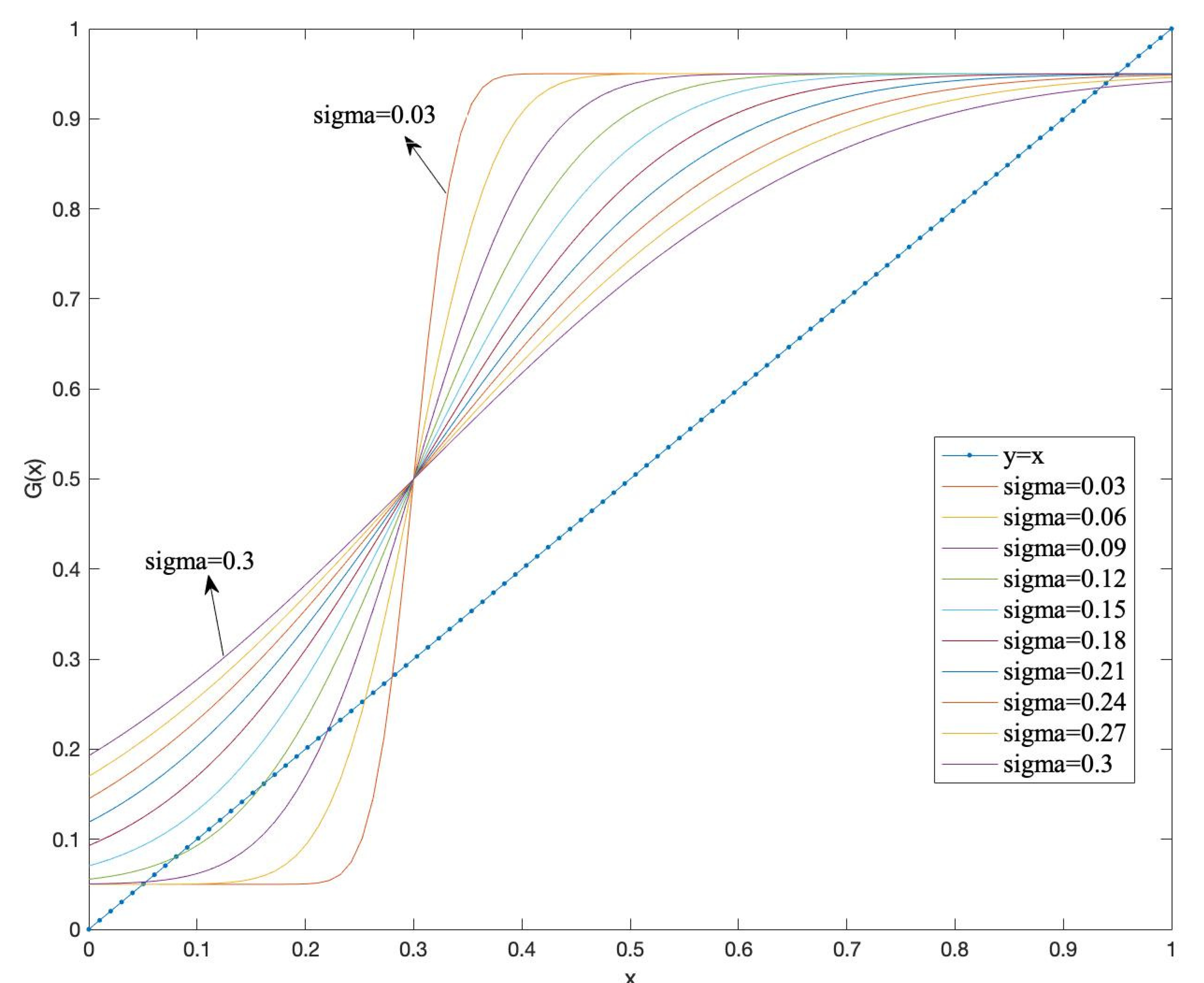
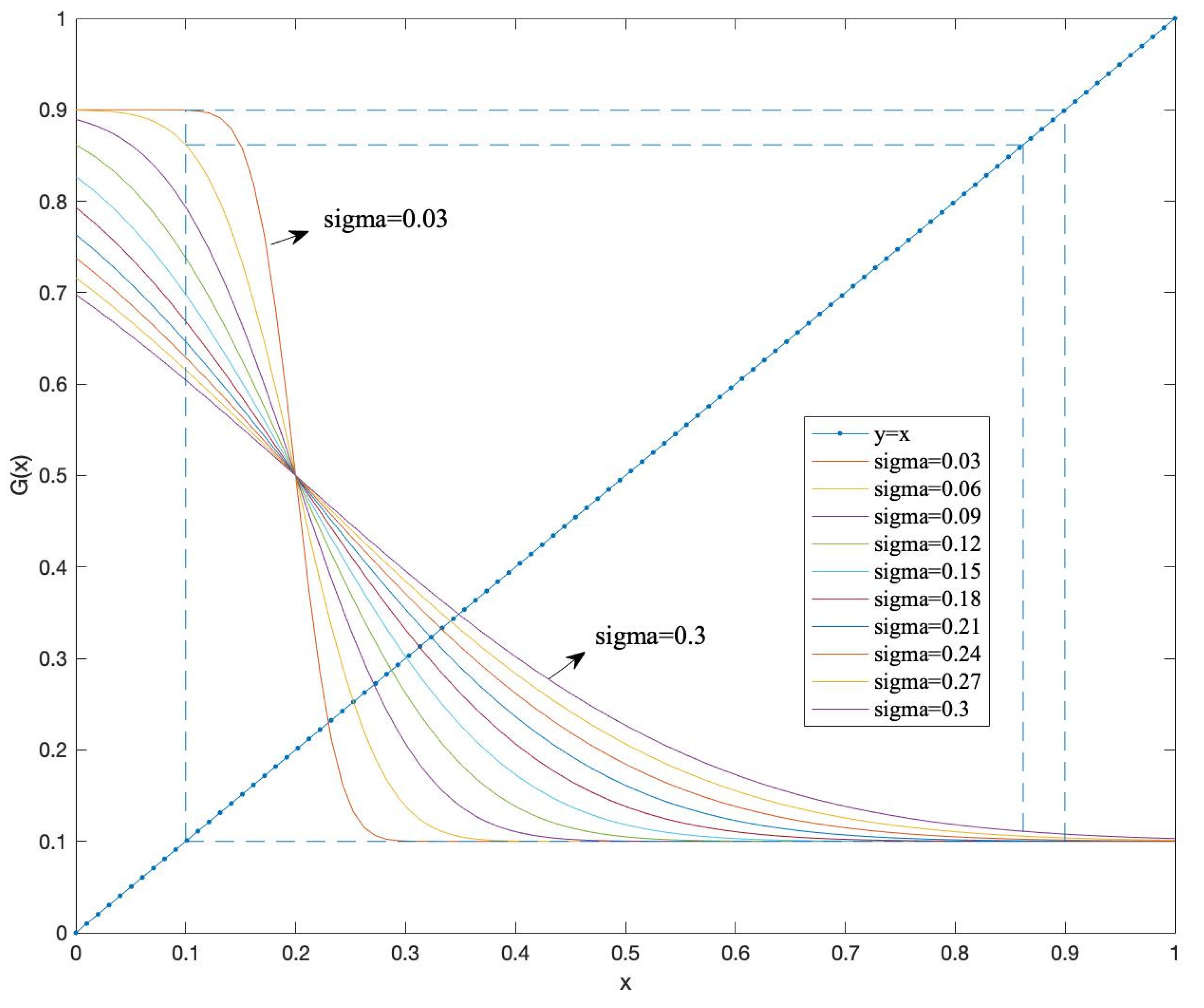
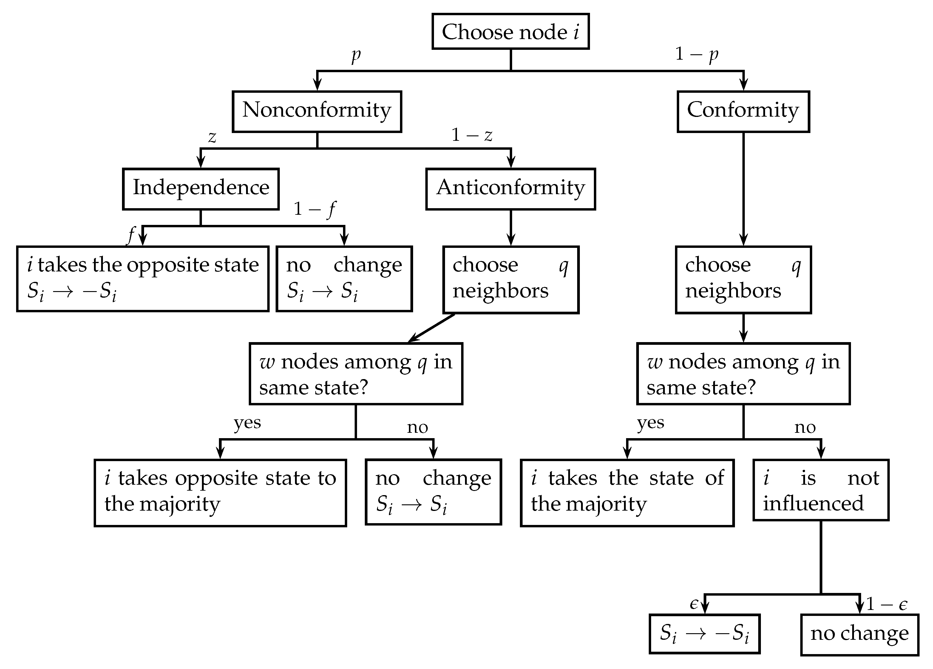
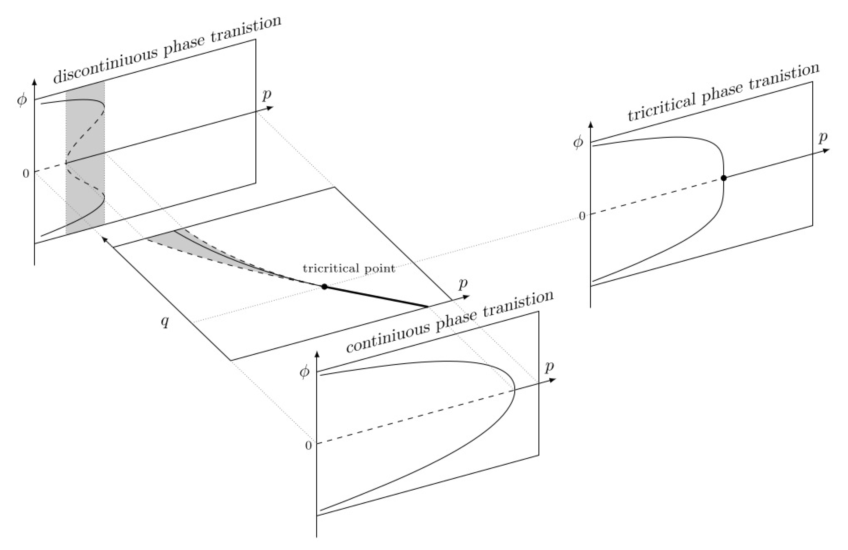
Table 1.
Summary of the main properties of the various models. disc. = discrete, cont. = continuous, sync. = synchronous, async. = asynchronous, conf. = conformist, anticonf. = anticonformist. Only most typical convergence results are indicated.
Table 1.
Summary of the main properties of the various models. disc. = discrete, cont. = continuous, sync. = synchronous, async. = asynchronous, conf. = conformist, anticonf. = anticonformist. Only most typical convergence results are indicated.
| Model | Opinion | Time | Updating | Behavior | Convergence | Other |
|---|---|---|---|---|---|---|
| Threshold | disc. | disc. | sync. | conf/anticonf | stable/unstable steady state/cycle | |
| q-voter | disc. | disc. | async. | conf/anticonf | stable/unstable steady state | |
| majority rule | disc. | disc. | async. | conf/anticonf | stable/unstable steady state | |
| aggregation | dis. | disc. | sync. | conf/anticonf | polarization, cycles, fuzzy polar., fuzzy cycles | |
| DeGroot | cont. | disc. | sync. | conf. | consensus | |
| Abelson | cont. | cont. | sync. | conf. | consensus | |
| Friedkin-Johnsen | cont | disc. | sync. | conf. | strong diversity | |
| Taylor | cont. | cont. | sync. | conf. | strong diversity | |
| Altafini | cont. | disc. | sync. | conf/anticonf links | polarization | |
| EPO | cont. | disc. | sybc. | conf. | strong diversity | private/public opinion |
| DeMarzo et al. | cont. | disc. | sync. | conf. | consensus | time-varying |
| Hegselmann- Krause | cont. | disc. | sync. | conf. | clustering | time-varying; bounded confidence |
Publisher’s Note: MDPI stays neutral with regard to jurisdictional claims in published maps and institutional affiliations. |
© 2020 by the authors. Licensee MDPI, Basel, Switzerland. This article is an open access article distributed under the terms and conditions of the Creative Commons Attribution (CC BY) license (http://creativecommons.org/licenses/by/4.0/).
Share and Cite
MDPI and ACS Style
Grabisch, M.; Rusinowska, A. A Survey on Nonstrategic Models of Opinion Dynamics. Games 2020, 11, 65. https://0-doi-org.brum.beds.ac.uk/10.3390/g11040065
AMA Style
Grabisch M, Rusinowska A. A Survey on Nonstrategic Models of Opinion Dynamics. Games. 2020; 11(4):65. https://0-doi-org.brum.beds.ac.uk/10.3390/g11040065
Chicago/Turabian StyleGrabisch, Michel, and Agnieszka Rusinowska. 2020. "A Survey on Nonstrategic Models of Opinion Dynamics" Games 11, no. 4: 65. https://0-doi-org.brum.beds.ac.uk/10.3390/g11040065
Note that from the first issue of 2016, this journal uses article numbers instead of page numbers. See further details here.