Cartel Formation in Cournot Competition with Asymmetric Costs: A Partition Function Approach


School of Political Science and Economics, Waseda University, 1-6-1, Nishi-waseda, Shinjuku-ku, Tokyo 169-8050, Japan
Games 2021, 12(1), 14; https://0-doi-org.brum.beds.ac.uk/10.3390/g12010014
Submission received: 11 December 2020
/
Revised: 6 January 2021
/
Accepted: 18 January 2021
/
Published: 1 February 2021
(This article belongs to the Special Issue Behavioral Coalition Formation: Theory and Experiments)
Abstract
:In this paper, we use a partition function form game to analyze cartel formation among firms in Cournot competition. We assume that a firm obtains a certain cost advantage that allows it to produce goods at a lower unit cost. We show that if the level of the cost advantage is “moderate”, then the firm with the cost advantage leads the cartel formation among the firms. Moreover, if the cost advantage is relatively high, then the formed cartel can also be stable in the sense of the core of a partition function form game. We also show that if the technology for the low-cost production can be copied, then the cost advantage may prevent a cartel from splitting.
JEL Classification:
C71; L131. Introduction
Many approaches have been proposed to analyze cartel formation. Ref. [1] first introduced a simple noncooperative game to study cartel formation among firms. As shown by the title of his paper, “A simple model of imperfect competition, where 4 are few and 6 are many”, this result suggests that cartel formation depends deeply on the number of firms in a market. Ref. [2] distinguished the issue of cartel stability from that of cartel formation. They focused on firms’ profits at an equilibrium and analyzed the stability of a cartel. Ref. [3] introduced the notion of a coalition-proof Nash equilibrium to analyze cartel stability. She defined a coalition-proof stable cartel and showed that there is a unique coalition-proof equilibrium. Ref. [4] analyzed cartel formation from a dynamic point of view. They showed that their dynamic process converges to a stable cartel if any.
In contrast to the approaches listed above, Ref. [5] uses a partition function form game to study an endogenously stable coalition structure in Cournot competition. Ref. [6] also formulates Cournot competition (and many other economic situations) as a partition function form game and focuses on the effects of positive/negative spillovers among firms. Our approach belongs to this group: we use a partition function form game. However, the following three features distinguish our approach from those of the preceding papers.
- We consider stable coalition structures. Although we will elaborate later, a coalition structure is a partition of a player set. Therefore, our analysis includes a situation where multiple cartels can coexist simultaneously.
- We use the concept of a core allocation to define the stability of a coalition structure. For each coalition structure, we assume that the members of each cartel divide their profit among themselves. We say a coalition structure is stable if there exists a feasible core allocation in the coalition structure.
- We introduce asymmetric costs and attempt to solve the so-called “merger paradox”. More specifically, we consider that a firm obtains new technology and a cost advantage that allow the firm to produce goods at a lower unit cost. We perform comparative statics for .
Intuitively, to understand the model, we consider a simple example with three firms. The firms produce homogeneous divisible goods. Let be an inverse demand function, where Q is the total amount of goods in this market. We first consider symmetric costs: all firms produce goods at a fixed unit cost c. For simplicity, we assume . Since there are three firms, by standard calculations, each firm obtains profit . Note that if there are n firms, in general, each firm obtains . We now focus on firms 1 and 2. We suppose that they decide to merge and form their coalition, or a cartel, . The two firms in the coalition jointly produce goods at the same unit cost c. Therefore, the market now consists of the two-firm coalition and firm 3. By the same calculations, the two-firm coalition obtains profit () in total. However, it immediately holds that , which means that the merger does not necessarily lead to a profit for both firms 1 and 2. To be more precise, at least one firm decreases its profit and, hence, has no incentive to join such a coalition. This phenomenon is known as the “merger paradox” in Cournot competition. According to this standard model, firms may have no incentive to form their coalitions, while many cartels are reported in our actual market.1
We attempt to address this problem in terms of cost asymmetry, coalition structure, and the core. We now assume that firm 1 obtains a cost advantage . Firm 1 produces goods at a lower unit cost . Let . Note that since . We assume that a coalition that contains firm 1 can enjoy the cost advantage and produces goods at the lower unit cost . We compute each coalition’s profit in every partition and obtain Table 1.2 In the table, firms j and k mean the symmetric firms 2 and 3.
We focus on the merger of firm 1 and firm 2 again. If coalition ’s joint profit is greater than the summation of firm 1’s profit and firm 2’s profit , then they have an incentive to merge.3 This inequality holds if and only if . Note that can take any nonnegative real number. In other words, if the level of the cost advantage of firm 1 is “moderate” (namely, ), then firm 1 profits by merging with firm 2. If the cost advantage is slight (namely, ), such a small advantage is almost negligible and not enough for both firms to improve their profits. If the cost advantage is very large (namely, ), firm 1 no longer needs to merge with firm 2: it is more profitable for firm 1 to produce goods alone by taking advantage of the very low cost. The latter two cases still suggest the merger paradox in two different ways, while the first case suggests the possibility of endogenous cartel formation. Moreover, as long as retains the moderate level , coalition also has an incentive to absorb firm 3 and form the three-firm cartel. Firm 3 also benefits by participating in this cartel.
Given this observation, one might have the following two questions. (i) Is this observation available for any number of firms? (ii) Are the formed cartels stable? The first question may arise from the simple fact that a coalition’s profit depends on the coalition structure in which the coalition is embedded. For example, in view of Table 1, even in the symmetric setting, firm 1’s profit is 1/16 if the other two firms are separate, while it is 1/9 if they form a two-firm coalition. The second question arises from the gap between cartel formation and cartel stability. As the preceding papers show, to analyze stable coalition structures, we need to take into account the profit distributions in each coalition. For example, we focus on partition in the asymmetric setting. In view of Table 1, firm 3 simply obtains alone, while firms 1 and 2 must negotiate and divide the profit . Given that firm 1 might be in an advantageous position because of its cost advantage, how do they distribute the profit to keep their coalition? As mentioned in question (i), this problem becomes more complicated if we consider n firms and all possible partitions of the n firms. We employ a partition function form game to address these difficulties. All the propositions that we provide in this paper hold for any n. Moreover, we apply the core of a partition function form game to discuss stable coalition structures.
To provide the formal framework, we introduce basic notation in Section 2. We discuss cartel formation in Section 3 and cartel stability in Section 4. In Section 5, we extend the basic model so that a firm can copy the technology to produce goods at the low unit cost. We summarize the results in Section 6. All the proofs are provided in the Appendix A.
2. Preliminaries
Let be a set of firms. Throughout this paper, we assume . Let S be a coalition of firms: . By , we denote the cardinality of coalition S, namely, the number of firms in coalition S. We typically use to denote a partition. Let be the set of all partitions of coalition S. We denote the number of coalitions in partition by . An embedded coalition is with and . Let be the set of all embedded coalitions of N. A partition function v assigns a real number to each embedded coalition, . A partition function form game is a pair .
The framework of Cournot competition is the same as the one we mentioned in Section 1. The firms produce homogeneous goods. They are free to form coalitions among themselves. Let
be an inverse demand function, where Q is the total amount of products in this market, . We first briefly introduce a symmetric setting as a benchmark. Every firm produces output at a fixed unit cost c. For simplicity, we assume
We obtain a partition function form game in the same manner as Section 1 (see Table 1): for every , we have
Now, we suppose that a firm, for example, firm 1, obtains a cost advantage . Let be the new unit cost of firm 1, namely,
where let . As long as a coalition contains firm 1, the coalition can enjoy the cost advantage and produces goods at the lower cost . The following proposition provides the partition function in the presence of the cost advantage .
Proposition 1.
Let . For any ,
Proposition 1 allows us to use the following simple notations. First, for any , let
We use to denote the profit of the coalition containing firm 1. By , we denote the profit of a coalition with the standard cost. Formally,
Therefore, each coalition’s profit depends on a nonnegative real number and a natural number .
3. Cartel Formation
The partition function provided in Proposition 1 specifies “which coalition obtains how much profit in which coalition structure” in the presence of the cost advantage of firm 1. The following result shows that any coalition that consists of firms with the standard cost has an incentive to split. Moreover, this disintegrative tendency holds for any .
Proposition 2.
For any and any ,
Note that means (the number of coalitions in) the coalition structure after the split, and means that before the split. The right-hand side, , means the summation of the profits of the (sub)coalitions, say, T and , that belonged to the same coalition, say, , before the split. Therefore, this proposition states that regardless of what profit distribution is made in the original coalition S, either T or has an incentive to deviate from S. The inequality is required because if , then either one of the two coalitions contains firm 1, and this proposition does not apply.4
Proposition 2 also suggests that the merger paradox persists among the firms with the standard cost. Who leads cartel formation? The following proposition answers this question.
Proposition 3.
For any and any , let
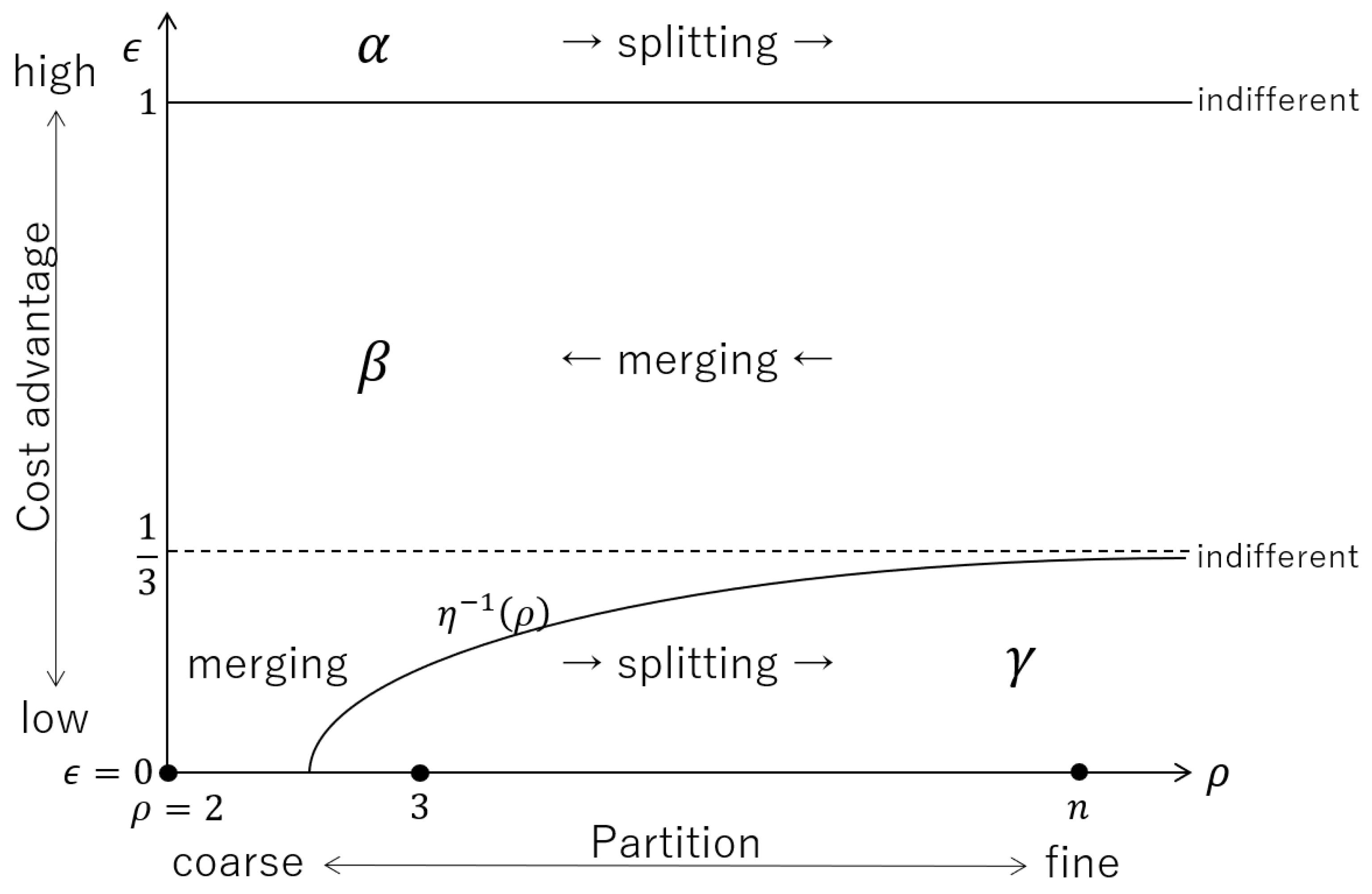
For the sign of , Table 2 holds, where for , and m denotes the gains from cooperation.
For example, if , is negative for every with . Similarly, if and , then is positive. If is positive, then both the coalition containing firm 1 and a coalition without firm 1 have an incentive to merge into one large coalition. In contrast, if it is negative, either one of them has an incentive to deviate from the large coalition. If zero, they are indifferent between merger and split. Figure 1 describes this relationship. Note that for , we have
and .
We can derive the following three implications from Proposition 3 and Figure 1.
- As shown in the area , if the level of the cost advantage is “moderate”, firm 1 obtains an incentive to lead coalition formation. Moreover, as long as retains the moderate level, each merger benefits all participants.
- The area shows that if the cost advantage is slight and if there are three or more coalitions, then such an advantage is too small for firm 1 to lead cartel formation. In this case, the symmetric setting and the asymmetric setting are hardly different.
- In contrast, if the cost advantage is very large as the area describes, then such “strong” firm 1 no longer needs any cartel. Firm 1 has an incentive to be alone and produce goods by taking full advantage of the very low unit cost.
Moreover, by combining Propositions 2 and 3, we can depict the flow of splits and mergers among firms. To demonstrate this, we provide the following four-firm example.
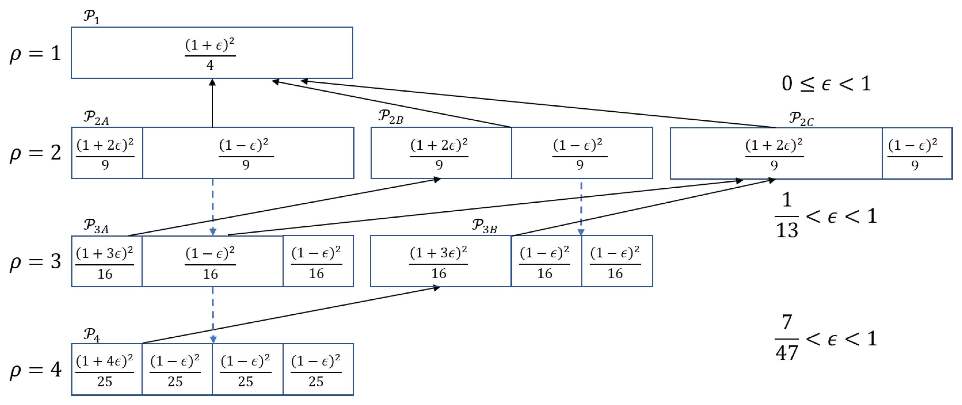
Example 1.
We consider four firms, . Set partitions as follows: for ,
These partitions cover all possible coalition structures of the four firms. Figure 2 shows the splits and mergers among these firms. The three dashed downward arrows are derived from Proposition 2. Therefore, these three arrows hold for any . Proposition 3 generates the upward arrows with continuous lines. These upward arrows are conditional. Since , the maximum of ρ is 4. If ϵ satisfies , then all the upward arrows are valid. However, if ϵ is in , the arrow from to would point downward. The two upward arrows from and to are valid as long as ϵ is less than 1. If ϵ exceeds 1, all arrows would point downward.
We now focus on a sequence of splits and mergers. For example, we consider . Let ϵ satisfy : all arrows in Figure 2 are valid. In particular, three arrows are available from partition . Regardless of which arrow one follows, there is a sequence of mergers that reaches . All partitions, including , have such a sequence.
This observation generalizes to any number of players. Proposition 3 implies the following result.
Corollary 1.
For any , there exists ϵ such that for every partition , we can find a sequence of two-coalition mergers that starts from and reaches .
Figure 2, together with Corollary 1, suggests that the grand coalition can be formed if . However, as we mentioned in Section 1, forming a coalition structure does not necessarily mean that the coalition structure is stable. Its stability depends on the profit allocation the firms decide within the coalition. In Section 4, we provide a condition for coalition structures to be (un)stable. Proposition 4 is the formal statement that covers all coalition structures of n firms. Figure 3 shows the application of Proposition 4 to the four-firm case.
4. Cartel Stability
A cartel obtains profit from Cournot competition and distributes the profit among its members. If some members object to the profit distribution, the members may deviate from the cartel and form their own coalition. Firms may negotiate on their distribution before forming their cartel. In the negotiation, if a proposed allocation is profitable for all members of the coalition, then they form the coalition, and the resulting coalition should be stable. However, if it is not profitable for some firms, they have no incentive to agree to such a distribution and will not join the cartel. In this sense, we need to analyze profit distributions to study stable coalition structures. We use the stability concept known as the core. We begin with the definition of the core for a partition function from game.5
Let . For each partition , the set of feasible allocations is given as follows: , where the definition of is given in Proposition 1. In other words, every coalition in a partition distributes its profit within the coalition. Now, we define a deviation. To define a deviation in a partition function form game, we briefly introduce some useful notations. For any , let be the projection of partition on coalition S, formally . Hence, is the partition of S such that reserves the partition of N by . For example, if and , then . For simplicity, define
Therefore, for the same S and , , which is the partition that results after the members of S leave partition and form their own coalition S. For any and any , a coalition S deviates from x if there exists such that for every .6 The core for partition is the set of feasible allocations from which no coalition deviates:
and we say a partition is stable if the core of the partition is nonempty.
The following proposition shows the relationship between the cost advantage and the nonemptiness of the core. We define the following number, which serves as a threshold in the proposition:
Note that is assumed throughout this paper, and we have for every .
Proposition 4.
Let . If ϵ satisfies , then is empty for every . Moreover, for the grand coalition N,
Together with Corollary 1, this proposition suggests the following:
- As long as the cost advantage is in the “moderate” interval , Corollary 1 suggests that firm 1 leads coalition formation and reaches the grand coalition N.
- Moreover, if lies in the particular interval , then the grand coalition that is achieved is stable. No coalition has an incentive to deviate from the grand coalition.
- However, if is in , the formation of the grand coalition is transient because every allocation in the grand coalition is not a core allocation. Some coalitions endogenously deviate from the grand coalition.
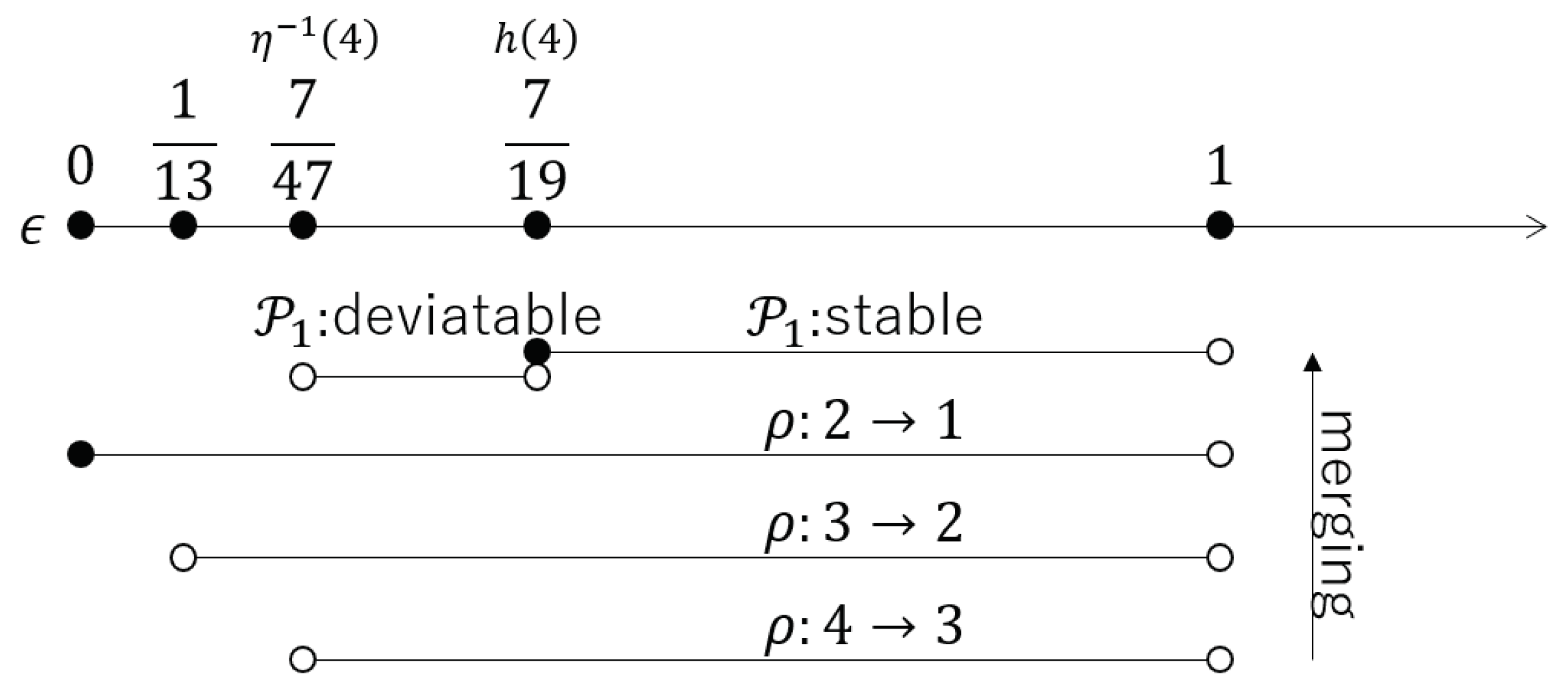
Below, we apply Proposition 4 to the four-firm example. Since , we have
For any with , all upward arrows (and all dashed arrows) are valid in Figure 2. In this sense, as Corollary 1 states, the grand coalition N is reachable from every coalition structure. The threshold is given as
Figure 3 summarizes the intervals. If cost advantage lies in the most strict interval , the grand coalition can be seen as the “goal” of a sequence of splits and mergers because there is a core allocation in the grand coalition, from which no coalition deviates. To check the existence of core allocations, we consider two levels of cost advantages: low and high . First, let . The four firms divide the total profit among themselves.7 Firm 1 requires at least because firm 1 can attain this profit by deviating from the grand coalition and forming its one-firm coalition. Similarly, firm 2 requires at least . Firms 3 and 4 also require the same amount as firm 2. However, we have
Hence, for any feasible allocation, at least one firm has an incentive to deviate, which means the grand coalition is also a transient step of the sequence. Now, let . The four firms divide the total profit among themselves.8 The grand coalition now has a core allocation. For example, allocation becomes a core element. Therefore, no coalition deviates from this allocation.
In view of the first and second points of the three implications listed above, one might consider that “reaching the grand coalition” and “reaching a core element of the grand coalition” can be different. Although they are different in general, we can straightforwardly remove this gap in our model. To see this, we construct a sequence of allocations that reaches a core element of the grand coalition. We demonstrate this below. Let .
We consider the sequence of partitions and the sequence of allocations as follows:9
This sequence meets the following three requirements: (i) allocations are monotonically increasing; (ii) allocations are feasible in each step; and (iii) the final allocation lies in the core. The first requirement is known as population monotonicity, which guarantees all firms an incentive to form a larger coalition.10
5. The Spread of Technology
In the previous sections, we assumed that the cost advantage and the technology belonged solely to firm 1 and that any firm could not copy the technology. In this section, we assume that if a firm forms a coalition with firm 1, then the firm can make use of the technology, even after the firm becomes independent from the coalition.
To describe the situation, we use the four-firm example again. We consider partition to be the first step. In this step, firm 1 is still the only firm that has the technology. Now, firm 1 and firm 2 form their coalition and move to the partition . In this step, firm 2 learns the technology from firm 1. Firm 2 does not have to use the technology in partition because firm 2 can enjoy the full technology, as long as it keeps a coalition with firm 1. However, firm 2 can use the technology to some degree even after it splits off from the coalition. We use r to denote the degree of availability of the technology. In other words, if firm 2 splits off from the coalition, firm 2 can produce goods at a new unit cost , where . It holds that . If , firm 2 can make full use of the technology, . If , the technology is completely protected by firm 1, and firm 2 cannot use it at all, . Note that no firm can use the technology until it goes through the coalition with firm 1.
Since we have already analyzed the case with in the previous sections, we now observe the other extreme case . Suppose firm 2 splits off from the coalition and moves from to . Firms 1 and 2 are symmetric in with the lower cost . Firms 3 and 4 are also symmetric in with the higher cost c. Therefore, each firm obtains the following profits in :
where the third input 1 means . We use to denote the profits in the “second” , in which firm 2 also has the cost advantage, and to write those in the “first” , in which firm 2 did not have the cost advantage.
Now, we focus on the difference between and . If , as we have seen in the previous sections, the deviation from to is not necessarily profitable for firm 2 because as long as satisfies , it holds that
as described in Figure 2. However, if , for any , we have
This observation means that each firm’s incentive to form and dissolve a coalition depends on the level of r.
The natural question should be what r facilitates the splits and mergers of coalitions. To answer this question, we introduce some notations below. They are a formal version of the observation provided above. Let . Consider a coalition with and . Fix a partition with . Let and satisfy , , and . Let be the partition that results after either or splits off from . Therefore, coalition can produce goods at unit cost in partition . Let denote the profit of in partition , and be that of . In the same manner as Proposition 1, we have
We use to denote the profit of coalition T for each T in . Note that since .
Proposition 5.
Let and . The following two statements are equivalent:
- (i)
- There is such that
- (ii)
- It holds that .
If , statement (i) holds for any .
Note that statement (ii) means that pair lies in either or in Figure 1. Therefore, the existence of r as mentioned in statement (i) distinguishes the areas and , in which firms tend to split. If is in , some r prevents splits, while if it is in , no r prevents splits. To see this, we use the four-firm example and consider the partitions and . We focus on firm 1 and firm 2. In view of (2) and (1), their profits are given as follows:
First, we consider a high cost advantage , so is in . We set, for example, . We have
Hence, this r prevents the coalition from splitting. However, if is so small that it is in the area , no r prevents the split. For example, consider . Then, the opposite inequality holds for every r. Why does such r exist only in ? The area means that firm 1’s cost advantage is very high. Therefore, if r is zero, then firm 1 has an incentive to form its one-firm coalition, as discussed in Proposition 3. Even if r is positive, as long as r is small, the result is the same as .11 However, if r is high enough, such r also gives firm 2 an incentive to deviate together with the “partial” cost advantage , which discounts the original advantage of firm 1. To prevent firm 2 from splitting off, firm 1 assigns more shares to firm 2. As long as firm 1 serves firm 2 satisfactory share, their coalition does not split. If r is very high or one, then firm 2 can expect even higher profit after the deviation. In this case, firm 1 is no longer able to offer enough share for firm 2, and their coalition splits.
If it is in the area , is very slight, and is even slighter. Such a small advantage no longer influences any firm’s incentive. Therefore, the behavior of firms is the same as in the case with .
6. Concluding Remarks
In this paper, we have employed a partition function form game to formulate cartel formation among firms in Cournot competition. We have shown that the result of cartel formation depends on the level of the cost advantage a firm attains. If the level of the cost advantage lies in a certain interval, the firm that has the cost advantage obtains an incentive to lead cartel formation and reach the grand coalition. Moreover, if the cost advantage level is in a more restrictive interval, that is, a subinterval of the above interval for coalition formation, then the grand coalition that has been achieved can also be stable in the sense of the core. In addition, we have shown that if the technology for the cost advantage can be copied, then such technology may prevent cartels from splitting.
Throughout this paper, we have assumed that the level of the cost advantage, , is constant. However, the technology can develop as mergers proceed. For example, in view of Figure 1, starting from a certain level of in the area , may increase as mergers proceed and exceed 1 at some point. According to the area , such a high level of technology now facilitates splits. If the technology can be copied, the developed technology spreads in the market as firms split up. As a result, the developed technology spreads over many firms in the market, which may result in symmetric costs with the new technology. If a firm obtains another technology in the state and the costs become asymmetric again, then a new sequence of mergers and splits may start. Further research is required to extend the model to incorporate such a dynamic change in .
Funding
This research was funded by JSPS Grant-in-Aid for Research Activity Start-up (No. 19K23206) and Waseda University Grant-in-Aid for Research Base Creation (2019C-486). The APC was funded by Waseda University (School of Political Science and Economics).
Institutional Review Board Statement
Not applicable.
Informed Consent Statement
Not applicable.
Data Availability Statement
No new data were created or analyzed in this study. Data sharing is not applicable to this article.
Conflicts of Interest
The funders had no role in the design of the study; in the collection, analyses, or interpretation of data; in the writing of the manuscript, or in the decision to publish the results.
Appendix A
Appendix A.1. Proof of Proposition 1
Proof.
We fix a partition . Let be a profile of quantities produced by the coalitions in . We use to denote the coalition that contains firm 1. By S, we denote a coalition that does not contain firm 1. We first consider the best response function of coalition . Coalition S’s profit is . Hence, the best response function of coalition S is
In the same manner, since coalition ’s profit is given as , we have
Given the coalitions except are symmetric, we solve these equations and obtain the following equilibrium quantities:
Hence, the equilibrium profits are
□
Appendix A.2. Proof of Proposition 2
Proof.
For any , we have
□
Appendix A.3. Proof of Proposition 3
Proof.
For any and any , we have
Let . It holds that for any . Since this is increasing with respect to , and we have
we obtain for every . If , then clearly for every .
Let . If , then it follows that for every . Since is also negative, we have for any . Now let . For any with , we have
Set . For , is increasing. Moreover, we have
Hence, for any with , we have:
for ; for ; and for .
This completes the proof. □
Appendix A.4. Proof of Proposition 4
Proof.
Let . We first show that for every the core of becomes empty. We fix . Assume that there exists . Let be the coalition that satisfies . Since , there is a coalition in that is different from . We call it . Now we consider their union and partition . Note that and .
Moreover, since function is monotonically increasing, we have . Hence, in view of the first constraint , it holds that , where the left inequality means for since is bijective on the domain . In addition, we have because . Hence, it follows from Proposition 3 that
We define y as follows: for every ,
and, for the other players, set to satisfy
Below we show . First, implies , which means
Now, for the coalition , we have
Moreover, for every , we have
Hence, coalition deviates from x, which contradicts . Thus, is empty.
Now we focus on the partition . We first let . Assume that there exists . For every player , it holds that . Hence,
For every player , we have
In the same manner, for the player 1,
Since , any one-person coalition does not deviate from x, which implies
Since ,
Hence, the inequality (A6) holds if
Hence, if violates this condition (namely, if ), then at least one player has an incentive to deviate from x, which means is empty. If , then there exists an allocation such that no one-person coalition deviates from . In view of Proposition 1, for any , is independent from the cardinality of S. Hence, no coalition deviates from , namely, . □
Appendix A.5. Proof of Proposition 5
Proof.
The inequality of the first statement is equivalent to
The formula in the parenthesis is equal to
This is equal to or greater than zero if and only if
where always holds for every .
Let . For every , it holds that
Hence, we consider the condition that establishes
This inequality holds if and only if
Hence, some r satisfying (A7) exists in if and only if .
References
- Selten, R. A simple model of imperfect competition, where 4 are few and 6 are many. Int. J. Game Theory 1973, 2, 141–201. [Google Scholar] [CrossRef] [Green Version]
- D’Aspremont, C.; Jacquemin, A.; Gabszewicz, J.J.; Weymark, J.A. On the stability of collusive price leadership. Can. J. Econ. 1983, 16, 17–25. [Google Scholar] [CrossRef] [Green Version]
- Thoron, S. Formation of a coalition-proof stable cartel. Can. J. Econ. 1998, 31, 63–76. [Google Scholar] [CrossRef] [Green Version]
- Kuipers, J.; Olaizola, N. A dynamic approach to cartel formation. Int. J. Game Theory 1983, 37, 397–408. [Google Scholar] [CrossRef] [Green Version]
- Ray, D.; Vohra, R. A theory of endogenous coalition structures. Games Econ. Behav. 1999, 26, 286–336. [Google Scholar] [CrossRef] [Green Version]
- Yi, S.S. Stable coalition structures with externalities. Games Econ. Behav. 1997, 20, 201–237. [Google Scholar] [CrossRef]
- Salant, S.W.; Switzer, S.; Reynolds, R.J. Losses from horizontal merger, The effects of an exogenous change in industry structure on Cournot-Nash equilibrium. Q. J. Econ. 1983, 98, 185–199. [Google Scholar] [CrossRef] [Green Version]
- Artz, B.; Heywood, J.S.; McGinty, M. The merger paradox in a mixed oligopoly. Res. Econ. 2009, 63, 1–10. [Google Scholar] [CrossRef]
- Abe, T.; Funaki, Y. The non-emptiness of the core of a partition function form game. Int. J. Game Theory 2017, 46, 715–736. [Google Scholar] [CrossRef]
- Abe, T. Consistency and the core in games with externalities. Int. J. Game Theory 2018, 47, 133–154. [Google Scholar] [CrossRef]
- Bloch, F.; van den Nouwel, A. Expectation formation rules and the core of partition function form games. Games Econ. Behav. 2014, 88, 339–353. [Google Scholar] [CrossRef]
- Kóczy, L.Á. A recursive core for partition function form games. Theory Decis. 2007, 63, 41–51. [Google Scholar] [CrossRef] [Green Version]
- Yang, G.; Sun, H.; Hou, D.; Xu, G. Games in sequencing situations with externalities. Eur. J. Oper. Res. 2019, 278, 699–708. [Google Scholar] [CrossRef]
- Hart, S.; Kurz, M. Endogenous formation of coalitions. Econometrica 1983, 51, 1047–1064. [Google Scholar] [CrossRef]
- Kóczy, L.Á. Partition function form games. In Theory and Decision Library C 48; Springer International Publishing: Cham, Switzerland, 2018. [Google Scholar]
- Sprumont, Y. Population monotonic allocation schemes for cooperative games with transferable utility. Games Econ. Behav. 1990, 2, 378–394. [Google Scholar] [CrossRef]
- Abe, T. Population monotonic allocation schemes for games with externalities. Int. J. Game Theory 2020, 49, 97–117. [Google Scholar] [CrossRef]
- Abe, T.; Liu, S. Monotonic core allocation paths for assignment games. Soc. Choice Welf. 2019, 53, 557–573. [Google Scholar] [CrossRef]
| 1. | Ref. [7] discusses the merger paradox in a simple framework: In their model, a merger of firms, in most cases, generates a decline of the joint profits, while, in our settings that are formally introduced later, we assume that a firm obtains cost advantage, and the cost asymmetry gives the firm an incentive to merge with other firms. Moreover, asymmetric settings are also studied by Ref. [8]. They consider a mixed oligopoly that consists of private firms and a public firm. They show that there is a merger between a private firm and the public firm that may benefit the members of the merger. |
| 2. | For example, in partition , firm 1 with the lower unit cost and firms 2 and 3 with the standard unit cost c compete under the same inverse demand function. |
| 3. | There is a profit distribution that improves both firms’ profits. |
| 4. | Note that means the profit of a coalition with the standard cost. |
| 5. | |
| 6. | One can define a deviation in another way: for every and for some . These two definitions make no difference in the following results. |
| 7. | For easy reference, we provide the list of profits for . Below, means the coalition that contains firm 1, and S means a coalition without firm 1: ; , ; , ; , . |
| 8. | Below is the list of profits for : ; , ; , ; , . |
| 9. | The denominator 14,400 is the LCM of 16, 9, 36, 64, 25, and 100. |
| 10. | For a detailed discussion of population monotonicity, see the following papers. A sequence of population monotonic allocations is called a population monotonic allocation scheme (PMAS). This concept was formally introduced by [16], and Ref. [17] studied conditions for a partition function form game to have a PMAS. Ref. [18] weakens some restrictions of PMAS and propose a monotonic core allocation path (MCAP). |
| 11. | To be more precise, as elaborated in (A7) in the Appendix A, r is “small” if it is less than , and “high enough” if it lies between and , and “very high” if it exceeds . |
Figure 1.
Cost advantage and tendency of coalition formation.

Figure 2.
Splits and mergers among four firms.

Figure 3.
Cost advantage, stability, and cartel formation among four firms.


Table 1.
Profits in Cournot competition with three firms.
| Partition | {{1},{2},{3}} | {{1,j},{k}} | {{2,3},{1}} | |||||
|---|---|---|---|---|---|---|---|---|
| Coalition | ||||||||
| Symmetric costs | ||||||||
| Cost advantage | ||||||||
Table 2.
The sign of .
| negative | |||
| zero | |||
| positive | |||
| positive | zero | negative | |
| if | if | if |
Publisher’s Note: MDPI stays neutral with regard to jurisdictional claims in published maps and institutional affiliations. |
© 2021 by the author. Licensee MDPI, Basel, Switzerland. This article is an open access article distributed under the terms and conditions of the Creative Commons Attribution (CC BY) license (http://creativecommons.org/licenses/by/4.0/).
Share and Cite
MDPI and ACS Style
Abe, T. Cartel Formation in Cournot Competition with Asymmetric Costs: A Partition Function Approach. Games 2021, 12, 14. https://0-doi-org.brum.beds.ac.uk/10.3390/g12010014
AMA Style
Abe T. Cartel Formation in Cournot Competition with Asymmetric Costs: A Partition Function Approach. Games. 2021; 12(1):14. https://0-doi-org.brum.beds.ac.uk/10.3390/g12010014
Chicago/Turabian StyleAbe, Takaaki. 2021. "Cartel Formation in Cournot Competition with Asymmetric Costs: A Partition Function Approach" Games 12, no. 1: 14. https://0-doi-org.brum.beds.ac.uk/10.3390/g12010014
Note that from the first issue of 2016, this journal uses article numbers instead of page numbers. See further details here.