
Coordinating Carbon Emissions via Production Quantities: A Differential Game Approach

1
The Graduate School of Business Administration, Bar-Ilan University, Ramat Gan 5290002, Israel
2
Department of Industrial Engineering and Management, ORT Braude College, Karmiel 2161002, Israel
*
Author to whom correspondence should be addressed.
Games 2021, 12(1), 15; https://0-doi-org.brum.beds.ac.uk/10.3390/g12010015
Submission received: 17 December 2020
/
Revised: 19 January 2021
/
Accepted: 21 January 2021
/
Published: 3 February 2021
(This article belongs to the Special Issue Cooperation, Innovation and Safeguarding of the Environment)
Abstract
:Production emissions in the industrial sector are a major source of environmental pollution. In this paper, we explore how emission considerations are integrated with production decisions. We develop a dynamic model consisting of two firms located in the same industrial park, which satisfies exogenously given demands in separate markets. The two firms can build up or rundown stocks (full backlogging), both of which are costly. The emission cost depends on the total output of the two firms. We develop Nash equilibrium feedback strategies, where each firm decides on its output based on its inventory or the inventories of both. We also develop a social planning solution where decisions are centralized. We present the analytic results for the total profits in these settings. The results show the benefits of a decentralized approach over a centralized one, provided there is a mechanism for coordination. Finally, emission costs are compared for the various solution concepts.
1. Introduction and Literature Review
The industrial manufacturing sector consumes the lion’s share of the total consumption of electricity. In the Organisation for Economic Co-operation and Development (OECD) alone, electricity consumption in the industrial sector accounted for 32% in 2018 and accounted for 42% globally [1]. This global consumption figure is expected to exceed 50% by 2050 [2]. This constitutes an enormous burden to industry and makes up a considerable part of the total worldwide carbon emissions. Manufacturing and production activities are responsible for a massive part of the total emissions. For example, food production is responsible for 25% of the world’s greenhouse gas emissions [3]. Hence, any attempt to improve production activities by incorporating emission considerations into the decision-making process constitutes the right step forward.
Electricity providers use various technologies to produce electricity, each with a bounded capacity. These technologies range from those with minimal impact on the environment, e.g., dedicated wind parks and bio-mass electricity generators, to those with an obvious impact on the environment, e.g., conventional carbon-based technologies. Thus, electricity providers have an array of technologies at their disposal. Typically, a provider starts with the less expensive technology, and then once that capacity no longer suffices, it turns to the second least expensive one and so forth until the total capacity is met. However, environmental regulations have forced electricity providers to utilize newer technologies that are less polluting. In recent years, the electricity cost of renewable technologies, which are less polluting, has dropped, and in many cases is cheaper than coal [4]. Hence, as the total demand for electricity increases, the burden on the environment is likely to increase. Thus, frameworks and policies to control or mitigate the total quantities of emissions are critical.
A growing fraction of industrial activity today takes place in industrial parks, where a cluster of businesses engage in industrial activity in the same location [4,5]. Industrial parks do not only cover a major part of industrial activity, but also create a unique opportunity from a sustainability perspective [6]. Examples include District Heating (DH) and managing electricity consumption in micro-grids. Since heating is responsible for large amounts of energy consumption (in 2009, heating was 47% of the total energy consumption worldwide, [7]), centralized DH solutions have proven to be efficient in reducing CO2 emissions. Likewise, we posit that by coordinating the production of firms in an industrial park, we can reduce the amount of emissions they generate.
A micro-grid consists of several components: a carbon-emission-reduced generation method, such as a wind park, the industrial users of the park, and an independent load manager [8,9,10]. One practical approach considers that the industrial park can play a role in reducing the burden on the environment by influencing the production policies of the firms in the park. Initiatives that exemplify how energy consumption can be managed in a coordinated fashion to improve the performance can be found, for example, in [11].
The idea of controlling the impact of electricity generation on the environment is not limited to industrial parks. It can also be implemented on an individual basis, where a manufacturer utilizes an electricity pricing scheme to efficiently schedule operations so that the demand for electricity is leveled. The objective in this case is to minimize costs including electricity by leveling the peak-to-average ratio (see, e.g., [11]). Thus, coordinating energy consumption with operations, whether through scheduling or production planning, can lead to better and sustainable decisions, at least from the angle of lowering CO2 emissions whose negative impact on the environment has been amply demonstrated. This approach has been applied in a variety of settings, such as for electricity providers and retailers [12,13] and building electricity management [14,15,16]. Ref. [17] studied peak-load reduction for a manufacturing job scheduling problem, and [18] investigated peak-load reduction in a stochastic make-to-stock manufacturing setting.
Most operation management models for manufacturing or service operation policies assume constant operating costs, but in fact the impact of energy consumption on the environment is, by nature, far from being linear. Moreover, in most cases, studies have not considered the effects of production quantities on the level of carbon emissions (e.g., [19,20]). In this paper, we shed light on the relationship between these two and analyze the carbon emission with respect to the total production quantities. This is consistent with previous studies that have dealt with peak-load leveling; see, e.g., [20]. Ref. [21] was among the first to explicitly consider electricity prices in the management of a simple make-to-stock manufacturing facility with a base-stock policy.
In a deterministic setting, sustainability considerations have been incorporated with inventory in an Economic Order Quantity (EOQ) setting (e.g., [22,23,24,25,26]). However, this line of research only considers a single manufacturing facility and exogenously determined electricity prices. Other studies that have examined a game-theoretic setting, such as [27], have focused on a supplier-manufacturer setting.
In this paper, we analyze how incorporating the impact of electricity consumption into the total cost affects the production strategies of two manufacturers located in the same industrial park, who share the same sources of electricity. We investigate how carbon emissions and the total profitability of each manufacturer are affected by the level of coordination between the two firms. To take these into account, we evaluate the carbon emission costs as a function of the total sum of the production volumes of these two manufacturers, which allows for coordination between the two.
For that purpose, we compare the performances of the system in three scenarios: (1) a decentralized strategy depending on inventories, (2) a decentralized strategy depending solely on each firm’s own inventory, and (3) a centralized strategy. The decentralized strategies are coordinated via the production quantities of both firms. We develop the models and derive analytic results. The optimal production quantities and the optimal inventory levels are derived. Our results show that a decentralized approach with coordination performs better than a centralized strategy.
This paper is organized as follows: in Section 2 we present the model formulation and in Section 3, we analyze the model and obtain the analytic results. In Section 4, we conduct comparisons and in Section 5 we report the sensitivity analyses. We conclude and discuss the managerial implications and future directions in Section 6. All the technical proofs appear in the Appendix A.
2. Model Formulation and Notation
We consider an industrial park with two manufacturing units. Each manufacturing unit faces an exogenous market demand at an exogenous price. In order to produce electricity, the park’s energy management unit uses various types of technologies in a decreasing order of electricity production/supply costs. The level of carbon emission per unit of electricity consumed increases in the overall load of the industrial park, because, as mentioned earlier, renewable technologies are increasingly becoming cheaper than coal. Thus, the energy management unit can incentivize the firms to coordinate production quantities such that electricity consumption peak levels are leveled as much as possible. We describe a way to coordinate these decisions.
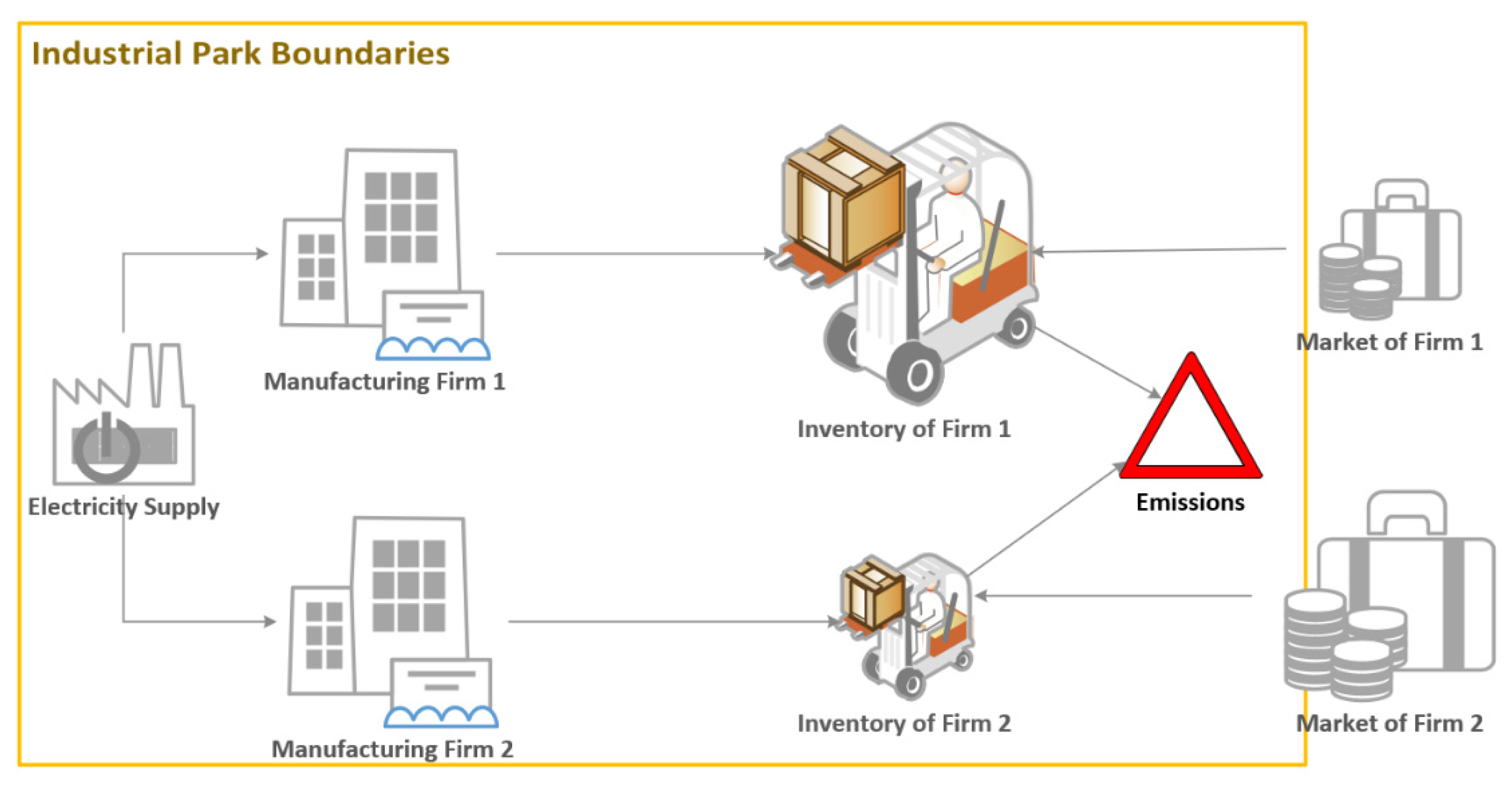
The manufacturing units decide on the production output that replenishes their inventories. In principle, the manufacturing units aim to supply the demand while reducing the carbon emissions associated with the quantities produced. This approach resonates with their overall sustainability business strategy. To control emission costs, each manufacturing unit is charged a penalty for the carbon emissions that stem from the production activity. Here we assume that this penalty pertains to the carbon emissions arising from the generation of the electricity consumed in the production of each unit produced by each manufacturing firm. In Figure 1, we depict the structure of this setting.
The production output qj(t) j = 1, 2, replenishes the inventory, whose dynamics can be captured by the following differential equation:
In (1), Ij(t) and Sj(t) represent the inventory and the sales rate of manufacturer j at time t, respectively, and Ij(0), is the initial inventory level. In this study we tackle the case where the demand rate is known and constant, which represents the best nominal (average) forecast for each firm for the foreseen horizon (e.g., [28]).
According to Equation (1), for manufacturing unit j, if the output rate is greater than the sales rate, then inventory is accumulated. If the opposite is true, then the inventory depletes. Thus, the inventory is a stock variable that measures the accumulated imbalance between quantities produced and demanded over time. A positive inventory level means that products are physically available, whereas a negative inventory level means that the company has outstanding backorders, i.e., we assume full backlogging.
The manufacturing units earn a positive margin from their sales but must pay a cost for holding positive inventory and for backorders (negative inventory). In addition, they incur a penalty (i.e., a cost) for the carbon emissions stemming from their production. Note that in the sustainability literature, it is common to assume that the manufacturer is charged for the carbon emissions proportionally to the quantity produced.
Given the above, the discounted (r is the discount rate) sum of the future profits of manufacturer j is:
where pj is the constant revenue obtained from selling a unit of firm j, Kj(.) is the sum of holding and backorder costs. Based on the above, we have,
We assume that Kj (.) is strictly convex in its argument (inventory level), which is typical for inventory and shortage costs. The term Ce (.) is the penalty cost for carbon emissions and increases with respect to the production quantities of both firms.
In the above model the total electricity load of the industrial park dictates the carbon emission penalty incurred by each manufacturing unit, which also depends on the sum of the produced quantities of both manufacturers (q1 + q2). Thus, the two units are in a game situation, where the high production rate of one manufacturer may replenish the inventory to a satisfactory level but at the same time increase the carbon penalty for both firms in the park. By introducing this term into the production planning model, we derive a set of policies that can help coordinate the carbon emissions via the production quantities hence, controlling the negative effects that production may have on the environment.
Next, we introduce different setups for the manufacturing firms. Specifically, we consider three settings: (1) each player decides on the production quantities knowing the inventory of the other, (2) each player is aware of its inventory but not of the other’s, (3) a central entity makes decisions on behalf of the manufacturers, and the policy is dependent on both quantities.
2.1. The Decentralized with Full Information (DFI) Problem
In this setting, we consider two independent manufacturing units seeking to maximize their own profits. They make their decisions independently and in their own best interest while observing the production rate and inventory of the other unit. We term this problem Decentralized with Full Information (DFI). The resulting situation becomes a dynamic game where the two manufacturers are strategically interacting players. For a given level of price and sales, manufacturer j chooses its output level qj that maximizes its profits, and thus faces the following maximization problem:
The type of game that the two units play corresponds to an infinite horizon differential game in which the players choose feedback strategies. Thus, they design their actions as state-dependent decision rules with production strategies depending on the current levels of inventories, I1(t) and I2(t). When employing feedback strategies, both units immediately respond to any changes in the inventories I1(t) and I2(t). Hence, any action triggers a reaction so that this game fully captures strategic interactions.
One possible variant to this situation is when players are not allowed to be aware of the inventories of the other. This Decentralized with Partial Information (DPI) is treated below in Section 3.1.
Next, we develop a model to which we benchmark the decentralized models above. We introduce the case where the management of the industrial park can decide centrally on the production rates of the firms.
2.2. The Centralized (C) Problem
In this setting, we assume that both manufacturing firms have agreed to comply with a central decision maker; The need for a centralized authority can arise in cases where there are specialist manufacturers in a highly concentrated sector, e.g., Apple and Sony, which are competing for specific component from a single manufacturer. In this type of setting, the performance of both manufacturers may be harmed by rationing games. Thus, it may be justified to establish a central authority to help maximize performance for the whole system. This central authority may be viewed as the park’s energy management unit, for purposes of determining quotas the manufacturers must comply with. To properly determine these quantities, that central authority takes the inventory levels of both firms and the overall electricity load of the industrial park into account. The central authority aims at maximizing the sum of the firms’ profits.
In this centralized setting, production becomes a standard optimal control problem that corresponds to a centralized solution. The centralized optimal control problem is given by:
3. The Optimal Strategies
In our analysis we used the following specifications for the cost structures:
where k and c are strictly positive constants representing supply chain costs (inventory holding and shortage) and carbon emissions costs, respectively. We tackle the homogenous case, where the values of k and c are identical for both manufacturing firms. These assumptions are common in studies aiming to gain insights into the structural properties of the strategies in these games; see, e.g., [31].
As the carbon emission cost structure is linear, we have Ce(q1 + q2) = Ce(q1) + Ce(q2). These models are standard in the literature on dynamic games; see, for example, [31]. Next, we analyze each of the settings modeled above.
3.1. Analysis of the Decentralized with Full Information (DFI) Setting
Though each manufacturer is independent, each considers the reaction and the state of the other manufacturer, i.e., each manufacturer has visibility of the inventory situation in the industrial park. This generates a closed-loop game situation in which strategic interactions among the production firms are inevitable. Thus, they design their actions as state-dependent decision rules with different valuations of the shadow prices, which results in a strategic externality with severe value effects for both players.
Taking into account the specification in (4) the production game (2) becomes
Our next result characterizes a feedback Nash equilibrium of the game (5).
Theorem 1.
Consider the Decentralized with Full Information (DFI) production problem presented in (5). The Nash equilibrium feedback strategy of each firm is given by
The coefficients f, g, bi and bj, are solutions of the following equations
with
Proof.
See Appendix A.
Considering the latter two equations we obtain
where,
S = S1 + S2.
Thus, the total production in (7) becomes
By substituting (6) and (8) into the dynamic system of the equations in (5), we obtain a differential equation for the optimal inventory policy:
Using (10) we obtain,
Thus, for I(0) = I0,
□
Remark 1.
; (proportional to S).
Note that although the solution is analytic, it is rather cumbersome to analyze it further due to the various complex coefficients. In what follows, we explore this solution numerically to get the flavor of the results and to compare it to the other analytical solutions.
Next, we examine the case of Decentralized with Partial Information (DPI), where qj = qj(Ij), j = 1, 2. In this setting we assume that each player is not affected directly by the other player’s quantity. Thus, (5) becomes
We obtain the following result.
Theorem 2.
Consider the Decentralized with Partial Information (DPI) production problem presented in (8). Assume that the Nash equilibrium feedback strategy of each firm is of the form qj(Ij), j = 1, 2. Then, the sum of production rates satisfies
Proof.
See Appendix A.
By substituting (9b) into the dynamic system of equations in (9a), considering I(0) = I0, we obtain:
□
Remark 2.
, .
This result represents the steady-state inventory and production rate of the total game.
3.2. Analysis of the Centralized (C) Setting
When the industrial park is managed by a central decision maker, the optimal control problem (3) given (4) becomes:
This is a standard optimal control problem in which the production quantities are two control variables and the inventories are two state variables.
Theorem 3.
Consider the Centralized (C) production problem in (11). The optimal feedback strategy satisfies:
Proof.
See Appendix A.
By substituting (12) into the dynamic system of equations in (11), given I(0) = I0, we obtain
□
Remark 3.
; .
Again, this result represents the steady-state inventory and production quantities of the total game.
With respect to Remarks 2 and 3, the limit inventory level (steady state) under all the strategies for Theorems 2 and 3 will always converge to negative values. The negative value of the steady state means that in the long run, the firms will prefer to pay the cost for the negative backlogged inventory. We conject that this happens because the inventory costs are quadratic, regardless of whether there is an excess or shortage (equal cost), and because of the emission term. Thus, in the case of higher shortage costs than holding, the system inventories would likely converge to a positive value.
4. Comparisons of Policies
We explored the differences in inventory levels, production levels, profits, and emission costs in each of the settings analytically. We first propose a general comparison of the Decentralized with Full Information strategy (DFI) to the Centralized strategy (C). We show that in our setting, and assuming the centralized quantity is the sum of the decentralized quantities, adopting a decentralized approach where full information is shared is more advantageous than a centralized approach. This is a somewhat counter-intuitive result since after all; a centralized strategy typically should do at least as well as a decentralized strategy. We show that when coordination is properly enforced, the benefits of decentralization are far greater than the benefits of centralizing the decisions. Corollary 1 below expresses a well-known argument in mathematical analysis that the sum of a maximum on quantities is greater than or equal to the maximum of the sum of quantities.
Corollary 1.
Consider the decentralized and centralized profit functions:
Letbe the optimal strategies forand letbe the optimal strategy forwhere q =. Then the sum of optimal profits of the decentralized firms is higher than or equal to the optimal profit of a centralized firm, i.e.,
Proof.
See Appendix A.
The results of Corollary 1 show the benefits of a decentralized approach over a centralized one, provided there is a mechanism for coordination. □
Inventory, Production Quantities, Profits and Emissions
In this section, we derive the relationships between inventory levels, production quantities, profits, and emission costs. For purposes of illustration, we use the following base case for the parameter values:
Proposition 1.
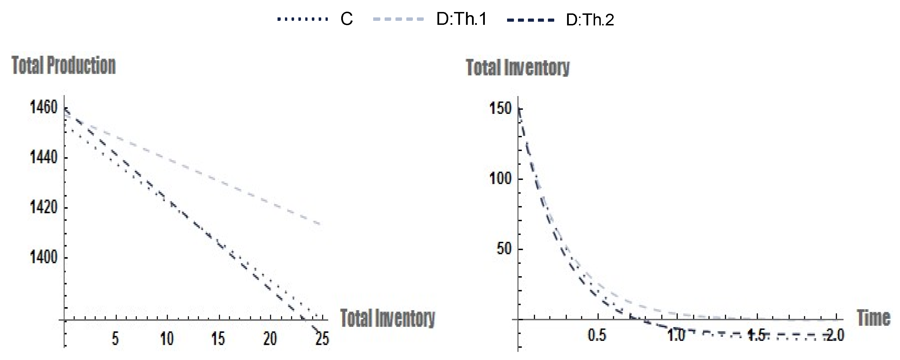
Consider the strategies under Theorems 2 and 3. (a) For lower values of inventory levels, the total production quantities of the Decentralized with Full Information strategy are higher than those under the Centralized strategy, (b) For higher values of inventory levels, the total production quantities under the Centralized strategy are higher than those under the Decentralized with Full Information strategy.
Proof.
See Appendix A.
Thus, Proposition 1 states the relationship between the total production quantities and the inventory level for the two strategies that result from Theorems 2 and 3. In addition, we also present the D strategy from Theorem 1. We illustrate the result in Figure 2, based on the parameters presented in (14). □
Proposition 2.
Consider the strategies under Theorems 2 and 3. (a) For earlier times, the total inventory (production) under the Decentralized with Full Information strategy is lower (higher) than under the Centralized strategy. (b) For later times, the total inventory (production) under the Decentralized with Full Information strategy is higher than under the Centralized strategy.
Proof.
See Appendix A.
Proposition 2 implies that in the long run, the Decentralized with Full Information strategy converges to a higher inventory (production) level than the Centralized strategy. In Figure 2 we present the behavior of the total production and inventory that results from Theorems 1–3, using the parameters for the base case presented in (14). □
In Figure 3, we present the behavior of the total profits emission costs as a function of time of strategies that result from Theorems 1–3, using the parameters for the base case presented in (14).
5. Sensitivity Analysis
In this section, we explore how the results obtained in this study change when uncertainty is introduced into the parameters. We explore the sensitivity of the objective function to uncertainty in the emission parameter, the inventory parameter, and the discount rate. We are interested in the percentage of change relative to the objective function at baseline. Each change in a parameter was made using changes ±90% with steps of 10% from the baseline value. In each case, the axis grid represents the deviation in percentage from the baseline value. We start with the inventory and emission parameters and then explore the discounting.
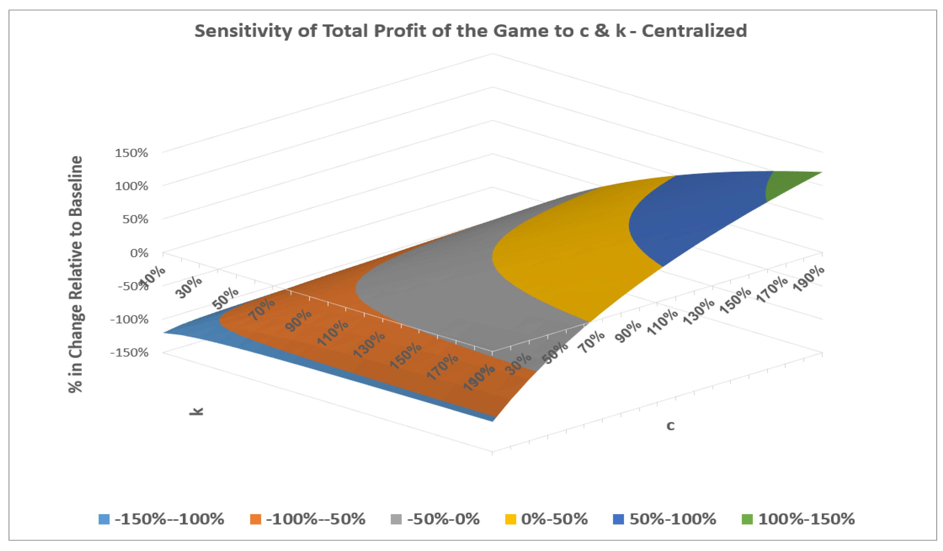
Sensitivity of Optimal Profits to c and k: In this case we do a two-dimensional sensitivity analysis, we obtain a surface since we have a tuple {parameter 1, parameter 2, objective value}. Consider Figure 4, which shows the results for the Centralized case. The figure indicates that the optimal profit in the Centralized setting is more sensitive to the inventory parameter than to the emission parameter, at least for larger values of the emission parameter. While the profit is nonlinearly dependent on k (for large values of c), it is linearly dependent on c (for almost all values of k). The graph for the Decentralized setting looks the same (and have the same scale). This is plausible since the various settings differ solely by a factor of k/c under the root.
Sensitivity of Optimal Profits to r: Discounting in such a setting is an impactful factor. We explored the discounting impact on profits in all three settings. The results showed that the optimal profits are linearly sensitive to changes in the range of [−20%, +20%]. However, in the range of +20% and more, the objective becomes flat, but in the range of −20% or less, it becomes very sensitive.
6. Conclusions, Managerial Implications, and Future Directions
In this paper, we analyzed a Decentralized with Full Information strategy of production decisions in a differential game framework involving profit maximizing output in an industrial park when emission costs are considered. The resulting dynamic game analyzed coordination through emission costs. Two alternative decentralized and centralized formulations were compared. In the case where decentralized firms can fully share information, the resulting equilibrium results in the best outcomes.
In our analysis we developed the optimal equilibrium production quantities and the resulting optimal trajectories of the inventory policies. The optimal policies show that inventories decrease over time and converge to a certain value, whereas the production quantities increase over time and converge to the total sales rate (except the fully coordinated case, which is proportional to the sales rates). Different patterns were observed. If the initial inventory is zero, the profit function has a global maximum and then decreases and converges to a certain value. If the initial inventory is greater than zero, the structure becomes more complex, but the final values converge to the same values as before. A centralized strategy yields lower profits than a decentralized with full information strategy. However, in the short term, the centralized approach results in lower total emission costs and higher total profits. We explored the sensitivity of total profits in each of the settings to key parameters.
The theoretical results derived in this paper on the coordination of emission considerations have crucial implications for management. There is no doubt that decentralization works if the units involved are appropriately coordinated. If they are not, pursuing divisional objectives results in severe profit losses. Hence, if a company wants to exploit the benefits of decentralization, it needs to implement a sound coordination policy, in which besides considering the production costs, they must consider the cost of emissions and coordinate these two forces. Management needs to weigh the benefits and losses arising from decentralization and choose a strategy that comes close to its best profit levels, while mitigating emissions in a balanced way.
Future research in this area could concentrate on several issues:
Uncertainty: adding uncertainty to the input of the problem could lead to greater insights and add more practicality to the model. More specifically, studies could explore the case where the cost parameters vary in a closed interval.
Stochasticity: If the knowledge base on the uncertain parameter is denser and frequencies can be derived, probability theory can be implemented to possibly determine the stochastic structure of these inputs, in which case a stochastic differential game should be pursued.
Setup cost: We assumed that changing the output rate would have no cost or time implications. In practice, any change in production capacity entails costs, such as changing the personnel supporting production or calibrating the manufacturing machines. Thus, it would be of interest to model such an extension and explore its impacts. We conjecture that this might affect the structure of the optimal policy.
Multiple Manufacturers: In an industrial park, there tend to be multiple manufacturers. It would be interesting to see how the structure of the optimal policy changes when there are multiple manufacturers and assuming different levels of coordination, e.g., coordination among individuals or groups of individuals.
Author Contributions
Conceptualization, G.E.F. and H.N.; methodology, G.E.F. and H.N.; software, G.E.F. and H.N.; validation, G.E.F. and H.N.; formal analysis, G.E.F. and H.N.; investigation, G.E.F. and H.N.; resources, G.E.F. and H.N.; data curation, G.E.F. and H.N.; writing—original draft preparation, G.E.F. and H.N.; writing—review and editing, G.E.F. and H.N.; visualization, G.E.F. and H.N.; supervision, G.E.F. and H.N.; project administration, G.E.F. and H.N.; funding acquisition, Not Relevant. All authors have read and agreed to the published version of the manuscript.
Funding
This research received no external funding.
Institutional Review Board Statement
Not Applicable.
Informed Consent Statement
Not Applicable.
Data Availability Statement
Not Applicable.
Acknowledgments
The authors acknowledge Felix Pepier and Benzion Shklyar for very helpful discussions.
Conflicts of Interest
The authors declare no conflict of interest.
Appendix A
To prove Theorems 1–3 we use techniques from [32].
Proof of Theorem 1.
To find the feedback strategies each player has the value function:
where , refer to the derivative of Vj with respect to Ij and Ii, respectively. The maximization with respect to qj yields
Or
Thus substituting (A3) into (A1) leads to (removing the arguments)
Note that in (A4) both appear. Solving the system of differential equations represented by (A4) means finding the value functions that satisfy them. The following value functions are proposed as solutions,
which implies, for
In order for the value functions proposed in (A5) to be solutions to (A4), the coefficients must have the “right” values. To find them, substitute last two equations into (A4) to get
This implies,
By manipulating (A8)–(A12) we obtain the coefficients of
Which completes the proof. □
Proof of Theorem 2.
To solve this problem we use the Hamiltonian approach. The Hamiltonian of this problem is
The maximization condition is
We denote , and , thus
Assume . Substituting into and we obtain
By comparing coefficients we obtain
Therefore,
And this completes the proof. □
Proof of Theorem 3.
The Hamiltonian of this problem is:
Let
And this completes the proof. □
Proof of Corollary 1.
By definition
Also
From (A14) and (A15) it follows that
Hence
Considering (A13)
Therefore,
Thus
Or
□
Proof of Proposition 1.
By definition
From (A16)
With respect to (A17), when, the total production rate, starts at a higher value in the Centralized setting than in the Decentralized with partial Information setting. However, as the total inventory increases and, given (A16), since the slope, in absolute values, of the Decentralized with Partial Information strategy is higher than that of the Centralized strategy, at some total inventory level the total production rate for the Decentralized with Partial Information strategy will be lower than that of the Centralized strategy. □
Proof of Proposition 2.
From (A13) can also be shown that
At t = 0 the total inventory, I1 + I2, starts at I0 and decreases with t. Given (A18), and (10), (13) the Decentralized with Partial Information strategy is higher than the Centralized strategy. However, as t increases, in long run the total inventory of the Decentralized with Partial Information is higher than the Centralized strategy. The part for production follows from this proof and from Proposition 1. □
References
- International Energy Outlook. World Energy Balance. 2020. Available online: https://www.iea.org/subscribe-to-data-services/world-energy-balances-and-statistics (accessed on 2 February 2021).
- U.S. Energy Information Administration (EIA). International Energy Outlook. 2019. Available online: https://www.eia.gov/outlooks/ieo/ (accessed on 2 February 2021).
- Poore, J.; Nemecek, T. Reducing Food’s Environmental Impacts Through Producers and Consumers. Science 2018, 360, 987–992. [Google Scholar] [CrossRef] [PubMed] [Green Version]
- Geng, Y.; Hengxin, Z. Industrial Park Management in the Chinese Environment. J. Clean. Prod. 2009, 17, 1289–1294. [Google Scholar] [CrossRef]
- Saikku, L. Eco-Industrial Parks—A Background Report for the Eco-Industrial Park Project at Rantasalmi; Publications of Regional Council of Etelaü-Savo: Tampere, Finland, 2007; p. 71. [Google Scholar]
- Vachon, S.; Mao, Z. Linking Supply Chain Strength to Sustainable Development: A Country-Level Analysis. J. Clean. Prod. 2008, 16, 1552–1560. [Google Scholar] [CrossRef]
- International Energy Outlook 2017. p. 10. Available online: https://www.eia.gov/outlooks/aeo/ (accessed on 2 February 2021).
- Katiraei, F.; Iravani, R.; Hatziargyriou, N.; Dimeas, A. Microgrids Management: Controls and Operation Aspects of Microgrids. IEEE Power Energy Mag. 2008, 6, 54–65. [Google Scholar] [CrossRef]
- Kennedy, J.P.; Wells, C. Construction of a Microgrid for Industrial Parks. Working Paper. Available online: http://www.gridwiseac.org/pdfs/forum_papers09/kennedy.pdf (accessed on 2 February 2021).
- Siemens White Paper. Microgrids 2011. Available online: https://www.climateaction.org/images/uploads/documents/Microgrids_as_a_solution_to_integrate_renewable_generation_Siemens_White_Paper.pdf (accessed on 2 February 2021).
- Mikhaylidi, Y.; Naseraldin, H.; Yedidsion, L. Operations Scheduling Under Electricity Time-Varying Prices. Int. J. Prod. Res. 2015, 53, 7136–7157. [Google Scholar] [CrossRef]
- Oren, S.S.; Smith, S.A. Design and Management of Curtailable Electricity Service to Reduce Annual Peaks. Oper. Res. 1991, 40, 213–228. [Google Scholar] [CrossRef] [Green Version]
- Baldick, R.; Kolos, S.; Tompaidis, S. Interruptible Electricity Contracts from an Electricity Retailer’s Point of View: Valuation and Optimal Interruption. Oper. Res. 2006, 54, 627–642. [Google Scholar] [CrossRef] [Green Version]
- Mohsenian-Rad, A.-H.; Wong, V.W.S.; Jatskevich, J.; Schober, R. Optimal and Autonomous Incentive-Based Energy Consumption Scheduling Algorithm for Smart Grid. In Proceedings of the 2010 Innovative Smart Grid Technologies (ISGT), Gothenburg, Sweden, 19–21 January 2010; pp. 1–6. [Google Scholar] [CrossRef] [Green Version]
- Mohsenian-Rad, A.-H.; Wong, V.W.S.; Jatskevich, J.; Schober, R.; Leon-Garcia, A. Autonomous Demand-Side Management Based on Game-Theoretic Energy Consumption Scheduling for the Future Smart Grid. IEEE Trans. Smart Grid 2010, 1, 320–331. [Google Scholar] [CrossRef] [Green Version]
- Barker, S.; Mishra, A.; Irwin, D.; Shenoy, P.; Albrecht, J. SmartCap: Flattening peak electricity demand in smart homes. In Proceedings of the 2012 IEEE International Conference on Pervasive Computing and Communications, Lugano, Switzerland, 19–23 March 2012; pp. 67–75. [Google Scholar]
- Bettoni, A.; Anghinolfi, D.; Paolucci, M.; Tonelli, F. Energy-aware scheduling for improving manufacturing process sustainability: A mathematical model for flexible flow shops. CIRP Ann. 2012, 61, 459–462. [Google Scholar] [CrossRef]
- Papier, F. Managing Electricity Peak Loads in Make-To-Stock Manufacturing Lines. Prod. Oper. Manag. 2016, 25, 1709–1726. [Google Scholar] [CrossRef]
- Silver, E.A.; Pyke, D.F.; Thomas, D.J. Inventory and Production Management in Supply Chains, 4th ed.; CRC Press: Boca Raton, FL, USA, 2017. [Google Scholar]
- Nahmias, S. Production and Operation Analysis, 5th ed.; McGraw-Hill/Irwin Inc.: New York, NY, USA, 2005. [Google Scholar]
- Chao, X.; Chen, F.Y. An Optimal Production and Shutdown Strategy when a Supplier Offers an Incentive Program. Manuf. Ser. Oper. Manag. 2005, 7, 130–143. [Google Scholar] [CrossRef]
- Battini, D.; Persona, A.; Sgarbossa, F. A sustainable EOQ model: Theoretical formulation and applications. Int. J. Prod. Econ. 2014, 149, 145–153. [Google Scholar] [CrossRef]
- Bouchery, Y.Y.; Ghaffari, A.; Jemai, Z.; Dallery, Y. Including sustainability criteria into inventory models. Eur. J. Oper. Res. 2012, 222, 229–240. [Google Scholar] [CrossRef] [Green Version]
- Glock, C.H.; Jaber, M.Y.; Searcy, C. Sustainability strategies in an EPQ model with price- and quality-sensitive demand. Int. J. Logist. Manag. 2012, 23, 340–359. [Google Scholar] [CrossRef]
- Chen, X.; Benjaafar, S.; Elomri, A. The carbon-constrained EOQ. Oper. Res. Lett. 2013, 41, 172–179. [Google Scholar] [CrossRef]
- Zanoni, S.; Bettoni, L.; Glock, C.H. Energy implications in a two-stage production system with controllable production rates. Int. J. Prod. Econ. 2014, 149, 164–171. [Google Scholar] [CrossRef]
- Elyasi, M.; Khoshalhan, F.; Khanmirzaee, M. Modified economic order quantity (EOQ) model for items with imperfect quality: Game-theoretical approaches. Int. J. Ind. Eng. Comput. 2014, 5, 211–222. [Google Scholar] [CrossRef]
- Dockner, E.; Fruchter, G.E. Coordinating Production and Marketing with Dynamic Transfer Prices. Prod. Oper. Manag. 2013, 23, 431–445. [Google Scholar] [CrossRef]
- Pekelman, D. Simultaneous Price-Production Decisions. Oper. Res. 1974, 22, 788–794. [Google Scholar] [CrossRef]
- Feichtinger, G.; Hartl, R.F. Optimal pricing and production in an inventory model. Eur. J. Oper. Res. 1985, 19, 45–56. [Google Scholar] [CrossRef]
- Erickson, G.M. A differential game model of the marketing-operations interface. Eur. J. Oper. Res. 2011, 211, 394–402. [Google Scholar] [CrossRef]
- Dockner, E.J.; Jorgensen, S.; Van Long, N.; Sorger, G. Differential Games in Economics and Management Science; Cambridge University Press (CUP): Cambridge, UK, 2000. [Google Scholar]
Figure 1.
A schematic depiction of the industrial park model.

Figure 2.
Total production quantities and total inventory.

Figure 3.
Total profits and emission costs as a function of time.
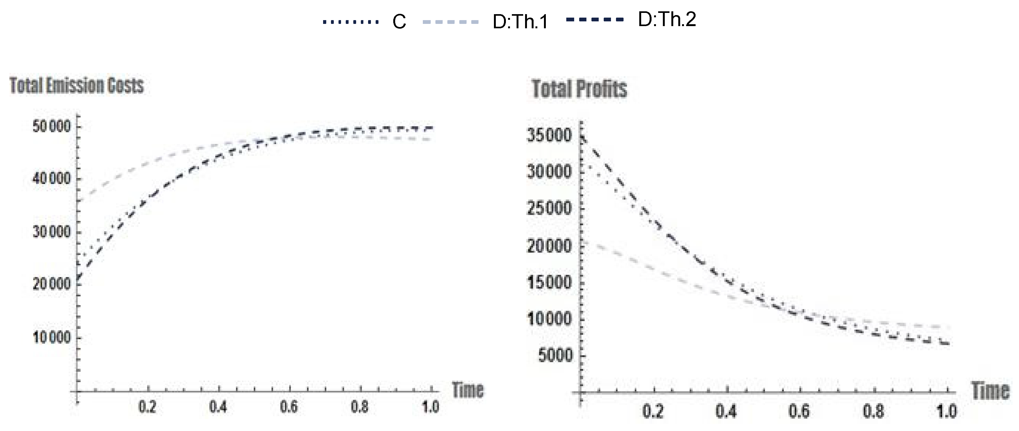
Figure 4.
Sensitivity of the Optimal Profit to c and k.

Publisher’s Note: MDPI stays neutral with regard to jurisdictional claims in published maps and institutional affiliations. |
© 2021 by the authors. Licensee MDPI, Basel, Switzerland. This article is an open access article distributed under the terms and conditions of the Creative Commons Attribution (CC BY) license (http://creativecommons.org/licenses/by/4.0/).
Share and Cite
MDPI and ACS Style
Fruchter, G.E.; Naseraldin, H. Coordinating Carbon Emissions via Production Quantities: A Differential Game Approach. Games 2021, 12, 15. https://0-doi-org.brum.beds.ac.uk/10.3390/g12010015
AMA Style
Fruchter GE, Naseraldin H. Coordinating Carbon Emissions via Production Quantities: A Differential Game Approach. Games. 2021; 12(1):15. https://0-doi-org.brum.beds.ac.uk/10.3390/g12010015
Chicago/Turabian StyleFruchter, Gila E., and Hussein Naseraldin. 2021. "Coordinating Carbon Emissions via Production Quantities: A Differential Game Approach" Games 12, no. 1: 15. https://0-doi-org.brum.beds.ac.uk/10.3390/g12010015
Note that from the first issue of 2016, this journal uses article numbers instead of page numbers. See further details here.