Fractional Punishment of Free Riders to Improve Cooperation in Optional Public Good Games


Polytechnic School, National University of Asuncion, San Lorenzo 2111, Paraguay
*
Author to whom correspondence should be addressed.
Games 2021, 12(1), 17; https://0-doi-org.brum.beds.ac.uk/10.3390/g12010017
Submission received: 7 September 2020
/
Revised: 11 January 2021
/
Accepted: 1 February 2021
/
Published: 5 February 2021
Abstract
:Improving and maintaining cooperation are fundamental issues for any project to be time-persistent, and sanctioning free riders may be the most applied method to achieve it. However, the application of sanctions differs from one group (project or institution) to another. We propose an optional, public good game model where a randomly selected set of the free riders is punished. To this end, we introduce a parameter that establishes the portion of free riders sanctioned with the purpose to control the population state evolution in the game. This parameter modifies the phase portrait of the system, and we show that, when the parameter surpasses a threshold, the full cooperation equilibrium point becomes a stable global attractor. Hence, we demonstrate that the fractional approach improves cooperation while reducing the sanctioning cost.
1. Introduction
Improving cooperation is a fundamental issue in human activities. The emergence and evolution of cooperation have been studied in life and social science; for instance, biologists have vastly studied altruism [1,2,3], and economists have studied social dilemmas [4,5]. In many cases, this problem has been modeled by using game theory [6,7] and, lately, with the development of evolutionary game theory [8] by using evolutionary dynamics models [9,10,11].
In the literature, two main mechanisms that affect cooperation are found: incentives and abstention. Incentives are known to improve the rate of cooperative behavior in a group [12,13,14,15,16,17], while abstention to participate in a project is useful to maintain cooperation [18,19]. However, incentives are expensive; for this reason, a punishment system is a public good itself [12].
In this paper, we consider improving cooperation by sanctioning only a fraction of the free riders, denominated from here onwards, as fractional punishment. This approach seeks to reduce the number of free riders while minimizing the cost of the sanctioning system. The punishment is built as an extension of the optional public good game model presented in [18].
Therefore, the optional public good game that will be analyzed in this paper consists of a set of randomly selected individuals from the population who shares an institutional service. Each of the individuals decides among three strategies: refuse to play, decide to play and contribute to the common pool (pay for the service), and decide to play but do not contribute (use the service but do not pay for it). In the public good game, the benefit from the common pool is divided equally among all the players. In this work, a fraction of the free riders are randomly selected, and their payoff is reduced to zero.
Sanctioning System
In public good games, the two well-studied forms of sanctioning free riders are peer punishment and pool punishment [20]. In peer punishment, after the game, an individual that contributed (a cooperator) can decide to use part of its payoff to sanction all the free riders in the population. On the contrary, pool punishment is defined before the game; each cooperator must decide to contribute or not to a second pool that will be later on used to sanction the free riders.
A cooperator that is willing to sanction free riders plays a punisher strategy. A punisher has to contribute to the game and to the sanctioning system. A cooperator that decides not to sanction free riders becomes themselves a free rider for the sanctioning system (called second-order free riders). With peer punishment, the cost for a small number of punishers in a group with mostly defectors prevents the punishers from prospering; conversely, in a group without defectors, cooperators and punishers have the same payoff. Therefore, punishers tend to disappear, allowing defectors space to invade the population. With pool punishment, this cannot occur since the punishers must contribute ex ante to the game. Pool punishment, however, is a fixed cost that exists even when there are no defectors in the population [20,21].
Both sanctioning methods were studied and compared in theoretical models and experiments [13,20,22,23]. For instance, it was found that pool punishment can stabilize cooperation if second-order free riders are also punished [21,22]. In addition, the second-order free-riding problem was analyzed in [23,24,25].
Peer and pool punishment are rarely applied in their pure form in practical situations. More recently, some authors have explored different ways to penalize free riders often inspired in real-life situations. In [26], the sanction that a defector has to pay is a fixed amount. Avoiding second-order free riding by introducing an entrance fee was analyzed in [15]. A set of the cooperators was randomly selected to perform as punishers in [27], the cost of punishing was shared between cooperators in [28], and a ceiling payoff for defectors was introduced to promote cooperation in [29,30].
In this work, we assume that the sanctions have to be implemented with the fee collected periodically in a fee pool. This is observed as a common practice in institutions that provide a service. Within this framework, second-order free-riding does not occur since those who pay for the service implicitly are paying for the sanctioning system. However, this also implies that the profit that each player receives is reduced, given that a part of the collected resources must be used to penalize free riders.
The institution decides the fee-pool portion that will be used for each expense: providing the service and sanctioning free riders. The sanctioning system may not be a fixed cost; when free-riding decreases, the fee-pool amount required to sanction free riders will also decrease. Besides, the institution may limit sanctioning expenses by penalizing only a fraction of the free riders.
The aim of this paper consists in modeling mathematically a fractional punishment mechanism commonly applied in real situations to reduce expenses. We prove that fractional punishment improves cooperation and reduces the cost of punishing, and full cooperation can be achieved when the fraction of sanctioned defectors surpasses a minimum. Moreover, depending on the size of the punished fraction, the cooperation can be attained faster. This means that, by adjusting the parameter, the fractional punishment modifies the nature of the equilibrium points of the system and the phase portrait itself. With this analysis, decision-makers of the institutions can produce scenarios to foresee the effect of the fraction sanctioned in the improvement of the cooperation.
This article is organized as follows: in Section 2, the proposed model and dynamic, as well as the definition of the payoff, are presented. In Section 3, the system is analyzed, and the equilibrium points are characterized as a function of the punishment parameter denoted by d. The implications of the model, along with the penalization of a limited set of the free riders, are discussed in Section 4, while some concluding remarks are finally presented in Section 5.
2. Materials and Methods
Consider a large population where from time to time n randomly selected individuals are offered to play in a public good game (; ). Those who refuse to play are known in the game as loners (). The loners have a payoff that is constant and independent of the game. Those who decide to play the public good game will receive their payoff from the game (). In the game, each player must decide if either contributes or not with a positive amount c to the common pool. Individuals who contribute are cooperators (), and those who do not are defectors (). The total contribution to the common pool (obtained from cooperators) is then multiplied by a factor r; in a public good game, the amount in the common pool is distributed equally between all the players, regardless of whether they are cooperators or defectors. Instead, in this work, a randomly selected set of defectors will be sanctioned reducing their payoff to zero.
For modeling the population dynamics, in this paper and following [11], every individual in the population follows a strategy i (for ) from the three options available: cooperators x, defectors y, and loners z.
Let be the frequency of each of the corresponding available strategies of the population at a specific time t. To simplify the notation, we drop henceforth the time dependency t and simply write x, y, and z. The frequency distribution of the whole population at a specific time t is defined by the state , which belongs to the unit simplex given by
The interior of is defined as the set of points where all strategies are present (i.e., x > 0, y > 0, and z > 0) and the boundary of is defined as the set of points that are not interior points. The boundary of the simplex comprises vertices and borders. The vertices x, y, and z represent a homogeneous population of cooperators, defectors, and loners, respectively. In the borders, , , and , one strategy is absent.
Assuming a large enough population in which generations blend continuously into each other, each strategy evolves with a rate that expresses its evolutionary success following the replicator equation
with , , and as initial conditions in the simplex , with , where is the payoff of the ith strategy, and is the average payoff of the population.
It is important to remark that the simplex remains invariant under the flow of Equation (2) (see [11,31]); hence, if the state at , then , and it is endowed with the standard norm . Notice that, in Expression (2), an important behavior relies on the payoff of the ith strategy with respect to the average population payoff in the sense that, if , then the proportion of the i strategy increases, otherwise it decreases. Next, the payoff of each strategy is defined.
Considering a group of cooperators, defectors, and loners and assuming that each contribution is equal , the payoffs of each strategy in an optional public good game without punishment is defined by [18,32]:
where the parameters r, , and n are considered under the following assumptions:
Assumption 1.
The interest rate on the common pool r satisfies .
If , i.e., if all individuals cooperate, they are better off than if all defects. If , each individual is better off defecting than cooperating [18].
Assumption 2.
The payoff of the loner strategy σ satisfies .
This means that the revenue of a cooperator in a group of cooperators (profiting each) is better off than loners that receive , but loners are better off than a defector in a group of defectors, where the payoff is equal to 0 [18].
To compute the payoff of a player in a group, consider that this group composition depends on the frequencies of all strategies in the population. In the sample group of size n, where s is the number of those who will participate (cooperators and defectors), and is those who refuse (loners), if , the game cannot take place, and the payoff will be equal to a loner payoff regardless of the strategy of the player, and this happens with a probability . If , an individual that agrees to play has coplayers from the sample given by the probability [18]
Furthermore, the probability that j of these coplayers will be cooperators and the other defectors is [18]
In this work, we consider that only a fraction d () of the defectors will be punished, modifying the payoff presented in (3). In particular, we assume that this set of randomly selected defectors will have their corresponding payoff reduced to 0, while the remaining free riders will obtain the normal payoff. Therefore, a defector not knowing if they will be punished or not, in the presence of j cooperators, will have a payoff equal to
The expected payoff for a defector in a group of s players over all possible numbers of cooperators is
Taking into consideration that a defector can be alone or in a group and that both the number or participants (s) and cooperators in the group are random variables, the average payoff for a defector over all possible numbers of participants is given by
Observing that , then the expression for can be rewritten as [18]
For the sake of simplicity, we define an auxiliary function . The payoff then finally takes the following form:
A similar analysis can be performed to obtain the expected payoff of a cooperator in the population. To distinguish the contribution from one cooperator to the contribution of the other cooperators in the group, the payoff can be rewritten:
where (the remaining cooperators in the game) is defined as j.
Therefore, the expected payoff for a cooperator in a group of players over all possible numbers of cooperators is
If the cooperator is the only one that wants to play, that is, if , the payoff is . If , the payoff depends on the number or participants (s) in the group. Hence, the expected payoff for a cooperator is given by
Observing that , we obtain
Rearranging and using, as before, the auxiliary function a, we obtain
The difference in payoff between defector and cooperator strategies shows the relative benefit (or drawback) of defectors over cooperators, and it is essential to characterize the solution orbits. This difference is given by
3. Results
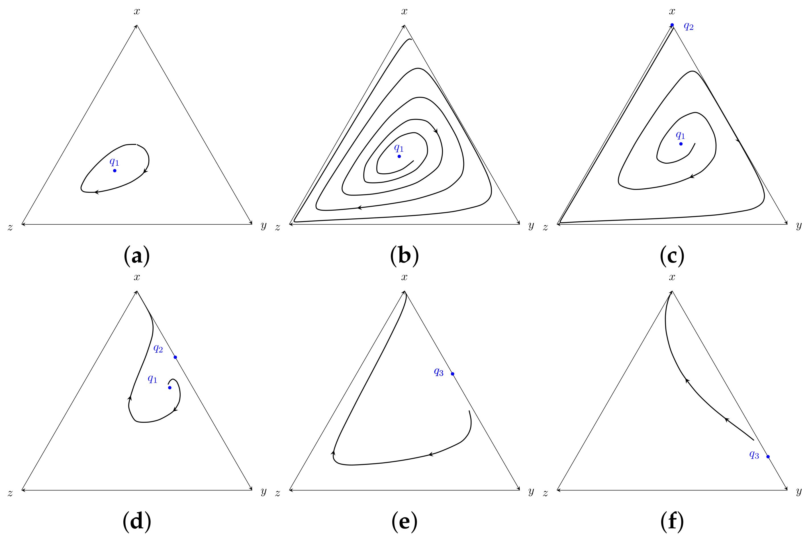
In this section, we analyze the system (2). To help the reader, and at the risk of oversimplification, before starting the analysis, we outline the effect of the parameter d on the phase portrait of the system (2). This is presented in Figure 1 for increasing values of d. Note that this system has three obvious equilibrium points, which are the vertices of the simplex: (i) (ii) , and (iii) . Another equilibrium point exists when all strategies have the same payoff , which is an interior equilibrium point (denoted as ). Later, we show that another equilibrium point arises when incrementing the value of d (this point is denoted by ).
For (no punishment), the vertices () are saddle points and the interior equilibrium () is a center (see Figure 1a), which is proved in [18]. The interesting effect of the punishment parameter d consists in the fact that the interior equilibrium point changes its stability (see Figure 1b). Furthermore, when d is large enough (), an interior equilibrium point arises () in the border (see Figure 1c). As a consequence, the nature of the equilibrium in the vertex x also changes. As d increases, the equilibrium point shifts to the border , and for a value , both equilibrium points ( and ) merge into a new equilibrium point denoted by (see Figure 1e). The nature of each of the aforementioned fixed points is studied in the next subsections.
For the analysis, we use the following sequence. In Section 3.1, the boundary of the simplex, particularly the border , where a new equilibrium point arises for a sufficiently large d, is analyzed. In Section 3.2, the interior of the simplex is analyzed. First, in Section 3.2.1 and Section 3.2.2, the effect of d in the position of the interior equilibrium point is considered, while in Section 3.2.3, the stability of the interior equilibrium point is analyzed. The stability of the equilibrium in the vertex x is analyzed in Section 3.3. A summary is presented in Section 3.4.
3.1. Boundary of the Simplex
In the borders, System (2) reduces to two equations. Next, we present the analysis of System (2) restricted to the boundary of .
3.1.1. Border
This border represents a system with cooperators and defectors, where the game is compulsory. Given that, in this border, , the dynamics can be analyzed with the following equation:
The equilibrium points are (), (), and . The qualitative characterization of the aforementioned equilibrium points were studied in [33] with the following lemma (see the proof in Appendix A.1).
Lemma 1.
Let us consider Equation (11) modeling the border where x denotes the cooperators, y the defectors, , , and . If the fraction of defectors being sanctioned is denoted by d, with and defining , then (1) for , the equilibrium point is locally asymptotically stable, (2) is locally asymptotically stable for , and (3) the point , which exists in the interior of the border for , is an unstable equilibrium point.
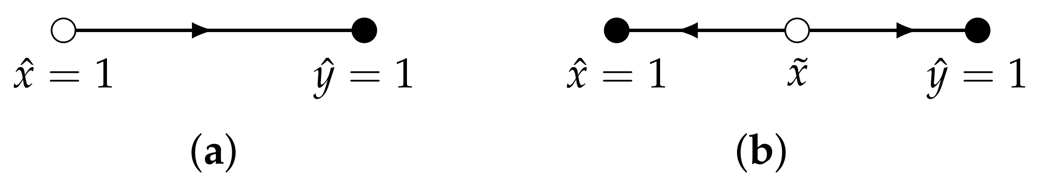
The possible outcomes of the system presented in Lemma 3.1 are sketched in Figure 2. It is important to mention the strong dependence of the characterization of the equilibrium points on the function . If 0 , then for all values of x, and the two equilibrium points are and . In such a case, the is globally unstable, and is globally asymptotically stable (see Figure 2a). For , an unstable equilibrium point arises in the interior of the border (see Figure 2b). If , then , the corresponding state x is the equilibrium point .
3.1.2. Border
This border represents a population of cooperators and loners. When , it is sufficient to analyze the equation to characterize the system. Since , the equilibrium points are () and (). When , the system remains constant, and every point in the border is an equilibrium point, regardless of the value of z. The Jacobian of has the following form:
Evaluating (12) shows that the equilibrium point () is stable (unstable) if . The dynamic of the border goes from only loners in the population to full cooperation. On the contrary, if , the equilibrium point () is unstable (stable) and the system reverses direction; it goes from full cooperation to a population of loners.
3.1.3. Border yz
This border represents a population composed of defectors and loners. Since , the system can be completely represented by . When , the equilibrium points are () and (). When , the system remains constant, and every point in the border is an equilibrium point, regardless of the value of z. The Jacobian of has the following form:
The equilibrium point () is unstable (stable) if . The dynamic in the border goes from full defection to a population of loners. Conversely, if , () is stable (unstable) and the system reverses direction, going from only loners to full defection.
Observe that the parameter d does not affect the borders and . Furthermore, since the game setup defines , the dynamic of the border goes from full defection to only loners in the population, while the dynamic of the border goes from only loners in the population to full cooperation.
3.2. Interior of the Simplex
To determine and analyze the interior equilibrium point, a new variable is defined [18]. This variable represents the fraction of cooperators among the players in the game and allows one to define a bijection , provided that the restriction is satisfied. Hence, the system (2) can be rewritten in a more convenient reduced form [18]:
where . The function is obtained replacing in Expression (10), so . To obtain a more explicit expression than (14), consider that , and . The system of Equation (14) can then be rewritten in the following form:
For each time t, d parametrizes the solution of the system of Equation (15). An equilibrium point of System (15) exists in the interior of the simplex if the following expressions are satisfied:
and since both equations have to be satisfied simultaneously, Equation (16b) is reduced to , so the value of f can be obtained by
By then introducing f in (16a), an equivalent definition for that depends only on z and d is obtained:
where and (as introduced in Expression (10)). Now, from (18), the value of z in the equilibrium, defined as , can be numerically obtained as a function of d. Recalling that a depends only on z (as defined in Section 2) and denoting as the expression of a with , then (16a) and (16b) become
where corresponds to the value of f at the equilibrium point associated with for a d. Defining an auxiliary variable as , the above equations take the form of a system of two equations with two unknowns ( and ), as follows:
Extracting from the second equation and introducing it in the first equation, is obtained. Replacing in the second equation, a new form of in the equilibrium is then obtained:
Notice that the interior equilibrium point corresponds in the system to the equilibrium point in the interior of the simplex given by
where and the dependence on the parameter d is given explicitly. To relate both systems, a summary of the equilibrium points with respect to the variables and its corresponding are given in Table 1.
The first three equilibrium points in Table 1 are the equilibrium points corresponding to the vertex of , the fourth in the interior of the simplex , and the fifth in the border . In the next subsections, the effect of d in the equilibrium point will be analyzed. For that reason, will henceforth be redefined as (for ) to distinguish from the equilibrium when , which will henceforth be defined as .
Before further analysis, let us define another threshold for the parameter d that will be used in the following sections. Notice that Expression (18) when is reduced to , from which can be obtained.
3.2.1. Effect of d over the Value of z in the Equilibrium
Here, the effect of parameter d on functions , , and in itself is analyzed. To this end, consider that, for , there is a value of such that (see Expressions (10) and (18)). We claim that the punishment parameter d, when , displaces the value to another such that with . To corroborate this affirmation about the effect of d, we introduce the following two lemmas. In all cases, Assumptions 1 and 2 are fulfilled. The prime symbol denotes the derivative of the function with respect to its independent variable, for instance, . We are interested in the relationships between and and between and for a small and for a z in the neighborhood of where .
Lemma 2.
Consider associated to such that . Let such that , and , , , and are negative. Thus, a) and b) .
The effect of the parameter d on the solution of with respect to the solution of of the free system model is analyzed in the following lemma (see the proof in Appendix A.3).
Lemma 3.
Considering the values of and associated to and such that and ; hence, .
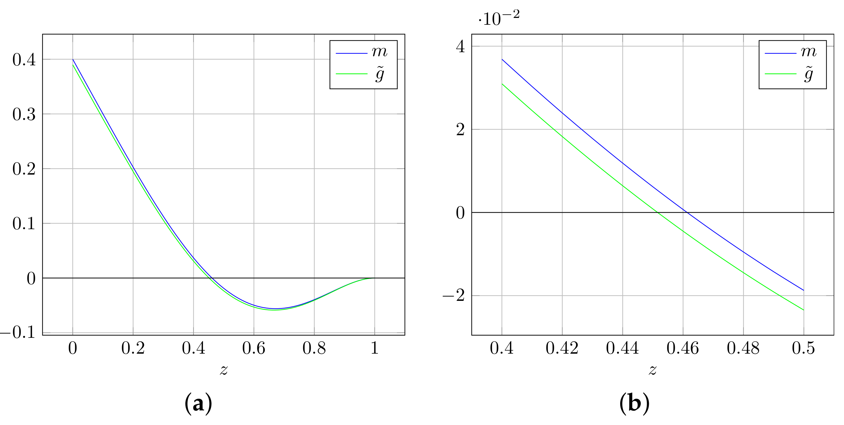
It is important to mention that, due to the value of d considered being small and the smoothness of and , the high order terms in the expansion in (A4) do not significantly affect the analysis and can be neglected. The results of Lemmas 2 and 3 can be observed in Figure 3, where the functions and for a with respect to z in the interval are presented. The effect of displacing to the left is observed; i.e., with is smaller than with .
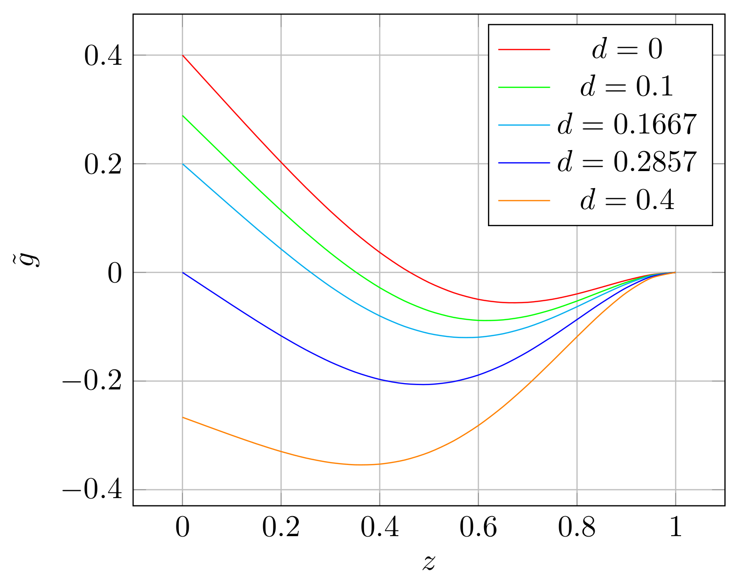
Figure 4 shows the evolution of with respect to several values of the parameter d (increasing values) remaining constant n, r, and . It can be observed that the main effect of the parameter d is precisely to displace to the left from its initial position. This property is exploited for the remainder of the article.
3.2.2. Effect of d over the Value of f in the Equilibrium
Here, the effect of the parameter d on the value of f in the equilibrium is analyzed. Recall that, at the interior equilibrium point, . Furthermore, due to game setup, (see [18]). As a consequence, we have the expression
for all . This means that, for a and its corresponding , , and , respectively, the following relationship holds:
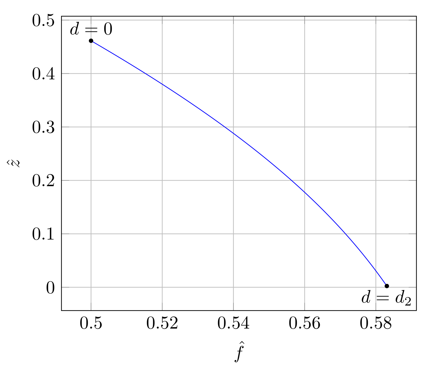
Therefore, the parameter d increments the equilibrium value or, equivalently, improves the level of cooperation. Figure 5 shows the changes in the value of and when d increases its value from 0 to . It can be seen how increases while decreases.
3.2.3. Effect of d in the Interior Equilibrium Point
Using the definition for a (introduced in (7)), Equation (14) (or equivalently Equation (15)) can be rewritten as follows:
For simplicity, we will drop the arguments in and write simply g. To characterize the equilibrium point at the interior of the simplex, we consider the Jacobian of System (24), which has the following form:
where
with , and .
In the interior equilibrium equilibrium point, and . Evaluating the Jacobian then yields
To simplify the analysis, considering the influence of the parameter d, we separate the Jacobian in two matrices and of dimension as with
and
It is important to mention that all the entries of the matrices and have bounded derivatives. If , the Jacobian matrix is reduced to . When (30) is evaluated at (), it becomes
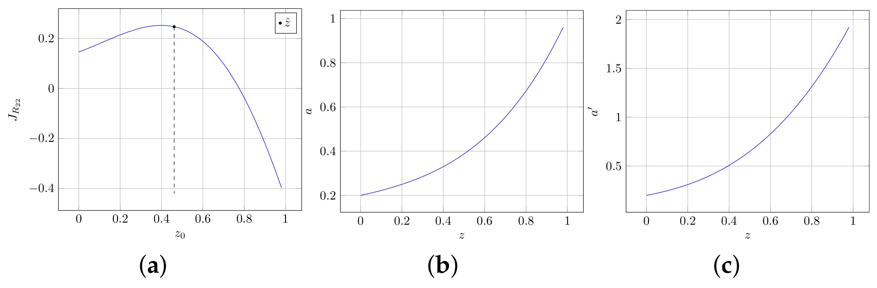
Since (see (21)), . The term is negative because . In addition, the term is positive, for and for the parameters n, , and r with values normally used in the literature. Figure 6a shows the value of for and particularly the value in the equilibrium ().
The eigenvalues of are given by , observing that is negative and is positive. The eigenvalues of are then pure imaginary. This result is important for the rest of the analysis of the interior equilibrium point when . The fact of the eigenvalues of J being pure imaginary is not conclusive when the interior equilibrium point is a center. However, we are assuming here that , so the system is reduced to the model in [18], which proves, using a Hamiltonian technique, that the interior equilibrium point is a center.
Next, we analyze the case of the Jacobian matrix J perturbed by the parameter d. To this end, we consider that . It is important to remark the implicit dependence of the matrices and on the parameter d.
Theorem 1.
Suppose a Jacobian matrix of System (24) denoted by J and decomposed as with entries and for with bounded derivatives. Suppose also an initial equilibrium point of System (24) that corresponds to the parameter , and another equilibrium point for denoted by . Thus, the Jacobian J, evaluated at with , has complex eigenvalues with positive real parts.
Theorem 1 (see the proof in Appendix A.4) shows that, for a small parameter d (considered positive), the eigenvalues of the Jacobian J of System (24) are complex with positive real parts when evaluated at the interior equilibrium point . This means that this equilibrium point is an unstable focus; i.e., all solution orbits of System (24) are repelled from the equilibrium point to the boundaries. This can be observed in Table 2, where some values of d, the corresponding equilibrium points , the entries of the Jacobian J, and its eigenvalues are shown. For , the eigenvalues of J are pure imaginary corresponding to the equilibrium point being a center. This result is consistent with the literature [18]. With small positive values of the parameter d ( and ), the eigenvalues have positive real parts, implying that the corresponding equilibrium point is an unstable focus in accordance with Theorem 1 (see also Figure 7a). It is important to mention that, for larger values of the parameter d ( ), the equilibrium point remains an unstable focus. Moreover, it is observed that is positive for and , as mentioned in Theorem 1.
As d increases, the equilibrium point changes its position from the equilibrium point with in the interior of the simplex towards the border by decreasing and increasing (see Section 3.2.1 and Section 3.2.2).
3.3. The Equilibrium Point
This equilibrium represents a homogeneous population composed exclusively of cooperators. When , this equilibrium point is a saddle point [19]. Now, we characterize this equilibrium point for and particularly for . For simplicity, the system (see (14)) will be used. As can be seen in Table 1, the equilibrium point corresponds to . Evaluating the Jacobian at this equilibrium point is obtained:
The eigenvalues of (33) are as follows: and . Notice that is negative given the condition in the game that (Assumption 2) and the choice of d determines the sign of . Recall that . Thus, for , is positive, and the equilibrium point is unstable (a saddle); however, if , is negative and the equilibrium point is locally asymptotically stable.
To better understand this equilibrium point and its basin of attraction, let us consider the relative-entropy function used in [10,34] as a candidate Lyapunov function.
Theorem 2.
Suppose that and the candidate Lyapunov function such that for all and for all . If
then , and the equilibrium point is locally asymptotically stable (see proof in Appendix A.5).
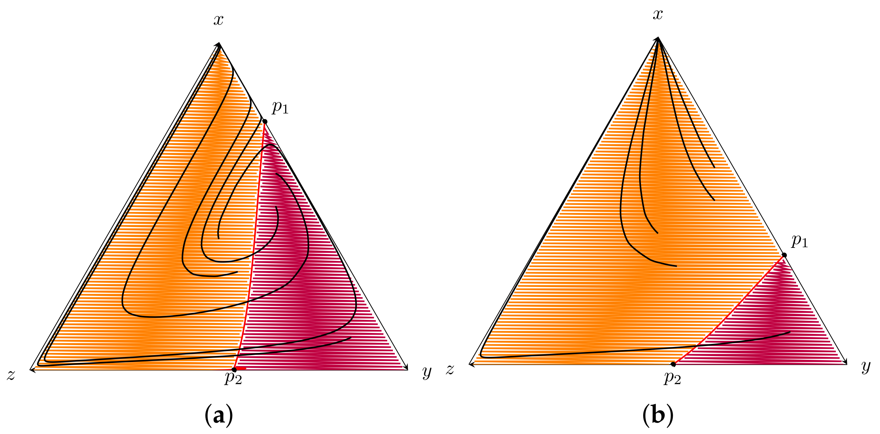
In Figure 8, the condition (34) is analyzed for increasing values of d, with the restriction , since this is a requisite for the equilibrium point to be stable. There are two main regions in the simplex. The region colored in orange contains all the states where , while the region colored in purple contains all the states where . Both regions are separated by a red line that divides the simplex from a point in the border (where ) defined as to another in the border (where ) defined as (see Figure 8). This division corresponds to the set of points where changes sign.
As d increases the region where also increases. This happens because the point moves to the vertex . Notice that the value of obtained from is . This is the position of the unstable equilibrium in the border analyzed in Section 3.1.1. The point , however, does not depend on d. When , the expression is reduced to (see (10)). Therefore, the value of z in the point is fixed and corresponds to the value of when as in [18].
Additionally, in Figure 8, some paths with initial value points from both regions— and —are shown. Due to the structure of the solution, even trajectories with initial values outside the basin of attraction are drawn inside and eventually end in the equilibrium point. In such a case, the equilibrium point is globally asymptotically stable.
Notice in Figure 8a that some trajectories oscillate before reaching the equilibrium. This is caused by the unstable equilibrium point in the interior of the simplex analyzed in Section 3.2. Recall that the interior equilibrium shifts to the border as d increases, reaching it when , which, for the parameter in Figure 8, is .
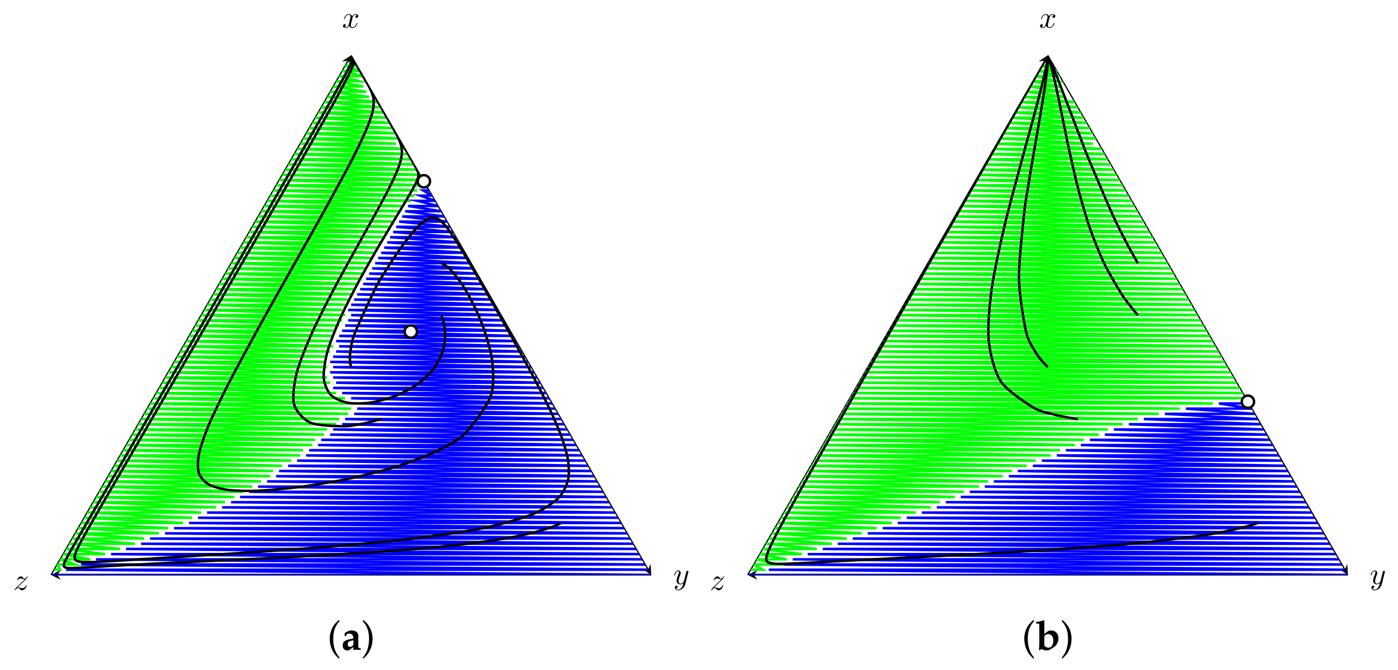
From a practical point of view, we are interested in trajectories where the frequency of cooperators does not decrease and, as a consequence, in the set of initial values from which the number of cooperators increases along all the trajectory to the equilibrium point. To observe this behavior, two regions are defined in the simplex ; we denote by a set of initial values where the frequency of the cooperator strategy in the solution orbits continuously grows until full cooperation is reached, i.e.,
In Figure 9, the region is in green. It can also be observed (and this is an important consideration) that is enlarged as the parameter d increases. In addition, the set of initial values in the simplex , where the frequency of cooperators decreases before reaching the equilibrium point, i.e., , is colored in blue.
3.4. Summary of the Fractional Punishment Effect in the System
In this section, we complete the outline presented in Figure 1 in Section 3. Notice that the whole effect of the parameter d in the dynamic and the equilibrium points of System (2) can be described using the thresholds and as introduced in Section 3.1.1 (Lemma 1) and Section 3.2, respectively.
Recall that, when , the interior equilibrium point is a center, and the vertices are saddle points [18]. Figure 1a shows the periodic orbits around the equilibrium.
Positive values of d cause two transformations in the system. First, the equilibrium point becomes unstable; second, the position of the equilibrium changes. It moves towards the border . Figure 1b shows how, with small values of d, , the trajectories approaching the border of the simplex oscillate.
As d increases, i.e., , a new equilibrium point arises in the border . This is an unstable equilibrium point that moves to the vertex y as d increments its value. Furthermore, when appears, the vertex x changes its nature from unstable (saddle point) to stable (see Figure 1c,d). Notice that the number of oscillations needed to reach the vertex x decreases as d grows.
When , the equilibrium point reaches the border and merges with the equilibrium point in the border. This new equilibrium remains unstable (see Figure 1e).
From to , there is no equilibrium in the interior of the simplex. The point continues to move toward the vertex y, but it does not reach the vertex; when , the equilibrium point on the border takes the value .
4. Discussion
In this work, we present a mathematical model in which a fractional punishment is incorporated in an optional public good game under the replicator dynamic. To design the model, we consider two common situations regarding the administration of institutions: (1) not all those who did not pay their fees can be punished due to a lack of resources; (2) both the service provided and the cost of the sanctioning system come from the fee paid by the users (fee pool).
Our proposal seeks to handle this situation by limiting the sanction to a random set of defectors, warranting at the same time both the economic feasibility and effective punishment to at least a reduced number of free riders.
To this end, we assume in the game that a randomly selected portion of free riders would be penalized, but we do not include a separate pool to be used to sanction defectors. With these assumptions, we eliminate the possibility of second-order free-riding and the cost of second-order punishment, since cooperators, when paying the fee, are also unintentionally contributing to penalizing free riders. Furthermore, the cost of the sanctioning system is mainly dependent on the size of the portion punished, and it may be adapted in accordance with the resources available to the institution.
Small values of d produce solutions that oscillate approaching the border. The effect of the parameter d on the trajectory towards the equilibrium point is an important issue. A wide excursion could jeopardize the survival of any institution because of the increment of the loners and the possibility that this triggers the disappearance of the active population.
As d increases, the participation in the game is improved by reducing the share of loners within the population. This can be understood by the convergence of the equilibrium point to the axis. For an appropriate minimum value of d, a population composed exclusively of cooperators can be achieved. If d surpasses a first threshold value , a new unstable equilibrium point arises in the border while the equilibrium point in the vertex x becomes stable. Then, when d achieves a second threshold value , the interior equilibrium point reaches the border, and both equilibria merge. Notice that, with fractional punishment, the equilibrium reaches the border with , whereas in the model introduced in [18], it occurs when .
Even with a value of d adequate to achieve full cooperation, the trajectories can oscillate depending on the initial composition of the population. In this context, the set of initial values from which full cooperation is attained through trajectories with an ever-increasing frequency of cooperators is of special interest. This set of points (denoted by in the results) increases as d increases.
The fractional punishment is a useful mechanism when resources are scarce; it can improve cooperation at a lower cost. However, with this approach, the pressure on the correct use of the contribution (fee pool) is higher, reaching a balance between the expenditure dedicated to the operation with the expenditure on sanction free-riding is more important. Sanctioning free riders improves cooperation but decreases the profit from the game. We consider that an adequate balance between both expenses is perhaps one of the characteristics of a successful institution.
5. Conclusions
We have analyzed the effect of randomly punishing a percentage of defectors in an optional public good game modeled using replicator dynamics. To this end, the payoff of the strategies is redefined to introduce a punishment parameter. This parametrizes the simplex phase diagram, modifying the trajectories of the strategies in the population as well as the nature of some important equilibrium points. A description of the main characteristics variations of the trajectories in the simplex due to the punishment parameter parametrization was presented, and for the equilibrium point that represents full cooperation, the basin of attraction was described. Future works include modeling how the institution decides to set the value of the parameter d (probably adaptive) and its optimal choice, as well as the redistribution to cooperators of the benefits taken from the punished free riders.
Author Contributions
Conceptualization, R.B., C.E.S. and G.B.; methodology, R.B., C.E.S.; formal analysis, R.B., C.E.S. and G.B.; writing—original draft preparation, R.B., C.E.S. and G.B.; writing—review and editing, R.B., C.E.S. and G.B. All authors have read and agreed to the published version of the manuscript.
Funding
This research was partially supported by FEEI-CONACYT-Prociencia Pos-007 and 14-INV-344.
Acknowledgments
Authors acknowledge the support given by FEEI-CONACYT-Prociencia Pos-007 and 14-INV-344. Authors acknowledge the PRONII. R.B acknowledges CONACYT for the scholarship.
Conflicts of Interest
The authors declare no conflict of interest.
Appendix A
Appendix A.1. Proof of the Lemma 1
Proof.
The Jacobian of the Equation (11), defined by has the following form:
When Expression (A1) is evaluated at equilibrium point , it takes the form . As a consequence, since , the eigenvalue is negative, and the equilibrium point is locally asymptotically stable. This also means that the reciprocal equilibrium point is locally asymptotically stable, since .
If Expression (A1) is evaluated at equilibrium point , the Jacobian depends on the value of the parameter d, i.e., . The eigenvalue is negative for , and is consequently locally asymptotically stable; however, if , then the eigenvalue is positive and is locally unstable.
In order to analyze the equilibrium point , it should be noticed that d and x are bounded between 0 and 1. If , then , which is the minimum value of x for which the equilibrium point exists. Notice also that the maximum value of x is 1, so , which is , the minimum value of d for which the equilibrium point exists. For , Expression (A1) takes the following form:
Given that and considering , the eigenvalue of (A2) is positive for positive values of d; therefore, for , the equilibrium point is unstable. □
Appendix A.2. Proof of the Lemma 2
Proof.
Part 1. Consider with and compare the expression (introduced in (18)) in two situations: (1) and and (2) and . Notice that is negative by the hypothesis. In addition, is negative since and d is positive. Hence, for and for .
Part 2. Consider with and . Thus,
Notice that is positive, and since and are negative, then . □
Appendix A.3. Proof of the Lemma 3
Proof.
Consider with . Thus, . Considering the Taylor series expansion truncated at the first order for as follows, i.e., high-order terms of the series are neglected, we have
Since and (because satisfies and ), .
Consider , performing a similar analysis for but now for . Thus,
and .
Using the results of Lemma 2, we obtain
Since and , it is possible to conclude that . □
Appendix A.4. Proof of the Theorem 1
Proof.
Consider
Thus, for a positive d and , we obtain
where the sign of is explicitly specified due to the structure of the entries of the matrix . It can be observed that , and are both negative (see Expression (31), and the values of a and in Figure 6b,c) and can be positive or negative depending on the value of f on the trajectory of the solution of System (24).
The eigenvalues of (A8) are obtained by
Rearranging the expression above, we can obtain the second-order equation in
with a solution
where the discriminant .
Analysis of . First observe that, from Expression (23), . By Assumptions 1 and 2, and recalling that , is positive. In addition, comparing and (see that in Expression (31)), and considering , then it is possible to observe that , which is controlled by . Hence, the term is positive.
Analysis of discriminant Δ. Observe that is an analytic function with respect to d (since it depends on ), and for . Considering the Taylor series expansion of with respect to the parameter d, is given by the expansion
where denotes the derivative with respect to the parameter d. Observe that d controls , since choosing arbitrarily d can make the term as small as is necessary.
In addition, the expression inside the discriminant takes the form
with all terms controlled arbitrarily by d. As a consequence, . In this case, the discriminant is
where the dominant term is ,since the remaining terms are arbitrarily small. Recalling that and have opposite signs and for a sufficiently small d, the discriminant is negative. As a consequence, the eigenvalues of (A8) are complex with a positive real part. □
Appendix A.5. Proof of the Theorem 2
For the proof of Theorem 2, and following [10], we consider the carrier of a given state as the set of pure strategies with the positive probability in that state. Similarly, we consider the domain of a given state as the set of states in the simplex where the pure strategies that are present in the carrier of the given state have positive probabilities.
Proof.
In the equilibrium point , only f has a positive probability; therefore, by using the concept of a carrier introduced above, the candidate Lyapunov function takes the following form:
with for all and for .
The derivative with respect of time of this candidate Lyapunov function is given by
Substituting given by Expression (15) in Expression (A13), we obtain
where in the equilibrium point and is negative when . To obtain a condition for the parameter d, the explicit form of (see Equation (14) ) is replaced in Equation (A14). Thus,
Observe that is negative if , or, equivalently,
References
- Hamilton, W.D. The genetic theory of social behavior. I and II. J. Theor. Biol. 1964, 7, 1–52. [Google Scholar] [CrossRef]
- Haldane, J.B. Population genetics. New Biol. 1955, 18, 34–51. [Google Scholar]
- Nowak, M.A. Five Rules for the Evolution of Cooperation. Science 2006, 314, 1560–1563. [Google Scholar] [CrossRef] [PubMed] [Green Version]
- Hardin, G. The Tragedy of the Commons. Science 1968, 162, 1243–1248. [Google Scholar]
- Ostrom, E. Governing the Commons: The Evolution of Institutions for Collective Action; Cambridge University Press: Cambridge, UK, 1990. [Google Scholar]
- Trivers, R.L. The Evolution of Reciprocal Altruism Published by: The University of Chicago Press Stable URL. Q. Rev. Biol. 1971, 46, 35–57. [Google Scholar] [CrossRef]
- Axelrod, R.; Hamilton, W. The evolution of cooperation. Science 1981, 211, 1390–1396. [Google Scholar] [CrossRef]
- Smith, J.M. Evolutionary game theory. Phys. D Nonlinear Phenom. 1986, 22, 43–49. [Google Scholar] [CrossRef]
- Taylor, P.D.; Jonker, L.B. Evolutionary stable strategies and game dynamics. Math. Biosci. 1978, 40, 145–156. [Google Scholar] [CrossRef]
- Weibull, J. Evolutionary Game Theory; MIT Press: Cambridge, MA, USA, 1997. [Google Scholar]
- Hofbauer, J.; Sigmund, K. Evolutionary Games and Population Dynamics; Cambridge University Press: Cambridge, UK, 1998; p. 323. [Google Scholar] [CrossRef] [Green Version]
- Yamagishi, T. The provision of a sanctioning system as a public good. J. Personal. Soc. Psychol. 1986, 51, 110–116. [Google Scholar] [CrossRef]
- Fehr, E.; Gächter, S. Altruistic punishment in humans. Nature 2002, 415, 137–140. [Google Scholar] [CrossRef] [PubMed]
- Sigmund, K. Punish or perish? Retaliation and collaboration among humans. Trends Ecol. Evol. 2007, 22, 593–600. [Google Scholar] [CrossRef] [PubMed] [Green Version]
- Sasaki, T.; Brännström, A.; Dieckmann, U.; Sigmund, K. The take-it-or-leave-it option allows small penalties to overcome social dilemmas. Proc. Natl. Acad. Sci. USA 2012, 109, 1165–1169. [Google Scholar] [CrossRef] [PubMed] [Green Version]
- Hauert, C.; Traulsen, A.; Brandt, H.; Nowak, M.A.; Sigmund, K. Public Goods With Punishment and Abstaining in Finite and Infinite Populations. Biol. Theory 2008, 3, 114–122. [Google Scholar] [CrossRef] [PubMed] [Green Version]
- Hilbe, C.; Sigmund, K. Incentives and opportunism: From the carrot to the stick. Proc. Biol. Sci. R. Soc. 2010, 277, 2427–2433. [Google Scholar] [CrossRef] [PubMed] [Green Version]
- Hauert, C.; De Monte, S.; Hofbauer, J.; Sigmund, K. Replicator dynamics for optional public good games. J. Theor. Biol. 2002, 218, 187–194. [Google Scholar] [CrossRef] [PubMed] [Green Version]
- Hauert, C.; De Monte, S.; Hofbauer, J.; Sigmund, K. Volunteering as Red Queen mechanism for cooperation in public goods games. Science 2002, 296, 1129–1132. [Google Scholar] [CrossRef] [PubMed] [Green Version]
- Sigmund, K.; Hauert, C.; Traulsen, A.; Silva, H. Social Control and the Social Contract: The Emergence of Sanctioning Systems for Collective Action. Dyn. Games Appl. 2010, 1, 149–171. [Google Scholar] [CrossRef] [Green Version]
- Traulsen, A.; Rohl, T.; Milinski, M. An economic experiment reveals that humans prefer pool punishment to maintain the commons. Proc. R. Soc. B Biol. Sci. 2012, 279, 3716–3721. [Google Scholar] [CrossRef] [Green Version]
- Sigmund, K.; De Silva, H.; Traulsen, A.; Hauert, C. Social learning promotes institutions for governing the commons. Nature 2010, 466, 861–863. [Google Scholar] [CrossRef] [Green Version]
- Hilbe, C.; Traulsen, A.; Rohl, T.; Milinski, M. Democratic decisions establish stable authorities that overcome the paradox of second-order punishment. Proc. Natl. Acad. Sci. USA 2014, 111, 752–756. [Google Scholar] [CrossRef] [PubMed] [Green Version]
- Ozono, H.; Kamijo, Y.; Shimizu, K. Punishing second-order free riders before first-order free riders: The effect of pool punishment priority on cooperation. Sci. Rep. 2017, 7, 1–6. [Google Scholar] [CrossRef] [PubMed]
- Sasaki, T.; Unemi, T. Replicator dynamics in public goods games with reward funds. J. Theor. Biol. 2011, 287, 109–114. [Google Scholar] [CrossRef] [Green Version]
- Dercole, F.; De Carli, M.; Della Rossa, F.; Papadopoulos, A.V. Overpunishing is not necessary to fix cooperation in voluntary public goods games. J. Theor. Biol. 2013, 326, 70–81. [Google Scholar] [CrossRef]
- Chen, X.; Szolnoki, A.; Perc, M. Probabilistic sharing solves the problem of costly punishment. New J. Phys. 2014, 16. [Google Scholar] [CrossRef]
- Zhang, C.; Zhu, Y.; Chen, Z.; Zhang, J. Punishment in the form of shared cost promotes altruism in the cooperative dilemma games. J. Theor. Biol. 2017, 420, 128–134. [Google Scholar] [CrossRef] [PubMed]
- Zhang, J.; Zhu, Y.; Chen, Z.; Cao, M. Evolutionary Game Dynamics Driven by Setting a Ceiling in Payoffs of Defectors. In Proceedings of the 36th Chinese Control Conference, Dalian, China, 26–28 July 2017; pp. 11289–11295. [Google Scholar]
- Zhang, J.; Zhu, Y.; Li, Q.; Chen, Z. Promoting cooperation by setting a ceiling payoff for defectors under three-strategy public good games. Int. J. Syst. Sci. 2018, 49, 2267–2286. [Google Scholar] [CrossRef]
- Zeeman, E.C. Population dynamics from game theory. In Global Theory of Dynamical Systems, Lecture Notes in Mathematics; Springer: Berlin/ Heidelberg, Germany, 1980; Volume 819, pp. 471–497. [Google Scholar] [CrossRef]
- Sigmund, K.; Haiden, N.; Hauert, C. The dynamics of public goods. Discret. Contin. Dyn. Syst. Ser. B 2004, 4, 575–587. [Google Scholar] [CrossRef]
- Botta, R.; Schaerer, C.; Blanco, G. Cooperation and punishment in community managed water supply system. In Proceedings of the Conference of Computational Interdisciplinary Science CCIS-2019, Atlanta, GA, USA, 19–22 March 2019. [Google Scholar]
- Sandholm, W. Population Games and Evolutionary Dynamics; Economic Learning and Social Evolution; MIT Press: Cambridge, MA, USA, 2010. [Google Scholar]
Figure 1.
Phase diagram of the system when d increases. Parameters , , and . For these values, and . Notice that , , and are equilibrium points. (a) , (b) , (c) , (d) , (e) , and (f) .
Figure 1.
Phase diagram of the system when d increases. Parameters , , and . For these values, and . Notice that , , and are equilibrium points. (a) , (b) , (c) , (d) , (e) , and (f) .

Figure 2.
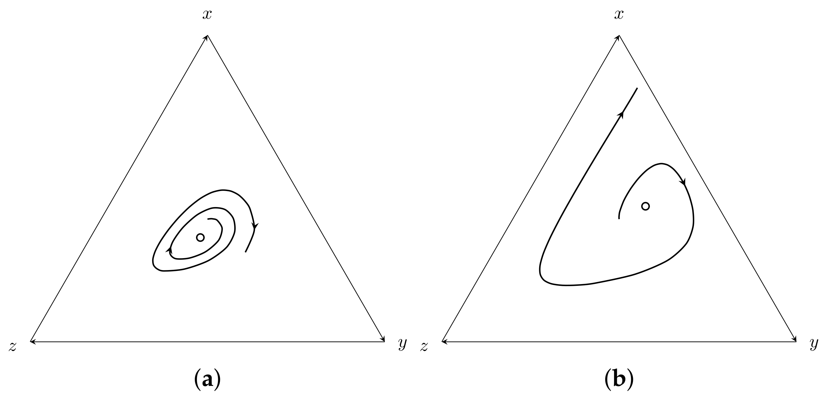
Stability of equilibrium points with different values of d: a black dot represents a stable point, and a white dot represents an unstable point. (a) With , the is unstable and is asymptotically stable. (b) If , an unstable equilibrium , denoted by , appears, changing the stability of , which becomes an stable equilibrium point.
Figure 2.
Stability of equilibrium points with different values of d: a black dot represents a stable point, and a white dot represents an unstable point. (a) With , the is unstable and is asymptotically stable. (b) If , an unstable equilibrium , denoted by , appears, changing the stability of , which becomes an stable equilibrium point.

Figure 3.
(a) and with . In the whole interval , (b) Zoom in the neighborhood of and . It can be observed that d decreases the value of in the equilibria. It shows how d shifts the equilibrium point to the border of . Parameters: , , and .
Figure 3.
(a) and with . In the whole interval , (b) Zoom in the neighborhood of and . It can be observed that d decreases the value of in the equilibria. It shows how d shifts the equilibrium point to the border of . Parameters: , , and .

Figure 4.
Graph of with several values of d. Observe that, if , when . Parameters: , , and .

Figure 5.
Interior equilibrium point and for increasing values of d. Observe that, when d increases, the value of increases, and the value of decreases. Parameters: , , , and .
Figure 5.
Interior equilibrium point and for increasing values of d. Observe that, when d increases, the value of increases, and the value of decreases. Parameters: , , , and .

Figure 6.
(a) Values of for and ; for , the term is positive. (b) Values of a for . (c) Values of for . Parameters: , , and .
Figure 6.
(a) Values of for and ; for , the term is positive. (b) Values of a for . (c) Values of for . Parameters: , , and .

Figure 7.
Effect of d on the interior equilibrium point. Parameters , , and , and values of d as (a) and (b) . The white dot represents an unstable point.
Figure 7.
Effect of d on the interior equilibrium point. Parameters , , and , and values of d as (a) and (b) . The white dot represents an unstable point.

Figure 8.
Values of for each possible state of the system. The orange area represent states ; the purple area represent states . The red line between both regions represent the set of points where changes sign. The black lines are trajectories from several initial values in the simplex. Parameters , , and , and increasing values of d: (a) and (b) .

Figure 9.
The behavior of x in the trajectories for each possible initial value. The green area represents initial values where the frequency of cooperators x increases along the orbit; the blue area represents initial values where at some point of the trajectories x decreases. The black lines are trajectories from several initial values in the simplex. , , and , and values of d are (a) and (b) .


Table 1.
Equilibrium points relationship between and . , .
Table 2.
Effect of the parameter d on the entries of the Jacobian J evaluated at equilibrium point and its corresponding eigenvalues. For , = . Parameters , , and ; and .
Table 2.
Effect of the parameter d on the entries of the Jacobian J evaluated at equilibrium point and its corresponding eigenvalues. For , = . Parameters , , and ; and .
| d | |||
|---|---|---|---|
Publisher’s Note: MDPI stays neutral with regard to jurisdictional claims in published maps and institutional affiliations. |
© 2021 by the authors. Licensee MDPI, Basel, Switzerland. This article is an open access article distributed under the terms and conditions of the Creative Commons Attribution (CC BY) license (http://creativecommons.org/licenses/by/4.0/).
Share and Cite
MDPI and ACS Style
Botta, R.; Blanco, G.; Schaerer, C.E. Fractional Punishment of Free Riders to Improve Cooperation in Optional Public Good Games. Games 2021, 12, 17. https://0-doi-org.brum.beds.ac.uk/10.3390/g12010017
AMA Style
Botta R, Blanco G, Schaerer CE. Fractional Punishment of Free Riders to Improve Cooperation in Optional Public Good Games. Games. 2021; 12(1):17. https://0-doi-org.brum.beds.ac.uk/10.3390/g12010017
Chicago/Turabian StyleBotta, Rocio, Gerardo Blanco, and Christian E. Schaerer. 2021. "Fractional Punishment of Free Riders to Improve Cooperation in Optional Public Good Games" Games 12, no. 1: 17. https://0-doi-org.brum.beds.ac.uk/10.3390/g12010017
Note that from the first issue of 2016, this journal uses article numbers instead of page numbers. See further details here.