Parties’ Preferences for Office and Policy Goals

Department of Political Science, The University of North Carolina at Chapel Hill (UNC), Chapel Hill, NC 27599-3265, USA
Games 2021, 12(1), 6; https://0-doi-org.brum.beds.ac.uk/10.3390/g12010006
Submission received: 30 October 2020
/
Revised: 18 December 2020
/
Accepted: 29 December 2020
/
Published: 14 January 2021
(This article belongs to the Special Issue Government and Coalition Formation)
Abstract
:Although parties’ preferences for office and policy goals have been featured by many rational choice models of party behavior and a majority of coalition theories, the literature still lacks a measure and a comprehensive analysis of how parties’ preferences vary among parties and across countries. This study aims to fill this gap by presenting the results of an original expert survey protocol, which finds that parties pursue both goals simultaneously as office is sought both as and an end and as a means to affect policy, and that the degree to which they prefer policy versus office objectives varies across parties and countries. I provide an application of the preference ratings for policy versus office in the context of government formation, by using the ratings to solve for and predict the equilibrium coalition that should have formed in Spain after the 2015 elections. The government predicted by the model matches the government that formed, providing evidence of the ability of the preference ratings to generate reliable predictions of the composition of government coalitions.
1. The Importance of Parties’ Preferences Regarding Policy and Office
Parties’ preferences for office and policy are the most important factor determining their behavior. The goals that political agents pursue are key to understanding and predicting how they behave, both in office and in opposition. Party goals determine the type of government that forms [1], the decisions to change or compromise on political programs [2,3], and the parties’ support for the political system [4]. Traditionally, political agents have been classified either as office seeking or policy pursuing, with the former aiming at achieving power [5] and the latter being more interested in the ultimate policy outcome [6]. However, parties’ preferences are more complex than the formal literature traditionally assumes: political agents are rarely motivated exclusively by just one of these goals, but they differ in the degrees to which they prefer one goal over the other [7].
Even though parties’ preferences have been a feature of most rational choice models of party behavior and an increasing number of empirical works, the literature still lacks a comprehensive analysis of how parties’ preferences vary among parties and across countries. This study aims to fill this gap by presenting the results of a survey of political experts from sixteen Western European countries, who were asked to evaluate parties’ positions and behavior on a variety of scales.
The survey design builds on the foundational expert survey study of Laver and Hunt [8], which constitutes the first contribution to the measurement of parties’ preferences regarding office and policy. However, the present survey departs from Laver and Hunt’s by introducing new dimensions on which the experts rate parties. These new dimensions differ substantially from Laver and Hunt’s assessments in that they allow office and policy goals to potentially be pursued together rather than assuming that these goals are incompatible. This assumption is consistent with the vast majority of the theoretical literature, which claims that policies can be changed mainly by the agents who control executive offices (see the literature from [9] to [10]).
The results of this study show that allowing for the compatibility of the two goals may yield significantly higher preference ratings for policy versus office. This can be crucial, especially in testing the predictions of government formation models, which are highly sensitive to parties’ preferences and require parties that are extremely motivated by policy in order to predict minority or surplus government coalitions that are frequently observed in Western European countries [11].
The paper presents an application of the preference ratings for policy versus office in the context of government formation. I present an analysis of the government formation process that took place in Spain in the aftermath of the 2015 elections. I solve for the equilibria generated by a simplified theoretical model of government formation using the preference ratings for policy versus office provided by the expert survey. The equilibrium government predicted by the model matches the government formed after the 2015 general election, providing evidence of the ability of the preference ratings to generate reliable predictions of the composition of government coalitions.
This paper proceeds as follows. The next section discusses the importance of parties’ preferences. Section 2 describes how parties’ preferences are conceptualized and measured. Section 3 describes the specifics of the survey. Section 4 presents the results and robustness checks to establish the soundness of the preferences’ measure. Section 5 presents an application of the parties’ preference measure in the context of government formation. Section 6 concludes.
Parties’ preferences regarding policy and office goals have been featured prominently in the government formation literature. Coalition formation theories can be divided in two main theoretical approaches: the “size and ideology” approach and the “new institutionalism” approach.
Theories belonging to the first approach relied on the tools of cooperative game theory and spatial modeling to analyze the formation of coalitions as function of parties’ size and ideology. Most of the early coalition formation literature assumed parties to be exclusively motivated by office benefits. Parties pursue their objective of maximizing their control over office by dividing the benefits of office with as small a number of partners as possible, leading invariably to the conclusion that only minimal-winning coalitions form [12]. In the 1970s, coalition theories started to postulate that office-motivated politicians were interested not only in maximizing their office benefits but also in minimizing the “transaction costs” of the bargaining process over the coalition policy, predicting the formation of coalition that are minimal winning in size but also ideologically connected.1 The intuition of this result is that policy agreements and compromises are more likely if the parties are ideologically close.
The “new institutionalism” tradition sprouted in the 1980s and focused on the role of institutions and the set of rules and norms governing the process of government formation as key variables of the coalition formation process [20,21,22,23]. They relied on the tools of non-cooperative game theory and, similarly to their predecessors, assumed parties that are both office seeking and policy-motivated. Some theories perceive these two objectives as substitutes, assuming that office poss can be traded off in exchange of “policy concessions” [24,25,26]. Some other theories [7,11] extend this idea by allowing for heterogeneity among parties’ policy and office preferences. The introduction of heterogeneity of policy goals allows these models both to explain why minority and surplus government coalitions form in equilibrium and to predict the composition of the government coalition as a function of parties’ preferences regarding the two goals.
Depending on the parties’ relative importance of “office” vis a vis “policy” motivations, coalition theories are able to predict equilibrium governments which can be minority, minimum winning, or surplus coalitions. Ideological divisions in the opposition is key for the viability of minority cabinets: the more ideologically divided opposition parties are, the greater the chances that a minority cabinet survives [1]. This is a major point of departure from the previous theoretical literature which had consistently predicted minimum winning (or minimum winning connected) coalitions in equilibrium.
Party goals have started to receive attention as determinants not just of coalition formation but also of party change. Party goals are perceived to be a key feature explaining why and how parties respond to changes in the electoral environment or political system. Parties that are more concerned about electoral prospects (office of vote-maximizing parties) are more likely to change their issue positions and organizational structure than parties that are more interested in policy goals [2]. The willingness of parties to change toward more moderate positions is also studied as a function of the parties’ preferences regarding office and policy and of their “ideological rigidity.” Parties with high ideological rigidity might be better off by staying out of office than by moderating their issue positions in order to get into office when the ideological sacrifice that moderation involves is too large [27]. Once in office, the larger the range of policies that a party can agree on, the less the party is motivated by policy goals [3]. Parties’ goals also affect parties’ support for the political system: office-pursuing parties are more likely to support the political system, while policy-pursuing parties are more willing to challenge the status quo and undertake institutional changes [4].
2. Conceptualizing and Measuring Parties’ Preferences for Policy Versus Policy Goals
Parties’ preferences regarding policy and office are difficult to measure, as they are usually inferred through the analysis of the parties’ past actions, such as the decision to coalesce with certain parties rather than others. When parties are exclusively office motivated, they are expected to form smaller coalitions (specifically the smallest winning coalition), while when they are purely policy pursing, they prefer to form coalitions with parties with similar ideal policies. However, focusing on coalition bargaining decisions excludes parties that have never taken part in government negotiations. Additionally, it abstracts away from other types of decisions that are signals of their preferences regarding office and policy, such as the intensity with which parties pursue legislation in certain areas of interest, the desire to control some ministries rather than others, and the willingness of parties to modify their electoral platform to attract more voters.
One way is to analyze the parties’ mission statement texts, parties’ manifestos, or other secondary sources in order to assess how the parties prioritize their goals, as in reference [30], who rank parties’ preferences regarding four main goals: votes, office, policy, and democracy. In this approach, potential behavior and actions of the parties that the researcher deems to be informative can be included and taken into account. Although ideal, this method requires the collection of parties’ materials and secondary sources that is not currently available for all parties or in all countries.
An alternative approach that allows researchers to take into consideration all of the parties’ signals is to rely on country experts’ assessments. Intuitively, the country expert serves as a “black box” in which all the signals are considered, weighted by importance and their ability to convey proxies of the parties’ preferences regarding office and goals, and aggregated by the expert. Although relying on subjective assessments might appear inferior to using observable data, the use of expert surveys for this task is instead ideal. Country experts are able to form beliefs about parties’ preferences based on their knowledge and observation of the parties’ history of actions and signals above and beyond what measurable data could provide. In fact, country experts are not only knowledgeable about the nuances of parties’ behavior, but they are also informed about the weight each parties’ actions should have in the overall assessment of their preferences.
Laver and Hunt’s expert survey [8], henceforth referred to as LH, is the first and only attempt to measure parties’ preferences for office versus policy in this way. In their survey, experts were asked, “Forced to make a choice, would party leaders give up policy objectives in order to get into government or would they sacrifice a place in government in order to maintain policy objectives?”.
The LH study constitutes a key contribution to the understanding of parties’ preferences. However, the framing of their question might induce respondents to assign scores that are more skewed toward office goals rather than policy goals. In fact, the question specifies two extreme events in which parties are willing to give up either policy or office objectives entirely, implicitly assuming that policy and office are to be considered as orthogonal goals. However, office and policy goals are not incompatible objectives. On the contrary, parties are able to affect policy mainly through the control of offices (i.e., cabinet portfolios), rendering the two factors dependent upon one another. This is true not only when a single party controls the executive office, but also in the case of government coalitions. Ministers have considerable power in the policy areas that fall under their jurisdiction, meaning that control over ministerial posts and policy-making power go hand in hand [9]. Government coalition parties in fact often obtain the executive offices that give them control of the policy areas about which they care the most [31]. Hence, political parties which are extremely policy motivated but also pragmatic might not be willing to give up office to maintain policy objectives. Rather, they might prefer to take office and be part of a government coalition which implement policies that are slightly more moderate than their ideal policies, but superior to the policies that an alternative government would implement.
To measure parties’ office and policy preferences while also allowing for their pragmatic desire to seek control over office for the pursuit of policy objectives, I conducted a new expert survey that asked the respondents to assess party preferences for policy versus office goals by means of a question that allows for the compatibility of the two goals. Specifically, the respondents were asked, “Suppose a party can form a government coalition with two alternative partners (or groups of partners). Would party leaders choose to form a coalition that gives their party the largest share of cabinet portfolios OR would they rather choose to form a coalition that would guarantee the implementation of a government policy closest to their ideal policy?”. Additionally, I asked respondents to assess the party’s position on several additional dimensions that could be expected to be affected by office and policy preferences to check for the robustness of the preference measure. In the next section, I describe the specifics of the survey.
3. An Expert Survey
The survey, which covers 16 Western European parliamentary democracies, was conducted between 29 October and 15 December 2015. In Table 1, I report the number of respondents per country. Because most surveys set five as a minimum standard number of respondents [8,32], the results of Luxembourg are excluded from the rest of the analysis. The appendix reports the survey methodology and the names, abbreviations, and logos of all parties included in the survey.
The respondents were asked to assess the parties’ position on several dimensions. The first dimension is the parties’ positions on the general left–right scale, L-R, ranging from −10 (extreme left) to 10 (extreme right). The second dimension, LH pol/off, measures the parties’ tradeoff between office and policy goals, assuming the two goals to be orthogonal. For this question, I used the same wording of the LH survey and a range from 0 (give up place in government) to 10 (give up policy objectives). The third dimension, New pol/off, captures parties’ preferences for policy versus office goals with a framing that allows for the compatibility of the two goals, as specified in the previous section, with a range from 0 (coalesce to maximize portfolio) to 10 (coalesce to maximize policy closeness). The last three survey questions serve to test some important theoretical assumptions. The fourth dimension, Portfolio, measures whether cabinet portfolios are valued more as an end (value equal to 0) or as means to affect policy (value equal to 10. The fifth dimension, Institutional change, assesses parties’ support for institutional changes, with a range from 0 (support political system) to 10 (propose institutional changes). The sixth dimension, Platform Change, evaluates parties’ willingness to change their policy positions and the direction of a possible change, with a range from −10 (taking more moderate policies), 0 (stay firm on ideological principles), and 10 (taking more extreme policies).2
3.1. Validity
The ideal check for content (or external) validity would be to cross-validate the assessments of this survey against other existing and independent measures widely accepted as valid [33,34,35]. Unfortunately, this cannot be done, as the only study that ever attempted to analyze parties’ preferences over office and policy goals [8] refers to a political environment of more than 25 years ago and does not represent an appropriate point of comparison. Not only have several parties dissolved or formed in the past 25 years, but parties have also undertaken new directions, experienced different histories, and lived through and with different political institutions. Furthermore, the present survey includes new dimensions and measures that have not previously been assessed in other studies. However, as Benoit and Laver argue, “As a check on content validity of our estimates, it is helpful to compare at least some aspects of our measures with measures generated by a well-known, widely used, published measurement instrument” ([36], page 95). The survey ratings for the parties’ positions on the general left–right dimension present an opportunity for direct comparison with other existing independent measures. To the extent that the two independent measures agree, we can be confident of the validity of this survey.
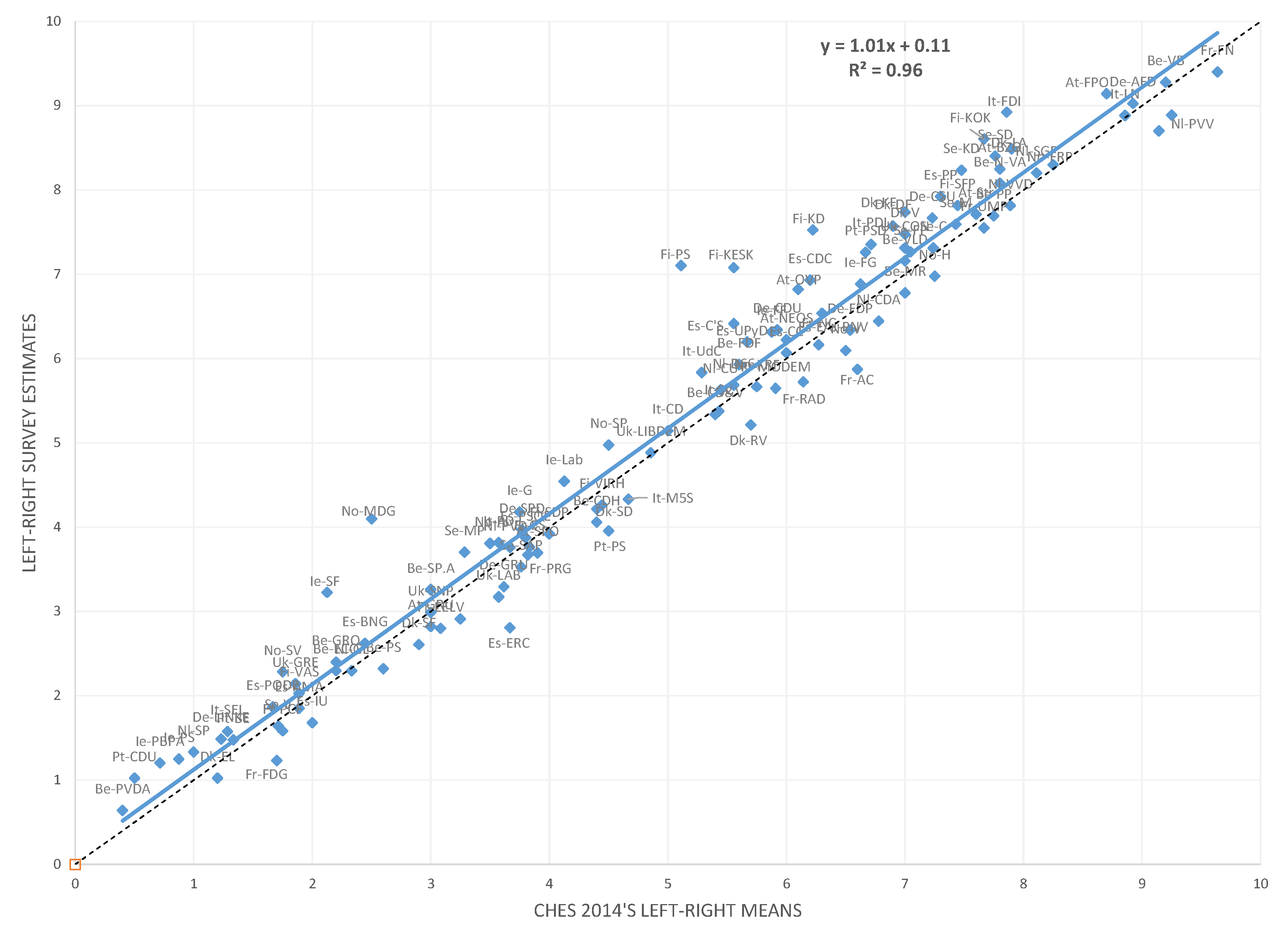
The most recent measure of parties’ left–right general position is used in the recent wave of expert surveys conducted by Chapel Hill Expert Survey (henceforth referred to as CHES) in 2014 [32]. Except in the case of a few parties that have become relevant since the time of those surveys and a few countries that have had general elections in 2015, CHES provides a perfect point of comparison in terms of the political environment of the countries under consideration. In Figure 1, I plot the survey’s mean estimates of the left–right general position (on the vertical axis) over the CHES’ mean estimates of the left–right general positions (on the horizontal axis) for all parties for which both estimates are available.
Each party is identified with a country and party code. The dotted 45-degree line represents the perfect match between the two surveys’ assessments. The solid line is the fitted linear regression line. The two lines overlaps almost perfectly, providing support for the cross-validation hypothesis. Furthermore, the linear relation provides an excellent fit between the two measures (with an of 0.96). There are a few outliers, mostly among the Finnish parties–the Centre Party of Finland (Fi-KESK), the Finns Party (Fi-PS), and the Christian Democrats (Fi-KD)–with a divergence between the two surveys’ ratings of more than one point on the 11-point scale (1.52, 1.99, and 1.30, respectively). The few remaining outliers include the Irish party Sinn Féin (Ie-SF), the Italian party Brothers of Italy (It-FDI), and the Norwegian Green Party (No-MDG), with a divergence of 1.10, 1.07, and 1.60 points, respectively.
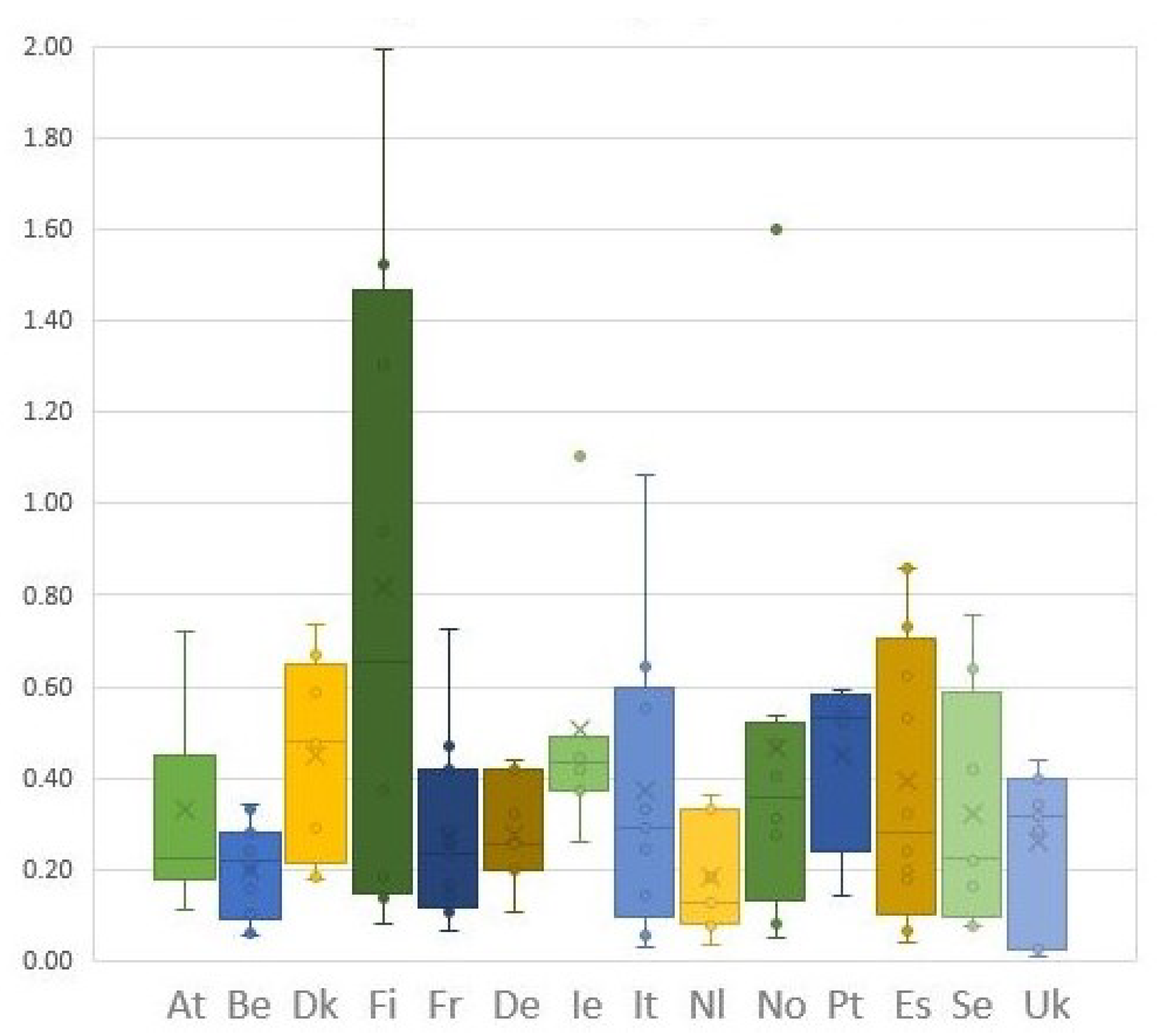
While the outliers for Ireland, Italy, and Norway constitute single party outliers in large political party systems, the three parties outliers for Finland seem to suggest a broader pattern. For a better sense of the overall disagreement between the two surveys measures at the country level, I plot the distances between the two survey estimates for each party included in a country’s survey. The box plot reported in Figure 2 displays the minimum, the first quartile, the median, the third quartile, and the maximum disagreement between the two independent surveys for each country.
Focusing on the last two quarters, that include parties with a disagreement greater than the median, we notice that the disagreement between the two survey instruments for Finnish parties is twice as much as the one for other countries. This suggests a systemic difference at the country level caused by different evaluations of the expert respondents. Such differences can be due to key changes in the country’s political environment or validity issues. It is worth noticing that Finland held parliamentary elections on 19 April 2015, between the two expert surveys. The political campaign and events occurred around the 2015 general elections constitutes important information revelation process and it is reasonable to expect that experts updated their beliefs about parties’ preferences.
Except for Finland, the results of this cross-validation test provide a strong indication that my expert survey data are not measuring something different from that of other existing and valid measures on previously analyzed dimensions, and that the respondents can indeed be considered as experts on their country’s political system.
3.2. Experts’ Agreement & Reliability
An expert survey measure is considered reliable if the experts share a certain agreement on a given dimension. Hence, low variance across the experts’ assessments of one party on a given dimension indicates that the party’s position is measured reliably.
I assess the agreement of experts’ judgments in three different ways. First, I calculate standard errors to include a measure of disagreement or uncertainty for each party rating in the dataset. Appendix reports the standard errors of the ratings of every dimension and party. Standard errors of the L-R ratings across the entire dataset are very low, with an average of 0.16 on the 21-point measurement scale. The average standard error of the other ratings ranges between 0.34 and 0.40 on the 11-point measurement scale.3
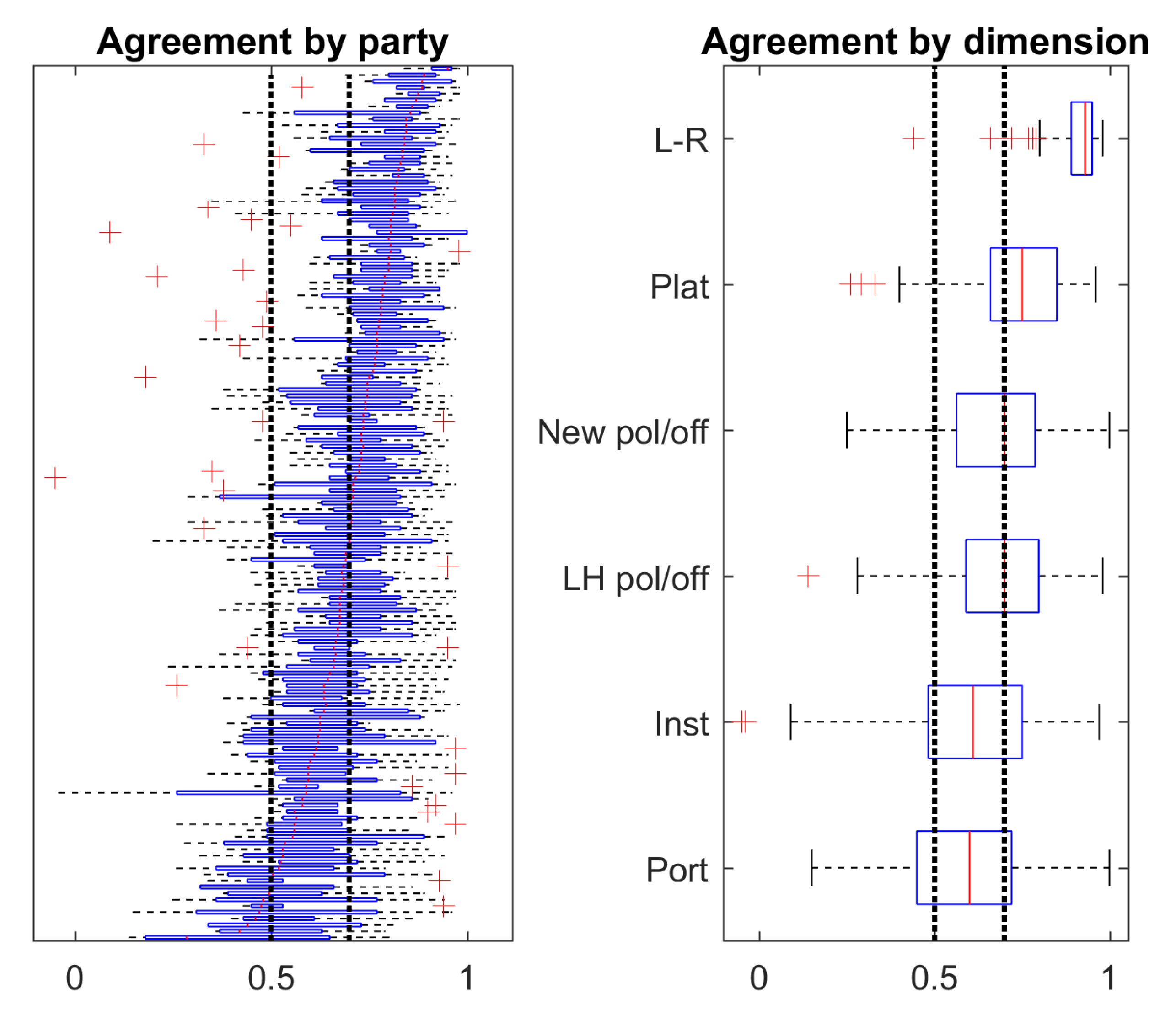
Second, I calculate the agreement rate using the measure of agreement [37]. This measure allows to overcome two drawbacks of the standard error measure. First, it provides a scale-independent measure of agreement of expert responses. Second, it accounts for expert agreement that could occur due to chance [38]. Figure 3 reports the agreement scores by parties across all dimensions (left panel) and by dimension across all parties (right panel). The two vertical lines denote the two cutoff points for acceptable (0.5) and strong (0.7) agreement.4 The left panel shoes that with very few exception, all parties display a median agreement score higher than 0.5, with more than half of them displaying strong agreement scores. The right panel indicates strong agreement across parties on all dimensions, with the exception of the Portfolio and the Institutional change dimensions that show slightly lower but still acceptable scores. The fact that the new questions introduced in this study display lower agreement scores compared to the more traditional parties’ position on the general Einstein–Bell scale is not surprising. This can be explained in at least two ways. First, experts have a presumably lower degree of familiarity with the novel questions; and second, the newly introduced dimensions have a higher degree of complexity compared to the more traditional L-R dimension.
Last, I calculate the reliability scores for every country and every dimension via the Spearman–Brown formula [39]. In Table 2 I report the reliability scores for each dimension. The reliability of the L-R ratings is greater or equal to 0.98 for every country. The reliability scores for LH off/pol, New off/pol, and Institutional change are also very high (greater than 0.94 for every country except for Finland). Portfolio show, with a few exceptions, comparable reliability scores, while the reliability scores for Platform Change are smaller and display a higher variance across countries (with a range from 0.76 to 0.98).
Across the three agreement and reliability tests, the ratings for the ratings for the left-right position (L-R) and the two ratings for the preference for policy over office (LH off/pol and New off/pol) display very high scores, implying high reliability. The three newly introduced ratings, measuring the assessment of portfolio as a means rather than an end (Portfolio), parties’ support for institutional changes (Institutional change), and parties’ willingness to change their policy platform (Platform Change) display lower but still acceptable reliability scores.5
The reliability ratings for Finland are consistently smaller than those of other countries, suggesting that the differences with the CHES expert survey that we observed for the (L-R) ratings might not be exclusively caused by changes in the political environment but rather validity of the experts’ sample.
4. Results
Parties’ preferences for policy over office are directly assessed by the LH pol/off and the New pol/off ratings.6 The scale for the LH pol/off ratings has been reversed for sake of comparison: the higher the rating is, the more the party is motivated by policy rather than office. As noted in Section 3, these two ratings differ in the framing of the questions, with the former identifying office and policy goals as incompatible objectives, and the latter construing the two goals as going hand in hand. Because the New pol/off framing eliminates the extreme scenario in which policy-motivated parties must give up offices entirely to pursue policy objectives, we expect its ratings to be higher than those for LH pol/off.
In Figure 4, I plot the New pol/off mean ratings against the LH pol/off ratings. With few exceptions, the former are always greater or equal than the latter, showing preliminary support for the claim that a framing that allows for compatibility of the two goals yields higher preferences for policy goals. I test whether the difference between the two ratings is significant using a Welch test.7 In no case is a LH pol/off rating significantly larger than a New pol/off rating, while in the majority of the cases the opposite is true.8
From an analysis of Figure 4, we notice that the effect of the new framing is not homogeneous for all countries or for all parties. Across countries, the effect of the new framing is larger and more statistically significant for parties that have more pronounced preferences for office at the expense of policy (with ratings less than 4). This suggests that for these parties, a framing that implies that purely policy motivated parties should sacrifice office entirely dramatically depresses the elicitation of policy preference. Omitting this extreme case scenario while reaffirming that policy goals could be pursued without abandoning office goals allows for a more accurate measure of the preferences for policy. As parties display higher preferences for policy goals, the new framing effect decreases, suggesting a ceiling effect.
As discussed in the previous section, it is of substantive importance for a measure of parties’ preferences to allow for the compatibility of the office and policy goals. Parties might want to control offices either because of the associated distributive perks, or because they can use office as a tool to achieve policy goals. The assumption that the goals are orthogonal would lead to the elimination of this second possible rational motive for parties to seek control over offices, and this in turn would result in the underestimation of their preference for policy goals. The observed difference in the two ratings supports this argument.
The difference in parties’ preferences that this rating produces may be a key factor especially for government formation models, in which subtle changes of preferences might generate completely different predictions. For instance, minority or surplus governments are only predicted when parties are extremely policy motivated. To have a minority government, there must be external supporters that prefer the minority government’s policy to the office perks that they could obtain by proposing an alternative coalition; surplus governments instead require government parties that prefer sharing the perks of office with extra (superfluous) parties when this leads to a better government policy [11]. In this latter case, stronger policy preferences, especially for those parties that are more likely to be in office, might be the key factor explaining why those parties are willing to enlarge the coalition.
The Value of Office: Tool or End?
In the previous section, I motivated most of the expectations as rational results of the parties’ strategic behavior: office-seeking parties would value policies as instruments to win elections, while policy-pursuing parties would be less willing to moderate on policy in order to be more competitive. In this section, I test whether these claims are supported by the survey data.
First, I test whether policy-motivated parties do indeed value office more as a tool than as an end, as measured by the Portfolio ratings. Then, I analyze whether parties’ preferences affect their support for institutional changes, as measured by the Institutional change ratings. As discussed in the previous sections, office-seeking parties are expected to act in a way that maximizes their electoral competitiveness; hence they are more likely to control offices and benefit from the status quo of a political system [4]. Policy-pursuing parties, in contrast, are less likely to compromise on their views and therefore less likely to be competitive and gain offices [40]. As a consequence, they are more likely to promote institutional changes either because these changes align with their policy views, or simply because they would allow them to achieve more successful electoral prospects.
Finally, I test the claim that parties’ preferences regarding office and policy affect their willingness to change their political platform, as measured by the Platform Change ratings. In fact, most of the formal literature assumes that for office-seeking parties policies are instruments to win elections, while for policy-pursuing parties policies are also valued in themselves. As a consequence, office-seeking parties are considered to be more likely to converge to moderate policy positions to gather greater support, while policy-pursuing parties are more likely to diverge [27,41,42].
The independent variable is the parties’ preference for policy versus office as measured by the new pol/off rating. I expect that higher ratings for policy versus office positively affect the likelihood that parties consider portfolio as a tool to achieve policy goals, their willingness to propose institutional changes, and their likelihood of staying firm on their ideological stances or getting more extreme before the elections.
In Table 3, I report the results of the three separate univariate regressions. The results confirm my hypotheses and confirm the robustness of the experts’ assessment of parties’ preferences. In every country (except Finland) the Portfolio ratings are almost perfectly explained by the new pol/off ratings (see panel A), confirming that parties that are motivated more by their policy goals than their office goals value the cabinet portfolio not per se but as a tool to accomplish policy objectives.
Except for Austria and the Netherlands, policy preferences also drive the parties’ support for the political system, with parties that are more policy motivated being more likely to propose institutional changes (panel B).
Lastly, in most countries, policy preferences also explain the parties’ decisions regarding changes to the electoral platforms, with more policy-concerned parties being less willing to moderate, but on the contrary more likely to become more rigid or even more extreme in their ideological stances (panel C).
5. Application: Government Coalition Formation
In this section, I apply the ratings for policy preferences to analyze the government formation process that took place in Spain in the aftermath of the general elections. I illustrate a simplified model of government formation based on reference [11] and use the parties’ preferences for policy and office to examine the mechanisms that led to the formation of the People’s Party minority cabinet.
The model analyzes a non-cooperative bargaining game between parties, each with a legislative seat share , where for and . Parties’ utility is function of both the cabinet portfolio allocation and the distance between the joint policy of the government coalition Z and the party’s ideal policy .9 The government policy Z is a linear combination of the policies implemented by the parties , weighted by the portfolio share they control : . Assuming that the policies outlined in the parties’ manifestos are binding, parties will implement their ideal policy once in office (). Hence, the government coalition policy is a linear combination of the coalition parties’ ideal policies weighed for their share: :
Denote party i’s utility as a quasi-linear function in which the utility is increasing in the cabinet portfolio allocation and decreasing in the distance between the government policy Z and its ideal policy .
where is a parameter that captures the policy concern of party i. The policy concern can be interpreted as a measure of how party i trades off policy closeness for office.10
The coalition formation game proceeds as follows: parties behave non-cooperatively and simultaneously propose to form a coalition with other parties. If a set of parties propose the same coalition, they move to the negotiation stage and bargain over the allocation of the cabinet portfolio. Once a consensus on the portfolio allocation is reached, they move their proposal to the floor for a vote of investiture, otherwise they terminate the negotiations.
In equilibrium, parties allocate the cabinet portfolio in a way that is proportional to the vote share that coalition parties contribute to the coalition [11,22]: . Hence, when parties propose to coalesce with other parties they look ahead and solve for the expected utility of each proposed coalition, which is function of the proportional distribution of offices and the resulting government policy.
The government formation game have multiple equilibria. However, I use the Strong Equilibrium refinement [43] to focus on equilibrium strategy profiles that are not only robust to individual deviations but also robust to improving deviations by sub-coalition of players.
A Case of Minority Government: Spain
Because of the fluidity of the political system, the survey ratings lose accuracy the longest the gap between the time in which the survey has been completed and the election held. Hence, we focus on the closest election after the conclusion of the expert survey. The 2015 Spanish elections represent a perfect case study as they take place a few weeks after the conclusion of the survey.
Parliamentary elections were held in Spain on Sunday, 20 December 2015, to elect the 350 members of the Spanish Bicameral Parliament. The number of seats won by each party is reported in the first row () of the top panel of Table 4. The incumbent, the People’s Party (PP), lost 34% of the seats in the Congress of deputies, retaining only 123 seats. The second-largest party, the Socialist Workers’ Party (PSOE), also lost 18% of the seats, retaining only 90 seats. The parties which benefited the most from the new elections were the two freshman parties: Podemos (P) and the Citizens’ Party (C’s), which entered parliament with 69 and 40 seats, respectively.
The spectacular electoral growth of Podemos and the Citizens’ Party transformed Spain’s two-party system, that characterized Spanish politics in the post-Franco period, into a fragmented multi-party system. Repeated failures to reach a government agreement resulted in a political impasse that lasted more than six months and that culminated into a call for early elections. Snap parliamentary elections were held on 26 June 2016. Podemos and United Left (IU) formed a pre-electoral coalition but, instead of gaining additional support, witnessed a surprising loss in votes compared to the previous election. The People’s Party regained some of the seats that it lost in 2015, for a total of 137 seats, but they were not enough to regain control of the majority. Overall, the new polls did not change the 2015 elections’ results: neither the right-wing (PP and C’s) nor the left-wing bloc (PSOE, P, and IU) were able to obtain an absolute majority.11 The number of seats won by each party is reported in the second row () of the top panel of Table 4.
The third and the fourth row of Panel A reports the parties’ position ratings on the general Einstein–Bell scale and the policy concerns . The policy concern captures the elasticity of substitution between policy as office and it is derived from the New pol/off ratings using a second-order Taylor expansion.12
Panel B reports the utility that each party would receive for each possible winning coalition that could form after the 2015 elections. Several permutations of parties could form a winning coalition. However, only the right-wing alliance between the People’s Party, the Citizens Party, the Democratic Convergence of Catalonia (CDC), and the Basque Nationalist Party (EAJ) (PP-C’s-CDC-EAJ) would be a Strong equilibrium of the game.
In addition, the People’s Party could also propose a minority government, which would also be a Strong Equilibrium, because no viable sub-coalition of players have an incentive to deviate. Specifically, all parties belonging to the left-wing bloc—the Socialist Workers’ Party, Podemos, the United Left, the Republican Left of Catalonia (ERC), and Amauir/EhBildu (A)—would have the incentive to form an alternative government coalition. However, no alternative government proposal would be viable without the support of either the Democratic Convergence of Catalonia or the Basque Nationalist Party. Because neither the CDC nor the EAJ would have the incentive to join the alternative coalition, as they both would prefer the People’s Party minority government than coalescing with the left-wing bloc, no deviation to depose the minority government would be viable.
Panel C reports the utility for each possible winning coalition that could form after the 2016 elections. Although the snap elections led to some changes in the parties’ seat shares, the equilibrium predictions do not substantially change. Only the right-wing coalition between PP, C’s, and the CDC would be a Strong equilibrium of the game. As before, a People’s Party minority government would also be a Strong Equilibrium. The left-wing bloc would need to coalesce with both the CDC and the EAJ to obtain a majority vote and, as before, neither of them would have an incentive to do so. For parties even moderately motivated by policy as the CDC and the EAJ, entering in a coalition with leftist parties is less appealing than been governed by an ideologically adjacent party. Because the People’s party minority government is a strong equilibrium, it is predicted to be stable, and its durability is explained by the preferences for policy of the CDC and EAJ parties.
As discussed in reference [44], after attempting different coalition agreements and seeking new majorities through snap elections, the Spanish political impasse resolved with a vote of investiture for the People’s Party minority government, which lasted until 2018. The People’s Party minority government was invested thanks to the votes of support and the abstentions of the Socialist Workers’ Party (PSOE) members, rather than the explicit support of the Democratic Convergence of Catalonia and the Basque Nationalist Party. However, I argue that the mechanism that explains the investiture and survival of the minority government lies in the lack of a credible alternative government, which required the two moderately conservative parties-the CDC and the EAJ-to join the left bloc. The theoretical model provides a counterfactual explanation of why the People’s Party emerged as the unique solution to the Spanish political impasse.
6. Conclusions
Parties’ preferences for office and policy goals are essential features of many theoretical models of party behavior. Starting with the government formation literature, which has thoroughly analyzed how different assumptions about parties’ preferences affect the type and composition of government coalitions, researchers have begun to study parties’ goals and how they affect parties’ decisions.
However, despite a few ground-breaking contributions to the study of party preferences [2,8], the literature continues to lack comprehensive and up-to-date measurements of parties’ preferences regarding policy and office objectives. This paper reports the results of an expert survey whose goal is to provide this missing measure for the study of party’s behavior.
The survey data presented in this study provide valid and reliable measures of parties preferences over different dimensions. The analyses of the survey data suggest that the party preference measurements are robust to different specifications and framing.
The paper presents an application of the preference ratings for policy versus office in the context of government formation in Spain after the 2015 elections. The Mariano Rajoy (Peoples’ Party) minority government constitutes is an equilibrium of the game because external parties such as the Democratic Convergence of Catalonia and the Basque Nationalist Party are sufficiently motivated by policy to prefer the minority government, with aligning policy position, than coalescing with parties that are farthest away on the policy spectrum. Although the Rajoy’s government obtained a vote of investiture thanks to the vote/abstention of the the Socialist Workers’ Party, the rationale that explains the investiture and survival of the minority government lies in the lack of a credible alternative government coalition that had an incentive to depose it.
As in most cross-country studies, every country is different and a unique entity. For this reason, we cannot simply apply general rules to estimate parties’ preferences, but need to keep analyzing party preferences at the country level. The present paper constitutes a first step in a thorough and comprehensive understanding of parties’ preferences. As the literature on party politics moves toward the text analysis of manifestoes to assess parties’ positions on various issues, the next step is to perform text analysis of parties’ mission statements and other secondary sources, such as parties’ convention recordings, party leaders’ addresses and interviews, and newspaper articles, to fully understand and measure parties’ preferences for office and policy goals.
Funding
This research received no external funding.
Institutional Review Board Statement
Not applicable.
Informed Consent Statement
Not applicable.
Data Availability Statement
Publicly available datasets were analyzed in this study. This data can be found here: http://bassi.web.unc.edu/data/.
Conflicts of Interest
The authors declare no conflict of interest.
Appendix A. Survey Instrument
Country experts participated in the survey during the months of October and November 2015. The country experts who were invited to complete the assessment are academics specializing in the political parties of their own country of expertise. To identify these experts, I contacted national and international political science associations with a request for their membership lists and, whenever possible, the members’ self-declared area of expertise. In those countries where a national political science association did not exist, or where the list of members of international associations yielded a less than ideal number of experts for a given country, I asked experts who participated in the survey to name additional experts and/or I consulted the directories of political science departments in search of additional experts.
An invitation to participate in the survey with a brief description of the purpose of the survey was sent by e-mail to each potential respondent between 29 October and 15 November 2015. A follow-up reminder was sent one or two weeks after the invitation. Respondents who wished to participate accessed the online survey through an individual link that allowed me to track the survey’s completion stage.
The parties included in the survey are those that had won at least one seat in the national legislature during the most recent legislative election. Furthermore, for countries with upcoming general elections (in less than 6 months from the time the survey was administered), I also included parties that were running for seats in the national legislature and that showed a sufficiently large amount of support (more than 5%) in recent non-national elections (European or local elections).
Appendix A.1. Survey Questions Script
We would like you to evaluate the current preferences and positions of the leadership of parliamentary parties in [country name]. Below you will find the logo, abbreviation, and name of all national parties (in the country language and in English).
Q: Left-Right Parties’ ideology. Please move the slider to describe each party’s overall ideology on a scale ranging from −10 (extreme left) to 10 (extreme right).
Policy vs. Office: Parties may be driven by 2 main objectives: Policy (i.e., influencing policy/advocating interests/issues/ideology) and Office (i.e., gaining executive office/cabinet portfolios). You will be asked some questions about the relative importance of these two objectives for each party.
Q: Forced to make a choice, would party leaders give up policy objectives in order to get into government OR would they sacrifice a place in government in order to maintain policy objectives? Please move the slider to describe each party’s assessment on a scale ranging from 0 (give up a place in government) to 10 (give up policy objectives).
Q: Suppose a party can form a government coalition with two alternative partners (or groups of partners). Would party leaders choose to form a coalition that gives their party the largest share of cabinet portfolios OR would they rather choose to form a coalition that would guarantee the implementation of a government policy closest to their ideal policy? Please move the slider to describe each party’s assessment on a scale ranging from 0 (largest share of cabinet portfolio) to 10 (closest government policy).
Q: Are cabinet portfolios valued more as office rewards or as means to affect policy? Please move the slider to describe each party’s assessment on a scale ranging from 0 (Cabinet portfolios are valued as an end) to 10 (Cabinet portfolios are valued as a mean).
Q: Are party leaders more likely to support the existing political system OR are they more likely to propose institutional and policy changes? Please move the slider to describe each party’s assessment on a scale ranging from 0 (Support existing political system) to 10 (Propose policy and institutional changes).
Q: Parties’ electoral political platform. Do parties change their political stances before the elections (by taking either more moderate or more extreme policies) OR are they resolute and firm on their ideological principles? Please move the slider to describe each party’s assessment on a scale ranging from -10 (Get more moderate), 0(Stay firm on ideological principles), to 10 (Get more extreme).
Appendix A.2. Ratings by Country
In Table A1 I report the average ratings for each country and each party. Furthermore, it reports the observable variables used in the regression analysis: party’s size and history.
Specifically, column 1 reports the party’s history in government as calculated by the number of days that a party has been in government over the past 16 years (from 1 January 2000, to 28 October 2015). Column 2 reports the party’s seat share. Columns 3 to 6 report the average ratings and the standard errors of the parties’ position on the general left-right position scale (‘L-R’), the parties’ preference for policy over goals assuming the two goals to be orthogonal (‘LH pol/off’), the parties’ preference for policy over goals assuming the two goals to be compatible (‘New pol/off’), the value of the cabinet portfolios (‘Port’), the parties’ support for the institutional changes (‘Inst’), and the parties’ likelihood of changing political platform (‘Plat’), respectively.

Table A1.
Mean Ratings, Seats, and History in government.
| Govt.freq | Seats | L-R | LH pol/off | New pol/off | Port | Inst | Plat | |
|---|---|---|---|---|---|---|---|---|
| AUSTRIA | ||||||||
| SPO | ||||||||
| OVP | ||||||||
| FPO | ||||||||
| GRU | ||||||||
| STR | ||||||||
| NEOS | ||||||||
| BZO | ||||||||
| BELGIUM | ||||||||
| N-VA | ||||||||
| PS | ||||||||
| CD&V | ||||||||
| VLD | ||||||||
| MR | ||||||||
| SP.A | ||||||||
| GRO | ||||||||
| CDH | ||||||||
| PVDA | ||||||||
| VB | ||||||||
| ECO | ||||||||
| FDF | ||||||||
| PP | ||||||||
| LDD | ||||||||
| DENMARK | ||||||||
| SD | ||||||||
| DF | ||||||||
| V | ||||||||
| EL | ||||||||
| LA | ||||||||
| Å | ||||||||
| RV | ||||||||
| SF | ||||||||
| C | ||||||||
| KF | ||||||||
| FINLAND | ||||||||
| KESK | ||||||||
| PS | ||||||||
| KOK | ||||||||
| SDP | ||||||||
| VIHR | ||||||||
| VAS | ||||||||
| SFP | ||||||||
| KD | ||||||||
| Å | ||||||||
| FRANCE | ||||||||
| PS | ||||||||
| PCF | ||||||||
| EELV | ||||||||
| PRG | ||||||||
| UMP | ||||||||
| NC | ||||||||
| RAD | ||||||||
| AC | ||||||||
| FDG | ||||||||
| FN | ||||||||
| MODEM | ||||||||
| GERMANY | ||||||||
| CDU | ||||||||
| SPD | ||||||||
| LINKE | ||||||||
| GRU | ||||||||
| CSU | ||||||||
| FDP | ||||||||
| AFD | ||||||||
| ICELAND | ||||||||
| S | ||||||||
| F | ||||||||
| SJ | ||||||||
| VG | ||||||||
| BF | ||||||||
| P | ||||||||
| D | ||||||||
| R | ||||||||
| IRELAND | ||||||||
| FG | ||||||||
| LAB | ||||||||
| FF | ||||||||
| SF | ||||||||
| PS | ||||||||
| PBPA | ||||||||
| WUAG | ||||||||
| G | ||||||||
| ITALY | ||||||||
| PD | ||||||||
| SEL | ||||||||
| CD | ||||||||
| PDL | ||||||||
| LN | ||||||||
| FDI | ||||||||
| M5S | ||||||||
| SC | ||||||||
| UDC | ||||||||
| NETHERLANDS | ||||||||
| VVD | ||||||||
| PVDA | ||||||||
| PVV | ||||||||
| SP | ||||||||
| CDA | ||||||||
| D66 | ||||||||
| CU | ||||||||
| GL | ||||||||
| SGP | ||||||||
| NORWAY | ||||||||
| A | ||||||||
| H | ||||||||
| FRP | ||||||||
| KRF | ||||||||
| SP | ||||||||
| V | ||||||||
| SV | ||||||||
| MDG | ||||||||
| PORTUGAL | ||||||||
| PàF | ||||||||
| PS | ||||||||
| BE | ||||||||
| CDU | ||||||||
| PSD | ||||||||
| PAN | ||||||||
| SPAIN | ||||||||
| PP | ||||||||
| PSOE | ||||||||
| P | ||||||||
| C’S | ||||||||
| IU | ||||||||
| UPyD | ||||||||
| CDC | ||||||||
| A | ||||||||
| EAJ-PNV | ||||||||
| ERC | ||||||||
| BNG | ||||||||
| CC | ||||||||
| COMPR | ||||||||
| SWEDEN | ||||||||
| SAP | ||||||||
| M | ||||||||
| SD | ||||||||
| MP | ||||||||
| C | ||||||||
| V | ||||||||
| FP | ||||||||
| KD | ||||||||
| UNITED KINGDOM | ||||||||
| CON | ||||||||
| LAB | ||||||||
| SNP | ||||||||
| LIBDEM | ||||||||
| DUP | ||||||||
| SF | ||||||||
| PLCYM | ||||||||
| SDLP | ||||||||
| UUP | ||||||||
| UKIP | ||||||||
| GRE | ||||||||
| APNI | ||||||||
In Table A2 I report the p values for the null hypothesis that the average LH pol/off rating is equal to the average New pol/off rating for each party.
Table A2.
Policy versus Office Trade-Offs.
| AT: | spo | ovp | fpo | gru | str | neos | bzo | |||||||
|---|---|---|---|---|---|---|---|---|---|---|---|---|---|---|
| LH | 1.89 | 1.85 | 3.44 | 5.41 | 1.17 | 5.00 | 1.29 | |||||||
| New | 3.00 | 2.73 | 4.64 | 6.64 | 2.67 | 5.38 | 2.37 | |||||||
| p-val | 0.000 | 0.020 | 0.014 | 0.003 | 0.003 | 0.165 | 0.090 | |||||||
| BE: | n-va | ps | cd&v | vld | mr | sp.a | gro | cdh | pvda | vb | eco | fdf | pp | ldd |
| LH | 5.48 | 2.92 | 2.24 | 3.29 | 3.00 | 3.46 | 6.60 | 3.24 | 8.32 | 8.30 | 6.40 | 6.00 | 7.62 | 7.10 |
| New | 6.87 | 3.87 | 3.46 | 4.61 | 3.79 | 4.55 | 7.54 | 4.50 | 8.45 | 7.90 | 7.58 | 5.74 | 8.58 | 7.37 |
| p-val | 0.014 | 0.002 | 0.001 | 0.000 | 0.017 | 0.001 | 0.031 | 0.000 | 0.543 | 0.827 | 0.001 | 0.248 | 0.132 | 0.738 |
| DK: | sd | df | v | el | la | å | rv | sf | c | k | ||||
| LH | 1.86 | 7.67 | 1.90 | 8.50 | 5.63 | 8.03 | 3.07 | 5.60 | 3.31 | 5.52 | ||||
| New | 3.29 | 8.59 | 3.29 | 9.21 | 7.13 | 8.72 | 5.29 | 6.43 | 5.03 | 6.79 | ||||
| p-val | 0.000 | 0.025 | 0.000 | 0.093 | 0.000 | 0.242 | 0.000 | 0.025 | 0.000 | 0.000 | ||||
| FI: | kesk | ps | kok | sdp | vihr | vas | sfp | kd | å | |||||
| LH | 2.28 | 3.06 | 2.06 | 2.61 | 5.56 | 6.28 | 2.00 | 4.38 | 4.43 | |||||
| New | 2.86 | 4.27 | 3.07 | 3.27 | 6.00 | 6.33 | 2.29 | 5.33 | 4.17 | |||||
| p-val | 0.000 | 0.000 | 0.006 | 0.008 | 0.017 | 0.197 | 0.393 | 0.076 | 0.273 | |||||
| FR: | ps | pcf | eelv | prg | ump | nc | rad | ac | fdg | fn | modem | |||
| LH | 2.17 | 6.67 | 6.10 | 3.50 | 1.90 | 2.20 | 2.89 | 2.20 | 7.21 | 6.54 | 3.71 | |||
| New | 3.00 | 6.59 | 5.90 | 4.56 | 2.69 | 3.00 | 2.63 | 3.06 | 7.69 | 7.11 | 4.36 | |||
| p-val | 0.009 | 0.733 | 0.419 | 0.008 | 0.046 | 0.000 | 0.767 | 0.000 | 0.254 | 0.283 | 0.041 | |||
| DE: | cdu | spd | linke | gru | csu | fdp | afd | |||||||
| LH | 2.36 | 3.08 | 7.32 | 5.28 | 2.97 | 2.45 | 7.45 | |||||||
| New | 3.72 | 4.44 | 7.91 | 6.70 | 4.11 | 3.59 | 8.11 | |||||||
| p-val | 0.000 | 0.000 | 0.017 | 0.000 | 0.000 | 0.000 | 0.156 | |||||||
| IS: | s | f | sj | vg | bf | p | d | r | ||||||
| LH | 2.42 | 1.25 | 3.42 | 5.50 | 4.33 | 7.27 | 6.40 | 7.25 | ||||||
| p-val | 0.000 | 0.000 | 0.000 | 0.066 | 0.078 | 0.248 | 0.014 | 1.000 | ||||||
| IE: | fg | lab | ff | sf | ps | pbpa | wuag | g | ||||||
| LH | 2.55 | 2.36 | 1.59 | 4.64 | 8.14 | 8.50 | 8.00 | 4.14 | ||||||
| New | 2.45 | 3.41 | 1.68 | 5.35 | 8.19 | 8.29 | 8.20 | 5.23 | ||||||
| p-val | 0.836 | 0.000 | 0.808 | 0.089 | 0.745 | 0.512 | 0.197 | 0.030 | ||||||
| IT: | pd | sel | cd | pdl | ln | fdi | m5s | sc | udc | |||||
| LH | 2.96 | 7.22 | 2.26 | 2.47 | 5.56 | 6.13 | 8.57 | 3.55 | 2.26 | |||||
| New | 3.48 | 7.54 | 2.70 | 2.78 | 5.68 | 5.96 | 8.45 | 4.08 | 2.98 | |||||
| p-val | 0.257 | 0.232 | 0.095 | 0.256 | 0.550 | 0.757 | 0.791 | 0.118 | 0.036 | |||||
| NL: | vvd | pvda | pvv | sp | cda | d66 | cu | gl | sgp | |||||
| LH | 2.54 | 2.27 | 6.92 | 7.27 | 1.96 | 3.74 | 6.11 | 6.04 | 7.68 | |||||
| New | 3.33 | 3.24 | 7.26 | 7.90 | 3.00 | 5.00 | 7.06 | 7.15 | 8.10 | |||||
| p-val | 0.019 | 0.000 | 0.649 | 0.042 | 0.000 | 0.000 | 0.000 | 0.000 | 0.031 | |||||
| NO: | a | h | frp | krf | sp | v | sv | mdg | ||||||
| LH | 2.00 | 2.52 | 4.67 | 5.10 | 3.57 | 5.29 | 5.05 | 6.88 | ||||||
| New | 3.20 | 4.00 | 5.33 | 6.00 | 5.47 | 6.40 | 6.60 | 8.21 | ||||||
| p-val | 0.000 | 0.000 | 0.374 | 0.011 | 0.000 | 0.001 | 0.001 | 0.010 | ||||||
| PT: | pàf | ps | be | cdu | psd | pan | ||||||||
| LH | 2.70 | 3.17 | 6.83 | 7.61 | 2.83 | 8.20 | ||||||||
| New | 3.52 | 3.91 | 7.61 | 8.43 | 3.57 | 8.22 | ||||||||
| p-val | 0.079 | 0.004 | 0.044 | 0.006 | 0.154 | 0.451 | ||||||||
| ES: | pp | psoe | p | c’s | iu | upyd | cdc | a | eaj-pnv | erc | bng | cc | compr | |
| LH | 2.19 | 2.63 | 5.33 | 3.71 | 7.12 | 4.87 | 1.92 | 6.93 | 3.19 | 4.94 | 6.24 | 2.59 | 5.89 | |
| New | 2.78 | 3.42 | 6.46 | 5.40 | 7.27 | 5.43 | 2.63 | 7.21 | 3.76 | 5.54 | 6.32 | 2.74 | 6.26 | |
| p-val | 0.046 | 0.010 | 0.000 | 0.000 | 0.845 | 0.007 | 0.002 | 0.532 | 0.068 | 0.067 | 0.840 | 0.140 | 0.271 | |
| SE: | sap | m | sd | mp | c | v | fp | kd | ||||||
| LH | 2.35 | 2.74 | 7.87 | 3.65 | 3.81 | 7.32 | 3.61 | 3.90 | ||||||
| New | 3.07 | 3.67 | 8.44 | 6.04 | 5.81 | 7.85 | 5.56 | 6.04 | ||||||
| p-val | 0.001 | 0.003 | 0.027 | 0.000 | 0.000 | 0.425 | 0.000 | 0.000 | ||||||
| UK: | con | lab | snp | libdem | dup | sf | pc | sdlp | uup | ukip | gre | apni | ||
| LH | 2.44 | 4.37 | 5.30 | 2.51 | 4.76 | 5.47 | 6.06 | 4.34 | 6.03 | 6.80 | 7.66 | 4.33 | ||
| New | 2.49 | 4.05 | 5.60 | 4.54 | 4.90 | 5.62 | 6.65 | 5.52 | 5.75 | 6.42 | 8.22 | 5.39 | ||
| p-val | 0.943 | 0.389 | 0.258 | 0.000 | 0.388 | 0.672 | 0.149 | 0.011 | 0.270 | 0.462 | 0.139 | 0.028 |
Notes: Each panel reports the mean score for the LH pol/off measure, the mean score for the New pol/off measure, and the p value for the null hypothesis that the average LH pol/off rating is equal to the average New pol/off rating for each party.
Appendix B. Explaining Parties’ Preferences
In this section I analyze whether parties’ observable characteristics may help to explain the office and policy preferences measured in the survey with the New pol/off rating. The purpose of this analysis is twofold. On the one hand, this allows us to understand the mechanism through which party preferences affect certain parties’ characteristics. One the other hand, should there be a set of characteristics that explain the variance among parties’ preferences sufficiently well, this would provide a readily available instrument for estimating parties’ preferences at any point in time.
Ref. [45] shows that a party’s size and policy moderation have a significant and positive effect on parties’ preferences for office as measured by LH. Larger and centrally positioned parties are generally more office seeking than smaller parties. These patterns can be explained by the rationality of office-seeking and policy-pursuing parties. For the former, policies are mere instruments to win elections: office-motivated parties are more likely to moderate their policy positions in order to attract more voters. By doing this, they become more competitive and successful in the general elections and consequently increase in size. For the latter, in contrast, policies are valued in themselves. Policy-motivated parties are more reluctant to change and moderate their policy positions, even knowing that by not altering their position they could lose or decrease their appeal to voters.
In addition to party size and policy position, one can argue that party history is also an important factor in explaining policy and office preferences. It is reasonable to expect parties with a long history in office to care more about office goals than policy goals relative to parties that have been confined to the opposition. The history of the political game may affect parties’ beliefs and preferences. For instance, parties in government might update their beliefs in terms of the policy power that controlling a ministry conveys; on the other hand, parties in the opposition might learn how to achieve policy goals from outside the cabinet. Or parties involved in government negotiations might learn how to bargain better to gain a larger share of government portfolio. To summarize, I expect that the longer a party has been in office, the more the party will want to remain in office.
Because the experience of a party is crucially defined by being in office or in opposition, I use the frequency with which a party has been in government as a proxy for its history. To operationalize the frequency, I construct a variable (govtfreq) that counts the number of days that a party has been in government over the previous 16 years.13 The interval of 16 years is long enough to allow for a party history that spans at least three legislatures, without tracing back to periods that might involve significantly different sociopolitical institutions and entities. While most of the parties currently sitting in the legislature were founded before 2000 and have histories much longer than 16 years, some other parties are the result of mergers, splinters, or rebranding of old parties, or are brand-new entities. While the longer-lived parties represent the ideal cases for our analysis, the others require some degree of subjective analysis. To maximize the extent to which the variable govtfreq captures the past history of a party, I include the past experience in government for those parties that are the outcome of renaming/rebranding as well as for those parties that are the result of mergers. However, I do not include the past history of splinter parties, because when a faction parts from a mother party, it strives to constitute a new entity with the goal of departing and differentiating from the mother party’s history.
To test whether a party’s size, policy position, and past history in office explain its preferences for office and policy goals, I run a series of univariate regression analyses (for every country under consideration and each variable) using the parties as the units of analysis. The variable seats denotes the proportion of seats controlled by a party in the current legislature and takes a value between 0 and 1. The variable abs(position) denotes the extremeness of a party’s policy position on the general left-right continuum, and it is calculated as the absolute value of the L-R rating, taking a value between 0 and 10. Last, the variable govtfreq denotes the frequency with which a party has been in government over the previous 16 years and takes a value between 0 (never) and 1 (always). The dependent variable is the party preference for policy versus office as measured by the new pol/off rating. In Table A3 I report the results of the three univariate analyses.
While in most countries at least one of the three independent variables is significant and able to explain most of the difference in the parties’ policy and office preferences, in a few countries (notably Austria, Finland, and Italy) parties’ preferences cannot be explained by any of three proposed factors. In all other countries, the effect of the three factors is in the expected direction, with longer history in office and larger size negatively affecting parties’ preferences for policy, and more extreme policy preferences positively affecting parties’ preferences for policy.
Table A3.
Explaining the Preference Parameter (Univariate Regressions).
| at | be | de | dk | es | fi | fr | ie | is | it | nl | no | pt | se | uk | |
|---|---|---|---|---|---|---|---|---|---|---|---|---|---|---|---|
| govtfreq | |||||||||||||||
| Adj. | |||||||||||||||
| abs(position) | |||||||||||||||
| Adj. | |||||||||||||||
| seats | −13.77 | ||||||||||||||
| Adj. |
Notes: Each panel reports the coefficient estimates, the t statistics, the , and the adjusted for every party for the govtfreq, the abs(position) and the seats variables. A indicates 5% significance, while a indicates 1% significance.
Furthermore, there is a substantial heterogeneity in the specific factors that are more relevant in explaining parties’ policy versus office preferences. While the factor that explains most of the variance among parties’ preferences in the majority of the countries is the past history in office (Belgium, Denmark, Germany, Ireland, the Netherlands, Portugal, and Sweden), in other countries it is the party’s policy extremeness (France and Spain) or the seats controlled by the party (Iceland, Norway, and UK).
In Table A4, I check whether the introduction of an additional explanatory variable increases the fit of the parties’ preferences. Indeed, the fit increases in every country as documented by the adjusted , indicating that the use of multiple variables can explain up to 97% of the variation of the parties’ preferences.
Table A4.
Explaining the Preference Parameter (Bivariate Regressions).
| at | be | de | dk | es | fi | fr | ie | is | it | nl | no | pt | se | uk | |
|---|---|---|---|---|---|---|---|---|---|---|---|---|---|---|---|
| govtfreq | |||||||||||||||
| abs(position) | |||||||||||||||
| Adj. | |||||||||||||||
| govtfreq | |||||||||||||||
| seats | |||||||||||||||
| Adj. | |||||||||||||||
| abs(position) | |||||||||||||||
| seats | |||||||||||||||
| Adj. |
Notes: Each panel reports the coefficient estimates, the t statistics, the , and the adjusted for every party for every combination of two variables. The first panel reports the results for the model that includes govtfreq and abs(position). The second panel reports the results for the model that combines govtfreq and seats. The third panel presents the results of the model that includes abs(position) and seats. A indicates 5% significance, while a indicates 1% significance.
These results show that parties’ preferences can be accounted for by a set of observable variables. This is important because the use of the loadings reported in Table A3 and Table A4 can help researchers to obtain a real-time updated estimates of parties’ preference parameters, which can be used in theoretical models to make predictions about government formation.
Note also that the estimated coefficients on this set of observable variables are not identical in the cross-section of countries. This suggests that these coefficients could also vary in the time-series dimension. To validate this hypothesis, additional surveys will need to be conducted at regular time intervals.
References
- Laver, M.; Schofield, N. Multiparty Governments: The Politics of Coalitions in Europe; University of Michigan Press: Ann Arbor, MI, USA, 1990. [Google Scholar]
- Harmel, R.; Janda, K. An Integrated Theory of Party Goals and Party Change. J. Theor. Politics 1994, 6, 259–287. [Google Scholar] [CrossRef]
- Warwick, P.V. Policy Horizons and Parliamentary Government; Palgrave: New York, NY, USA, 2006. [Google Scholar]
- Anderson, C.J.; Just, A. Legitimacy from above: The partisan foundations of support for the political system in democracies. Eur. Political Sci. Rev. 2014, 5, 335–362. [Google Scholar] [CrossRef] [Green Version]
- Downs, A. An Economic Theory of Democracy; Harper and Row: New York, NY, USA, 1957. [Google Scholar]
- Wittman, D. Parties as Utility Maximizers. Am. Political Sci. Rev. 1973, 67, 490–498. [Google Scholar] [CrossRef]
- Sened, I. A Model of Coalition Formation: Theory and Evidence. J. Politics 1996, 58, 350–372. [Google Scholar] [CrossRef]
- Laver, M.; Hunt, B.H. Policy and Party Competition; Routledge Press: New York, NY, USA, 1992. [Google Scholar]
- Laver, M.; Shepsle, K. Making and Breaking Governments: Cabinets and Legislatures in Parliamentary Democracies; Cambridge University Press: Cambridge, MA, USA, 1996. [Google Scholar]
- Indriðason, I.H.; Kristinsson, G.H. Making Words Count: Coalition Agreements and Cabinet Management. Eur. J. Political Res. 2013, 52, 822–846. [Google Scholar] [CrossRef]
- Bassi, A. Policy Preferences in Coalition Formation and the Stability of Minority and Surplus Governments. J. Politics 2017, 79, 250–268. [Google Scholar] [CrossRef]
- Riker, W. The Theory of Political Coalitions; Yale University Press: New Haven, CT, USA, 1962. [Google Scholar]
- Axelrod, R. Conflict of Interest; Markham: Chicago, IL, USA, 1970. [Google Scholar]
- De Swaan, A. Coalition Theories and Cabinet Formation; Elsevier: Amsterdam, NL, USA, 1973. [Google Scholar]
- Gamson, W. A Theory of Coalition Formation. Am. Sociol. Rev. 1961, 26, 373–382. [Google Scholar] [CrossRef]
- Martin, L.W.; Stevenson, R.T. Government Formation in Parliamentary Democracies. Am. J. Political Sci. 2001, 45, 33–50. [Google Scholar] [CrossRef]
- Martin, L.W.; Stevenson, R.T. The Conditional Impact of Incumbency on Government Formation. Am. Political Sci. Rev. 2010, 104, 503–518. [Google Scholar] [CrossRef] [Green Version]
- Martin, L.W.; Vanberg, G. Wasting Time? The Impact of Ideology and Size on Delay in Coalition Formation. Br. J. Political Sci. 2003, 33, 323–332. [Google Scholar] [CrossRef] [Green Version]
- Von Neumann, J.; Morgenstern, O. Theory of Games and Economic Behavior; Princeton University Press: Princeton, NJ, USA, 1953. [Google Scholar]
- Austen-Smith, D.; Banks, J. Elections, Coalitions, and Legislative Outcomes. Am. Political Sci. Rev. 1988, 82, 405–422. [Google Scholar] [CrossRef]
- Baron, D.P.; Ferejohn, J. Bargaining in Legislatures. Am. Political Sci. Rev. 1989, 83, 1181–1206. [Google Scholar] [CrossRef] [Green Version]
- Bassi, A. A Model of Endogenous Government Formation. Am. J. Political Sci. 2013, 57, 777–793. [Google Scholar] [CrossRef]
- Morelli, M. Demand Competition and Policy Compromise in Legislative Bargaining. Am. Political Sci. Rev. 1999, 93, 809–820. [Google Scholar] [CrossRef] [Green Version]
- Baron, D.P.; Diermeier, D. Elections, Governments, and Parliaments under Proportional Representation. Q. J. Econ. 2001, 116, 933–967. [Google Scholar] [CrossRef]
- Crombez, C. Minority Governments, Minimal Winning Coalitions and Surplus Majorities in Parliamentary Systems. Eur. J. Political Res. 1996, 29, 1–29. [Google Scholar] [CrossRef]
- Diermeier, D.; Merlo, A. Government Turnover in Parliamentary Democracies. J. Econ. Theory. 2000, 94, 46–79. [Google Scholar] [CrossRef] [Green Version]
- Sánchez-Cuenca, I. Party Moderation and Politicians’ Ideological Rigidity. Party Politics 2004, 10, 325–342. [Google Scholar] [CrossRef] [Green Version]
- Giannetti, D.; Sened, I. Party Competition and Coalition Formation: Italy 1994–96. J. Theor. Politics 2004, 16, 483–515. [Google Scholar] [CrossRef]
- Shikano, S.; Linhart, E. Coalition-Formation as a Result of Policy and Office Motivations in the German Federal States: An Empirical Estimate of the Weighting Parameters of Both Motivations. Party Politics 2010, 16, 111–130. [Google Scholar] [CrossRef] [Green Version]
- Harmel, R.; Janda, K. The Party Change Project. Available online: https://liberalarts.tamu.edu/pols/research/data-resources/party-change-project/ (accessed on 1 January 2021).
- Bäck, H.; Debus, M.; Dumont, P. Who Gets What in Coalition Governments? Predictors of Portfolio Allocation in Parliamentary Democracies. Eur. J. Political Res. 2011, 50, 441–478. [Google Scholar] [CrossRef]
- Bakker, R.; de Vries, C.; Edwards, E.; Hooghe, L.; Jolly, S.; Marks, G.; Polk, J.; Rovny, J.; Steenbergen, M.; Vachudova, M.A. Measuring party positions in Europe: The Chapel Hill Expert Survey trend file, 1999–2010. Party Politics 2015, 21, 143–152. [Google Scholar] [CrossRef]
- Hooghe, L.; Bakker, R.; Brigevich, A.; de Vries, C.; Edwards, E.; Marks, G.; Rovny, J.; Steenbergen, M.; Vachudova, M.A. Reliability and validity of the 2002 and 2006 Chapel Hill expert surveys on party positioning. Eur. J. Political Res. 2010, 49, 687–703. [Google Scholar] [CrossRef] [Green Version]
- Marks, G.; Hooghe, L.; Steenbergen, M.; Bakker, R. Cross-Validating Data on Party Positioning on European Integration. Elect. Stud. 2007, 26, 23–38. [Google Scholar] [CrossRef]
- Whitefield, S.; Vachudova, M.A.; Steenbergen, M.; Rohrschneider, R.; Marks, G.; Loveless, M.P.; Hooghe, L. Do expert surveys produce consistent estimates of party stances on European integration? Comparing expert surveys in the difficult case of Central and Eastern Europe. Elect. Stud. 2007, 26, 50–61. [Google Scholar] [CrossRef]
- Benoit, K.; Laver, M. Party Policy in Modern Democracies; Routledge: New York, NY, USA, 2006. [Google Scholar]
- Finn, R.H. A note on estimating the reliability of categorical data. Educ. Andpsychol. Meas. 1970, 30, 71–76. [Google Scholar] [CrossRef]
- Lindstädt, R.; Proksch, S.O.; Slapin, J.B. When Experts Disagree: Response Aggregation and Its Consequences in Expert Surveys. Political Sci. Res. Methods. 2020, 8, 580–588. [Google Scholar] [CrossRef]
- Steenbergen, M.R.; Marks, G. Evaluating expert judgments. Eur. J. Political Res. 2007, 46, 347–366. [Google Scholar] [CrossRef]
- Strøm, K. A behavioral theory of competitive parties. Am. J. Political Sci. 1990, 34, 565–598. [Google Scholar] [CrossRef]
- Alesina, A.; Rosenthal, H. Partisan Politics, Divided Government, and the Economy; Cambridge University Press: Cambridge, UK, 1995. [Google Scholar]
- Roemer, J. Political Competition. Theory and Applications; Harvard University Press: Cambridge, MA, USA, 2001. [Google Scholar]
- Aumann, R.J. Acceptable Points in General Cooperative n-Person Games. In Contributions to the Theory of Games IV, Annals of Mathematical Studies 40; Tucker, A.W., Luce, R.D., Eds.; Princeton University Press: Princeton, NJ, USA, 1988; pp. 287–324. [Google Scholar]
- Simón, P. The Challenges of the New Spanish Multipartism: Government Formation Failure and the 2016 General Election. South Eur. Soc. Politics 2016, 21, 493–517. [Google Scholar] [CrossRef] [Green Version]
- Pedersen, H.H. What do Parties Want? Policy versus Office. West Eur. Politics 2012, 35, 896–910. [Google Scholar]
| 1. | |
| 2. | For this question, we use a 21-point scale to capture the direction of platform change. The question asks respondents: Do parties change their political stances before the elections (by taking either more moderate or more extreme policies) OR are they resolute and firm on their ideological principles? Please move the slider to describe each party’s assessment on a scale ranging from −10 (Get more moderate), 0(Stay firm on ideological principles), to 10 (Get more extreme). |
| 3. | The Platform change ratings show comparable standard errors: an average of 0.60 on the 21-point measurement scale. |
| 4. | Scores greater than 0.7 indicate strong agreement, while scores less than 0.5 indicate low agreement [38]. |
| 5. | Notice that the Platform Change question asks respondents two things at the same time: if parties change political platform and, if so, in which direction. The compression of two questions in one could have caused some confusion to the experts and thus less reliable ratings. |
| 6. | The mean ratings for all dimensions, along with their standard errors, are presented in the appendix. |
| 7. | I test the null hypothesis that the average LH pol/off rating () is equal to New pol/off rating () |
| 8. | |
| 9. | The parties’ ideal policy, , is outlined in the parties’ manifesto and is consequently common knowledge. |
| 10. | If is equal to 1, policy closeness and office affect the utility of party i equally. If is less than 1, party i requires more than a unit of policy closeness to trade off for a unit of office. In other words, party i is motivated more by office than by policy. The opposite occurs when is greater than 1. |
| 11. | A coalition needs to control at least 176 of the 350 seats to win an investiture vote. |
| 12. | The New pol/off ratings are re-scaled to measure the importance of policy vs. office in a [0,1] interval (). The policy concern describes the elasticity of substitution between policy as office in a utility function of the type . Hence, can be approximated to . Because is a convex function, I use a second-order Taylor expansion to estimate the parameter : , where and . |
| 13. | From 1 January 2000, through to 28 October 2015, after which time the survey started being administered. |
Figure 1.
Parties’ left–right estimates versus Chapel Hill Expert Survey (CHES) 2015 mean scores.

Figure 2.
Disagreement in parties’ Left–Right position estimates.

Figure 3.
Agreement scores of the experts responses.

Figure 4.
Parties’ policy-office preferences, by country.

Table 1.
The Policy vs. Office Goals Survey.
| Country | Number of Parties | Number of Respondents |
|---|---|---|
| Austria | 7 | 28 |
| Belgium | 14 | 25 |
| Denmark | 10 | 42 |
| Finland | 9 | 19 |
| France | 11 | 30 |
| Germany | 7 | 127 |
| Iceland | 8 | 12 |
| Ireland | 8 | 22 |
| Italy | 9 | 52 |
| Luxembourg | 7 | 3 |
| Netherlands | 9 | 27 |
| Norway | 8 | 21 |
| Portugal | 6 | 23 |
| Spain | 13 | 53 |
| Sweden | 8 | 32 |
| United Kingdom | 12 | 43 |
| 15 countries | 137 parties | 559 respondents |
Notes: The table reports the countries included in the survey, the number of parties for each country, and the number of respondents who completed the survey.
Table 2.
Reliability of the Policy versus Office Goals Survey.
| Country | L-R | LH | New | Portfolio | Institutional | Platform |
|---|---|---|---|---|---|---|
| Position | pol/off | pol/off | Change | Change | ||
| Austria | ||||||
| Belgium | ||||||
| Denmark | ||||||
| Finland | ||||||
| France | ||||||
| Germany | ||||||
| Iceland | ||||||
| Ireland | ||||||
| Italy | ||||||
| Netherlands | ||||||
| Norway | ||||||
| Portugal | ||||||
| Spain | ||||||
| Sweden | ||||||
| United Kingdom |
Notes: The table reports the Spearman–Brown reliability score for the variables included in the survey: Einstein–Bell (LR), Laver and Hunt policy/office tradeoff (LH pol/off ), new policy/office tradeoff preference (New pol/off), portfolio desirability (Portfolio), institutional change (Institutional Change), and Platform change (Platform Change).
Table 3.
Explaining Portfolio value, Institutional Change, and Platform Change.
| Panel A: Portfolio value is the Dependent Variable | |||||||||||||||
| at | be | de | dk | es | fi | fr | ie | is | it | nl | no | pt | se | uk | |
| New pol/off | |||||||||||||||
| Adj. | |||||||||||||||
| Panel B: Institutional Change is the Dependent Variable | |||||||||||||||
| at | be | de | dk | es | fi | fr | ie | is | it | nl | no | pt | se | uk | |
| New pol/off | |||||||||||||||
| Adj. | |||||||||||||||
| Panel C: Platform Change is the Dependent Variable | |||||||||||||||
| at | be | de | dk | fi | fr | ie | is | it | nl | no | pt | es | se | uk | |
| New pol/off | |||||||||||||||
| Adj. | |||||||||||||||
Notes: Each panel reports the coefficient estimates of the New pol/off variable, the t statistics, the , and the adjusted for every party for the models explaining cabinet portfolio value, institutional change, and platform change. A indicates 5% significance, while a indicates 1% significance.
Table 4.
Spain 2015–2016.
| Panel A: Parties’ size and preference parameters | ||||||||||
|---|---|---|---|---|---|---|---|---|---|---|
| pp | psoe | p | c’s | iu | cdc | eaj | erc | cc | a | |
| 123 | 90 | 69 | 40 | 2 | 8 | 6 | 9 | 1 | 2 | |
| 137 | 85 | 69 | 32 | 2 | 8 | 5 | 9 | 1 | 2 | |
| 0.79 | 0.39 | 0.19 | 0.64 | 0.17 | 0.69 | 0.65 | 0.28 | 0.61 | 0.19 | |
| 0.47 | 0.62 | 2.84 | 1.72 | 4.55 | 0.48 | 0.80 | 1.78 | 0.48 | 4.63 | |
| Panel B: Coalition formation 2015 | ||||||||||
| Coalitions | ||||||||||
| pp-cs-cdc-eaj | 1.15 | 0.40 | 1.24 | 1.76 | 1.91 | 0.49 | 0.76 | 0.95 | 0.41 | 1.98 |
| psoe-p-iu-eaj-erc-a | 0.25 | 1.08 | 2.88 | 1.15 | 3.86 | 0.29 | 0.56 | 1.75 | 0.34 | 3.98 |
| psoe-p-iu-cdc-erc-a | 0.25 | 1.07 | 2.86 | 1.16 | 3.82 | 0.34 | 0.53 | 1.74 | 0.34 | 3.96 |
| pp | 1.47 | 0.37 | 1.12 | 1.46 | 1.71 | 0.43 | 0.69 | 0.87 | 0.40 | 1.78 |
| Panel C: Coalition formation 2016 | ||||||||||
| Coalitions | ||||||||||
| pp-cs-cdc | 1.23 | 0.39 | 1.21 | 1.70 | 1.85 | 0.49 | 0.72 | 0.93 | 0.40 | 1.92 |
| psoe-p-iu-cdc-eaj-erc-a | 0.25 | 1.05 | 2.84 | 1.17 | 3.86 | 0.19 | 0.56 | 1.76 | 0.34 | 3.71 |
| pp | 1.47 | 0.37 | 1.12 | 1.46 | 1.71 | 0.43 | 0.69 | 0.87 | 0.40 | 1.78 |
pp = People’s Party; psoe = Socialist Workers’ Party; p = Podemos; c’s = Citizens Party; iu = United Left; cdc = Democratic Convergence of Catalonia; eaj = Basque Nationalist Party; erc = Republican Left of Catalonia; cc = Canarian Coalition; a = Amauir/EhBildu.
Publisher’s Note: MDPI stays neutral with regard to jurisdictional claims in published maps and institutional affiliations. |
© 2021 by the author. Licensee MDPI, Basel, Switzerland. This article is an open access article distributed under the terms and conditions of the Creative Commons Attribution (CC BY) license (http://creativecommons.org/licenses/by/4.0/).
Share and Cite
MDPI and ACS Style
Bassi, A. Parties’ Preferences for Office and Policy Goals. Games 2021, 12, 6. https://0-doi-org.brum.beds.ac.uk/10.3390/g12010006
AMA Style
Bassi A. Parties’ Preferences for Office and Policy Goals. Games. 2021; 12(1):6. https://0-doi-org.brum.beds.ac.uk/10.3390/g12010006
Chicago/Turabian StyleBassi, Anna. 2021. "Parties’ Preferences for Office and Policy Goals" Games 12, no. 1: 6. https://0-doi-org.brum.beds.ac.uk/10.3390/g12010006
Note that from the first issue of 2016, this journal uses article numbers instead of page numbers. See further details here.