Necessary Optimality Conditions for a Class of Control Problems with State Constraint


Faculty of Electrical Engineering, Automatics, Computer Science and Biomedical Engineering, AGH University of Science and Technology, al. Mickiewicza 30, 30-059 Kraków, Poland
*
Author to whom correspondence should be addressed.
Games 2021, 12(1), 9; https://0-doi-org.brum.beds.ac.uk/10.3390/g12010009
Submission received: 23 November 2020
/
Revised: 7 January 2021
/
Accepted: 13 January 2021
/
Published: 18 January 2021
(This article belongs to the Special Issue Optimal Control Theory)
Abstract
:An elementary approach to a class of optimal control problems with pathwise state constraint is proposed. Based on spike variations of control, it yields simple proofs and constructive necessary conditions, including some new characterizations of optimal control. Two examples are discussed.
1. Introduction
Necessary optimality conditions for control problems with pathwise state constraints have been widely studied since the beginnings of optimal control theory [1], and this domain of research is still vivid nowadays [2]. Most of the existing approaches may be divided into two streams [3]. The first one, characterized by the use of classical methods of analysis with often heuristic proofs, yields results of limited generality (see the review [4], and [3]). The other is based on the abstract theory of infinite-dimensional optimization and its results encompass a wide class of problems, with rigorous but demanding proofs (see [5,6,7,8,9]). However, these results are difficult for practical verification, because of too general characterizations of the adjoint variables and multiplier functions. Generally, the existing approaches are hardly constructive, meaning they do not give sufficient indications how to improve a nonoptimal control.
We propose an elementary approach to necessary optimality conditions for problems in Mayer form with free final state and a scalar state constraint. The controls are scalar functions and nontangentiality is assumed at all entry and exit points. As is well known, the proof of the minimum principle with free final state and without pathwise state constraints can be made elementary and simple by considering the cost increment caused by a single spike variation of control. Our first purpose is to show that a similar proof technique may be effective when a pathwise state constraint is present, with the difference that additionally a coordinated pair of spikes is used. A second purpose is to extend the known results for state constraints of index one, mainly to nonregular problems in which the optimal control and the corresponding state trajectory may at the same time take values on the boundaries of their respective admissible sets. In particular, we allow for discrete sets of admissible control values. From a conceptual point of view, this work also offers a clear geometrical interpretation of the results. On the practical side, an advantage of our approach is that the obtained conditions are readily verifiable and constructive: if they are not fulfilled, a gradient optimization procedure can be indicated and initialized which guarantees an improvement of the control, up to numerical precision (as in the method of Monotone Structural Evolution [10]). Of course, the other approaches clearly prevail in a wider perspective, when problems of greater complexity are also taken into account. They then produce optimality conditions, which can be effectively used in optimal control computations (see [11,12,13,14]).
Consider a control system described by a state equation
with a given initial condition and a given time horizon T. The controls are piecewise continuous functions of time, taking values in a given set U, that is, they belong to . 1 The function is of class in its both arguments. We make a general assumption that all solutions of (1) appearing in the sequel are well defined in the whole time interval . The state is subject to a scalar pathwise constraint,
The function is of class , and if . We assume . A performance index (or cost),
is minimized on the trajectories of (1). The function is of class .
For a control , let x be the corresponding solution of the initial value problem (1). The control u is admissible if the trajectory x satisfies the state constraint (2). The control u is optimal if it is admissible and minimizes the cost Q in the set of all admissible controls. A boundary interval of u is defined as any nonempty and right-open interval of time in which . Any nonempty and right-open interval of time, such that for every t in that interval, is nonboundary. If is an inclusion-maximal boundary interval of u and , then is called an entry point of u. If , then is an exit point. Denote
The derivative of the function along the trajectories of (1) is equal to .
For admissible controls we introduce the concept of verifiability, aiming to distinguish the controls to which the spike technique of (non)optimality verification, developed below, can be effectively applied. Let u be an admissible control with the corresponding state trajectory x. We call this control verifiable if
- (i)
- it has a finite number of inclusion-maximal boundary intervals,
- (ii)
- an implication holds that if for a certain t, then t belongs to the closure of some boundary interval of u, 2
- (iii)
- the conditions of nontangentiality
- (iv)
- there is an open set containing all points such that , and there is a function such that
2. The One-Spike Control Variation and Trajectory Variation
Let u be a verifiable control, and x, the corresponding state trajectory. Denote
For any , any , and any sufficiently small , we shall define a control . We also define as the solution of the initial value problem
We put if , and if . To define for , suppose first that . Then
- (i)
- if for some , and u has no exit points in ,
- (ii)
- if and , where is the greatest entry point of u less than or equal to t,
- (iii)
- otherwise.
Let now belong to , an inclusion-maximal boundary interval of u, and . Then for , and (i), (ii), (iii) are valid for .
The spike variation of control is the difference . Note that the control is admissible for every sufficiently small positive .
Lemma 1.
The trajectory incrementsatisfies
for every, where the trajectory variationis absolutely continuous except, possibly, at the entry points of u, and independent of. For almost every
moreover,
and at every entry pointof u
Here
Proof.
If the control u has no entry points in , the lemma is obviously true by virtue of the classical theorems on ordinary differential equations. Suppose that u has exactly one entry point in . From the mentioned theorems it directly follows that (5) holds in the time interval , with an absolutely continuous function , satisfying (7) and (6) in that interval. We shall prove that the relationships (5) and (6) may be extended to the whole interval , with the function absolutely continuous in . To this end, let us first notice that for every sufficiently small the control has an entry point , where is a real number independent of . This follows from the verifiability of u (see (4)) and from the construction of . Let . To fix attention, assume . We then have
as . Hence
By the definition of entry points, . Thus
and so
Substituting this into (10), we obtain
As and , we get
Defining by (8), we arrive at the extension of (5) and (6) to because of the same classical theorems on differential equations. For , an analogous argument leads to the same result. The proof can be easily generalized to an arbitrary finite number of entry points. □
3. The Adjoint Function and The One-Spike Necessary Optimality Condition
As in Section 2, let u be a verifiable control and x, the corresponding solution of (1). With every such control we associate an adjoint function , defined as a solution of the adjoint equation
absolutely continuous except at the entry points of u and satisfying the final condition
At every entry point , and
Let be an arbitrary point from , and , the trajectory variation determined in Lemma 1. It is easy to notice that the function is constant in the whole time interval . Indeed, its derivative equals zero at every t where and are differentiable, and at the entry points we have by virtue of (13) and (8): . Thus,
Define the pre-Hamiltonian , , and its increment
for any and (note that is only defined for a uniquely predetermined control u). We can now express the value of cost on the control , defined in Section 2
A sufficient condition for the existence of spike variations which improve the cost is a straightforward consequence.
Lemma 2.
Assume that, , and. Then the controlis admissible andfor every sufficiently small.
A theorem on optimal control of the minimum principle type follows from Lemma 2.
Theorem 1.
Assume that the control u is optimal. Then:
- (i)
- for everyand every,
- (ii)
- the functionis constant.
Proof.
Conclusion (i) is a direct consequence of Lemma 2. Conclusion (ii) for the nonboundary intervals is proved exactly as in the classical proofs of the minimum principle without pathwise state constraints. In the interior of every boundary interval, the function is of class with the derivative identically zero. The continuity of at entry points readily follows from (13) and (9). Let now be an exit point of u. By (i) and (4), there is a such that for all , and for all . The continuity of at is shown by limit passages: for the first of these inequalities, and for the second. □
Corollary 1.
Assume that the control u is optimal andfor some. Thenorfor every.
4. The Two-Spike Necessary Optimality Condition
For a verifiable control u and the corresponding state trajectory x, we shall define a two-spike control variation. Let be an inclusion-maximal boundary interval of u. For any quintuple such that , , , , and for any sufficiently small we define a control (not to be confused with the control defined in Section 2) and the corresponding state trajectory . We put if , if , if , and for any other t in . Points (i), (ii) and (iii) of the definition in Section 2 apply to all the remaining values of t. The two-spike control variation is the difference .
The control u may sometimes be improved even if it fulfills the necessary optimality condition (i) of Theorem 1. We shall now give conditions, sufficient for the existence of a two-spike control variation in which is admissible and guarantees a cost improvement.
Lemma 3.
Assume that, , , , and
Then for every sufficiently smallthe controlis admissible, and.
Proof.
It follows from the definition of and the inequalities (15), (16) that for every sufficiently small the function is negative in the time interval and constant in the intervals and ,
From this we infer that the control is admissible for all sufficiently small . Reasoning similarly as in Section 3 and using the adjoint function defined therein, we estimate the value of the performance index on the control .
Hence, (17) is a sufficient condition for the two-spike control variation to reduce the cost for every sufficiently small . □
Lemma 4.
Assume that, , , and
Assume also that if, then
Under these assumptions there is an, such that for every sufficiently smallthe controlis admissible, and.
Proof.
We shall show that the assumptions of Lemma 3 follow from the assumptions of Lemma 4. Denote
Of course and . The inequality (15) is obvious. In view of (18), (17) is true for every . If , then (16) holds for every , and the assumptions of Lemma 3 are satisfied. If , then the inequality (16) holds for . We thus have a two-sided bound on , . The interval of admissible values of is nonempty if , and this inequality follows from (19). □
By contradicting the sufficient nonoptimality conditions of Lemma 4 we obtain new necessary conditions of optimality.
Theorem 2 (main result).
Assume that the control u is optimal and verifiable, and has a boundary interval. Let also, , and. Under these assumptions:
- (i)
- ifand, then,
- (ii)
- ifand, then,
- (iii)
- ifand, thenand
Proof.
Let first . Suppose, contrary to (i), that , and . From Corollary 1, . By Lemma 4, this contradicts the assumption that u is optimal. The implication (ii) is similarly proved. Let , and . By Corollary 1, and the assumptions of Lemma 4 are fulfilled (with and ). To prove (iii), assume that and . It follows from Corollary 1 that and . If , the assumptions of Lemma 4 hold. If , the inequality opposite to (19), that is (20), is true.
Let now . The proof goes similarly, however, we additionally have to use a simple observation (rc): the functions and are right-continuous in for every . Let , and . By virtue of (rc) and Corollary 1, there is a such that and . Lemma 4 then gives a contradiction. To prove (ii), assume , and . By (rc) and Corollary 1, and there is a , , such that and for every . If for some , Lemma 4 again yields a contradiction. If for every , then (19) holds for every sufficiently close to , since as , and so Lemma 4 gives a contradiction. We shall now prove (iii). Let and . It follows from (rc) and Corollary 1 that and there is a , , such that and for every . If for some , a contradiction follows from Lemma 4. Similarly, Lemma 4 gives a contradiction if for some the relationships and (19) are fulfilled. In consequence, the inequalities and (20) with and hold true for every . By (rc), and as .
If , then (19) is true for all , sufficiently close to . We have thus come to a contradiction. Hence , and the inequality (20) holds by virtue of (rc). □
5. A Geometrical Interpretation and a Minimum Condition
Let u be a verifiable control with a boundary interval . The corresponding state and adjoint trajectories are denoted by x and , respectively. Define a family of sets
It readily follows from this definition that for every . In the sequel we implicitly assume that .
We shall now characterize the properties of the sets which result from control optimality. For an arbitrary nonzero vector , define as the angle between and y, measured anticlockwise and taking values in the interval . Let also
for every . Corollary 1 says that if u is optimal, then has no points in quadrant III of the coordinate system . The following theorem is a straightforward consequence of that corollary and of Theorem 2.
Theorem 3.
Assume that the control u is optimal. Then
- (i)
- for every,
- (ii)
- for every pairsuch that.
From this it easily follows that if the control u is optimal and for every , then for every , and the function is nondecreasing in .
It proves useful to describe the consequences of control optimality in terms of the straight lines supporting the sets at zero. This allows easier verification of the necessary conditions of optimality, and also expressing a partial optimality criterion as a minimum condition imposed on the extended pre-Hamiltonian. We say that a straight line is a supporting line of at the origin (SLO) if it is given by with , , and for every . Generally, the set may have many SLOs, whether the control is optimal or not. If u is optimal, then every set , , has an SLO with . The set has a unique SLO if and only if .
The equality occurs in two practically important situations (mutually nonexclusive). One of them, in which the right-hand side of the system equation (1) is affine in control, will be discussed in Section 7. Here we consider the other situation, in which has a tangent at the origin. A sufficient condition for that reads
Under this condition, the tangent has the equation with
Of course, if has both an SLO and a tangent at the origin, they coincide.
Suppose u is optimal and for every . Then every set , , has a unique SLO. The SLO is vertical if ; if , the SLO equation may be written as with a nonpositive directional coefficient . If, additionally, the condition (21) is fulfilled with , then
The function p thus defined is nondecreasing in all that part of where it is determined.
Define the extended pre-Hamiltonian . If the control u is optimal and the function p is determined as above in all the interval , then the following minimum condition is straightforward by the properties of SLO
This necessary optimality condition is similar to the minimum condition of indirect adjoining. We postpone a discussion of relations with the classical results to Section 9.
6. Example 1
In this example we apply the above necessary conditions to verify optimality of two controls, the first of which is optimal, and the second is not. We show that the nonoptimality is easily detected. The control system is described by state equations
with the initial conditions . The set of admissible control values consists of three elements, . The state is subject to a pathwise constraint . The cost to be minimized is given by . We take , , .
Let u be a verifiable control, and x and , respectively, the corresponding state trajectory and adjoint function. Let us write the pre-Hamiltonian
and the adjoint equations in nonboundary intervals of time
The adjoints satisfy the final conditions , . As , we have . In consequence, the state and adjoint equations in the boundary intervals take the form
To determine the behavior of the adjoint function at entry points, we calculate the matrix (9)
Hence by (13), and . In accordance with (14), in every boundary interval.
It is evident that the nontangentiality conditions (4) are fulfilled at all entry and exit points. The optimality of u should be verified with Theorem 1(i) in the whole interval , and additionally with Theorem 2 or 3 in the boundary intervals. Every set introduced in Section 5 consists of three points, , where , , , and . If the control u is optimal, then it follows from part (i) of Theorem 3 that , and from part (ii), that for every pair such that . By Lemmas 2 and 4, u is nonoptimal if for some or for some , .
Example 1a.
A numerically computed approximation of optimal control and optimal state trajectory is presented in Figure 1. The control has discontinuities at , , and . Figure 2 shows the corresponding adjoint trajectory. Let us verify the necessary conditions of optimality. Figure 3 shows that the condition of Theorem 1(i) is fulfilled. In the boundary interval , we additionally have to verify the conditions of Theorem 2 or 3. It can be seen in Figure 3 that for all . Thus, implications (i) and (ii) of Theorem 2 are vacuously true for all ,,, satisfying the assumptions of the theorem, and so is (iii) except the case where , and . In that case, and (20) reads . As can be checked by inspection, (20) holds for all , , and so (iii) is true. Alternatively and equivalently, we can use Theorem 3. We see in Figure 4 that and for every , then conclusion (i) of Theorem 3 is true. It can be also seen that for every and , and so conclusion (ii) holds too. Thus, the necessary optimality conditions of Theorems 1, 2 and 3 are satisfied.
Example 1b.
Consider a nonoptimal control
where . It is plotted in Figure 5 together with the corresponding state trajectory. The adjoint function is depicted in Figure 6. As follows from Figure 7, the necessary optimality condition of Theorem 1(i) is satisfied and in consequence, there are no one-spike variations described in Section 2 which guarantee an improvement of the cost. Let us now check the conditions of Theorem 3 in the boundary interval . To this end we define and for . The inequalities in conclusion (i) of Theorem 3 directly follow from the definitions. Figure 8 shows that , and the more so for every . Let us rewrite conclusion (ii) of the theorem in an equivalent form, . Figure 8 shows that this inequality holds only in , with . This proves that the control u is not optimal and there are two-spike variations in the boundary interval (defined in Section 4) which yield a cost reduction for any sufficiently small positive value of the parameter . A closer analysis of the conditions of Lemma 4 shows that the difference , that is, the distance between the spikes in such a variation cannot be arbitrarily small.
7. The Control Affine Case
Consider the system (1) with the function f affine in control, . Many of the results obtained so far may then be significantly simplified, or even strengthened. In this section, u stands for a certain verifiable control, x for the corresponding state trajectory, and for the corresponding adjoint. We also denote
In consequence we have , where and . The formula (3) in every boundary interval of u may be written as , for and . The equality (9) is simplified to
It follows from (13) that the left-hand limit of the switching function equals zero at every entry point , . If the control u is optimal, then vanishes at every exit point , . Indeed, by Theorem 1(ii), and by (4).
We shall now formulate the results of Section 3 for the control affine case, beginning with Lemma 2.
Lemma 5.
Assume that, , and. Then for every sufficient-ly small, the controldefined inSection 2is admissible and.
Theorem 1(i) takes the following form.
Theorem 4.
Assume that the control u is optimal. Thenfor everyand every.
Corollary 2.
Assume that u is optimal and. Then the following implications hold:
- (i)
- ifor, thenexists and,
- (ii)
- ifor, thenexists and.
From here till the end of this section, u is a verifiable control with a boundary interval . Let us pass to the results of Section 4. For all such that , define
Note that this is an extension of the function p given by (22). The following lemma is an immediate consequence of Lemma 4.
Lemma 6.
Assume that, , , and
Let alsoif. Then there is an, such that for every sufficiently smallthe controldefined inSection 4is admissible and.
The question arises how to choose in the construction of under the assumptions of Lemma 6. It follows from the proof of Lemma 4 that if , then may be any positive number, whereas if , then with
If the control u has nonextremal values in the boundary interval , a simple consequence follows from Lemma 6.
Corollary 3.
Assume thatandfor someand every. Let also the function p be strictly decreasing in. Then there exist,and, such that the controldefined inSection 4is admissible andfor every sufficiently small.
The following theorem is a straightforward consequence of Theorem 2.
Theorem 5.
Assume that the control u is optimal,,, and. Under these assumptions:
- (i)
- ifand, then,
- (ii)
- ifand, then,
- (iii)
- ifand, thenand.
Corollary 4.
Assume that u is optimal,,andfor every. Then the function p is negative and nondecreasing in.
The analysis of Section 5 applied to the control affine case leads to the following conclusions. Every set is included in a certain straight line in , passing through the origin. If , this line has parametric equations , , . If , then , and if , then either or . Theorem 3 remains unchanged.
Suppose that the control u is optimal. We then have by Theorem 3 that for every the set has an SLO given by with . If , we can put and . Let us now assume that for every there are such that , and in consequence . Let also . It then follows from the reasoning in Section 5 that the equality holds for every and every , with the function p (25) negative and nondecreasing in the interval .
Finally, note that the minimum condition on the extended pre-Hamiltonian (23) is trivially satisfied with equality (independently of whether the control u is optimal or not).
8. Example 2: The Pendulum on a Cart
We shall now consider a problem with the right-hand side of the state Equation (1) affine in control. The system is described by state equations
The initial state and the time horizon T are fixed. The performance index
is minimized subject to control bounds and a pathwise state constraint
We write the pre-Hamiltonian
and the adjoint equations in the nonboundary time intervals
where
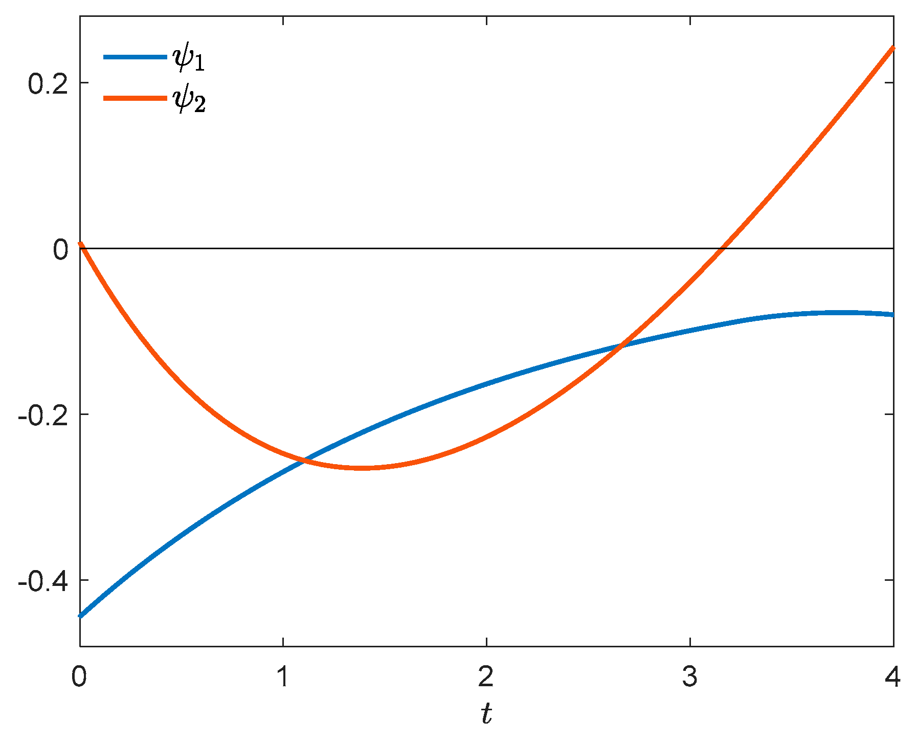
The adjoint function satisfies the final condition . The state equations in the bound-ary intervals are obtained by the substitution in (27), which gives
Hence the pre-Hamiltonian and the adjoint equations in the boundary intervals read
At every entry point the jump condition (13) is valid with the matrix (24), whence , , . We further compute
and from (25), for every . Note that is always positive, and and have the same sign.
Assume that the control u is optimal. It follows from Corollary 2 that for every t in any nonboundary interval of u
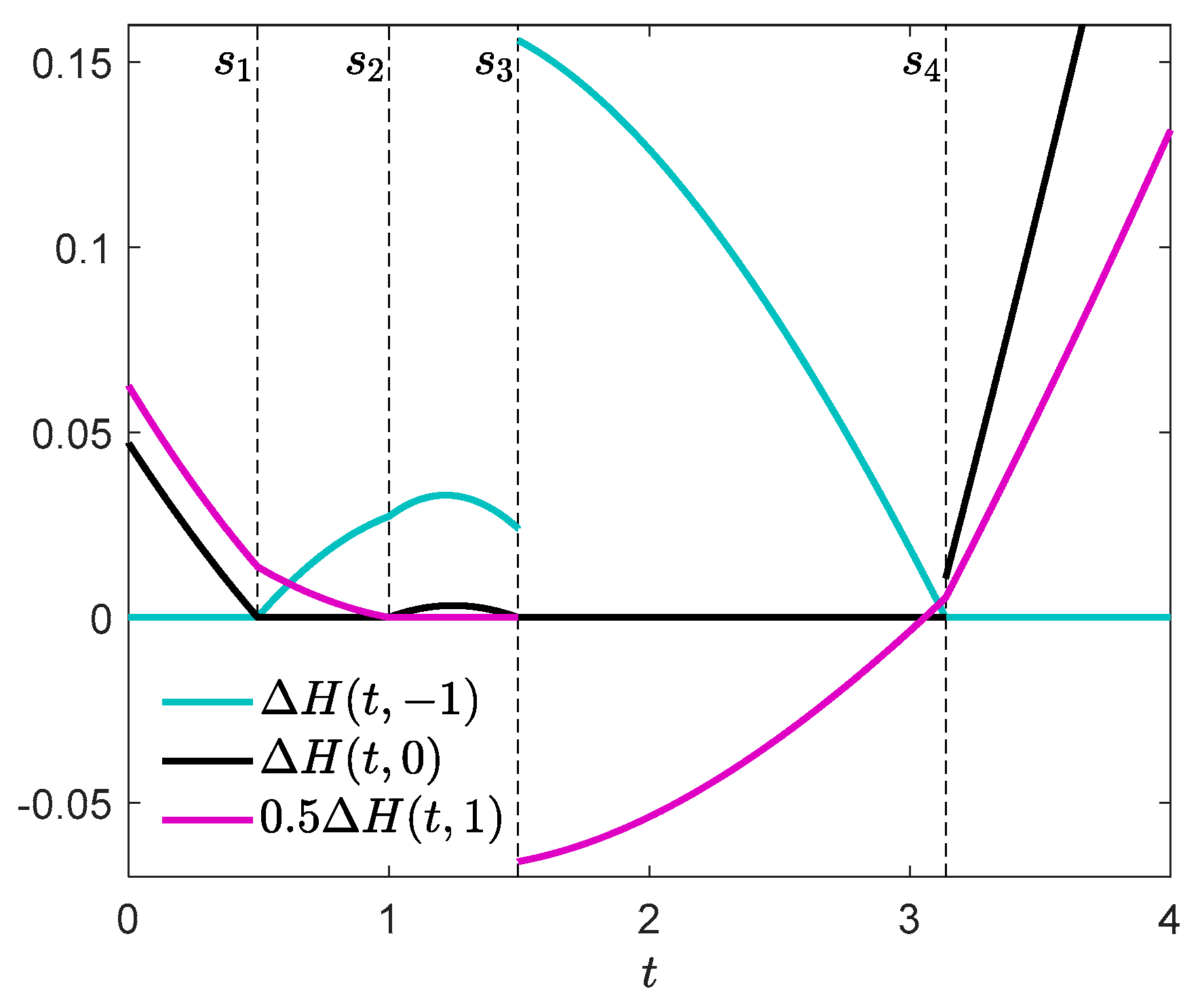
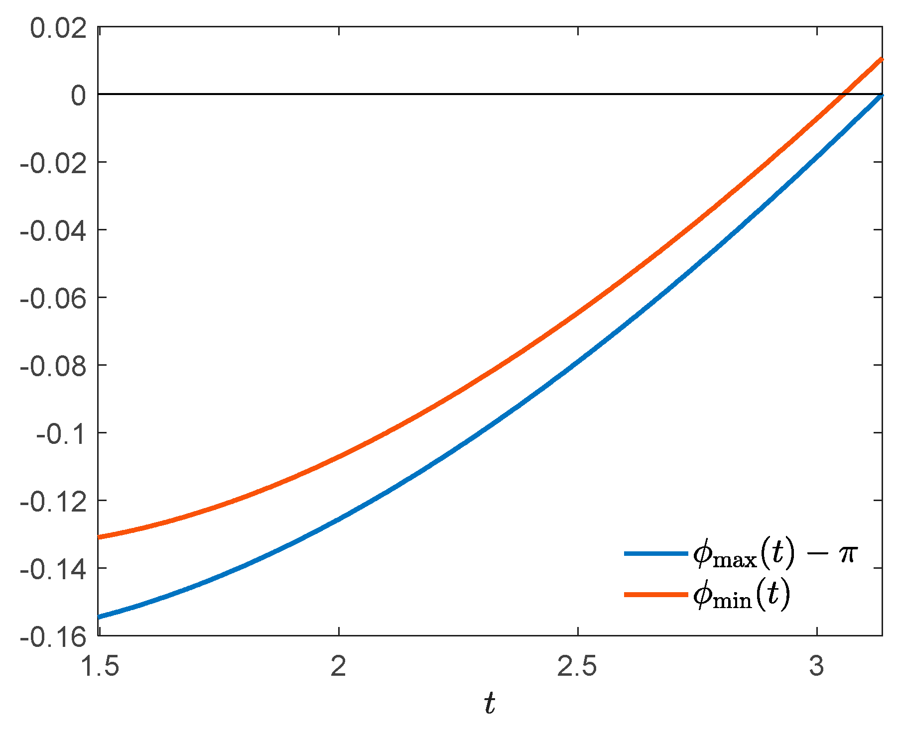
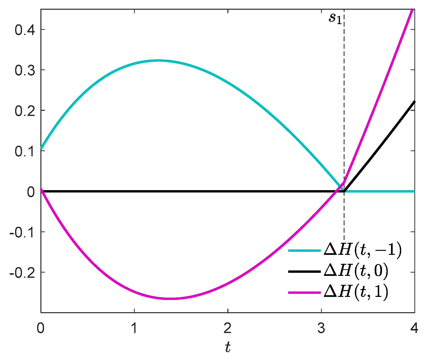
Let now be a boundary interval of u. We infer from Corollary 2 that if , then or . If these relations are not satisfied at some , then the control u can be improved in accordance with Lemma 5, by means of a spike control variation described in Section 2. We deduce from Theorem 5 that if , , and , then
- (i)
- if and ,
- (ii)
- if and ,
- (iii)
- if and .
If some of the necessary conditions of Theorem 5 or Corollary 4 are not fulfilled, then—as follows from Lemma 6—the control u can be improved with the use of a two-spike control variation (Section 4).
We shall now numerically analyze two cases, taking , , , , and .
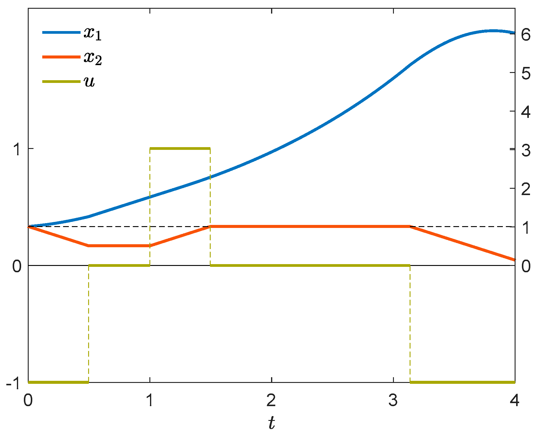
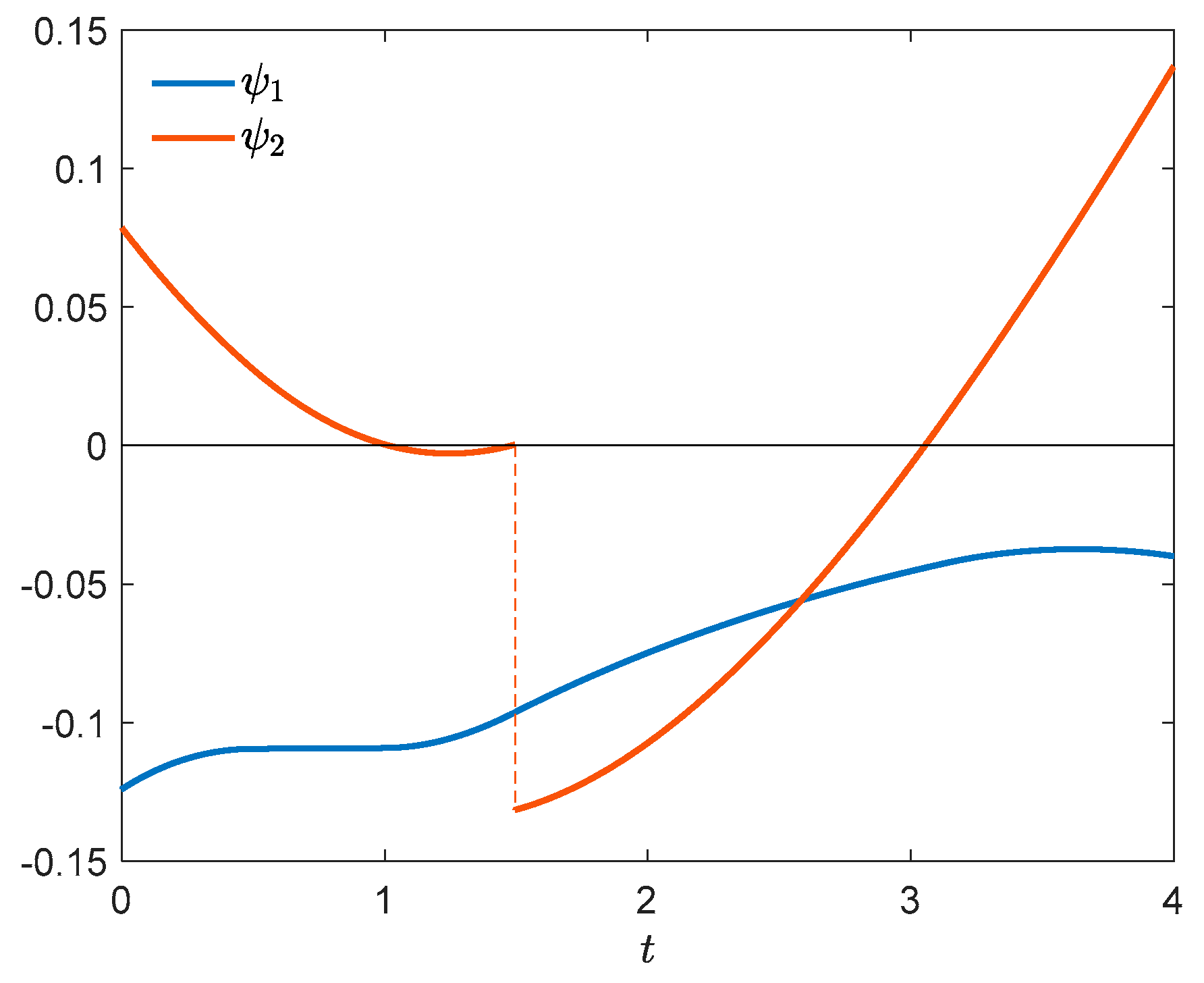
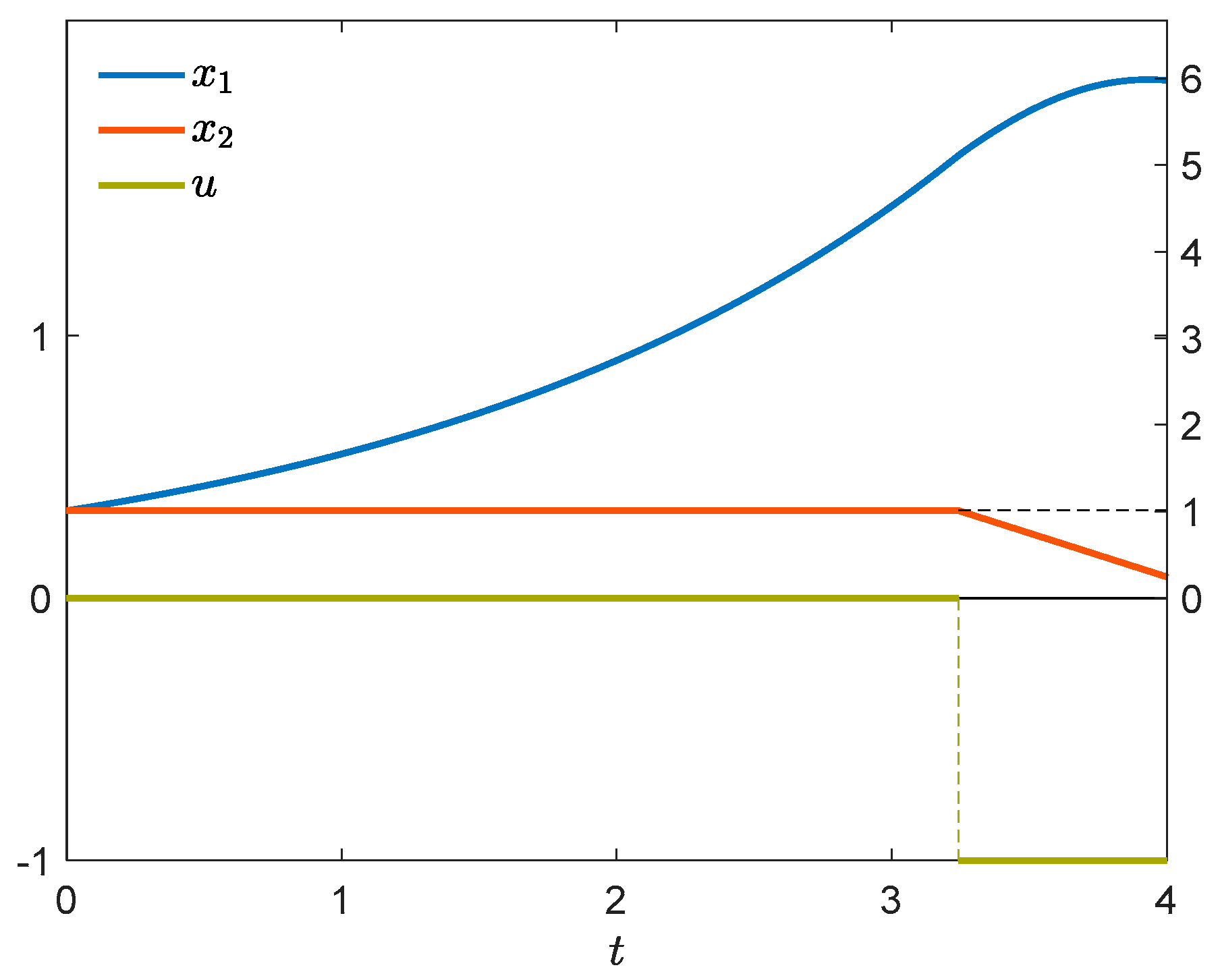
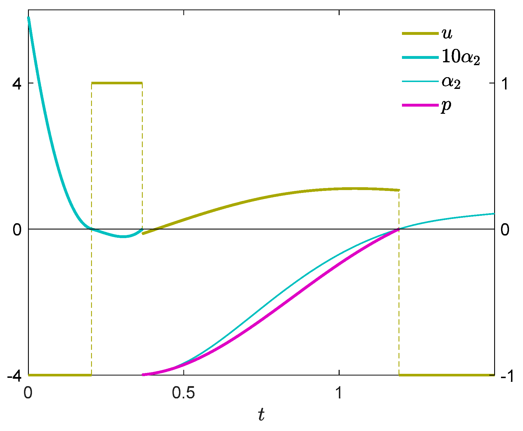
Example 2a.
The optimal control in the considered problem is of the form
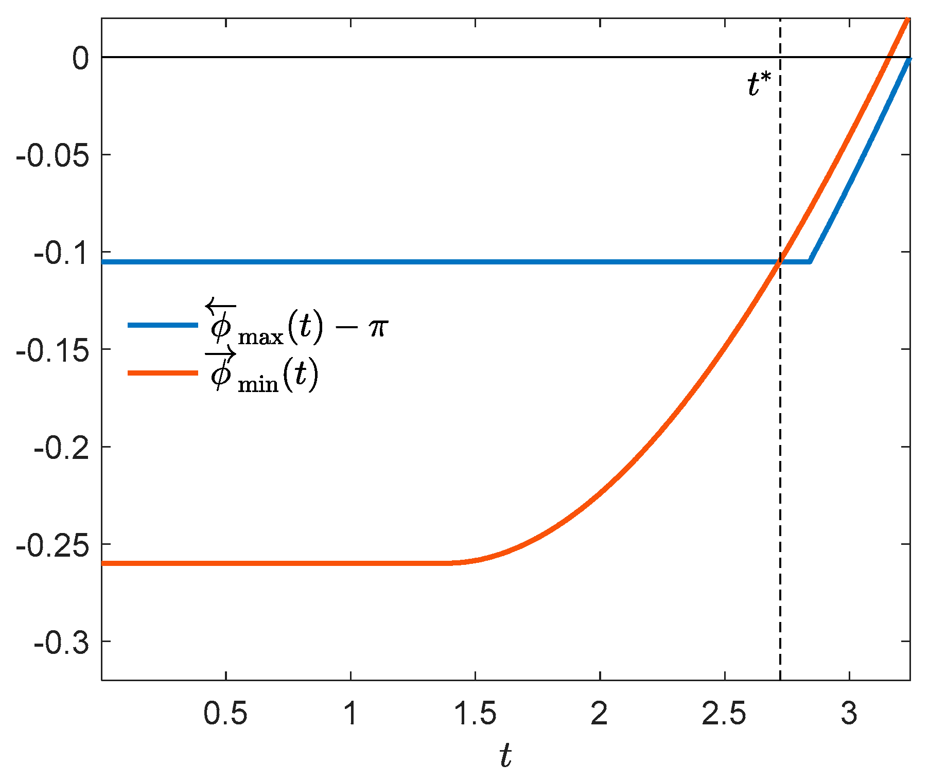
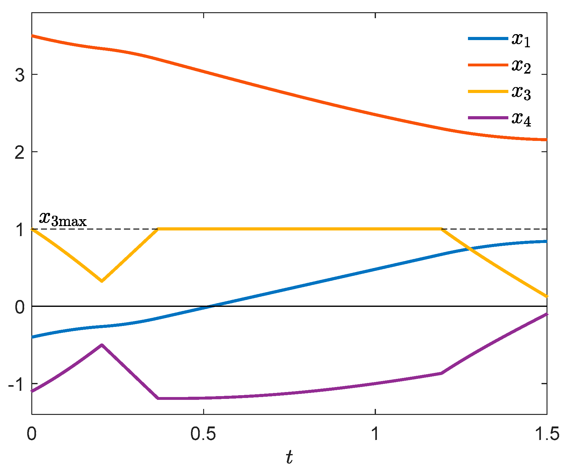
where , , , with . Figure 9 shows the control u, the switching function , and the function p (25). It is easy to see that the necessary optimality conditions of Theorems 4 and 5 are fulfilled in the whole interval . The optimal state trajectory is depicted in Figure 10. Notice the cusps of at and , indicating that u satisfies the nontangentiality conditions and is verifiable.
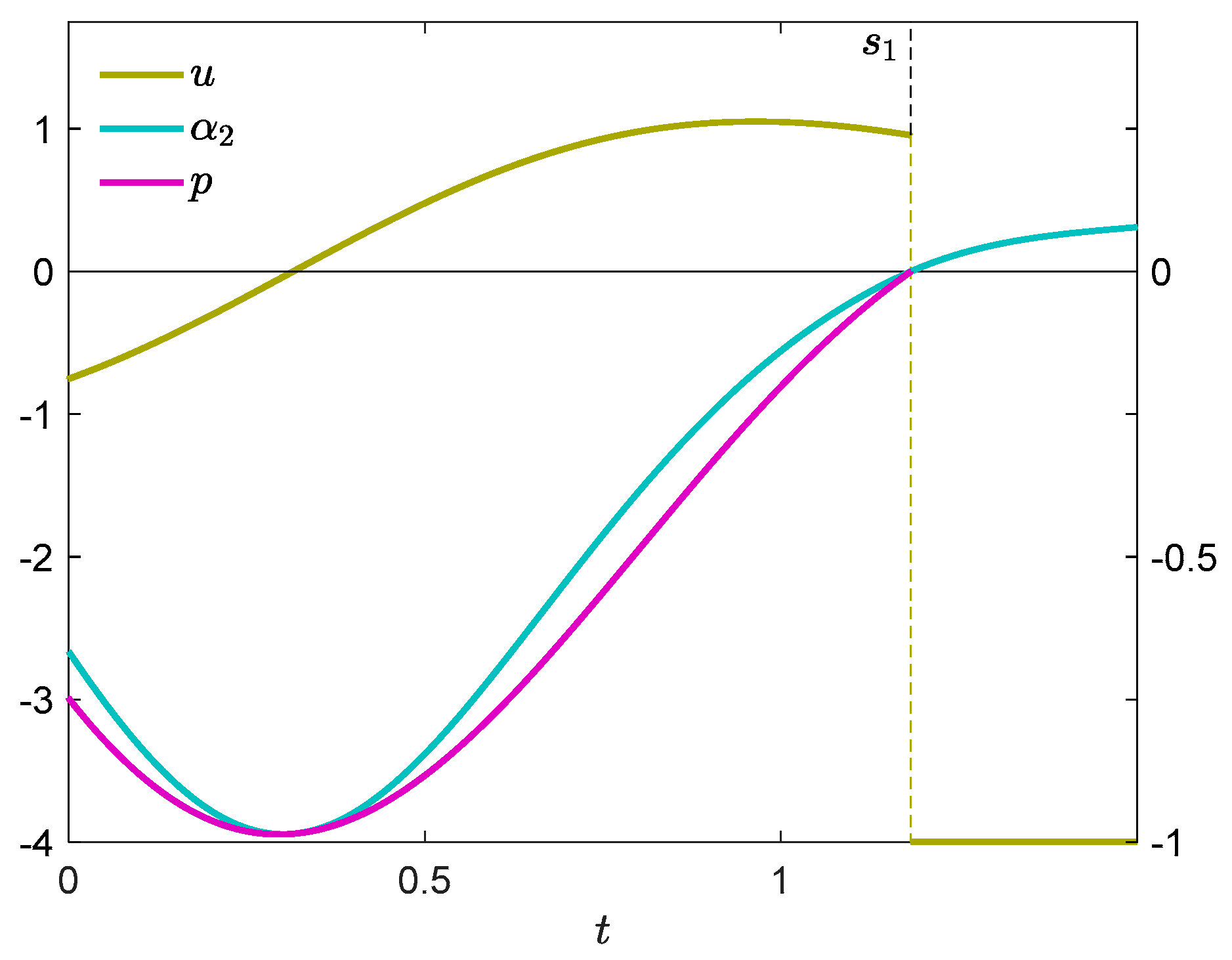
Example 2b.
Consider a verifiable, but nonoptimal control with a boundary interval
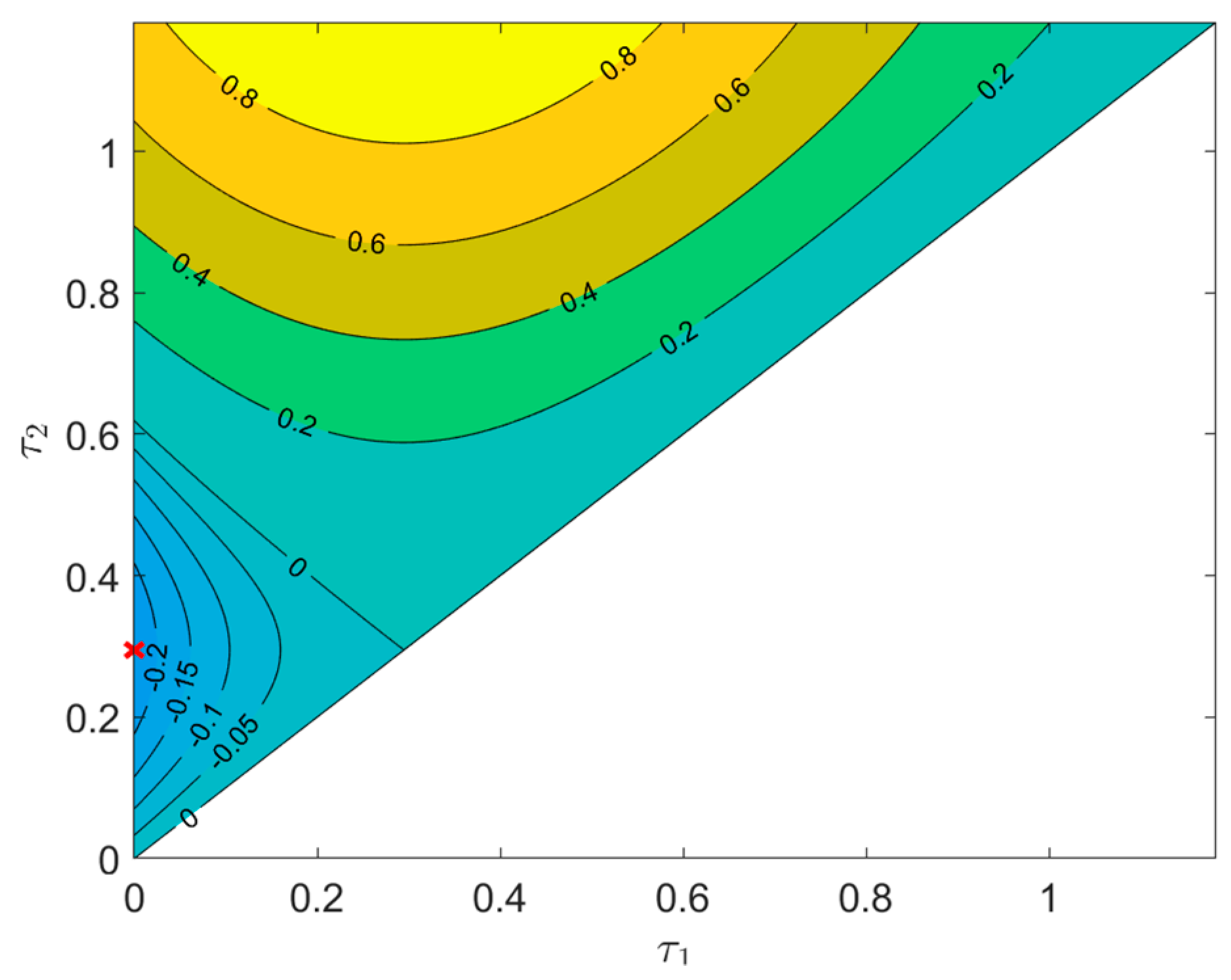
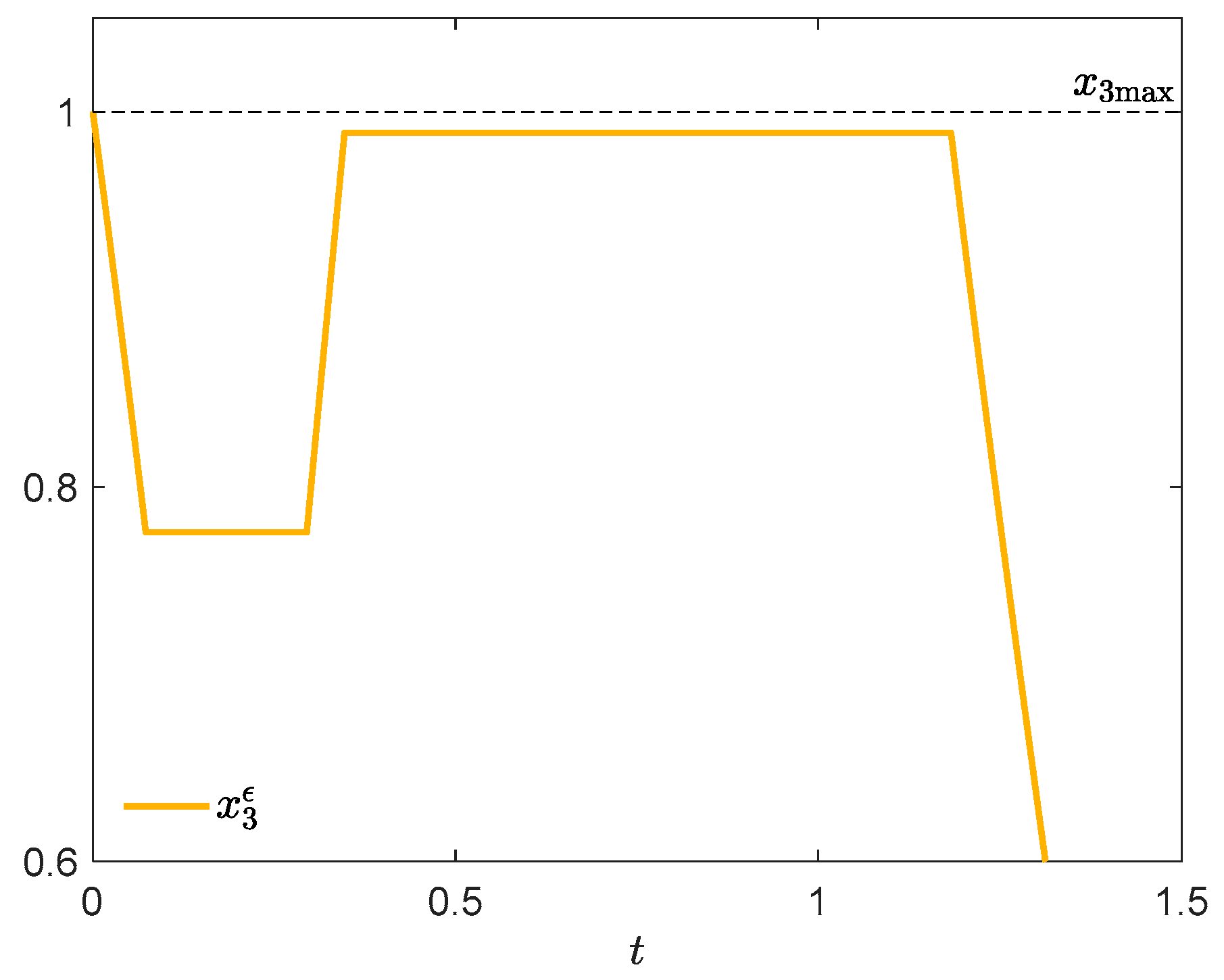
The corresponding value of cost is . Figure 11 presents the control u, the switching function , and the function p (25). It can be seen that the necessary conditions of Theorem 4 and Corollary 2 are satisfied, which means that there are no one-spike control variations described in Section 2, guaranteeing an improvement of the cost. Figure 12 shows the state trajectory. The plot of has a cusp at the exit point , and so the control u is verifiable. We can also see in Figure 11 that in the time interval [0, 0.2948] the function p is decreasing, hence it is possible to construct a two-spike control variation in that interval (according to Section 4) which reduces the cost. In order to verify this numerically, consider also Figure 13 which presents a contour plot of the difference . Let for instance , , , (red cross on the left y-axis). By (26), the parameter may have an arbitrary value from the interval ; we choose . Figure 14 demonstrates the dependence of the cost increment on the width of the first spike . The greatest improvement takes place at . For , Figure 15 shows the state trajectory, and Figure 16, an enlargement of the plot of .
9. Connections with Some Classical Results
There are essential connections between some of our results presented in Section 5 and Section 7, and certain classical results obtained by the so called indirect adjoining method, dating back to the works of R.V. Gamkrelidze, A.E. Bryson, H. Maurer, D.H. Jacobson, and many others (see [1,3,4,5]). As we have no space to discuss all similarities and analogies that can be found in the vast literature, we shall concentrate on one representative theorem due to H. Maurer [3]. We shall use a reduced version of that theorem, specialized to the case of state constraint of order one, verifiable control, fixed initial state and free final state.
Consider the optimal control problem formulated in Section 1, with the additional assumption that U is a closed interval with nonempty interior. Define
Theorem 6 ([3], Theorem 5.1).
Let u be a verifiable optimal control and x, the corre-sponding state trajectory. Suppose that f and g are of class, and letandfor every t in any boundary interval. Additionally, assume that there are finitely many entry points. Then there exist a numberand functions,such that
The following jump condition holds
at every entry point, andis continuous at every exit point.The functionsatisfiesonand is afunction in the interiorof every boundary interval, given by
Moreover,andfor. It also holds that for a.e.
Let us first notice that if in (31) is identical with the adjoint , then the multiplier is equal to the function given by (22) in Section 5. The function , similarly to , is nonnegative and nonincreasing in every boundary interval. The adjoint Equation (28) is then identical with (11) almost everywhere. Indeed, in every boundary interval the Equation (11) takes the form
By virtue of Section 1 and (22),
Hence if , then . The final condition (29) coin-cides with (12) if . This last equality is ensured in [3] by special regularity conditions. Further, it is evident that the jump condition (13) can be written in the form
Thus, in this case (30) is identical with (13) if
In the control affine case discussed in Section 7 the condition (13) is readily transformed to
with p determined by (25). Hence, we have by Corollary 4. We skip the proof of the inequality sign in the general case, which is more complicated. The identity of the adjoints and entails the equivalence between the minimum conditions (32) and (23). In conclusion, the results obtained in this work for the case where in the boundary intervals , and is given by (22) or (25), are in agreement with Theorem 5.1 in [3].
Finally, note that this work’s approach does not require that the optimal control in the boundary intervals takes values in the interior of U, whereas that assumption is essential in [3]. Also, in contrast to [3], we give an explicit representation of the jump of the adjoint function (Section 3, see also [11,12]).
Author Contributions
Conceptualization, methodology, investigation, writing—A.K. and M.S. All authors have read and agreed to the published version of the manuscript.
Funding
This research received no external funding.
Institutional Review Board Statement
Not applicable.
Informed Consent Statement
Not applicable.
Data Availability Statement
Data sharing not applicable.
Acknowledgments
The authors thank the two anonymous reviewers for their comments that helped to improve the paper.
Conflicts of Interest
The authors declare no conflict of interest.
References
- Pontryagin, L.S.; Boltyanskii, V.G.; Gamkrelidze, R.V.; Mishchenko, E.F. The Mathematical Theory of Optimal Processes; Nauka: Moscow, Russia, 1961; (in Russian, first English language edition: Wiley & Sons, Inc., New York, 1962). [Google Scholar]
- Karamzin, D.; Pereira, F.L. On a Few Questions Regarding the Study of State-Constrained Problems in Optimal Control. J. Optimiz. Theory App. 2019, 180, 235–255. [Google Scholar] [CrossRef]
- Maurer, H. On the Minimum Principle for Optimal Control Problems with State Constraints; Universität Münster: Münster, Germany, 1979. [Google Scholar]
- Hartl, R.F.; Sethi, S.P.; Vickson, R.G. A survey of the maximum principles for optimal control problems with state constraints. SIAM Rev. 1995, 37, 181–218. [Google Scholar] [CrossRef]
- Arutyunov, A.V.; Karamzin, D.Y.; Pereira, F.L. The maximum principle for optimal control problems with state constraints by R.V. Gamkrelidze: Revisited. J. Optimiz. Theory Appl. 2011, 149, 474–493. [Google Scholar] [CrossRef]
- Bonnans, J.F. Course on Optimal Control. Part I: The Pontryagin approach (Version of 21 August 2019). Available online: http://www.cmap.polytechnique.fr/~bonnans/notes/oc/ocbook.pdf (accessed on 30 December 2020).
- Bourdin, L. Note on Pontryagin Maximum Principle with Running State Constraints and Smooth Dynamics—Proof based on the Ekeland Variational Principle; University of Limoges: Limoges, France, 2016; Available online: https://arxiv.org/pdf/1604.04051v1.pdf (accessed on 30 December 2020).
- Dmitruk, A.; Samylovskiy, I. On the relation between two approaches to necessary optimality conditions in problems with state constraints. J. Optimiz. Theory Appl. 2017, 173, 391–420. [Google Scholar] [CrossRef]
- Vinter, R. Optimal Control; Birkhäuser: Boston, MA, USA, 2000. [Google Scholar]
- Korytowski, A.; Szymkat, M. On convergence of the Monotone Structural Evolution. Control Cybern. 2016, 45, 483–512. [Google Scholar]
- Bonnans, J.F. The shooting approach to optimal control problems. IFAC Proc. Vol. 2013, 46, 281–292. [Google Scholar] [CrossRef] [Green Version]
- Bonnans, J.F.; Hermant, A. Well-posedness of the shooting algorithm for state constrained optimal control problems with a single constraint and control. SIAM J. Control Optim. 2007, 46, 1398–1430. [Google Scholar] [CrossRef] [Green Version]
- Chertovskih, R.; Karamzin, D.; Khalil, N.T.; Pereira, F.L. Regular path-constrained time-optimal control problems in three-dimensional flow fields. Eur. J. Control 2020, 56, 98–106. [Google Scholar] [CrossRef] [Green Version]
- Cortez, K.; de Pinho, M.R.; Matos, A. Necessary conditions for a class of optimal multiprocess with state constraints. Int. J. Robust Nonlinear Control 2020, 30, 6021–6041. [Google Scholar] [CrossRef]
| 1 | PC(0,T; U) is the space of all functions [0,T] → U which have a finite number of discontinuities, are right-continuous in [0,T[, left-continuous at T, and have a finite left-hand limit at every point. |
| 2 | Controls leading to state trajectories with boundary touch points are not verifiable. |
Figure 1.
Optimal control (left scale) and optimal state trajectory (right scale).

Figure 2.
Adjoint trajectory.

Figure 3.
Verifying conditions of Theorems 1 and 2.

Figure 4.
Verifying the conditions of Theorem 3.

Figure 5.
Control (left scale) and state trajectory (right scale).

Figure 6.
Adjoint trajectory.

Figure 7.
Verifying the condition of Theorem 1(i).

Figure 8.
Verifying the conditions of Theorem 3.

Figure 9.
Optimal control (left scale), switching function and p (right scale).

Figure 10.
Optimal state trajectory.

Figure 11.
Control (left scale), switching function and p (right scale).

Figure 12.
State trajectory.
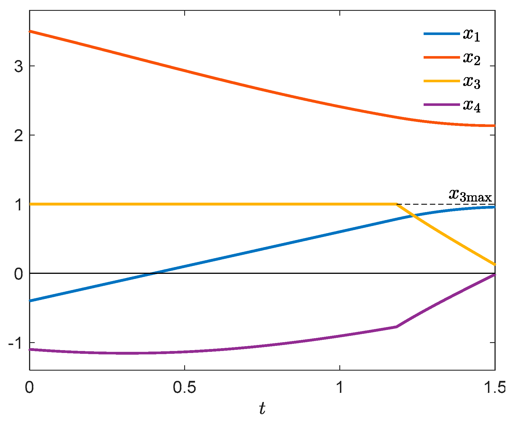
Figure 13.
Contour plot of .

Figure 14.
Cost increment vs. width of first spike.
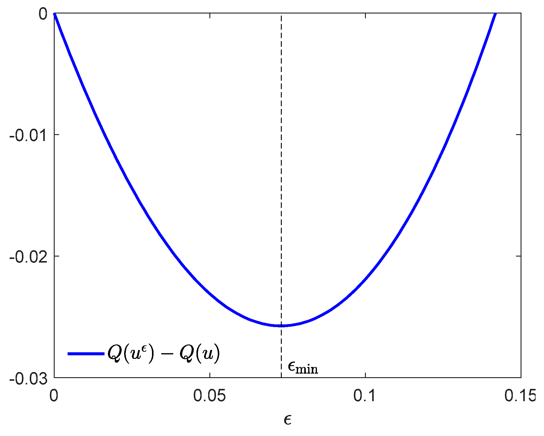
Figure 15.
State trajectory .
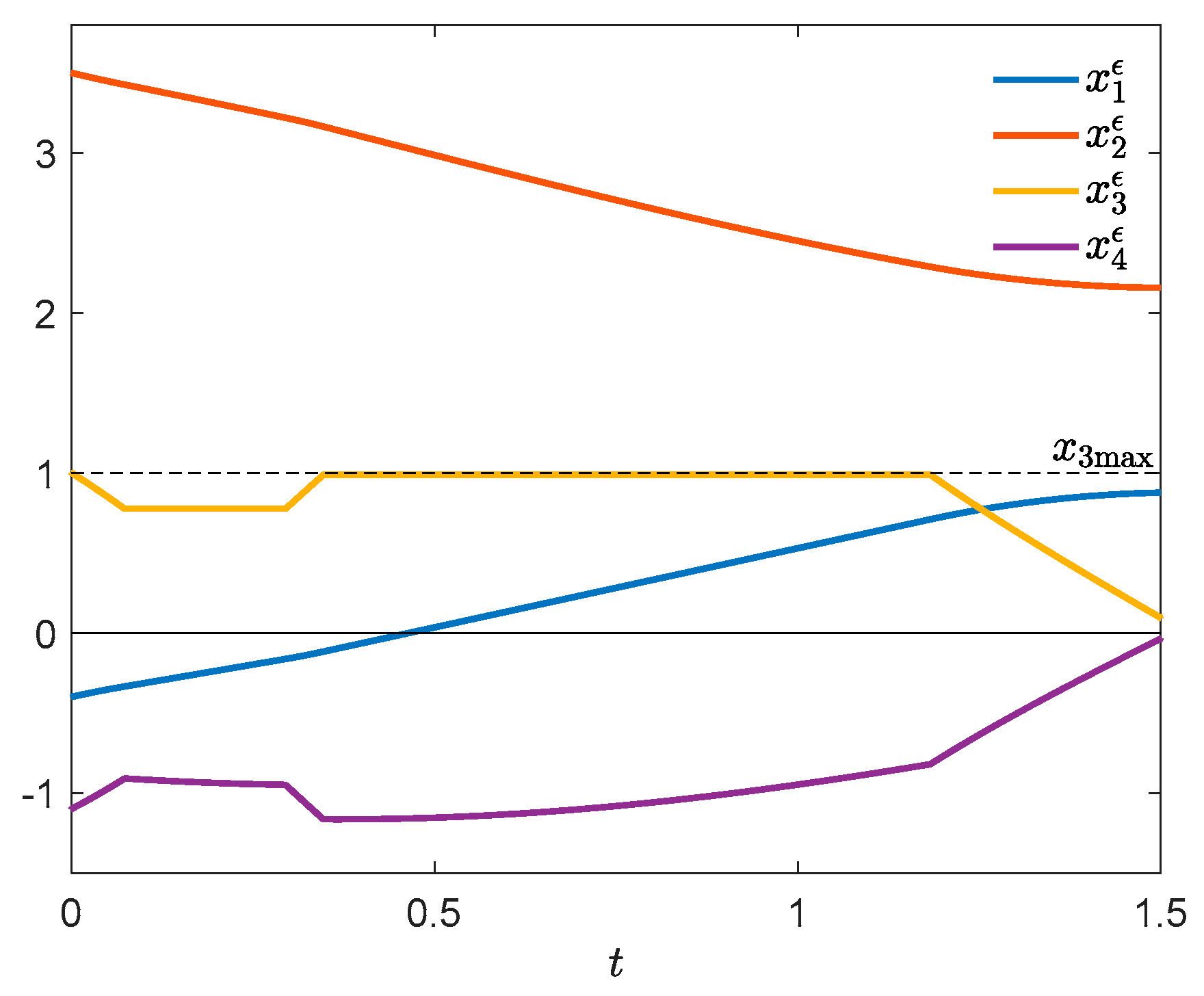
Figure 16.
Blow-up of .
Publisher’s Note: MDPI stays neutral with regard to jurisdictional claims in published maps and institutional affiliations. |
© 2021 by the authors. Licensee MDPI, Basel, Switzerland. This article is an open access article distributed under the terms and conditions of the Creative Commons Attribution (CC BY) license (http://creativecommons.org/licenses/by/4.0/).
Share and Cite
MDPI and ACS Style
Korytowski, A.; Szymkat, M. Necessary Optimality Conditions for a Class of Control Problems with State Constraint. Games 2021, 12, 9. https://0-doi-org.brum.beds.ac.uk/10.3390/g12010009
AMA Style
Korytowski A, Szymkat M. Necessary Optimality Conditions for a Class of Control Problems with State Constraint. Games. 2021; 12(1):9. https://0-doi-org.brum.beds.ac.uk/10.3390/g12010009
Chicago/Turabian StyleKorytowski, Adam, and Maciej Szymkat. 2021. "Necessary Optimality Conditions for a Class of Control Problems with State Constraint" Games 12, no. 1: 9. https://0-doi-org.brum.beds.ac.uk/10.3390/g12010009
Note that from the first issue of 2016, this journal uses article numbers instead of page numbers. See further details here.