
A Double-Weighted Bankruptcy Method to Allocate CO2 Emissions Permits

1
LAMSADE, CNRS, Université Paris-Dauphine, Université PSL, 75016 Paris, France
2
LARODEC, Institut Superieur de Gestion de Tunis, University of Tunis, Tunis 2000, Tunisia
*
Author to whom correspondence should be addressed.
Games 2021, 12(4), 78; https://0-doi-org.brum.beds.ac.uk/10.3390/g12040078
Submission received: 6 September 2021
/
Revised: 12 October 2021
/
Accepted: 14 October 2021
/
Published: 23 October 2021
(This article belongs to the Section Applied Game Theory)
Abstract
:Global warming, as a result of greenhouse gases, is exceeding the planet’s temperature stabilization capacities. Thus, greenhouse gas emissions must be reduced. We analyse a bankruptcy situation aimed at allocating emissions permits of CO2, the predominant greenhouse gas emitted by human activities. Inspired by the Constrained Equal Awards (CEA) solution for bankruptcy situations, we introduce a new allocation protocol based on the extension of the CEA solution over double-weighted bankruptcy situations, including two exogenous parameters aimed at providing a balance, in the request of emissions permits, between economic activities and the production of renewable energy. In these bi-criteria allocation problems, we focus on a computational approach to find an allocation protocol that does not prioritize any particular parameter. As an application of our method, we first consider CO2 permit allocation problems in European Union (EU) countries, using real data about the gross domestic product (GDP), the production rate of renewable energies, and countries’ ‘demands’ of CO2 emissions from 2010 to 2014. Then, we compare our approach with the CEA solution and its single-weighted extension to show the impact of using two weights over the distribution of CO2 emissions permits; we analyse the correlation between allocations of CO2 emission permits and the distribution of power within the EU Council to study the acceptability of alternative allocations.
1. Introduction
Climate change and global warming is a major challenge for the international community. Greenhouse gases, in particular carbon dioxide (CO2), accumulated in the atmosphere, cause irreversible damages, and the time required for their repairs could last hundreds of years. Emissions must be reduced by moving to clean and renewable energy resources, and the study of responsible sharing policies, in particular CO2 emissions, is one of the main goals of international climate policies nowadays. The literature on international cooperation on climate change has been organized around various international cooperation forms [1]. The existing methods proposed for emission allowances in CO2 can be classified into four groups: indicator approach based on one or more indicators, optimization approach, game theory approach, and hybrid approaches [2]. Certain allocation criteria are based upon equity principles, such as the grandfathering, consisting of giving an equal right to emit for all countries, the egalitarianism, giving to each person the same right to emit, or historical responsibility, according to which long-standing polluters should face a greater reduction rate, or other principles of distributive justice [3]. Other allocation criteria, where countries are compensated for reducing their emissions, follow a principle of efficiency, such as the approach proposed in [4], where the authors argue that efficiency can be defined as a type of “fairness”. In practice, alternative methods have been proposed to allocate CO2 emissions among countries and taking into account criteria, such as energy, the gross domestic product (GDP), population, energy production, etc. (see [2], for a recent survey), but no consensus has been reached on any particular allocation protocol.
However, the increasing amount of gas emissions and the limited absorption rate of the planet, on the one hand1, and the fact that countries, in 2020, have already consumed in 8 months2, all the resources that ecosystems can produce in a single year, it is obvious that we are facing a claims problem [5,6]. Claims problems, also called bankruptcy situations, are situations where a given quantity of a divisible resource must be allocated among a group of agents. Each agent has his own demand, and the total amount of divisible resources cannot satisfy the demand of all agents. Thus, the problem is to formulate a fair allocation rule or solution [7] (for a survey on bankruptcy situations, solutions, and their properties see, for instance, [8,9]). Bankruptcy situations can model different real ecological problems where a scarce resource, such as food, fishing quotas, medical suppliers, carbon budget, or water has to be shared among countries, or among the individuals of a population [10].
In this paper, we focus on the allocation of the most important greenhouse gas, carbon dioxide, whose emissions permits must be shared among European Union (EU) countries, and where each country has its own claim of CO2 emissions permits. This is not the first time that bankruptcy situations have been applied to study this problem at the EU level. For instance, two bankruptcy allocation solutions from the literature, namely, the Constrained Equal Awards (CEA) [7,8,11] and the Weighted Constrained Equal Awards (WCEA) [12,13], have been used in [14] to allocate CO2 emissions permits using EU countries’ CO2 claims and an exogenous weight based on the GDP. For other applications of bankruptcy situations to the allocation of emissions permits, see also [6]. As far as we know, however, this is the first study where the CO2 allocation problem has been investigated as a claims problem from a multi-criteria point of view. Specifically, in this paper, we introduce a preliminary application of a new allocation method for double-weighted bankruptcy situations based on the combination of two distinct criteria: the ability of countries to efficiently use their CO2 emissions permits, and the capacity of countries to produce energy in a sustainable manner via renewable sources. More precisely, using an extended version of the CEA solution for bankruptcy situations, we leverage the request of CO2 emissions permits of EU countries, taking into account both the economic growth of EU countries (in terms of their GDP) and their sustainable policies, measured as the amount of renewable energy produced by each country. We also compare the allocation of CO2 emissions permits provided by the methods considered in this paper with the distribution of power among the members of the EU Council, which is the main decision making body in the EU. As a main result of our analysis, we show that the double-weighted allocation protocol well represents the effective power of countries within the EU Council, and for this reason it could benefit from a more general consensus within the EU.
The remainder of the paper is organized as follows. The next section is devoted to the introduction of bankruptcy situations, and to the presentation of related basic notions and notation. Then, Section 3 introduces a new family of bi-criteria allocation methods for double-weighted bankruptcy situations, namely, the Double-Weighted Constrained Equal Awards (DWCEA) methods, and presents an algorithm to compute a specific allocation protocol. Section 4 is devoted to the application of the proposed protocol introduced in Section 3 to allocate CO2 emissions permits among EU countries over the years 2010–2014, and to the comparison of the results provided by the alternative solutions considered in this study. Section 5 concludes.
2. Preliminary
A bankruptcy situation or bankruptcy problem occurs when there is an infinitely divisible resource, the estate, to be divided among several agents having different claims and the same preferences, but there are natural upper limits on the allocation: none should be awarded more than his demand. Formally, a bankruptcy situation [15], or a claims problem, is defined by a tuple (or, simply, if the set N is already clearly identified), where is a set of agents, the estate is such that , and is a vector of agents’ claims. So, the problem is to divide E among the agents of N, each agent having her/his own claim .
To allocate the estate E among the agents in N, we define an allocations vector as a real valued vector , respecting the following properties:
- rationality: , for all ;
- claim boundedness: , for all ;
- efficiency: .
So, according to an allocation vector, every agent should receive a non-negative allocation, smaller or equal than her/his claim, and the entire estate should be divided completely among the agents. We are interested in defining a general allocation method, also called rule or solution, which is a function that associates to each bankruptcy situation an allocation vector. In the literature on bankruptcy situations, several rules have been proposed to allocate the estate (see, for instance, [7,8,9,11]).
In this work, we will focus on the Constrained Equal Awards (CEA) rule, and on some weighted version of the CEA rule. Formally, for each bankruptcy situation with N as the set of players, the rule yields an allocation vector , such that:
for each agent and where and
This method can be defined as an iterative procedure. In the first iteration, all agents receive the same amount of estate, which must be smaller or equal than the smallest claim among the agents. Then, the agents with the smallest claim leave the game. A new iteration starts by equally allocating the remaining part of the estate, if any, among the remaining agents, and paying attention to allocate to each agent no more than the second smallest claim. Then, the agents claiming the second smallest claim leave the game, and the procedure is repeated among the remaining agents until there is no more estate to be shared.
A weighted bankruptcy situation [12,13], is a triple where is a bankruptcy situation and is a vector of positive weights. The Weighted Constrained Equal Awards (WCEA) solution [12,13] is inspired by the CEA rule, and takes into account not only players’ claims, but also their weights, which modify the impact of the claims over the final allocation. The allocation vector provided by the WCEA rule is the unique vector such that:
for each agent and where the parameter is such that
In the last section of this paper, we also make use of some concepts from cooperative game theory. Specifically, we compare allocation vectors for bankruptcy situations with the vector provided by the Shapley and Shubik (Sh–Sh) power index [16] for a simple game representing the voting rule at the EU Council [17]. A simple game is a pair where N is a set of agents, or voters, and v is the characteristic function of the game that associates to each coalition a value such that and . The standard interpretation of a simple game is that means that coalition S is winning, according to some voting rule, while means that S is losing, according to the same voting rule. The Shapley and Shubik power index [16] is defined as the map associating to any simple game a vector of numbers representing the P-power of voters [18], which is interpreted as the voters expected shares of a fixed prize for winning the elections, and is computed as the expected marginal contribution of each voter over all possible permutations of voters, i.e., , where s is the cardinality of coalition S.
3. Double-Weighted Constrained Equal Awards Rule (DWCEA)
Previous studies on bankruptcy situations and their solutions can be seen as an allocation approach where only one criterion, agent’s claim, is considered. Weighted bankruptcy situations [12] keep into account one more parameter to determine allocation vectors. In this section, we introduce a richer framework for bankruptcy situations, considering two vectors of weights at once, in addition to the vector of claims.
We denote by a double-weighted bankruptcy situation on a set of agents N and where is a strictly positive estate, is the vector of non-negative claims such that , and and are two vectors of non-negative weights. We denote by the family of all double-weighted bankruptcy problems. An allocation rule is a map that associates to any double-weighted bankruptcy situation an allocation vector in such that . Some interesting properties for an allocation rule for double-weighted bankruptcy situations are the following. Equal treatment: an allocation rule satisfies equal treatment if for all , if are such that , and , then . Composition: An allocation rule satisfies composition if for all such that for all and for all we have Invariance under claims truncation: an allocation rule satisfies invariance under claims truncation if for all we have , where is such that for all .
In the attempt to further extend the WCEA rule to situations with two vectors of weights, in this paper, we introduce a Double-Weighted Constrained Equal Awards (DWCEA) solution, which associates to any double-weighted bankruptcy situation a particular allocation vector satisfying the following conditions:
for each agent and with such that
As it often happens in multi-criteria decision problems, in general, we face a wide choice of allocation vectors that satisfy the constraints specified by relations (5) and (6) for some and . Therefore, in order to select a specific allocation vector, in the next section we introduce a computational approach to find parameters and that do not require to assume any specific priority on the criteria represented by the two weight vectors.
A DWCEA Solution Algorithm with No Priority over Criteria
The algorithm studied in this section is based on the general principle that a DWCEA solution should grant the same importance to the different criteria represented by the two weight vectors. Based on this assumption, we introduce Algorithm 1 providing a solution for problem (5) under the constraint (6) with the objective to find feasible and without arbitrarily promoting the use of one of the two criteria to drive the choice of these parameters.
| Algorithm 1. Double-Weighted method’s algorithm |
Input: Estate E, Set of player N, Claims vector c, weight vectors , Output: an allocation vector ForEach : , , , ForEach : Begin Bloc 1: if then ForEach : end if End Bloc 1 while AND do if then Algorithm A1 end if if then Algorithm A2 end if end while return x |
Algorithm 1 starts by calculating, for every player , a value and a value , then it sorts these values in incremental order, yielding vectors and . In the initial iteration, the same value is affected to parameters and , which are the temporary parameters used to compute the allocation. Starting the search for parameters and from the median ensures a kind of neutrality for the importance of both criteria in the allocation computation, and it guarantees a minimal worst-case number of iterations before reaching the final and , since this procedure will be iterated at most times. At each iteration of the algorithm, the sum of the allocations, , can take three possible values:
- (1)
- , i.e., the sum of allocations is equal to the estate. In this case, we immediately have that and .
- (2)
- , i.e., the sum of allocations is strictly larger than the estate. So, and/or must be decreased. In this situation, Algorithm 1 selects the first sorted as X and the first sorted as Y. Then, we choose the biggest value among X and Y to change the corresponding value, , and we keep the same value for the other ; then, we recompute S and we reiterate the procedure until we obtain , as shown in Algorithm A1 (see Appendix A).
- (3)
- , i.e., the sum of allocations is strictly smaller than the estate, we have to increase and/or . So, , , will be updated to the smallest value among X, the first , and Y, the first , and we keep the same value for the other ; then, we recompute S and we re-iterate the procedure until we obtain , as shown in Algorithm A2 (see Appendix A).
After a number of iterations , half of the agents’ demands are considered, and if the sum of allocations does not satisfy the efficiency constraint, , the algorithm starts the “LastComputing” procedure. The same “LastComputing” procedure is also called at an iteration such that and such that at iteration (or, inversely, at iteration such that and such that at iteration ). Basically, as shown in the corresponding pseudo-code in Appendix A, the Last “LastComputing” procedure transforms the double-weighted bankruptcy situation with two weight vectors in a single weighted bankruptcy situation, using the parameter , , which did not change since the previous iteration.
It is obvious that the solution provided by Algorithm 1 satisfies the equal treatment property. It also satisfies the composition property, as any solution satisfying conditions (5) and (6) when applied to a double-weighted bankruptcy problem with yields the allocation provided by the WCEA solution applied to the weighted bankruptcy problem , and the WCEA solution satisfies the composition property on the class of weighted bankruptcy problems (see [12,13]). Instead, we cannot guarantee that the solution provided by Algorithm 1 satisfies the property of invariance under claims truncation, as the use of vector instead of c may affect the procedure to compute and along the iterations of Algorithm 1.
We now introduce an example of calculations provided by Algorithm 1.
Example 1.
Consider the double-weighted bankruptcy situations with as the set of agents, and the other parameters as shown in Table 1.
At the first iteration of Algorithm 1, the vectors and are defined to sort the ratios and , respectively, and the value is calculated as the average of the two medians of and . This value is assigned to the variables and . The provisional allocation for the three agents is computed as for agent 1, for agent 2 and for agent 3. For the sum of allocations is larger than the estate , the procedure calls Algorithm A1 (see Appendix A). Now, at the new iteration ( in Table 2), the procedure selects the largest value between and which is also smaller than , and such a value is used to set the new for the corresponding weight , while the value is maintained equal to its value at the previous iteration. So, at , and . A new allocation for and is computed, and the procedure continues as detailed in in Table 2, till the sum of allocations becomes strictly smaller than the estate (this happens at the iteration of Table 2. At this point, the largest (and closest to ) value between the and is selected (so, in the specific case), and the process is called to calculate the final allocation corresponding to the WCEA allocation defined by relations (3) with claims vector . The relevant parameters calculated at each iteration of Algorithm 1 are shown in Table 2.
Example 2.
Consider the double-weighted bankruptcy situations with as the set of agents, and the other parameters as shown in Table 1. Similar to Example 2, we show all the iterations of Algorithm 1 in Table A1, Appendix B. Notice that at iterations and , it is called Algorithm A2, instead of Algorithm A1, as in Example 1, for at and at .
4. DWCEA Applied to CO2 Emissions Permits
In the context of global climate negotiations, an imperative step is to find an agreement or a strategy to be adopted for the reduction of CO2 emissions. However, CO2 emissions permits are limited and countries have to find a common consensus over methods to allocate emissions permits. In this paper, we analyse EU country claims on CO2 emissions permits, taking into account the limits in emission of CO2 recommended by the Kyoto protocol [19].
In order to retrospectively determine an allocation method that can be considered both efficient and equitable by EU countries, we focus on data provided by the World Bank Open Data project3. Precisely, for each of the five years from 2010 to 2014, we consider a double-weighted bankruptcy situation , , with the 27 EU countries as the set N of agents, and the following features as vectors of claims and weights: the actual CO2 emission data from 2010 to 2014, as the vector of claims ; the quantity of GDP over the same time interval, as the first weight vector reflecting the economic growth rate of a country; finally, the production of renewable energy, as the second weight vector quantifying the sustainability of policies adopted by each country. Figure 1 summarizes the total fraction of these three parameters for the 27 EU countries during the period 2010–2014. According to the Kyoto protocol [19], which imposed by 2010 a reduction of of the CO2 total emissions in 1990, we set the estate E of each of the five bankruptcy problems considered over the years from 2010 to 2014, equal to the of the total amount of CO2 emitted by all EU countries in 1990.
We applied Algorithm 1 to each bankruptcy situation to obtain the DWCEA allocations for years , and we computed the CEA allocations over the bankruptcy situations as well as the WCEA allocations over the weighted bankruptcy problems and , respectively, for each year from 2010 to 2014. All of those allocations of CO2 emissions permits are reported in Table A2, Table A3, Table A4 and Table A5 in Appendix B.
As expected, the allocation yielded by the CEA solution completely satisfies small claims of emission permits. Instead, countries with high demands (i.e., Germany, UK, Italy and France), are drastically limited in their claims and receive the same amount of emission permits. The allocation provided by the WCEA solution based on GDP as the unique weight, favours countries with high GDP by giving more than half of the estate to the four countries with the highest GDP (i.e., Germany, UK, France, and Italy), while using the renewable energy as the unique weight, it completely satisfies some countries with intermediate emissions claims, (e.g., Denmark, Sweden, Finland, and Portugal), as well as countries having high claims and high renewable energy production (e.g., Germany and Spain).
Considering both the GDP and renewable energy as weights in Algorithm 1 to provide a DWCEA method, the countries respecting a specific threshold of both weights receive their total claims of emission permits, as it happens for Denmark, Sweden, Austria, and Spain in 2010, and for France and UK in 2014. Compared to the allocation generated by the WCEA solution based on GDP only as the weight, we can notice that the DWCEA allocation increases the amount of emission permits for 13 countries in 2010, 16 countries in 2011 and 2012, and 19 countries in 2013 and 2014. Instead, compared to the results obtained by the WCEA based on renewable energy as unique weight, we can observe an improvement in allocations for 17 countries for 2010 and 2011, and at least 14 countries from 2012 to 2014. Furthermore, in 2010, Denmark and Sweden were completely satisfied with whatever allocation method is used; Malta and Austria, in 2010, obtained an equal amount by DWCEA and WCEA based on renewable energy only, and Ireland, Finland, and France, in 2014, received the same amount of emissions permits according to DWCEA and WCEA based on GDP only.
We also notice similarities among allocations of some countries over the five studied years. To be more specific, we investigated those similarities by means of an unsupervised clustering technique, namely, the K-means method, based on the 1-distance notion to measure the similarity of each country’s allocation distribution over the years from each cluster’s reference centre [20]. This unsupervised clustering technique aims at grouping records (countries) of the data set into K distinct clusters according to their similarities, and each record can only be found in one cluster at a time. Note that countries’ emissions are naturally divided in small, medium, and high emission levels. For this reason, we applied the K-means method with , to define three distinct groups reflecting the impact on CO2 emissions of different EU countries. The clustering on CO2 emission records over the five years is reported in Table 3(1) and shows a group G1 of countries with low emissions, a group G2 formed by countries with medium emissions and, finally, a group G3 containing high emissions countries.
The results of the clustering procedure using the CO2 emissions and the allocation distributions over the five years provided by the considered solutions CEA, WCEA with GDP only as weight, and WCEA with renewable energy only as weight, and DWCEA are shown in Table 3(2–5), respectively. Table 3(2) shows the clusters in accordance with the allocation distribution over the five years yielded by the CEA solution: notice that countries in groups G1 and G2 have low and medium demands and are totally satisfied with respect to their claims from 2010 to 2014. However, in Group 3, only the Netherlands, which has a medium emission distribution, is totally satisfied over 5 years. Other members of cluster G3 receive the same amount despite their different claims (except Spain, who has been totally satisfied since 2013).
Groups formed according to the allocation distribution over the five years by the WCEA solution based on GDP only, are presented in Table 3(3). We observe that group G1 is defined by countries with a lower GDP, group G2 by countries with intermediate GDP, and the last group, G3, is formed by countries with high GDP. Two countries from group G2 (i.e., Denmark and Sweden), and only one country from group G3 (i.e., France), are totally satisfied throughout the five years. So, these groups show a high association between emissions permits claims and GDP, whose effect plays in favour of countries with a large internal economic production.
In Table 3(4), concerning the clusters on allocation distributions over the five years provided by the WCEA solution based on the renewable energy only over the five years, group G3 contains countries with high emissions, which are also characterized by high levels of renewable energy production. In this group, Spain and Germany obtain their claims for all studied period. Even if the effect of the activities producing CO2 is still predominant, here, countries with a high production of renewable energy show a similar allocation distribution over time, and those that are fully satisfied for at least three years are in groups with intermediate and high claims and also high renewable energy production at the same time.
Finally, Table 3(5) presents the clusters generated on the allocation distribution over the years by the DWCEA allocation method. In this case, clusters are more homogeneous because they are generated by a balance among their claims, their economic levels, and their attitudes to employ green energy. According to the DWCEA allocation distribution over time, only Ireland, Denmark, Sweden, and Austria receive their full claims for at least three years due to their weight on renewable energy production. So, the trade-off between GDP and renewable energy production in the DWCEA allocation method seems to play in favour of countries characterized by intermediate levels of CO2 claims and GDP and, at the same time, good levels of renewable energy production.
The clusters provided by the K-means analysis can be interpreted as groups of countries equally affected by each proposed allocation method over the years. So, it seems reasonable to assume that countries in a cluster are guided by common interests and similar goals when faced with the possibility to accept or not a proposed allocation method. Therefore, we analysed the ability of these groups to influence the decision making process in the EU, and in particular on the voting process in the EU Council, which is the main collegiate body defining the overall political priorities of the EU, over the five year interval 2010–2014. For this reason, we focused on the ability of the different clusters of countries to impose a decision according to the voting system adopted during the same period by the EU Council. According to the EU rules (following the Treaty of Lisbon, effective since 2009, and operative for the voting rule of the EU Council since 2014), a decision is approved by the EU Council if it is supported by a coalition of at least of countries representing at least of the EU population (and keeping into account that a coalition may block a decision if it contains at least four countries globally representing at least of the EU population). Using the calculator provided by the EU Council4, we found the alternative combinations of clusters that may lead to the approval of a decision according to the voting system of the EU Council, which are summarized by Table 4.
Considering the clusters generated by K-means just on the emissions distributions over the five years, and assuming that all countries within a cluster may only cooperate within the same cluster, or together with all the countries in another cluster, a decision can be approved when all countries in cluster G1 and G3 cooperate, or when all countries cooperate together (the grand coalition). Concerning the clusters obtained on the CEA allocation distributions over the years, the approval of a new agreement is reached by the collaboration of group G3 with groups G2 or G1, respectively, or when all countries of the three groups cooperate to form a grand coalition. Looking at clusters formed with the allocation distributions yielded by the WCEA solution based only on GDP, we observe the same winning coalitions as for the CEA solution, whereas for clusters obtained over the WCEA solution based on renewable energy, an agreement could be reached either by the coalition of countries in clusters G1 and G2, or by all countries together. A similar configuration of winning coalitions of clusters is obtained with the allocation distribution provided by the DWCEA solution, where again the cluster G3 plays a less relevant role to form winning coalitions in the EU Council. So, even if countries in cluster G3 are never fully satisfied for at least three years according to the DWCEA solution, their possible common interest to increase their own allocation would be prevented by the voting mechanism of the EU Council, which makes cluster G3 non-decisive in forming a winning coalition. A similar argument holds for countries in cluster G1 that are never totally satisfied, as well as for the group formed by clusters G1 and G3 together. On the contrary, the group formed by G1 and G2 together could form a blocking coalition against the use of the DWCEA solution, but the fact that group G2 contains many countries that are totally satisfied using the DWCEA method, makes the formation of such a coalition less likely.
As we already observed, the CEA rule fully satisfies countries with a low claim of CO2 emissions permits, but it might encounter an objection to its application from countries with larger claims, who see their demands of CO2 emissions permits strongly reduced. In order to mitigate this effect, and improve the acceptability of an allocation by countries with larger claims, the DWCEA solution can be seen by EU governments and populations as a fair compromise, keeping into account both the efficiency in production of countries, as represented by the GDP, and their environmental impact, measured by the rate of renewable energy production. To measure the level of acceptability of the different allocations of CO2 emission permits, we compared the allocation vectors over the years 2010–2014 with the Sh–Sh power index [16] computed on the simple game representing the EU Council voting rule. This power index is used as a benchmark to represent the actual shares of power of the EU countries according to the voting rule established by the Lisbona treatment (the data of the Sh–Sh power index used in this paper are from the paper [17], Table A1 on page 7, and refer to the population data of 2015). It is in fact well established that the Sh–Sh power index in a simple game is an appropriate measure of the P-power of voters (see, for instance, [17,18]), which is a measure for evaluating the outcome that each voter in a simple game can expect before playing the game.
Precisely, to assess the association between the Sh–Sh power index distribution and the CO2 emission permits allocation vectors, we computed the Pearson correlation between the vector yielded by the Sh–Sh power index of the EU Council and the sum of CO2 allocations over the interval 2010–2014 for the most powerful EU countries having Sh–Sh power index larger or equal to of the total power, as well as for the remaining countries (see Table 5; the choice of the cut-off follows from the fact that countries with a Sh–Sh index larger or equal than form the smallest set of countries having two-thirds of the total power).
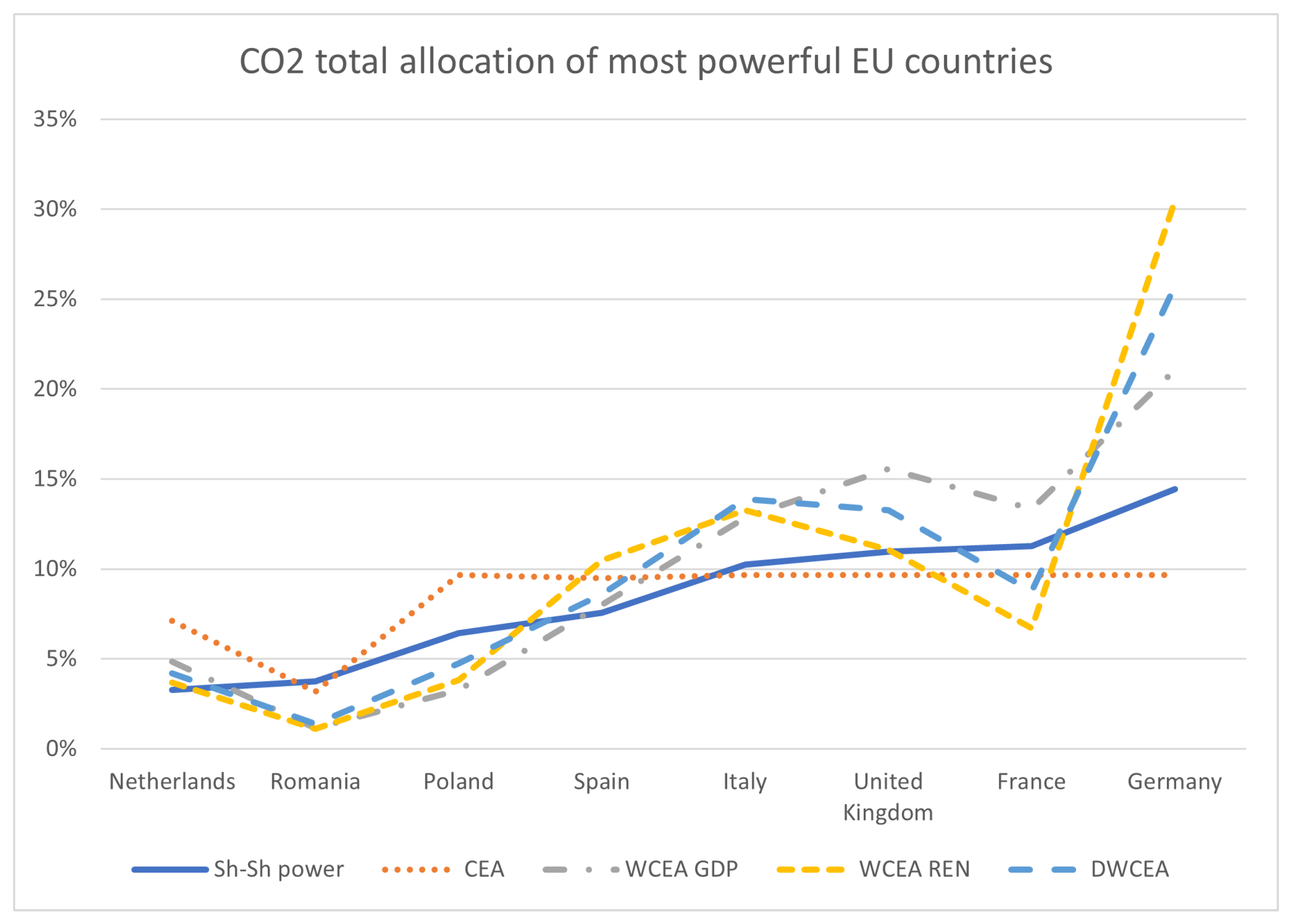
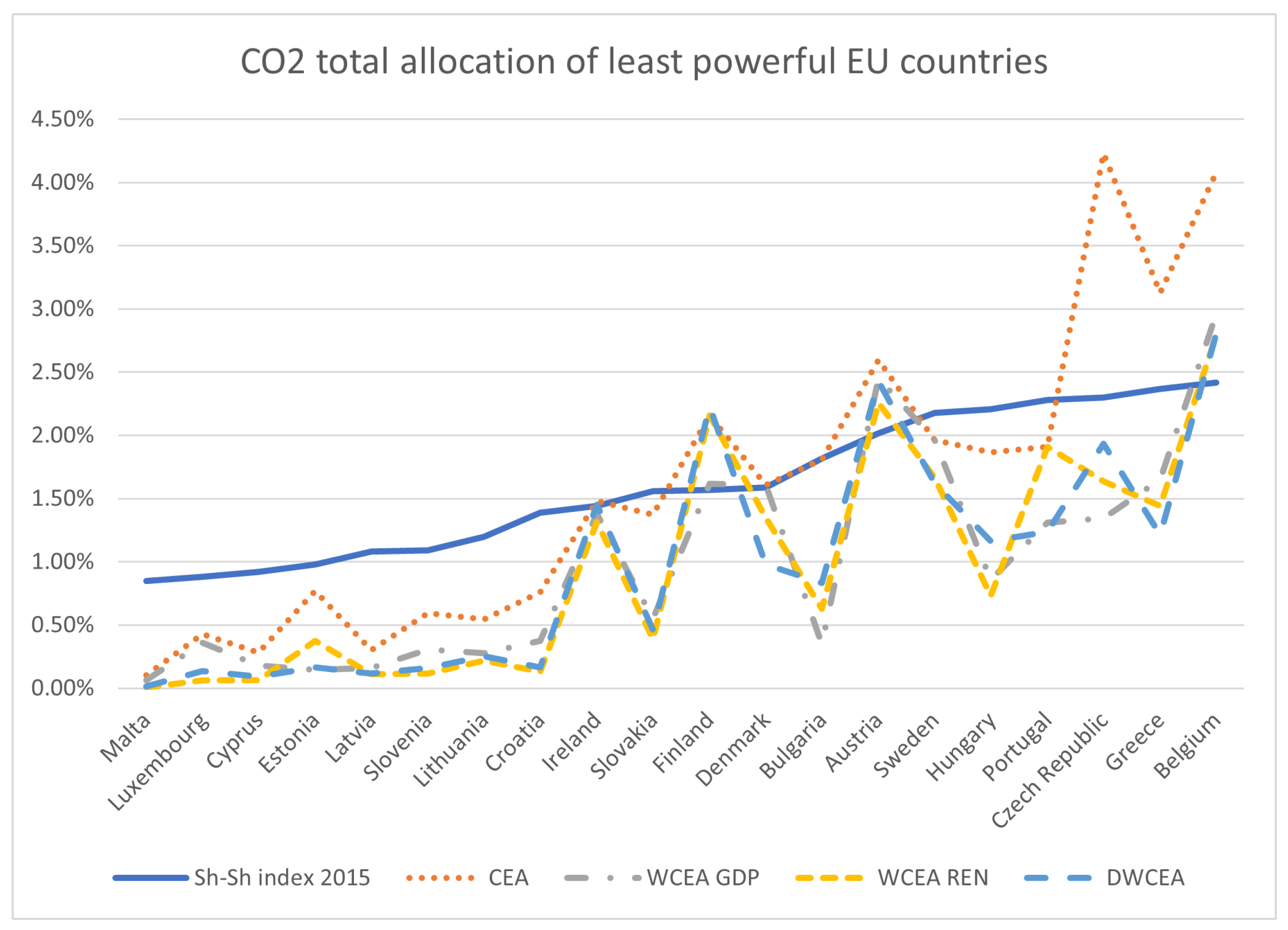
Figure 2 and Figure 3 show the distribution (in percentage) of total CO2 allocation vectors over the five years for the most powerful EU countries and the least powerful ones, respectively. In Figure 2, we observe the systematic cut operated by the CEA rule (dotted line) on the demand of CO2 permits for the six most powerful countries (precisely, for Poland, Spain, Italy, UK, France, and Germany), while the the adoption of the DWCEA rule shows an increase of the association between the allocation of CO2 and the Sh–Sh power index of more than in terms of the Pearson correlation (see Table 5 for the correlation coefficients of the different CO2 allocation vectors versus the Sh–Sh index vector). On the other hand, for the group of countries with Sh–Sh index smaller than , the loss of correlation with the Sh–Sh power index faced by the DWCEA allocation with respect to the CEA allocation is much less important, and is in the order of (see Table 5). So, we argue that the loss of acceptability of the DWCEA versus the CEA for the groups of less powerful countries, is largely compensated by the double gain of acceptability for the most powerful ones, and further justified by the use of criteria based on production efficiency and environmental preservation, which may further encourage small countries to adopt better technologies to improve their energetic policies.
5. Conclusions
The most critical objective in climate change study is to encourage countries worldwide to limit their emissions by finding a common strategy. In our work, we propose a new bi-criteria method in order to allocate CO2 emissions permits in EU countries. The DWCEA method, by giving the same importance to two parameters (GDP and production of renewable energy), ensures a balance between efficiency and green policies. Using basic clustering techniques on allocation records over the years 2010–2014, we showed that the DWCEA allocation method generates allocation distributions over time, having similar behaviours within clusters of countries characterized by specific levels of decision influence within the EU Council voting system, and prevent the cluster of larger countries from claiming extra shares of emissions permits.
We also showed that the allocation suggested by the DWCEA solution could encounter a larger level of acceptability, with respect to another solution, by the most influential or powerful EU countries (according to the well established Shapley and Shubik measure of power [16]), and without drastically affecting the acceptability by less influential countries. The justification of the trade-off in favour of the larger and most powerful countries is based on the use of criteria aimed at taking into account both production efficiency and environmental preservation.
We want to stress the fact that the GDP parameter, which we use extensively in this preliminary application to estimate the production of a country, is not necessarily the most appropriate attribute to represent the sustainable growth of a country. We leave for future research the use of alternative criteria, more oriented to reward an eco-friendly production.
Finally, future research devoted to a more detailed analysis of the axiomatic foundation of the allocation rule defined according to Algorithm 1 would be relevant. In particular, considering the variability of the parameters involved in each production process, it would be interesting to study the monotonicity property of the solution with respect to changes in countries’ claims, populations, and in the two weights describing the evolving environmental policies of countries.
Author Contributions
R.T. carried out algorithm conception and implementation, data acquisition, and data analysis. S.M. drafted a first version of the article. All authors contributed to the interpretation of the results. All authors have read and agreed to the published version of the manuscript.
Funding
This research received no external funding.
Institutional Review Board Statement
Not applicable.
Informed Consent Statement
Not applicable.
Data Availability Statement
Data supporting reported results were essentially collected from the World Bank Open Data project: https://data.worldbank.org/indicator/ (accessed on 6 September 2021).
Conflicts of Interest
The authors declare no conflict of interest.
Appendix A
In this Appendix section, we provide the pseudo-code of all relevant routines and functions that are used by Algorithm 1 to compute an allocation according to the DWCEA solution introduced in Section 3.
| Algorithm A1. Allocations’ sum is higher than Estate |
Input: Estate E, Set of players N, Claims vector c, weight vectors , Output: an allocation vector while and do It ++; Bloc 2: if then else end if End Bloc 2 ForEach : if then ForEach : end if if then LastComputing end if end while return x |
| Algorithm A2. Estate is higher than allocations’ sum |
Input: Estate E, Set of players N, Claims vector c, weight vectors , Output: an allocation vector while and do It ++; Bloc 3: if then else end if End Bloc 3 ForEach : if then ForEach :
end if
if then LastComputing end if end while return x |
| Algorithm A3. LastComputing Algorithm DWCEA |
Input: Estate E, Set of players N, Claims vector c, weight vectors , Output: an allocation vector if OR then else end if return x |
| Algorithm A4. Function First for or |
Input: , : a vector of sorted for or Output: X if then %We are looking for the first while do end while else %We are looking for the first while do end while end if return X |
Appendix B

Table A1.
Parameters computed at each the iteration of Algorithm 1 on the double-weighted bankruptcy situation of Example 2, with and .
Table A1.
Parameters computed at each the iteration of Algorithm 1 on the double-weighted bankruptcy situation of Example 2, with and .
| : | ||||
| Agent | ||||
| 1 | 6 | 6 | ||
| 2 | 10 | 6.5 | ||
| 3 | 20 | 16.25 | ||
| : , , | ||||
| Agent | ||||
| 1 | 6 | 6 | ||
| 2 | 10 | 6.5 | ||
| 3 | 20 | 20 | ||
| LastComputing Process: , | ||||
| Agent | ||||
| 1 | 6 | 6 | ||
| 2 | 10 | 6.5 | ||
| 3 | 20 | 17.5 | ||
Table A2.
Allocation vectors provided by CEA solution for each year in the interval 2010–2014 (values are in millions of tons of CO2).
Table A2.
Allocation vectors provided by CEA solution for each year in the interval 2010–2014 (values are in millions of tons of CO2).
| Country | CEA2010 | CEA2011 | CEA2012 | CEA2013 | CEA2014 |
|---|---|---|---|---|---|
| Austria | 67.502 | 65.02 | 62.273 | 62.486 | 58.712 |
| Belgium | 110.824 | 99.944 | 95.107 | 96.97 | 93.351 |
| Bulgaria | 44.114 | 49.347 | 44.708 | 39.6 | 42.416 |
| Croatia | 20.172 | 19.809 | 17.994 | 17.55 | 16.843 |
| Cyprus | 7.708 | 7.426 | 6.92 | 5.948 | 6.062 |
| Czech republic | 111.579 | 106.908 | 101.03 | 98.675 | 96.475 |
| Denmark | 46.641 | 40.645 | 36.428 | 38.533 | 33.498 |
| Estonia | 18.108 | 18.606 | 17.624 | 19.893 | 19.519 |
| Finland | 62.082 | 56.816 | 49.134 | 47.22 | 47.301 |
| France | 220.42 | 227.373 | 236.057 | 242.088 | 248.389 |
| Germany | 220.42 | 227.373 | 236.057 | 242.088 | 248.389 |
| Greece | 83.857 | 79.842 | 80.043 | 69.482 | 67.319 |
| Hungary | 50.233 | 47.843 | 44.583 | 42.141 | 42.086 |
| Ireland | 40.055 | 35.632 | 35.592 | 34.855 | 34.066 |
| Italy | 220.42 | 227.373 | 236.057 | 242.088 | 248.389 |
| Lativia | 8.075 | 7.294 | 7.063 | 7.081 | 6.975 |
| Lithuania | 13.469 | 13.788 | 13.832 | 12.64 | 12.838 |
| luxembourg | 10.968 | 10.939 | 10.664 | 10.051 | 9.659 |
| Malta | 2.56 | 2.541 | 2.681 | 2.34 | 2.347 |
| Netherlands | 183.053 | 174.168 | 170.31 | 173.255 | 167.303 |
| Poland | 220.42 | 227.373 | 236.057 | 242.088 | 248.389 |
| Portugal | 48.137 | 47.623 | 46.014 | 45.427 | 45.053 |
| Romania | 79.413 | 84.88 | 81.723 | 70.945 | 70.003 |
| Slovakia | 36.241 | 34.525 | 32.765 | 33.091 | 30.678 |
| Slovenia | 15.335 | 15.09 | 14.782 | 14.151 | 12.812 |
| Spain | 220.42 | 227.373 | 236.057 | 237.035 | 233.977 |
| Sweden | 52.024 | 51.734 | 47.048 | 44.847 | 43.421 |
| UK | 220.42 | 227.373 | 236.057 | 242.088 | 248.389 |
Table A3.
Allocation vectors provided by the WCEA solution with GDP as a unique weight (denoted by WCEA1) for each year in the interval 2010–2014 (values are in millions of tons of CO2).
Table A3.
Allocation vectors provided by the WCEA solution with GDP as a unique weight (denoted by WCEA1) for each year in the interval 2010–2014 (values are in millions of tons of CO2).
| Country | WCEA2010 | WCEA2011 | WCEA2012 | WCEA2013 | WCEA2014 |
|---|---|---|---|---|---|
| Austria | 57.417 | 59.44 | 60.14 | 62.486 | 58.712 |
| Belgium | 70.846 | 72.66 | 73.134 | 69.482 | 73.843 |
| Bulgaria | 7.415 | 7.916 | 7.918 | 11.258 | 7.893 |
| Croatia | 8.766 | 8.6 | 8.325 | 11.728 | 8.018 |
| Cyprus | 3.745 | 3.781 | 4.131 | 5.948 | 4.359 |
| Czech republic | 30.398 | 31.428 | 30.461 | 42.28 | 28.912 |
| Denmark | 46.641 | 40.645 | 36.428 | 38.533 | 33.498 |
| Estonia | 2.856 | 3.195 | 3.385 | 5.075 | 3.25 |
| Finland | 36.306 | 37.732 | 37.707 | 47.22 | 37.926 |
| France | 353.033 | 331.805 | 333.228 | 302.278 | 303.276 |
| Germany | 500.647 | 518.086 | 520.573 | 485.25 | 541.275 |
| Greece | 43.86 | 39.68 | 36.086 | 48.43 | 32.976 |
| Hungary | 19.182 | 19.41 | 18.781 | 27.301 | 19.494 |
| Ireland | 32.519 | 32.954 | 33.134 | 34.855 | 34.066 |
| Italy | 311.348 | 313.84 | 304.476 | 334.097 | 299.357 |
| Lativia | 3.481 | 3.891 | 3.678 | 4.863 | 3.648 |
| Lithuania | 5.439 | 5.994 | 6.294 | 9.372 | 6.75 |
| luxembourg | 7.796 | 8.273 | 8.309 | 10.51 | 9.228 |
| Malta | 1.281 | 1.311 | 1.353 | 2.048 | 1.563 |
| Netherlands | 122.542 | 123.225 | 121.763 | 98.675 | 122.378 |
| Poland | 70.227 | 72.912 | 73.498 | 105.847 | 75.847 |
| Portugal | 34.914 | 33.764 | 31.782 | 27.302 | 31.947 |
| Romania | 24.418 | 25.419 | 25.216 | 38.675 | 27.754 |
| Slovakia | 13.113 | 13.537 | 13.722 | 19.883 | 6.943 |
| Slovenia | 7.035 | 7.072 | 6.809 | 9.715 | 6.943 |
| Spain | 209.75 | 205.165 | 196.247 | 173.255 | 191.561 |
| Sweden | 52.024 | 51.734 | 47.048 | 44.847 | 43.421 |
| UK | 357.657 | 361.187 | 391.03 | 363.443 | 419.818 |
Table A4.
Allocation vectors provided by the WCEA solution with renewable energy production as a unique weight (denoted by WCEA2) for each year in the interval 2010–2014 (values are in millions of tons of CO2).
Table A4.
Allocation vectors provided by the WCEA solution with renewable energy production as a unique weight (denoted by WCEA2) for each year in the interval 2010–2014 (values are in millions of tons of CO2).
| Country Name | WCEA2010 | WCEA2011 | WCEA2012 | WCEA2013 | WCEA2014 |
|---|---|---|---|---|---|
| Austria | 67.502 | 58.9690341 | 50.3242476 | 48.6899831 | 49.2450121 |
| Belgium | 66.5044105 | 72.7969923 | 68.6554869 | 66.0842777 | 65.7096249 |
| Bulgaria | 7.86391525 | 22.1211738 | 14.2802869 | 16.645398 | 15.3401465 |
| Croatia | 1.850333 | 2.2779648 | 2.8886825 | 3.82054302 | 5.1262437 |
| Cyprus | 0.78531575 | 1.5838974 | 1.7468033 | 1.91319689 | 1.74733253 |
| Czech republic | 33.4888758 | 47.0275155 | 40.3463984 | 38.4687141 | 40.0343097 |
| Denmark | 46.641 | 9.0584694 | 36.428 | 38.533 | 33.498 |
| Estonia | 10.9406318 | 10.2241467 | 9.7535515 | 6.98580147 | 7.50746658 |
| Finland | 62.082 | 56.816 | 49.134 | 47.22 | 47.301 |
| France | 166.551486 | 174.477866 | 165.300608 | 151.862197 | 159.723832 |
| Germany | 758.86 | 732.498 | 739.861 | 756.900473 | 719.883 |
| Greece | 32.9402305 | 14.1216021 | 39.0685812 | 46.8235923 | 42.4486051 |
| Hungary | 30.465948 | 11.1896123 | 16.5368577 | 15.0656941 | 15.6488235 |
| Ireland | 33.6609998 | 35.632 | 30.2733926 | 29.4234469 | 31.3141833 |
| Italy | 278.07708 | 330.482862 | 342.210321 | 345.318 | 320.411 |
| Latvia | 1.23714125 | 1.690677 | 2.7323538 | 3.63916961 | 4.4647929 |
| Lithuania | 3.99112525 | 5.6237256 | 5.165644 | 5.88000878 | 6.12944408 |
| Luxembourg | 1.71048225 | 1.6372872 | 1.4205521 | 1.46853951 | 1.60401819 |
| Malta | 0.01075775 | 0.088983 | 0.1767194 | 0.20477643 | 0.41340675 |
| Netherlands | 119.324963 | 109.13765 | 84.349529 | 70.6127621 | 63.9181956 |
| Poland | 85.717752 | 96.1550298 | 100.87959 | 85.5848441 | 97.3435094 |
| Portugal | 48.137 | 47.623 | 46.014 | 45.427 | 45.053 |
| Romania | 4.48598175 | 36.7677756 | 19.439134 | 30.37712 | 45.871613 |
| Slovakia | 7.36905875 | 10.8648243 | 9.3185499 | 8.80538628 | 11.1344218 |
| Slovenia | 2.48504025 | 2.8296594 | 2.922667 | 2.81421316 | 2.86077471 |
| Spain | 270.911 | 270.548 | 264.779 | 237.035 | 233.977 |
| Sweden | 52.024 | 15.6832538 | 47.048 | 44.847 | 43.421 |
| UK | 239.037472 | 256.728998 | 243.602043 | 284.205863 | 323.526244 |
Table A5.
Allocation vectors provided by the DWCEA solution for each year in the interval 2010–2014 (values are in millions of tons of CO2).
Table A5.
Allocation vectors provided by the DWCEA solution for each year in the interval 2010–2014 (values are in millions of tons of CO2).
| Country | DWCEA2010 | DWCEA2011 | DWCEA2012 | DWCEA2013 | DWCEA2014 |
|---|---|---|---|---|---|
| Austria | 67.5 | 65.02 | 59.2867896 | 44.8095231 | 58.712 |
| Belgium | 72.61 | 82.104421 | 80.8827474 | 31.7920563 | 73.5489375 |
| Bulgaria | 8.59 | 10.0119837 | 36.428 | 38.533 | 7.86135324 |
| Croatia | 2.02 | 2.56921303 | 3.403145 | 4.17207565 | 7.9857891 |
| Cyprus | 0.86 | 1.78640593 | 2.0579018 | 2.39828374 | 4.34209095 |
| Czech republic | 36.56 | 39.7473206 | 47.5319264 | 82.8398009 | 28.7973403 |
| Denmark | 46.64 | 10.2166362 | 19.4820042 | 9.25451589 | 33.498 |
| Estonia | 3.9 | 4.04015573 | 4.10746293 | 4.78923329 | 3.23685663 |
| Finland | 49.56 | 47.7205688 | 48.7808458 | 87.0089472 | 37.7754291 |
| France | 181.84 | 196.78566 | 194.739968 | 190.366523 | 303.276 |
| Germany | 683.42 | 655.230259 | 631.695144 | 622.817849 | 539.121412 |
| Greece | 35.96 | 15.9271136 | 22.901164 | 39.8107335 | 32.8452471 |
| Hungary | 26.18 | 12.6202554 | 38.5663747 | 44.847 | 19.4161707 |
| Ireland | 36.75 | 35.632 | 35.592 | 34.855 | 34.066 |
| Italy | 303.6 | 372.736609 | 369.469 | 345.318 | 298.165642 |
| Latvia | 1.35 | 1.90683779 | 3.2189748 | 3.99747153 | 3.63399825 |
| Lithuania | 4.36 | 6.34274466 | 6.085624 | 7.37087206 | 6.72286212 |
| luxembourg | 1.87 | 1.84662186 | 1.6735466 | 1.84088446 | 9.19093239 |
| Malta | 0.01 | 0.1 | 0.2081924 | 0.25669704 | 1.55669538 |
| Netherlands | 130.28 | 123.091398 | 99.371834 | 34.755181 | 121.891022 |
| Poland | 93.58 | 92.2125004 | 89.186524 | 226.031663 | 75.5455926 |
| Portugal | 47.66 | 42.702371 | 9.6079055 | 18.8855677 | 31.8198291 |
| Romania | 4.9 | 32.1480963 | 43.7894691 | 61.0352212 | 27.643745 |
| Slovakia | 8.05 | 12.2539418 | 10.9781454 | 11.0379726 | 13.9883644 |
| Slovenia | 2.71 | 3.19144431 | 3.443182 | 3.52775071 | 6.91533585 |
| Spain | 270.91 | 259.474424 | 238.137846 | 88.5164725 | 190.798557 |
| Sweden | 52.02 | 17.6884295 | 47.048 | 37.5221251 | 43.421 |
| UK | 260.966 | 289.548588 | 286.982282 | 356.26558 | 418.879797 |
| 1 | https://www.unep.org/interactive/emissions-gap-report/2020/ (accessed on 6 September 2021). |
| 2 | https://www.nytimes.com/2020/08/19/climate/earth-overshoot-day.html (accessed on 6 September 2021). |
| 3 | https://data.worldbank.org/indicator/ (accessed on 6 September 2021). |
| 4 | https://www.consilium.europa.eu/fr/council-eu/voting-system/voting-calculator/ (accessed on 6 September 2021). |
References
- Jin, Z.-G.; Cai, W.-J.; Wang, C. Simulation of climate negotiation strategies between China and the US based on game theory. Adv. Clim. Chang. Res. 2014, 5, 34–40. [Google Scholar] [CrossRef]
- Zhou, P.; Wang, M. Carbon dioxide emissions allocation: A review. Ecol. Econ. 2016, 125, 47–59. [Google Scholar] [CrossRef]
- Rose, A.; Zhang, Z.X. Interregional burden-sharing of greenhouse gas mitigation in the United States. Mitig. Adapt. Strateg. Glob. Chang. 2004, 9, 477–500. [Google Scholar] [CrossRef] [Green Version]
- Zhou, P.; Sun, Z.R.; Zhou, D.Q. Optimal path for controlling CO2 emissions in China: A perspective of efficiency analysis. Energy Econ. 2014, 45, 99–110. [Google Scholar] [CrossRef]
- Duro, J.A.; Giménez-Gómez, J.M.; Vilella, C. The allocation of CO2 emissions as a claims problem. Energy Econ. 2020, 86, 104652. [Google Scholar] [CrossRef] [Green Version]
- Giménez-Gómez, J.M.; Teixidó-Figueras, J.; Vilella, C. The global carbon budget: A conflicting claims problem. Clim. Chang. 2016, 136, 693–703. [Google Scholar] [CrossRef] [Green Version]
- O’Neill, B. A problem of rights arbitration from the Talmud. Math. Soc. Sci. 1982, 2, 345–371. [Google Scholar] [CrossRef] [Green Version]
- Thomson, W. Axiomatic and game-theoretic analysis of bankruptcy and taxation problems: A survey. Math. Soc. Sci. 2003, 45, 249–297. [Google Scholar] [CrossRef]
- Thomson, W. Axiomatic and game-theoretic analysis of bankruptcy and taxation problems: An update. Math. Soc. Sci. 2015, 74, 41–59. [Google Scholar] [CrossRef] [Green Version]
- Madani, K.; Zarezadeh, M. Bankruptcy methods for resolving water resources conflicts. In Proceedings of the World Environmental and Water Resources Congress: Crossing Boundaries, Albuquerque, Mexico, 20–24 May 2012. [Google Scholar]
- Aumann, R.J.; Maschler, M. Game theoretic analysis of a bankruptcy problem from the Talmud. J. Econ. Theory 1985, 36, 195–213. [Google Scholar] [CrossRef]
- Casas-Méndez, B.; Fragnelli, V.; García-Jurado, I. Weighted bankruptcy rules and the museum pass problem. Eur. J. Oper. Res. 2011, 215, 161–168. [Google Scholar] [CrossRef]
- Moulin, H. Priority rules and other asymmetric rationing methods. Econometrica 2000, 68, 643–684. [Google Scholar] [CrossRef]
- Trabelsi, R.; Moretti, S.; Krichen, S. Using Bankruptcy Rules to Allocate CO2 Emission Permits. In International Conference on Game Theory for Networks; Springer: Cham, Switzerland, 2019. [Google Scholar]
- Thomson, W. How to Divide When There Isn’t Enough. No. 62; Cambridge University Press: Cambridge, UK, 2019. [Google Scholar]
- Shapley, L.S.; Shubik, M. A method for evaluating the distribution of power in a committee system. Am. Political Sci. Rev. 1954, 48, 787–792. [Google Scholar] [CrossRef]
- Kóczy, L.Á. Brexit and Power in the Council of the European Union. Games 2021, 12, 51. [Google Scholar] [CrossRef]
- Felsenthal, D.S. A well-behaved index of a priori p-power for simple n-person games. Homo Oeconomicus 2016, 33, 367–381. [Google Scholar] [CrossRef]
- Vesterdal, M.; Svendsen, G.T. How should greenhouse gas permits be allocated in the EU? Energy Policy 2004, 32, 961–968. [Google Scholar] [CrossRef]
- Sinwar, D.; Kaushik, R. Study of Euclidean and Manhattan distance metrics using simple k-means clustering. Int. J. Res. Appl. Sci. Eng. Technol. 2014, 2, 270–274. [Google Scholar]
Figure 1.
Percentage distribution of total EU CO2 emissions, GPD and renewable energy production of each EU country over the interval time of five years from 2010 to 2014 (all data were collected from the World Bank Open Data project in 2020, see https://data.worldbank.org/indicator/EN.ATM.CO2E.KT?view=chart (accessed on 6 September 2021)).

Figure 2.
Percentages of total CO2 emissions permits for the eight most powerful countries (Sh–Sh power index ) for the four allocation rules considered in this paper. Countries are ordered according to the Sh–Sh power index (solid line).
Figure 2.
Percentages of total CO2 emissions permits for the eight most powerful countries (Sh–Sh power index ) for the four allocation rules considered in this paper. Countries are ordered according to the Sh–Sh power index (solid line).

Figure 3.
Percentages of total CO2 emission permits for EU countries with Sh–Sh power index strictly smaller than for the four allocation rules considered in this paper. Countries are ordered according to the Sh–Sh power index (solid line).
Figure 3.
Percentages of total CO2 emission permits for EU countries with Sh–Sh power index strictly smaller than for the four allocation rules considered in this paper. Countries are ordered according to the Sh–Sh power index (solid line).

Table 1.
A double-weighted bankruptcy situation with as set of agents and estate .
| Agent i | |||||
|---|---|---|---|---|---|
| 1 | 6 | 3 | 2 | 12 | |
| 2 | 10 | 2 | 5 | 2 | 5 |
| 3 | 20 | 8 | 5 | 4 |
Table 2.
Parameters computed at each the iteration of Algorithm 1 on the double-weighted bankruptcy situation of Example 1, with and .
Table 2.
Parameters computed at each the iteration of Algorithm 1 on the double-weighted bankruptcy situation of Example 1, with and .
| : | ||||
| Agent | ||||
| 1 | 6 | 6 | ||
| 2 | 10 | |||
| 3 | 20 | |||
| : , , | ||||
| Agent | ||||
| 1 | 6 | 6 | ||
| 2 | 10 | 5 | ||
| 3 | 20 | |||
| : , , | ||||
| Agent | ||||
| 1 | 6 | 6 | ||
| 2 | 10 | 4 | ||
| 3 | 20 | 16 | ||
| : , , | ||||
| Agent | ||||
| 1 | 6 | 6 | ||
| 2 | 10 | 1 | ||
| 3 | 20 | |||
| LastComputing Process: , | ||||
| Agent | ||||
| 1 | 6 | 6 | ||
| 2 | 10 | 4 | ||
| 3 | 20 | 10 | ||
Table 3.
Outcomes of the K-means clustering application over allocation records provided by alternative allocation methods. Names in bold indicate countries that are totally satisfied at least for 3 years.
Table 3.
Outcomes of the K-means clustering application over allocation records provided by alternative allocation methods. Names in bold indicate countries that are totally satisfied at least for 3 years.
| Table 3(1): Clustering EU country emissions | Maps: EU country emissions | ||
| Group 1 | Group 2 | Group 3 |  |
| Malta | Romania | Spain | |
| Cyprus | Greece | Poland | |
| Latvia | Belgium | France | |
| Luxembourg | Czech republic | Italy | |
| Lithuania | Netherlands | Germany | |
| Slovenia | |||
| Estonia | |||
| Croatia | |||
| Slovakia | |||
| Ireland | |||
| Bulgaria | |||
| Denmark | |||
| Portugal | |||
| Hungary | |||
| Sweden | |||
| Finland | |||
| Austria | |||
| Table 3(2): Clustering CEA allocations | Maps: CEA allocations | ||
| Group 1 | Group 2 | Group 3 |  |
| Malta | Romania | Netherlands | |
| Cyprus | Greece | Poland | |
| Latvia | Belgium | France | |
| Luxembourg | Czech republic | Italy | |
| Lithuania | Denmark | Germany | |
| Slovenia | Bulgaria | Spain | |
| Estonia | Portugal | ||
| Croatia | Hungary | ||
| Slovakia | Sweden | ||
| Ireland | Finland | ||
| Austria | |||
| Table 3(3): Clustering WCEA GDP allocations | Maps: WCEA GDP allocations | ||
| Group 1 | Group 2 | Group 3 |  |
| Malta | Austria | Spain | |
| Cyprus | Greece | France | |
| Latvia | Belgium | Italy | |
| Luxembourg | Czech republic | Germany | |
| Lithuania | Netherlands | ||
| Slovenia | Poland | ||
| Estonia | Ireland | ||
| Croatia | Denmark | ||
| Slovakia | Portugal | ||
| Bulgaria | Sweden | ||
| Romania | Finland | ||
| Hungary | |||
| Table 3(4): Clustering WCEA renewable energy | Maps: WCEA renewable energy | ||
| Group 1 | Group 2 | Group 3 |  |
| Malta | Austria | Italy | |
| Cyprus | Greece | Spain | |
| Latvia | Belgium | Germany | |
| Luxembourg | Czech republic | ||
| Lithuania | Netherlands | ||
| Slovenia | Poland | ||
| Estonia | Finland | ||
| Croatia | Denmark | ||
| Slovakia | Portugal | ||
| Bulgaria | Sweden | ||
| Hungary | France | ||
| Ireland | Romania | ||
| Table 3(5): Clustering DWCEA allocations | Maps: DWCEA allocations | ||
| Group 1 | Group 2 | Group 3 |  |
| Malta | Austria | Italy | |
| Cyprus | Greece | Spain | |
| Latvia | Belgium | Germany | |
| Luxembourg | Czech republic | France | |
| Lithuania | Netherlands | ||
| Slovenia | Poland | ||
| Estonia | Finland | ||
| Croatia | Denmark | ||
| Slovakia | Portugal | ||
| Bulgaria | Sweden | ||
| Hungary | |||
| Ireland | |||
| Romania | |||
Table 4.
Cluster combinations that are able to approve a decision according to the EU Council voting systems.
Table 4.
Cluster combinations that are able to approve a decision according to the EU Council voting systems.
| Emissions | CEA | WCEA | WCEA | DWCEA |
|---|---|---|---|---|
| G1 + G3 | G1 + G3 | G1 + G3 | G1 + G2 | G1 + G2 |
| G1 + G2 + G3 | G2 + G3 | G2 + G3 | G1 + G2 + G3 | G1 + G2 + G3 |
| G1 + G2 + G3 | G1 + G2 + G3 |
Table 5.
Pearson correlation coefficients for CO2 allocation vectors provided by the four allocation rules considered in this paper over the interval 2010–2014, and for two groups of countries (groups are based on the Sh–Sh power index, cut-off ).
Table 5.
Pearson correlation coefficients for CO2 allocation vectors provided by the four allocation rules considered in this paper over the interval 2010–2014, and for two groups of countries (groups are based on the Sh–Sh power index, cut-off ).
| CEA | WCEA | WCEA | DWCEA | |
|---|---|---|---|---|
| 8 EU countries (Sh–Sh ) | 0.69 | 0.95 | 0.82 | 0.90 |
| 17 EU countries (Sh–Sh ) | 0.89 | 0.77 | 0.79 | 0.78 |
Publisher’s Note: MDPI stays neutral with regard to jurisdictional claims in published maps and institutional affiliations. |
© 2021 by the authors. Licensee MDPI, Basel, Switzerland. This article is an open access article distributed under the terms and conditions of the Creative Commons Attribution (CC BY) license (https://creativecommons.org/licenses/by/4.0/).
Share and Cite
MDPI and ACS Style
Moretti, S.; Trabelsi, R. A Double-Weighted Bankruptcy Method to Allocate CO2 Emissions Permits. Games 2021, 12, 78. https://0-doi-org.brum.beds.ac.uk/10.3390/g12040078
AMA Style
Moretti S, Trabelsi R. A Double-Weighted Bankruptcy Method to Allocate CO2 Emissions Permits. Games. 2021; 12(4):78. https://0-doi-org.brum.beds.ac.uk/10.3390/g12040078
Chicago/Turabian StyleMoretti, Stefano, and Raja Trabelsi. 2021. "A Double-Weighted Bankruptcy Method to Allocate CO2 Emissions Permits" Games 12, no. 4: 78. https://0-doi-org.brum.beds.ac.uk/10.3390/g12040078
Note that from the first issue of 2016, this journal uses article numbers instead of page numbers. See further details here.