
Optimal Accuracy of Unbiased Tullock Contests with Two Heterogeneous Players


1
Department of Economics, Otto-Friedrich-Universität Bamberg, Feldkirchenstraße 21, 96052 Bamberg, Germany
2
CESifo, Poschingerstraße 5, 81679 Munich, Germany
Games 2022, 13(2), 24; https://0-doi-org.brum.beds.ac.uk/10.3390/g13020024
Submission received: 8 March 2022
/
Revised: 18 March 2022
/
Accepted: 24 March 2022
/
Published: 25 March 2022
(This article belongs to the Special Issue Advances in the Theory and Applications of Contests and Tournaments)
Abstract
:I characterize the optimal accuracy level r of an unbiased Tullock contest between two players with heterogeneous prize valuations. The designer maximizes the winning probability of the strong player or the winner’s expected valuation by choosing a contest with an all-pay auction equilibrium (). By contrast, if she aims at maximizing the expected aggregate effort or the winner’s expected effort, she will choose a contest with a pure-strategy equilibrium, and the optimal accuracy level decreases in the players’ heterogeneity. Finally, a contest designer who faces a tradeoff between selection quality and minimum (maximum) effort will never choose a contest with a semi-mixed equilibrium.
Keywords:
Tullock contest; heterogeneous valuations; accuracy; discrimination; optimal design; all-pay auctionJEL Classification:
C72; D721. Introduction
I characterize the optimal accuracy level, sometimes also referred to as decisiveness parameter or discriminatory power, of an unbiased Tullock contest between two players with heterogeneous prize valuations under different objectives. As the accuracy level affects efforts, winning probabilities, and payoffs, it is an important tool for designing a contest, particularly when an explicit bias or affirmative action is not feasible. Real world examples are countless and range from defining the type and size of the jury in litigation (number of jurors/judges)1 to specifying the rules in sports like car racing (technical limitations)2, table tennis (size of the ball)3, or soccer (tie breaking regulations)4.
The analysis thus contributes to the large literature on (optimal) contest design. More specifically, it complements the articles that emphasize the role of the accuracy of the contest success function, e.g., Nti [5], Alcalde and Dahm [6], Wang [7], and, particularly, Ewerhart [8] and Chowdhury et al. [9]. Ewerhart [8] proves the uniqueness of the Nash equilibrium in two-player Tullock contests and applies this finding to provide the following ranking result: a designer who maximizes aggregate effort (i.e., revenue) and can optimally bias the contest always prefers the highest possible accuracy level. By contrast, I consider unbiased contests and use his uniqueness result to determine the optimal accuracy level with regard to different design objectives. For example, a designer who maximizes aggregate effort and cannot bias the contest always prefers to limit the level of accuracy (Proposition 2). In their comprehensive survey on heterogeneity and affirmative action in contests, Chowdhury et al. [9] make an analogous observation (see Observation 1.2.1 in [9]). I add to their contribution by providing an exact specification of the optimal accuracy level (Corollary 1) and considering alternative objectives (Propositions 1 and 3).
The paper is organized as follows. Section 2 introduces the formal set-up. In Section 3 and Section 4, I examine the optimal accuracy level under the assumptions that the designer maximizes the winning probability of the strong player, the winner’s expected valuation, the expected aggregate effort, and the winner’s expected effort, respectively. Section 5 discusses the optimal solution to different tradeoffs between selection quality and effort. Section 6 concludes.
2. Set-Up and Notation
I consider the standard model of a Tullock contest [10] between two players with linear effort costs and use the same notation as Ewerhart [8]. Player i’s probability of winning is
where denotes the effort of player and describes the accuracy level of the contest.5 Player chooses to maximize the payoff , where the players’ valuations for the prize are normalized to and . I thus refer to player 1 (2) as the strong (weak) player.
Propositions 1–4 in Ewerhart [8] show that, for any given ,
- there is a unique Nash equilibrium, which is in pure strategies, if ,
- there is a unique Nash equilibrium, which is in semi-mixed strategies, if ,
- any Nash equilibrium is an all-pay auction equilibrium (i.e., it yields the same expected efforts, winning probabilities and expected payoffs as well as the same expected revenue for the contest designer as the unique equilibrium of the corresponding all-pay auction) in mixed strategies if ,
where is an implicit function of defined by
Below, I mark equilibrium values with an asterisk where appropriate.
3. Maximization of Selection Quality
I first consider different objectives associated with the selection quality of the contest. Table 1 in Ewerhart [8] shows that for all we have if and if . Thus, for any , the designer maximizes the strong player’s winning probability by choosing any contest with an all-pay auction equilibrium (). Moreover, since the winner’s expected equilibrium valuation equals
and for all , a contest that maximizes the strong player’s winning probability also maximizes the winner’s expected valuation.
Proposition 1.
For any , the designer maximizes the the strong player’s winning probability (winner’s expected valuation) by choosing any contest with an all-pay auction equilibrium ().
4. Effort Maximization
I now consider different objectives associated with effort maximization.
4.1. Maximization of Aggregate Effort
For any , Nti [5] determines the accuracy level r that maximizes aggregate effort in the range of pure strategy equilibria, i.e., under the constraint . Alcalde and Dahm [6] show that for any , there exists an all-pay auction equilibrium, and for any , any equilibrium is an all-pay auction equilibrium. Epstein et al. [12] show that, for any , the accuracy level r that maximizes aggregate effort in the range of pure strategy equilibria also leads to a higher aggregate effort than an all-pay auction (). Wang [7] determines a semi-mixed equilibrium for all and shows that, within this class of equilibria, the aggregate equilibrium effort decreases in the accuracy level r for any , i.e., if . Finally, Ewerhart [8] shows that for any the equilibrium is unique.
Together, these results allow for a unique identification of the optimal accuracy level. More explicitly, Table 1 in Ewerhart [8] shows that for any , aggregate equilibrium effort is a continuous function of r. This implies that, for any , the optimal accuracy level must satisfy . It thus coincides with the optimal accuracy level within the region of pure-strategy equilibria as characterized by Nti [5]. I briefly summarize his analysis and add an exact equation for the threshold he approximates (cf. Table 1 and Proposition 3 in [5]).
For any , the optimal accuracy level r maximizes aggregate equilibrium effort subject to the constraint that . The first order condition for an unconstrained maximizer implies
Straightforward calculations show that , , and for all . As and F have the same sign, is inverted U-shaped and single-peaked. Moreover, for all . Thus, Equation (2) defines an implicit function satisfying for all . Notice from Equation (1) that is also an increasing function of .
Proposition 2.
For any , aggregate effort is an inverted U-shaped function of the accuracy level. The designer maximizes aggregate effort by choosing a contest with a pure-strategy equilibrium. The optimal accuracy level equals and decreases as the players’ heterogeneity increases: .6
Inserting into Equation (2) implies
It is straightforward to show that f is strictly increasing for all and has a unique root which I denote by . Therefore, if and only if or, equivalently, , where
Corollary 1.
The designer maximizes aggregate effort by choosing
- (a)
- if ,
- (b)
- if .
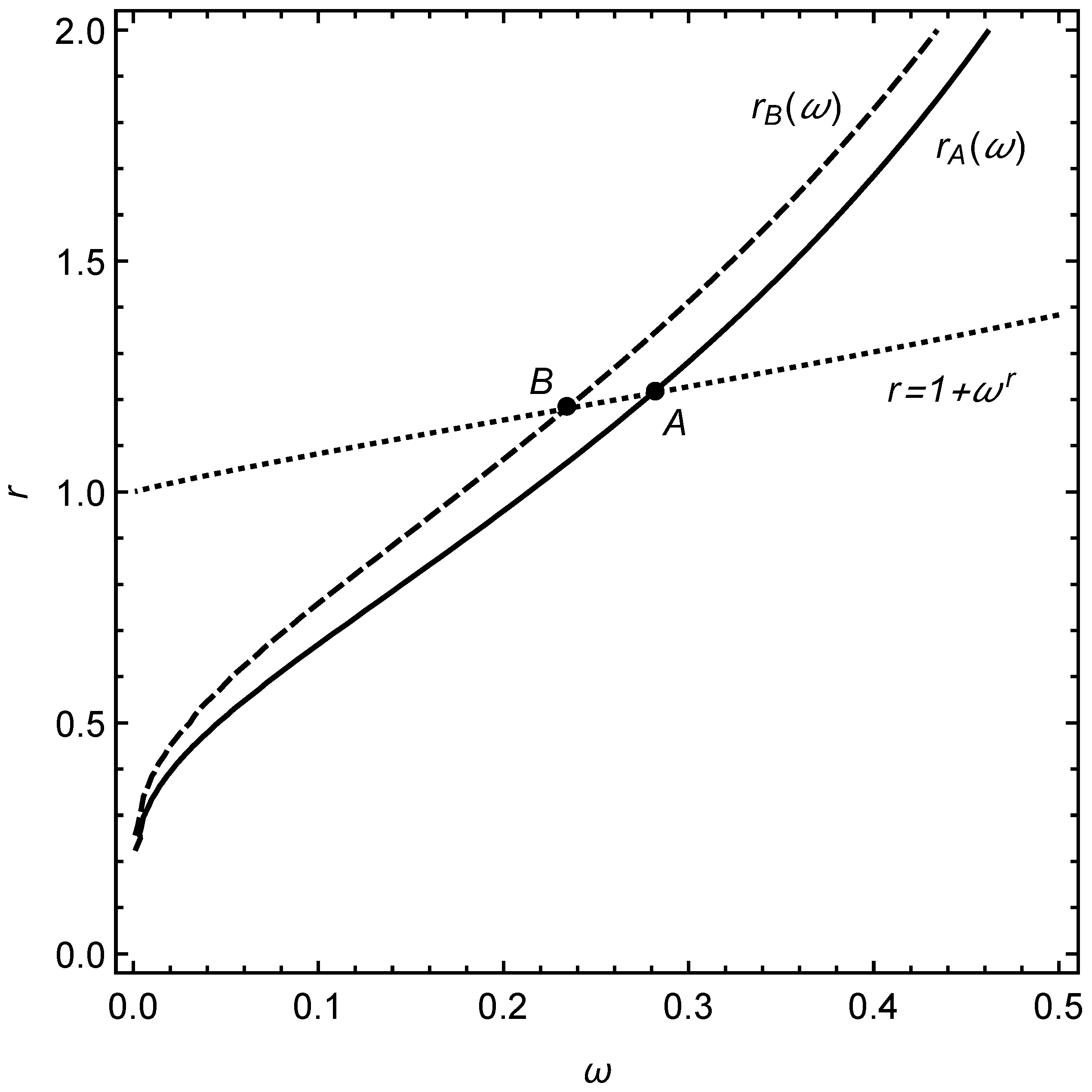
Figure 1 illustrates Proposition 2 and Corollary 1. The solid (dotted) curve depicts () as a function of . The curves intersect at some point to the left (right) of which the optimal accuracy level is unconstrained (constrained).
4.2. Maximization of the Winner’s Expected Effort
Straightforward calculations show that, for all , the winner’s expected equilibrium effort is also a continuous function of r with for . Again, these observations imply that, for any , the optimal accuracy level must satisfy and thus coincides with the optimal accuracy level within the region of pure-strategy equilibria.
For any , the optimal accuracy level r maximizes the winner’s expected equilibrium effort subject to the constraint that . The first order condition for an unconstrained maximizer implies
Straightforward calculations show that , , and for all . As and G have the same sign, is inverted U-shaped and single-peaked.
Proposition 3.
For any , the winner’s expected effort is an inverted U-shaped function of the accuracy level. The designer maximizes the winner’s expected effort by choosing a contest with a pure-strategy equilibrium. The optimal accuracy level equals .
Moreover, numerical approximations suggest for all , i.e., the optimal accuracy level decreases as the players’ heterogeneity increases.
Inserting into Equation (2) implies
One can show that g is strictly increasing7 and has a unique root which I denote by . Therefore, if and only if or, equivalently, , where
Corollary 2.
The designer maximizes the winner’s expected effort by choosing
- (a)
- if ,
- (b)
- if .
Figure 1 illustrates Proposition 3 and its Corollary. The dashed (dotted) curve depicts () as a function of . The curves intersect at some point to the left (right) of which the optimal accuracy level is unconstrained (constrained). While maximizing the aggregate effort is equivalent to maximizing the players’ average effort (with equal weights), maximizing the winner’s expected effort is equivalent to maximizing the players’ weighted average effort with a higher equilibrium weight on the stronger player. Intuitively, the solution to this problem is thus a compromise between the maximization of aggregate effort and the maximization of the strong player’s winning probability. As a result, for all . Hence, the range of heterogeneities for which is constrained by must be larger than that for which is constrained by , i.e., .
In the next section, I characterize the optimal compromise between conflicting objectives more generally.
5. Conflicting Objectives
Contest designers often have multiple objectives which may conflict. During a pre-election, for example, a political party tries to select the best candidate but, at the same time, limit pre-election efforts in order to save resources for the main election campaign; see, e.g., Bruckner and Sahm [13]. By contrast, the organizer of a qualifying competition tries to select the best athlete and provoke as much effort as possible because a highly intense competition attracts more attention from spectators and sponsors.
5.1. Tradeoff between Selection Quality and Minimum Effort
Obviously, the contest that minimizes aggregate effort is purely random: an accuracy level of leads to zero efforts. The previous analysis thus suggests that a designer who optimally solves a tradeoff between selection quality and minimum aggregate effort (rent dissipation) will never choose a contest with a semi-mixed equilibrium because, in this range, an increasing accuracy implies both, better selection and lower efforts. More precisely, for any , he will choose an all-pay auction () if and only if he puts sufficiently much weight on selection quality. Otherwise, he will choose an accuracy level that leads to a pure-strategy equilibrium. A smaller upper-bound for the optimal is then given by the (smallest) accuracy level r that equates the aggregate effort in the pure-strategy equilibrium and the expected aggregate effort of the all-pay auction equilibrium:
5.2. Tradeoff between Selection Quality and Maximum Effort
By contrast, a designer who optimally solves a tradeoff between selection quality and maximum aggregate effort will always choose an accuracy level r that is larger than the one that maximizes aggregate effort. In particular, he may choose a contest with a semi-mixed equilibrium (if he puts sufficiently much weight on selection quality), and will definitely chose an accuracy level if (see Corollary 1).
6. Conclusions
I have examined the optimal accuracy level r of an unbiased Tullock contest between two players with heterogeneous prize valuations under different objectives. The designer maximizes the winning probability of the strong player or the winner’s expected valuation by choosing a contest with an all-pay auction equilibrium (). By contrast, if she aims at maximizing the expected aggregate effort or the winner’s expected effort, she will choose a contest with a pure-strategy equilibrium, and the optimal accuracy level decreases in the players’ heterogeneity. Finally, a contest designer who faces a tradeoff between selection quality and minimum (maximum) effort will never (may) chose a contest with a semi-mixed equilibrium.
Funding
This research received no external funding.
Conflicts of Interest
The author declares no conflict of interest.
| 1 | In many countries (like France or Germany), the size of the jury depends on the importance of the case (amount in dispute, public interest, severeness) and increases from level to level of jurisdiction. Moreover, the legislator can adjust it according to the contemporary priorities: fore example, in 2012, France reduced the number of jurors from 9 to 6 for first instance proceedings and from 12 to 9 for appeal proceedings [1]. |
| 2 | Mastromarco and Runkel [2] provide an overview and suggest an alternative argument for the numerous rule changes in Formula One motor racing. |
| 3 | In October 2000, the International Table Tennis Federation replaced the older 38 mm (1.50 in) balls by 40 mm (1.57 in) balls to reduce the speed (and thus inherent noise) of the game [3]. |
| 4 | For example, the golden goal (sudden death)—a tie breaking rule by which the first team to score during extra-time was declared to be the winner—was introduced experimentally in 1993, used at the 1998 and 2002 FIFA World Cup tournaments, and abolished again in 2004 [4]. |
| 5 | Skaperdas [11] provides an axiomatic foundation for this type of contest success function. |
| 6 | |
| 7 | I used the software Mathematica to verify that for all . |
References
- Wikipedia: Jury. Available online: https://en.wikipedia.org/wiki/Jury (accessed on 18 March 2022).
- Mastromarco, C.; Runkel, M. Rule changes and competitive balance in Formula One motor racing. Appl. Econ. 2009, 41, 3003–3014. [Google Scholar] [CrossRef]
- Wikipedia: Table Tennis. Available online: https://en.wikipedia.org/wiki/Table_tennis (accessed on 18 March 2022).
- Wikipedia: Determining the Outcome of a Match (Association Football). Available online: https://en.wikipedia.org/wiki/Determining_the_Outcome_of_a_Match_(association_football) (accessed on 18 March 2022).
- Nti, K. Maximum efforts in contests with asymmetric valuations. Eur. J. Political Econ. 2004, 20, 1059–1066. [Google Scholar] [CrossRef]
- Alcalde, J.; Dahm, M. Rent seeking and rent dissipation: A neutrality result. J. Public Econ. 2010, 94, 1–7. [Google Scholar] [CrossRef]
- Wang, Z. The Optimal Accuracy Level in Asymmetric Contests. BE J. Theor. Econ. 2010, 10, 13. [Google Scholar] [CrossRef]
- Ewerhart, C. Revenue ranking of optimally biased contests: The case of two players. Econ. Lett. 2017, 157, 167–170. [Google Scholar] [CrossRef]
- Chowdhury, S.; Esteve-González, P.; Mukherjee, A. Heterogeneity, Leveling the Playing Field, and Affirmative Action in Contests; Munich Papers in Political Economy, Working Paper No. 6/2020; TUM: Munich, Germany, 2020. [Google Scholar] [CrossRef]
- Tullock, G. Efficient rent seeking. In Towards a Theory of the Rent-Seeking Society; Buchanan, J., Tollison, R., Tullock, G., Eds.; Texas A&M University Press: College Station, TX, USA, 1980; pp. 97–112. [Google Scholar]
- Skaperdas, S. Contest success functions. Econ. Theory 1996, 7, 283–290. [Google Scholar] [CrossRef]
- Epstein, G.; Mealem, Y.; Nitzan, S. Lotteries vs. all-pay auctions in fair and biased contests. Econ. Politics 2013, 25, 48–60. [Google Scholar] [CrossRef] [Green Version]
- Bruckner, D.; Sahm, M. Party Politics: A Contest Perspective; University of Bamberg: Bamberg, Germany, 2022; Unpublished Manuscript. [Google Scholar]
Figure 1.
Optimal accuracy level and heterogeneity.

Publisher’s Note: MDPI stays neutral with regard to jurisdictional claims in published maps and institutional affiliations. |
© 2022 by the author. Licensee MDPI, Basel, Switzerland. This article is an open access article distributed under the terms and conditions of the Creative Commons Attribution (CC BY) license (https://creativecommons.org/licenses/by/4.0/).
Share and Cite
MDPI and ACS Style
Sahm, M. Optimal Accuracy of Unbiased Tullock Contests with Two Heterogeneous Players. Games 2022, 13, 24. https://0-doi-org.brum.beds.ac.uk/10.3390/g13020024
AMA Style
Sahm M. Optimal Accuracy of Unbiased Tullock Contests with Two Heterogeneous Players. Games. 2022; 13(2):24. https://0-doi-org.brum.beds.ac.uk/10.3390/g13020024
Chicago/Turabian StyleSahm, Marco. 2022. "Optimal Accuracy of Unbiased Tullock Contests with Two Heterogeneous Players" Games 13, no. 2: 24. https://0-doi-org.brum.beds.ac.uk/10.3390/g13020024
Note that from the first issue of 2016, this journal uses article numbers instead of page numbers. See further details here.