
Endogenous Abatement Technology Agreements under Environmental Regulation

1
Faculty of Management and Economics, Aomori Public University, 153-4 Yamazaki, Goshizawa, Aomori 030-0196, Japan
2
Department of Marketing, Business Economics and Law, University of Alberta, Edmonton, AB T6G 2R6, Canada
*
Author to whom correspondence should be addressed.
Games 2022, 13(2), 32; https://0-doi-org.brum.beds.ac.uk/10.3390/g13020032
Submission received: 16 March 2022
/
Revised: 28 March 2022
/
Accepted: 11 April 2022
/
Published: 14 April 2022
Abstract
:In a domestic market, a duopoly produces a homogeneous final good, pollution, pollution abatement, and R&D, which reduces abatement cost. One of the firms (foreign) has superior technology. The government regulates the duopoly by levying a pollution tax to maximize domestic welfare. We consider the potential implementation of three innovation agreements: cooperative research joint venture (RJV), non-cooperative RJV, and licensing. In the cooperative (non-cooperative) RJV, the firms (do not) internalize R&D spillovers. We show that, for the domestic firm, the cooperative RJV dominates, and licensing is the least desirable alternative. Although licensing is dominant for the foreign firm, it is not implementable. Both RJVs are implementable. Implementation of both types of RJVs improves the competitiveness of the domestic firm and welfare. This study yields an important policy prescription: a subsidy policy that induces the foreign firm to accept a feasible cooperative RJV when it strictly prefers a feasible non-cooperative RJV is always welfare improving.
JEL Classification:
D43; D62; L13; L24; L51; Q551. Introduction
Innovation agreements abound and take various forms 1. Two important examples are research joint ventures (RJVs) and licensing 2. Many innovation agreements are international (mostly, North-North and North-South), and some international agreements occur as a natural consequence of foreign direct investment 3. While innovation agreements in clean and perfectly competitive markets are socially desirable because they increase efficiency, their social desirability in dirty oligopolistic industries depends on their impacts on market power and environmental degradation 4. As different types of innovation agreements typically generate divergent welfare impacts, one should consider each type of innovation agreement very carefully in order to prevent unfortunate tradeoffs.
Improvement in environmental performance appears to be one of the main reasons why firms form RJVs. According to Scott [19], one-third of the first RJVs filed after the enactment of the National Cooperation Research Act (NCRA) of 1984 in the U.S., and one-third of RJVs within a period of 21 months after the enactment of the Clean Air Act Amendments (CAAA) of 1990 related to environmental issues. The objectives of Japan’s Research Association of Refinery Integration for Group-Operation (RING) are to improve its participants’ competitiveness and environmental performance. The goals of Canada’s Oil Sands Innovation Alliance (COSIA) are to improve its members’ environmental performances in four environmental impact areas: toxic tailings ponds, greenhouse gas emissions, water pollution, and ground and biodiversity disturbance 5. In great part, COSIA emerged in response to an increase in the stringency of an environmental standard in 2009, whose objective was to reduce environmental damages caused by toxic tailings ponds 6. However, as COSIA’s joint R&D activities encompass three additional areas of environmental impacts, its formation rationale, similar to the phenomenon that Scott [19] describes (i.e., formation of environmental RJVs prior to CAAA), suggests that some polluting industries may form RJVs in anticipation of new (or more stringent) environmental regulations.
In this paper, motivated by RING and COSIA, we consider the endogenous formation of innovation agreements in a duopoly where there is a technological gap between the firms, and the firms fully anticipate that the government will respond to their innovative actions through its choice of a pollution tax. Technological gaps are common in dynamic industries that experience frequent technological improvement. They are also common in international markets where entrants (foreign firms) have superior technology (see, e.g., Asano and Matsushima [9] and Müller and Schnitzer [12]). In keeping with the latter, we consider a duopoly consisting of domestic and foreign firms in which the foreign firm has superior technology. As we discuss below, the firms’ motivation to innovate results from their perfect foresight regarding the government’s policy response—the firms are able to substantially save resources (paying lower taxes and taking advantage of R&D spillovers, which lower abatement and R&D costs) by forming innovative RJVs.
There are two components to the standard methodology that we employ to study the incentives underlying the formation of innovation agreements. First, we describe the game to be played (i.e., the players, their payoffs and strategies, the information assumptions, and the timing) and derive the conditions that characterize each player’s behavior and yield the equilibrium. Second, we assume specific functional forms for the cost and pollution damage functions and utilize a numerical analysis in order to compare equilibrium outcomes under relevant scenarios.
The relevant scenarios in this study are as follows: (i) status quo (no innovation); (ii) cooperative RJV; (iii) non-cooperative RJV; and (iv) licensing. Under the cooperative RJV, the firms coordinate their R&D efforts and internalize R&D spillovers. Under the non-cooperative RJV, the firms enjoy R&D spillovers but do not internalize them. In the setting with licensing, the foreign firm charges a royalty fee to allow the domestic firm to have access to its superior technology, knowing how it affects competition in the output market. In principle, due to the creation of R&D spillovers, our main hypothesis is that the scenarios with RJVs dominate (in terms of Pareto) the status quo. Furthermore, due to the internalization of R&D spillovers, an additional hypothesis is that the cooperative RJV arrangement is generally Pareto superior to the non-cooperative RJV arrangement.
The firms decide whether to enter into an innovation agreement (RJV or licensing) in the first stage of a multistage game of complete but imperfect information that they play with a domestic government. The outside option of the firms is to maintain the status quo. In the status quo, the firms react to the environmental policy with their independent choices of output, pollution abatement, and cost-saving R&D. An innovation agreement is implementable if it represents a (weak) Pareto improvement relative to the status quo. If there is a single implementable agreement, this is the firms’ choice. If there are multiple feasible innovation agreements, the firms announce their preference rankings to each other. If the first choices coincide, the firms choose the dominant one. If the first choices do not coincide, the firms utilize a random device (e.g., flip a fair coin if there are two alternatives) in their selection procedure. The government observes the first stage’s outcome and then sets the pollution tax in the second stage before the firms make choices of output, abatement, and R&D efforts.
We show that the cooperative RJV dominates the non-cooperative RJV, and licensing is the least preferable alternative (including the status quo) for the domestic firm and the government. For the foreign firm, however, licensing dominates and the non-cooperative RJV is generally second best. Referring to a feasible innovation scheme as “implementable” if it is adoptable, we can say that licensing is not implementable, and both RJVs are implementable under different technological circumstances.
Our results confirm our main hypothesis, which is that RJVs are dominant relative to the status quo but deviate from our secondary hypothesis that the cooperative RJV dominates the non-cooperative RJV in general. These outcomes follow from the combination of two key factors. First, there is a technological gap. Second, the firm that is more efficient is foreign. The latter implies that its producer surplus does not add any value to domestic welfare.
To our knowledge, this is the first paper that examines the endogenous formation of different types of innovation agreements in the presence of a technological gap and environmental regulation when the firms fully anticipate the response of a welfare-maximizing government that is in charge of taxing pollution. We believe this is quite important because firms are typically asymmetric, RJVs and licensing are common, one of the main reasons for the formation of innovation agreements is to improve the participants’ environmental performances, and evidence suggests that some polluting firms are forward-looking when they form RJVs.
The paper is as follows. Section 2 reviews the literature. Section 3 describes the basic model. Section 4 examines the subgame perfect equilibria for the four settings. Section 5 evaluates the impacts of the implementable innovation agreements on domestic competitiveness and welfare. It also shows that a subsidy policy that induces the foreign firm to accept a feasible cooperative RJV is always welfare improving. In Section 4 and Section 5, we assume that the technologies can be represented by a cost function that is separable in output, abatement net of R&D and R&D. In Section 6, we examine the robustness of our comparative results, obtained in Section 4.4 and Section 5, with a cost function that is separable in output but non-separable (i.e., with diseconomies of scope) in abatement net of R&D and R&D. Section 7 offers concluding remarks.
2. Literature Review
Our paper contributes to several branches of the literature. There is a large literature that investigates various circumstances under which environmental regulation promotes incentives for innovation in pollution abatement (see, e.g., Carrión-Flores and Innes [22], Denicolo [23], Fischer et al. [24], Laffont and Tirole [25], Malueg [26], Moner-Colonques and Rubio [27], Montero [28], and Requate [29,30,31]. Requate [32] provides an excellent review of the early theoretical literature. Particularly relevant for this paper are the contributions that study innovation efforts supplied by firms that are imperfectly competitive in the output market (see, e.g., Chiou and Hu [33], Innes and Bial [34], Katsoulacos and Xepapadeas [35], Montero [36], Ouchida and Goto [37,38,39], Poyago-Theotoky [40]). Unlike these papers, we consider settings in which innovation agreements are endogenous; there is a technological gap in the industry, and (domestic) welfare does not take the producer surplus of the (foreign) firm that has superior technology into account. As Innes and Bial [34], we assume the firms’ R&D effort levels are unobservable by each other and by the government 7. The firms observe each other’s R&D effort if they cooperate.
As we analyze the effects of (anticipated) environmental regulation on potential innovation adoption and improvement of the domestic firm’s competitiveness, we contribute to the vast literature on the Porter hypothesis (see, e.g., Greaker [42], Greaker and Rosendhal [43], Jaffe and Palmer [44], Lanoie et al. [45], Mohr [46], Porter [47], Xexapadeas and De Zeeum [48]). We are in agreement with this literature in that environmental policy is the main motivation for innovation. In our case, the environmental policy provides the intellectual seed for the firms to contemplate entering into an innovation agreement. The firms know that they will be subjected to a pollution tax in all scenarios. We depart from most works in this literature in that innovation produced by an RJV occurs prior to environmental regulation. The anticipated costs of environmental regulation play an important role. The costs of environmental regulation that the firms face in an RJV are lower than in the status quo, and the anticipated savings in environmental regulatory costs are one of the key drivers of innovation. The other key driver is improvement in the domestic firm’s competitiveness, the firms’ perfect foresight results in an outcome that supports the Porter hypothesis. The credible threat of higher environmental regulatory costs produces the adoption of Pareto-improving innovation and improvement in domestic competitiveness.
Asano and Matsushima [9] examine the incentives that a foreign firm faces to transfer its superior and clean technology to a domestic firm, which utilizes a dirty technology, in the presence of an emission tax. Our framework differs from theirs in many respects, including allowing for cost-reducing R&D in the licensing agreement, considering RJVs, and examining the endogenous formation of innovation agreements.
3. Basic Model
Suppose that a duopoly, formed by a domestic and a foreign firm, produces a homogeneous final good in an economy where the market for the final good is closed. The production process is dirty. The foreign firm possesses advanced technology. In the absence of a licensing agreement, the domestic firm utilizes a basic technology.
Firm , produces units of output, units of abatement and units of R&D effort to reduce abatement cost 8. R&D effort increases the effectiveness of inputs in the abatement production process. Let firm 1 be the foreign firm and let and denote the pollution tax and firm ’s pollution emission, respectively. We initially consider the case where the firms exert R&D efforts independently from each other. We assume that firm ’s total cost of producing abatement, output and R&D effort (including the regulatory cost) is , where is firm ’s efficiency parameter for output production, is firm ’s efficiency parameter for abatement production, with denoting the maximum technological gap between firms, and is the cost function that captures the technological process of jointly producing abatement output and cost-reducing R&D effort and their interaction: (i) its first argument, , is the quantity of costly abatement output, which is defined as the surplus of abatement output, , net of units of cost-reducing R&D effort; (ii) its second argument is the quantity of R&D effort exerted (which is costly to the firm). Since the foreign firm has superior technology, . For simplicity, we let and in what follows 9. Because our focus is on the technological gap in abatement technology, we assume that the technology for output production is the same for both firms, 10. We assume throughout that is increasing in and and is strictly convex. In the basic model, we further assume that is separable in and ; namely, , . In most of what follows, we will maintain this assumption. In Section 6, we carry out a robustness exercise to see how sensitive our results are to this assumption. As our results in Section 6 demonstrate, it appears that our qualitative results also hold in the presence of diseconomies of scope.
Following Kamien et al. [50], we postulate that, due to information sharing, R&D efforts produce higher spillovers in RJVs than in the alternative settings where R&D efforts are undertaken independently. The spillover effects felt by firm enter into the first argument of the function through a reduction in , as we shall clearly show below. To simplify exposition, we assume that independent R&D activities do not generate spillovers.
Let be the total output supply and let be the inverse market demand function, where and . Let and be the industry’s total abatement and pollution level, respectively. Pollution causes a monetary damage, , where and .
The government regulates the industry by choosing the pollution tax level that maximizes domestic welfare, , which is the sum of consumer surplus, , firm 2′s profit, , and the social surplus from environmental taxation: that is, pollution tax revenue, , minus the monetary cost of environmental damage, . We assume that and 11. We also assume that the government distributes the tax revenue to consumers in a lump-sum fashion. We neglect regulations to deter collusive behavior in the choices of output. We assume that the government can ensure full compliance with such regulations 12.
The firms and government play a multistage game. In the first stage, the firms select an innovation agreement, if any. In the second stage, the government sets the pollution tax after observing the first stage’s outcome. The subsequent actions and timing depend on the first stage’s outcome. If the first stage outcome is ceither the status quo or the non-cooperative RJV, the firms in the third stage choose abatement, output, and R&D efforts 13. If the first stage outcome is the cooperative RJV, in the third stage, the firms choose R&D efforts to maximize joint profit. In the fourth stage, they choose abatement and output. If the first stage outcome is the licensing agreement, the foreign firm chooses the royalty fee in the third stage. In the fourth stage, the firms choose abatement, output, and R&D efforts. The equilibrium concept is subgame perfection.
4. Subgame Perfect Nash Equilibria
4.1. Status Quo
As a benchmark, we first consider a setting in which there is no innovation agreement.
The players’ payoff functions are as follows:
where if and vice versa, and . Consider the third stage. An interior Nash equilibrium satisfies the following conditions, for :
where and , . For each , Equation (3) informs us that firm chooses abatement at the level that equates its marginal revenue from abatement provision to its marginal cost of abatement provision. The marginal revenue from abatement provision is the pollution tax rate since this represents the amount of regulatory cost that the firm saves per unit of abatement. From Equation (3), we know that marginal costs of abatement provision are equalized. For each , Equation (4) shows that the optimal level of output produced by firm is determined by the equality of this firm’s marginal revenue and its total marginal cost from the production of output. The total marginal cost associated with the production of output is the sum of the marginal technological cost and the marginal regulatory cost. The right side of each equation in (4) informs us that each company faces identical effective marginal costs in the production of output. Interestingly, this implies that the firms supply the same output quantity in equilibrium despite the technological gap. For each , Equation (5) states that firm chooses R&D effort at the level that equates its marginal benefit from R&D effort to its marginal R&D effort’s cost. The marginal benefit from R&D effort is the marginal abatement of production cost. Given the modelling assumptions, sufficient second-order conditions are satisfied in the maximization problems in the third stage.
Proposition 1 captures this result as well as other implications of the conditions that characterize the equilibrium in the third stage.
Proposition 1.
In the status quo, the interior equilibrium in the third stage yields.
Proof.
See Appendix A. □
Since and we find that the domestic firm’s pollution emission levels are higher than or equal to the foreign firm’s pollution emission levels . Since the sufficient second-order conditions for maximization are satisfied in the third stage, Equations (3)–(5) allow us to implicitly define the response functions, , and , . For , the marginal responses are as follows:
where , , , , and , . Equations (7)–(9) are intuitive. An increase in the pollution tax reduces output and increases both abatement and R&D efforts.
Consider the second stage. The government chooses to maximize (2) subject to the policy responses, Equations (7)–(9), . Assuming an interior solution, the first-order condition is
where . According to Equation (10), the optimal tax accounts for the marginal effects on consumer surplus (decreases), domestic producer surplus (ambiguous sign) and the social surplus from taxation (ambiguous sign). Combining Equations (7)–(10), Equation (10) reduces to a more intuitive expression:
The numerator of the first term on the left-hand side has an ambiguous sign because and . If, for example, and , the numerator is positive, and the denominator is negative. The bracketed term that multiplies has a negative sign. Hence, the optimal pollution tax equals the marginal pollution damage if and only if the first two terms on the left-hand side add up to zero. If the sum of these two terms is negative (positive), then the optimal pollution tax is lower (higher) than the marginal pollution damage. This is intuitive since the first term represents the marginal effect on consumer surplus and the second term is the net marginal revenue from taxation. If the marginal effect on consumer surplus is higher (lower) in absolute value than the net marginal revenue from taxation, the optimal pollution tax is lower (higher) than the marginal pollution damage.
4.2. RJVs
We now turn our attention to RJVs. We assume that the formation of RJVs involve no setup or coordination costs in order to focus on the key competitiveness incentives that may lead a firm to prefer one type of RJV to the other 14.
4.2.1. Non-Cooperative RJV
If the RJV is not cooperative, the timing of the game played by firms and the government is identical to the game played in the status quo. The firms’ payoff functions are as follows:
where ; is the R&D spillover rate that firm enjoys, .15 Since the foreign firm has superior technology, it seems logical to postulate that it has also superior R&D capability. For simplicity, we assume that and let . Equation (2), again, provides us with the government’s payoff function.
Plug and into payoffs (12) and (13), respectively. Assuming interior solutions for the firms’ maximization problems, the equilibrium in the third stage satisfies Equations (3)–(5). The marginal responses are Equations (7) and (9) and the following equations:
Equation (14) inform us that the R&D spillover rates influence the firms’ abatement response rates under the non-cooperative RJV.
In the second stage, the government chooses to maximize Equation (2) subject to the firms’ optimal responses. Assuming an interior solution, we obtain the following first-order condition, which determines the optimal tax:
Equation (15) differs from Equation (11) in two significant ways: (i) there is an extra positive term on the left-hand side and (ii) the last two ratios inside of the bracketed term that multiplies differ from their counterparts in the previous equation. These changes correspond to the strategic interactions between R&D spillovers.
4.2.2. Cooperative RJV
If the RJV is cooperative, each firm observes the government’s pollution tax and, in the third stage, chooses its R&D effort to maximize joint profit. In the fourth stage, the firms choose abatement and output levels simultaneously.
The payoff functions for the government, foreign firm and domestic firm are Equations (2), (12) and (13), respectively. The joint profit is
In the fourth stage, an interior equilibrium satisfies conditions (3) and (4). Note that these equations again imply . The first and second-order conditions allow us to define the implicit response functions, and , . For , the set of the marginal responses are given by Equation (7) and the following equations:
where , and , if and vice versa. Equation (17) differs from Equation (14) because, in this case, the firms take the R&D efforts as given in the last stage. Equation (18) show that outputs do not change with the firms’ R&D efforts. These results follow from our assumption that production cost is separable in and , . For each , Equation (19) shows that firm increases its abatement supply at a one-to-one rate with its R&D effort. Equation (20) capture the marginal spillover effects that R&D efforts create in the industry. The abatement supply of firm 2 (1) rises at a one-to-one () rate with an increase in firm 1′s (2′s) R&D effort.
In the third stage, firm chooses to maximize (16) subject to the firms’ responses. Assuming an interior solution, the first-order conditions yield
Equation (21) reveals that the firms choose R&D effort levels that equate the sum of marginal benefits to marginal costs. The R&D efforts internalize R&D spillovers. Assuming that the sufficient second-order conditions hold in the maximization of joint profit, Equation (21) allow us to implicitly define the response functions, , . The marginal responses are as follows:
Plugging the R&D response functions in (22) into the response functions for abatement and output, we have and , .
In the second stage, the government chooses to maximize (2) subject to the firms’ response functions. Assuming an interior solution, we obtain the first-order condition that determines the optimal tax:
Equation (23) is more complex than Equation (15). The increase in the degree of complexity comes from the fact that the industry internalizes R&D spillovers.
4.3. Licensing
Having examined RJVs, we now turn our attention to licensing. Suppose that licensing is the outcome in the first stage. As we discussed before, we examine a setting in which the foreign firm sets the licensing royalty fee after it observes the pollution tax. After observing the pollution tax and the royalty fee, the firms choose abatement, output, and R&D levels in the last stage, taking each other’s choices as given.
Let denote the foreign firm’s royalty fee. The firms’ payoffs are
Observe that we write payoffs (24) and (25) with both firms having the same technology. The foreign firm earns profits from supplying output and selling the license. The domestic firm faces the additional cost from purchasing the license.
The equilibrium in the fourth stage satisfies Equations (4), (5) and the following equations:
Assuming that the sufficient second-order conditions hold in the maximization problems in the fourth stage, Equations (4), (5) and (26) enable us to define the response functions implicitly, , , and , . Before we proceed with the analysis of the third stage, it is useful to present the marginal responses with respect to the pollution tax and the license fee. For , the set of the marginal responses with respect to the pollution tax is given by Equation (7) and the following responses:
.
The marginal responses with respect to are as follows:
where , , , . Equation (29) informs us that both foreign firm’s output and domestic firm’s output are unaffected by changes in the license fee. Equation (30) shows that the foreign firm’s abatement is unaffected by changes in the license fee, but the domestic firm reduces abatement in response to an increase in the license fee. Equation (31) reveals that the foreign firm’s R&D effort is unaffected by changes in the license fee. The same, however, is not true for the R&D effort supplied by the domestic firm. The domestic firm’s R&D effort decreases with the license.
In the third stage, the foreign firm chooses to maximize Equation (24) subject to the optimal responses from the third stage. Assuming that the solution is interior, the first-order condition is
Since and (see Equation (30)), Equation (32) requires that 16.
Assuming that the sufficient second-order condition (i.e., ) is satisfied, Equation (32) defines the implicit function , the foreign firm’s best response in terms of its license choice with respect to the pollution tax. Assume that where , and , 17. We obtain:
where and . Equation (33) reveals that the foreign firm increases the license fee in response to an increase in the pollution tax.
In the second stage, the government chooses the pollution tax accounting for all response functions. Assuming an interior solution, the first-order condition yields
where and . Combining Equations (4), (5), (7), (26)–(31), (33) and (34) we obtain:
To find some intuition for Equation (35), one should contrast Equation (34) to Equation (10), the equation that determines the optimal tax in the status quo. The crucial difference between Equations (10) and (34) is the extra component in Equation (34), which relates to the effect of the pollution tax on the license fee. The terms in Equation (10) capture the effects of the pollution tax on consumer surplus, tax revenue, and producer surplus for the domestic firm. Likewise, the first term on the left side of Equation (34) captures the effects of the pollution tax on consumer surplus, tax revenue, and producer surplus for the domestic firm. The second term on the left side of Equation (34) is the extra net marginal social benefit of the pollution tax through its impact on the license fee. Since the license fee hurts the domestic firm and reduces abatement supplies (relative to the status quo), the government has an incentive to set the pollution tax at a level that surpasses the optimal pollution tax in the status quo. In fact, if one considers the particular quadratic functional forms described in Section 4.4, the optimal pollution tax in the license agreement is higher than in the status quo (see Section 5).
4.4. Agree to Innovate?
We now compare the equilibria and examine which, if any, innovation agreement is implementable. For comparison purposes, we need to make functional form assumptions. Let , , and . Consistent with our ongoing assumption that the cost function is separable in abatement net of R&D and R&D, we will carry out our comparisons here and in Section 5 for . In Section 6, we check the robustness of our comparative results by relaxing the assumption that the cost function is separable in abatement net of R&D and R&D. We will provide the comparative results for . Henceforth, assume that and 18.
Let the superscripts “S”, “N”, “C”, and “L” denote equilibrium quantities in the status-quo, non-cooperative RJV, cooperative RJV, and licensing settings, respectively. Remember that an innovation agreement is feasible if and only if it satisfies both firms’ participation constraints: the agreement must represent a Pareto improvement relative to the status quo.
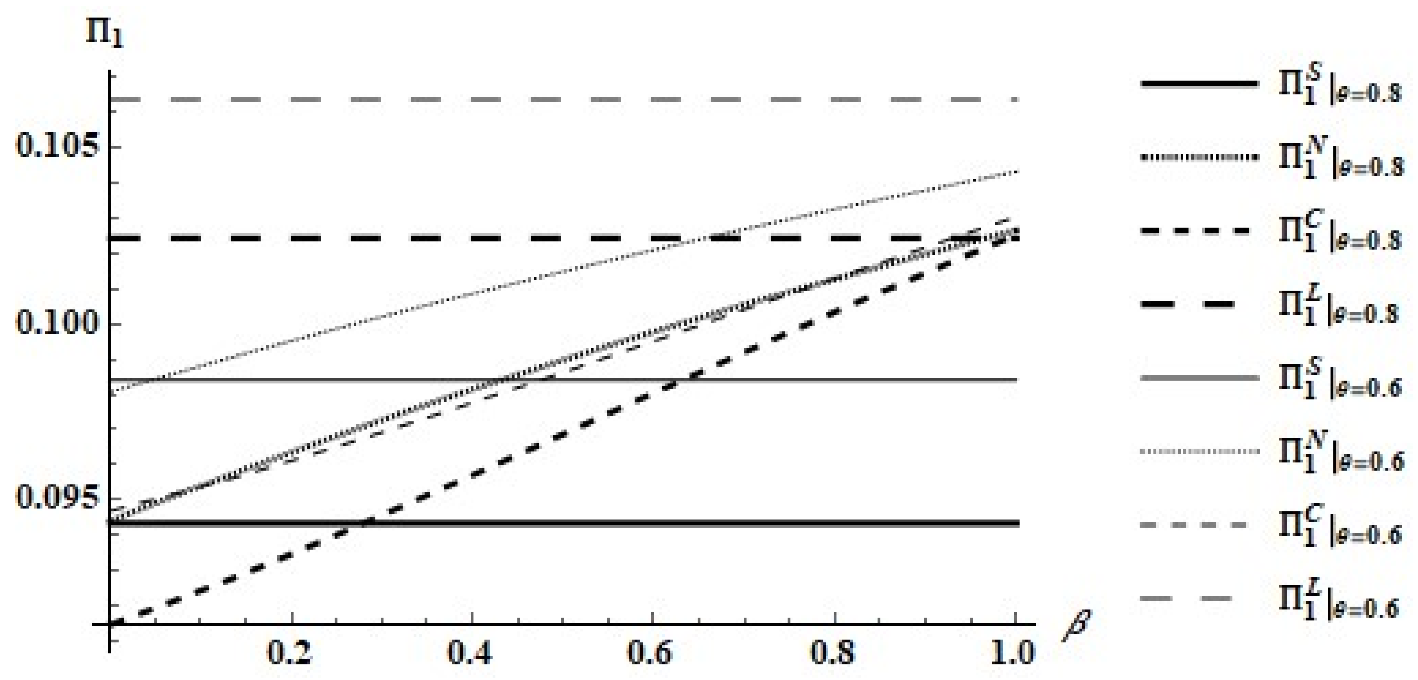
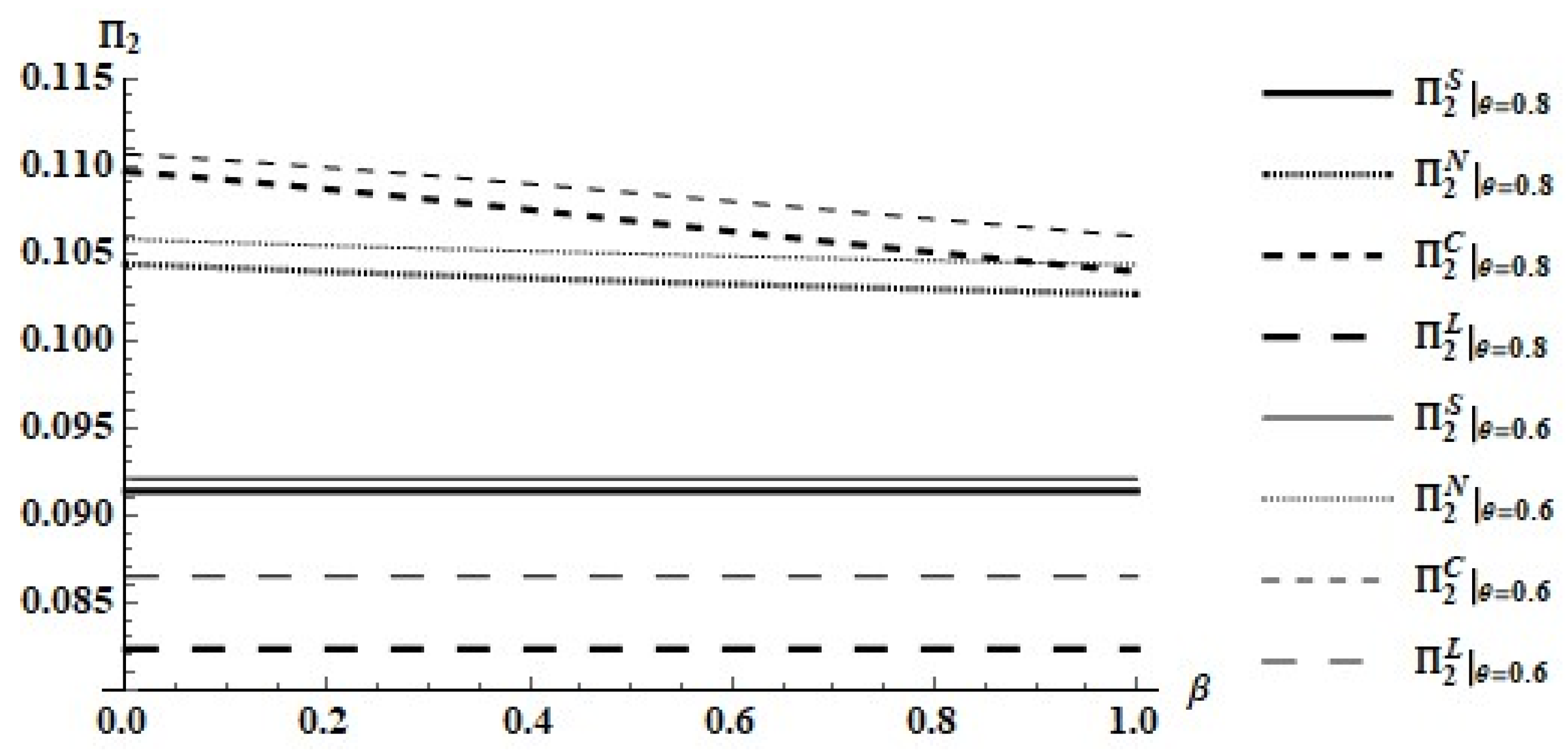
To derive some intuition for the results, let us consider the firms’ payoffs for two efficiency rates, and , as functions of . Figure 1 and Figure 2 show payoffs under the four possible scenarios.
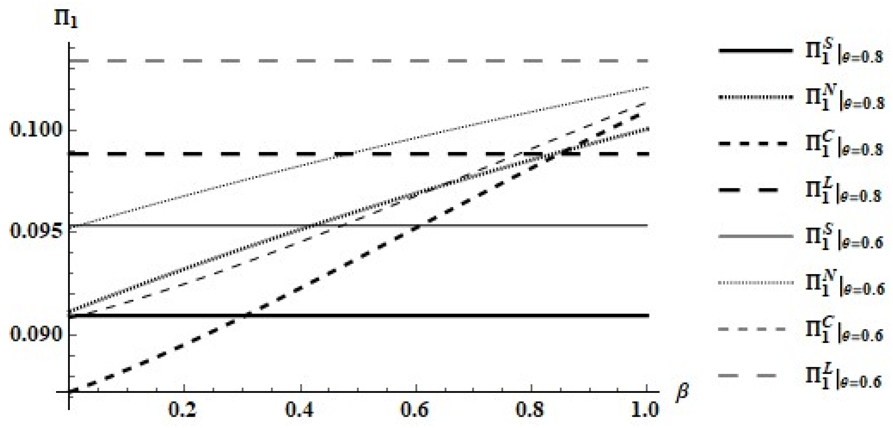
As Figure 1 reveals, for the foreign firm, the licensing agreement generally dominates all alternatives, and the non-cooperative RJV is generally second best. The non-cooperative (and the cooperative) dominates the licensing, when if . In addition, the status quo dominates the non-cooperative (and the cooperative) RJV for small spillover values () if . The status quo dominance is relative to the cooperative RJV increases as theta increases. The payoffs under the RJVs increase with the spillover rate that this firm enjoys.
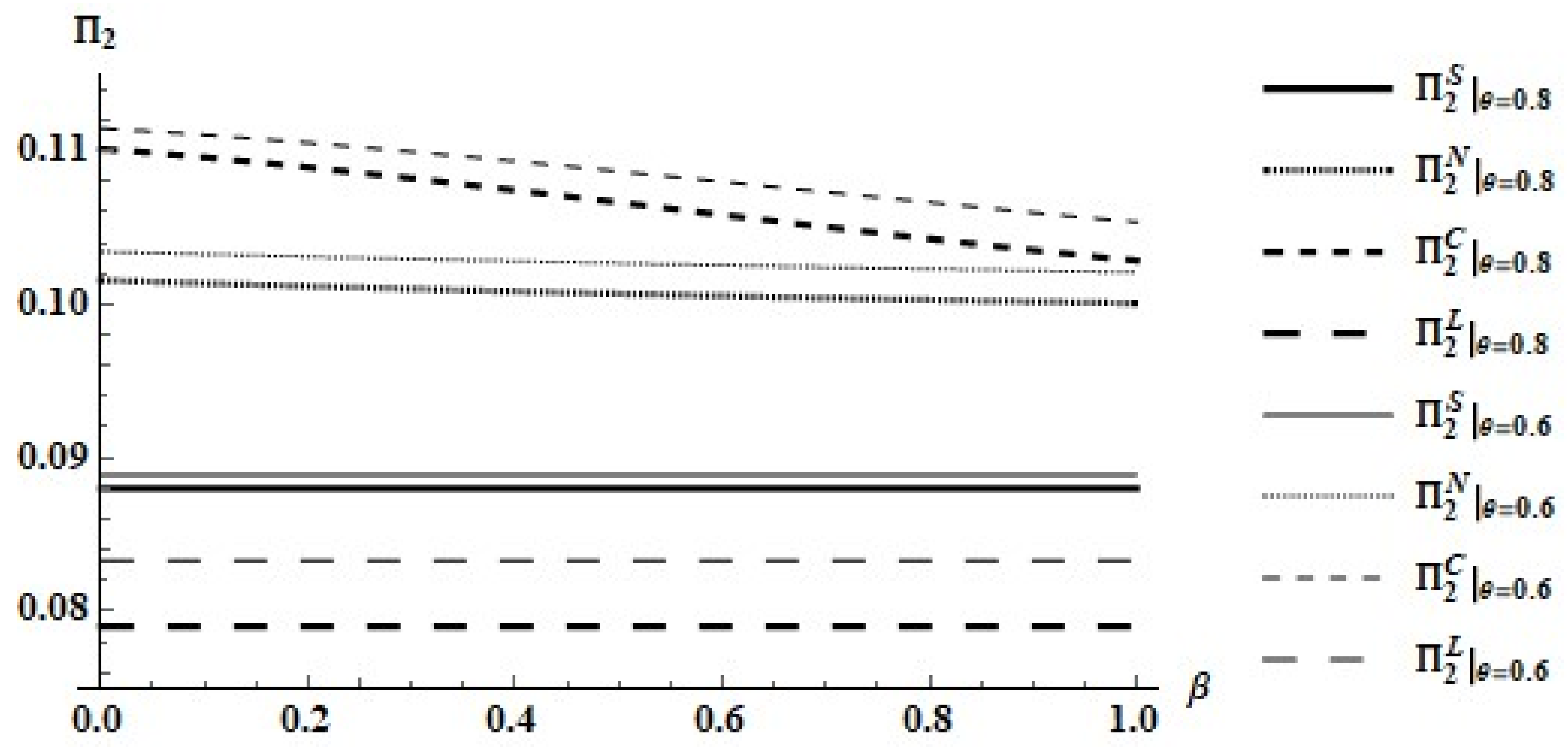
Figure 2 informs us that, for the domestic firm, cooperative RJV dominates non-cooperative RJV, both RJVs dominate the status quo, and the status quo dominates the licensing agreement. The payoffs under the RJVs decrease with the spillover rate enjoyed by the foreign firm, but they fall at a faster rate under the cooperative RJV.
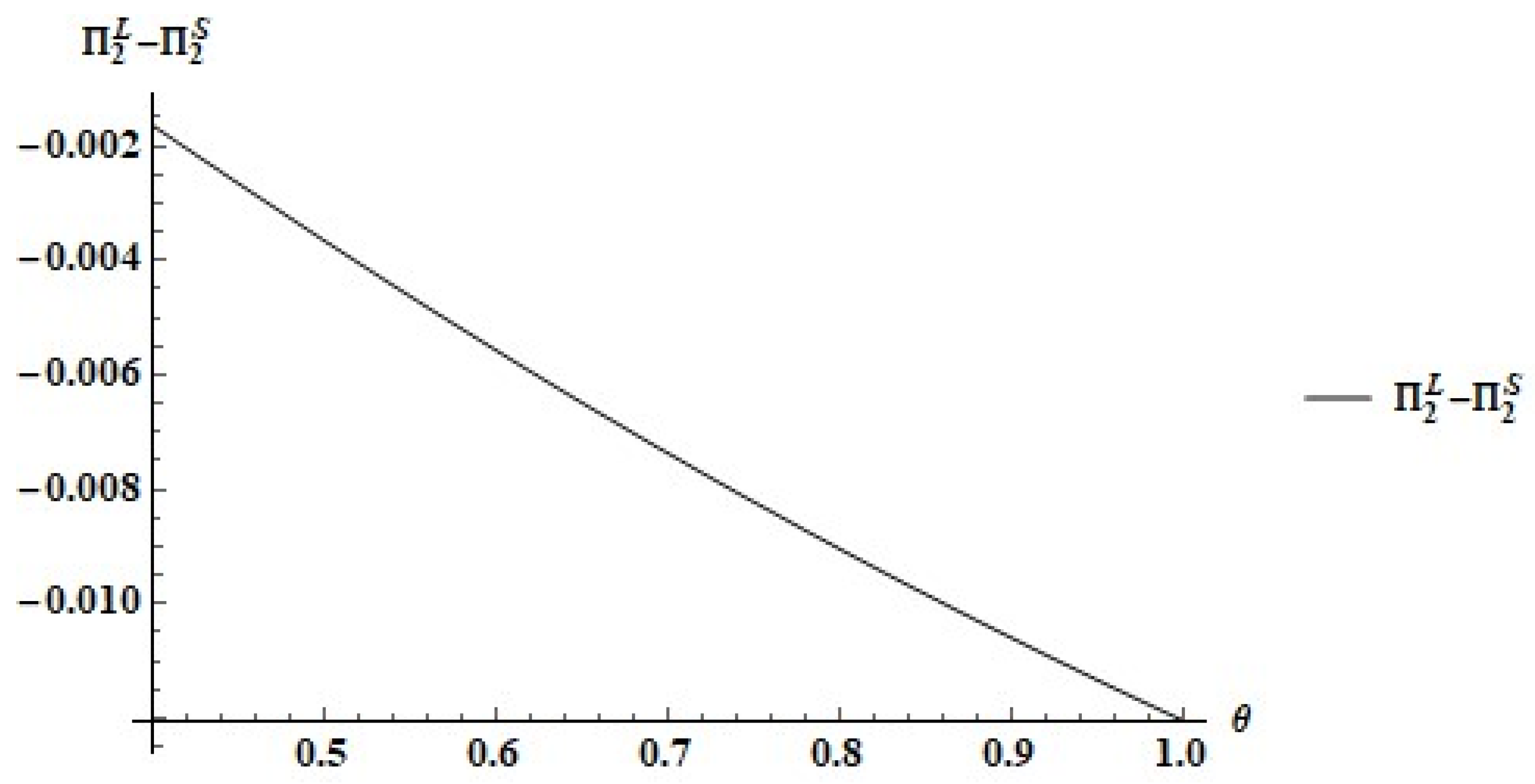
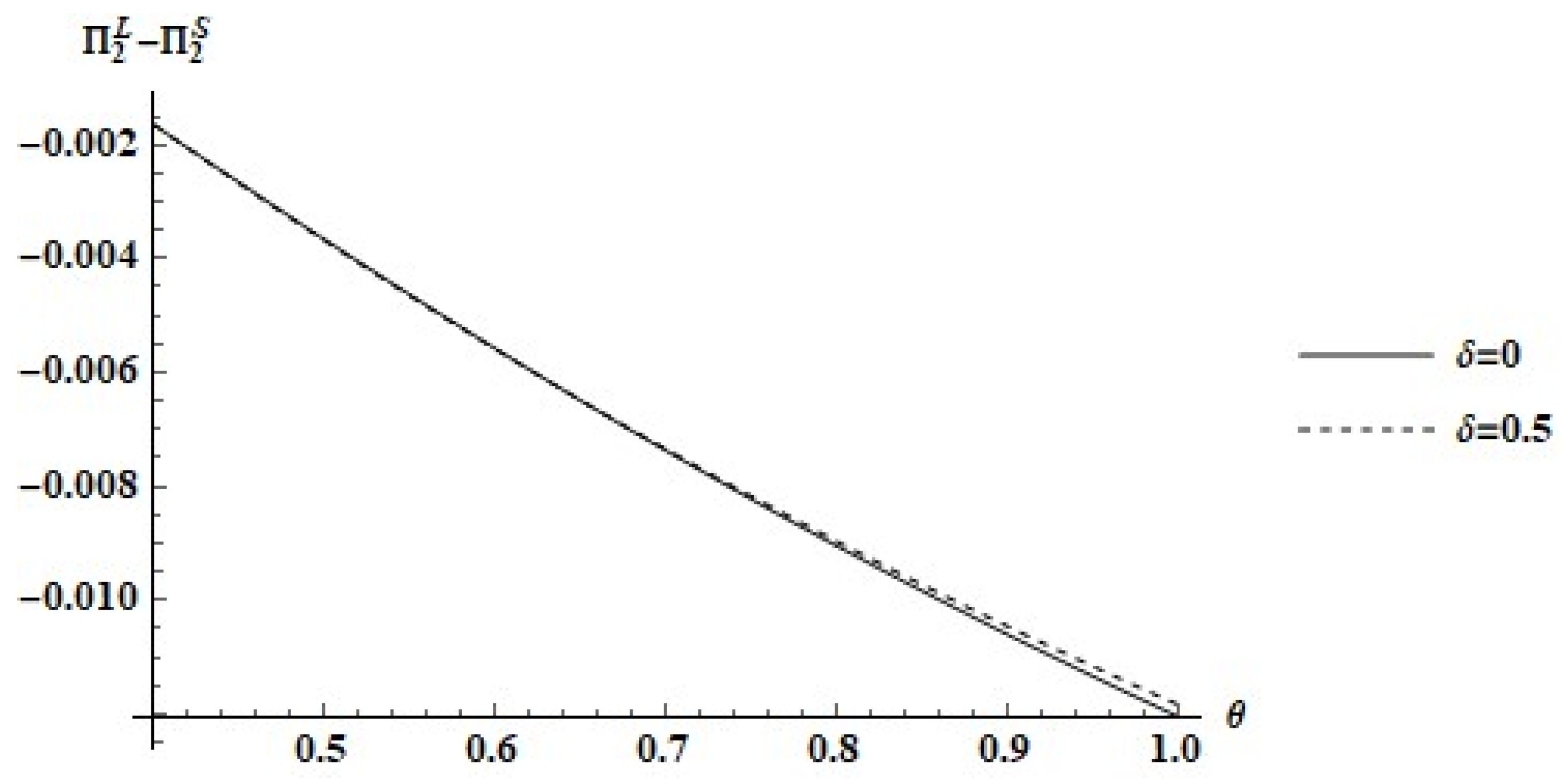
We now show that the licensing agreement is not implementable because it violates the participation constraint for the domestic firm. Figure 3 reveals that this firm’s profit in the status quo is higher than in the licensing agreement for .
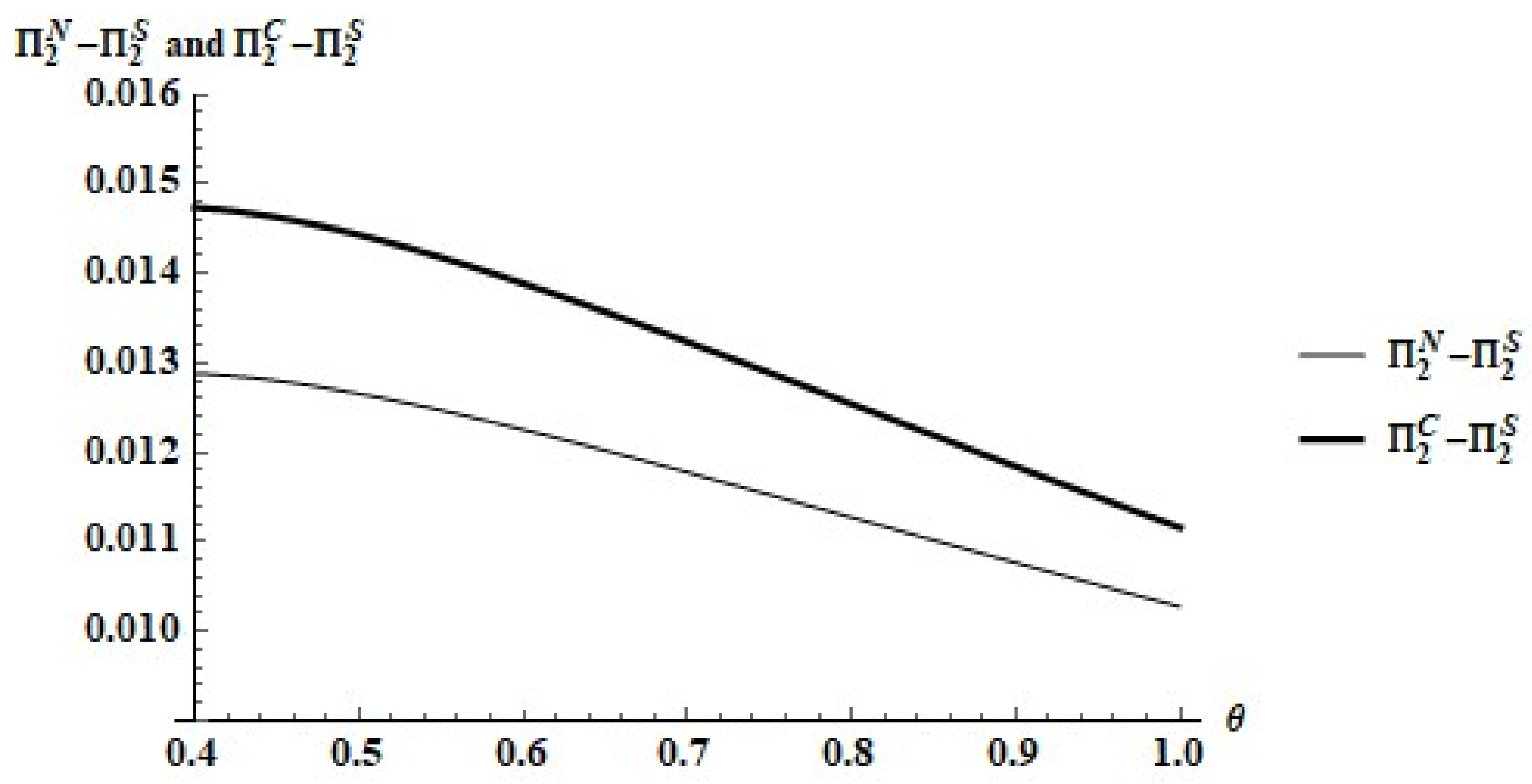
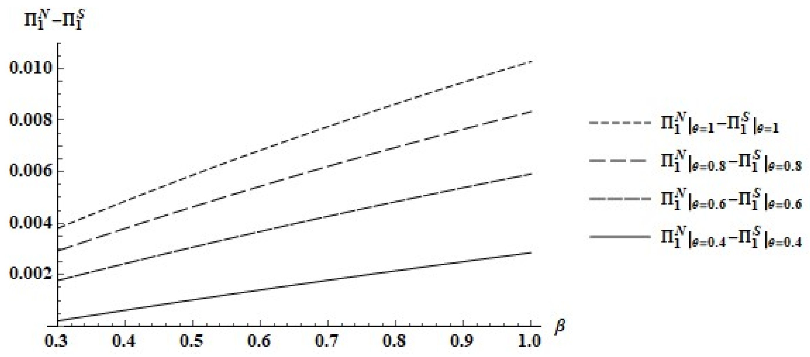
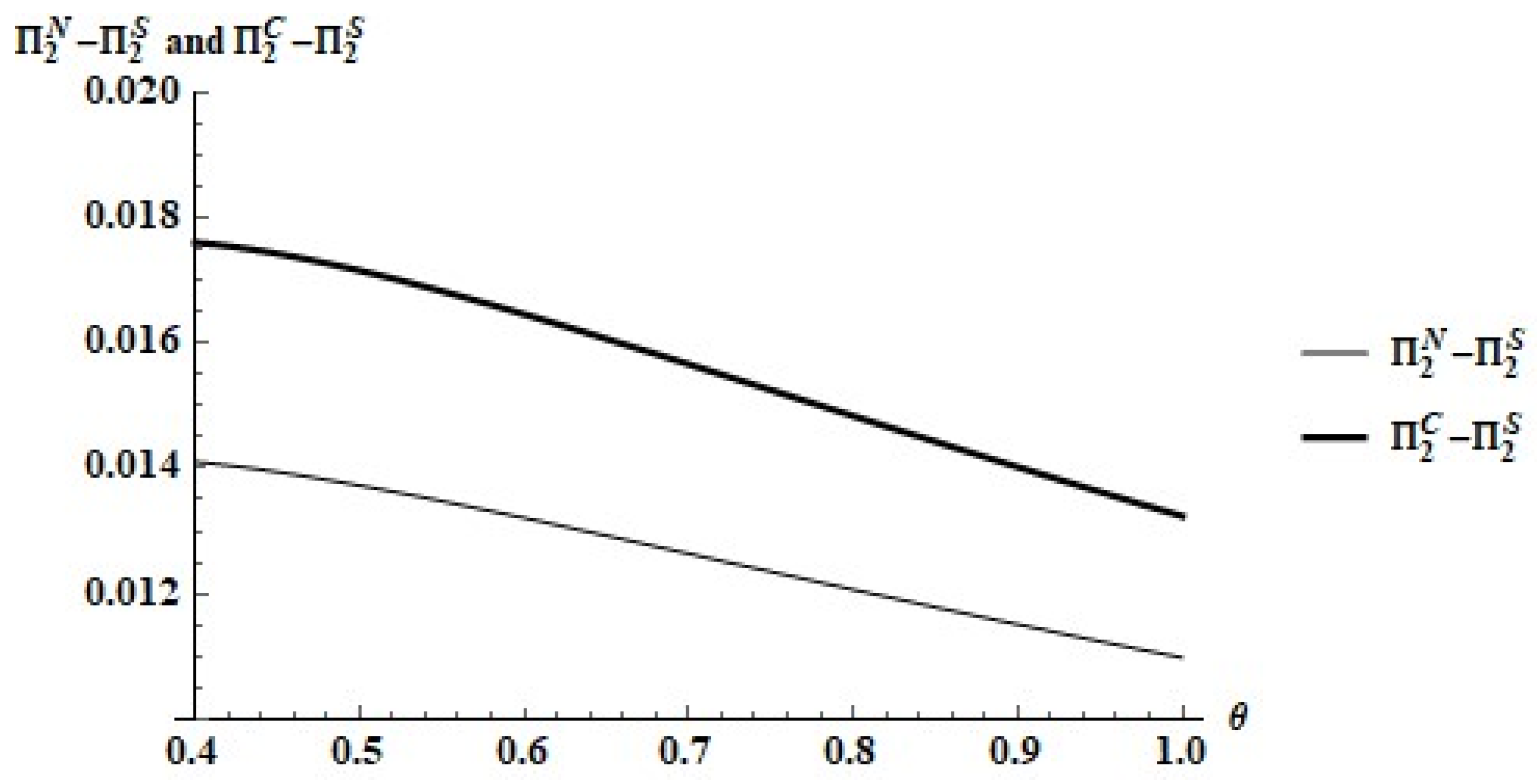
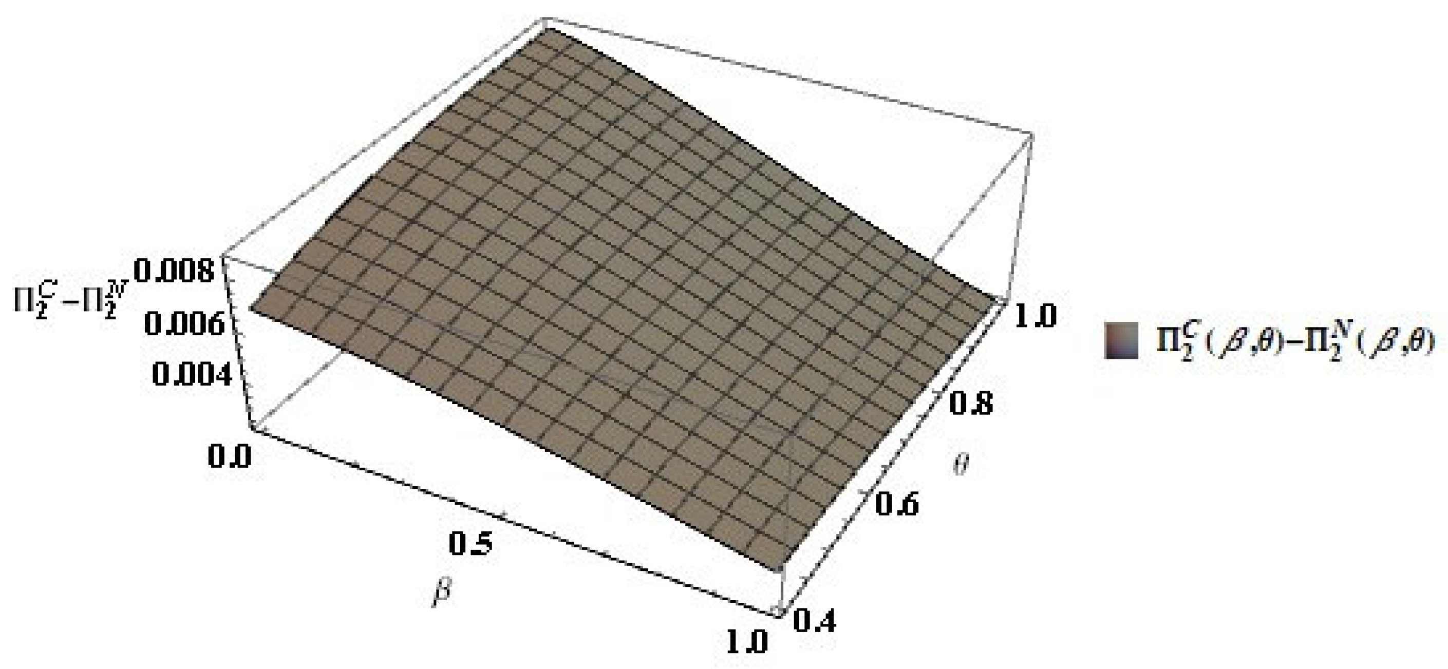
As it is apparent in Figure 2, the domestic firm always prefers either type of RJV to the status quo. Figure 4 compares the domestic firm’s payoffs under the RJVs to its payoff in the status quo when . These are the domestic firm’s lowest payoffs as functions of the parameters. Thus, the domestic firm prefers any RJV to the status quo. Figure 5 shows that, for the domestic firm, the cooperative RJV dominates the non-cooperative RJV for and .
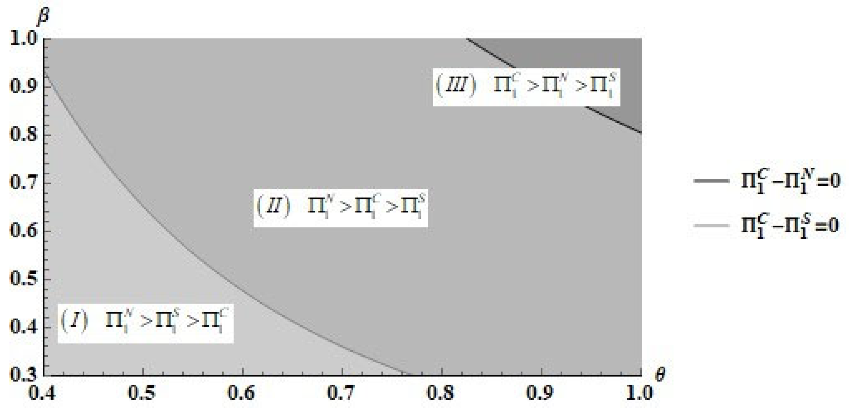
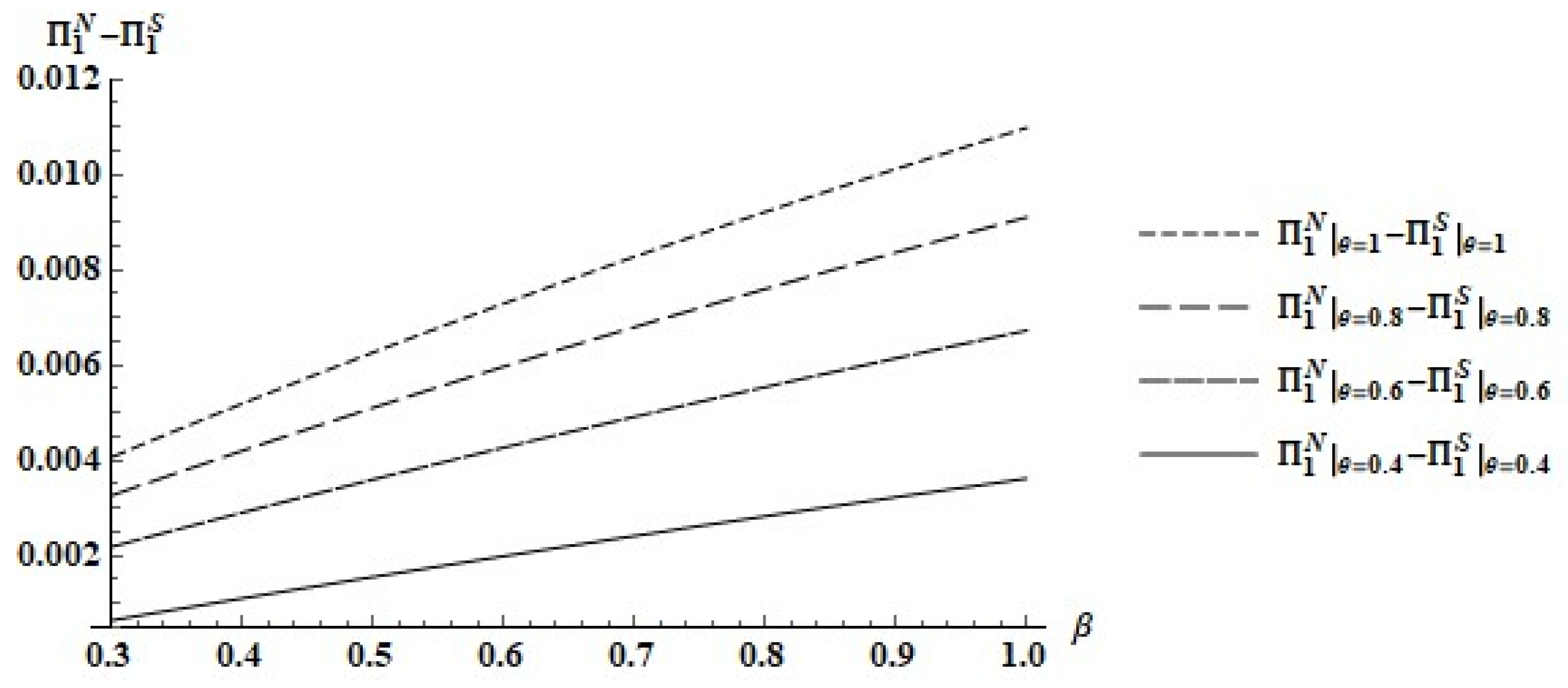
Let us now examine the foreign firm’s incentives to enter into an RJV with the domestic firm. As we pointed out above, the foreign firm prefers the status quo to either form of RJV if the efficiency and spillover parameters are sufficiently low. From Figure 1, it is apparent that the innovation premium that this firm obtains under each type of RJV (i.e., the difference between its payoff under each type of RJV and its payoff in the status quo) increases with both parameters’ values. Indeed, as Figure 6 reveals, if we restrict our analysis to parameter combinations that satisfy and , the innovation premium under the non-cooperative RJV is always positive.
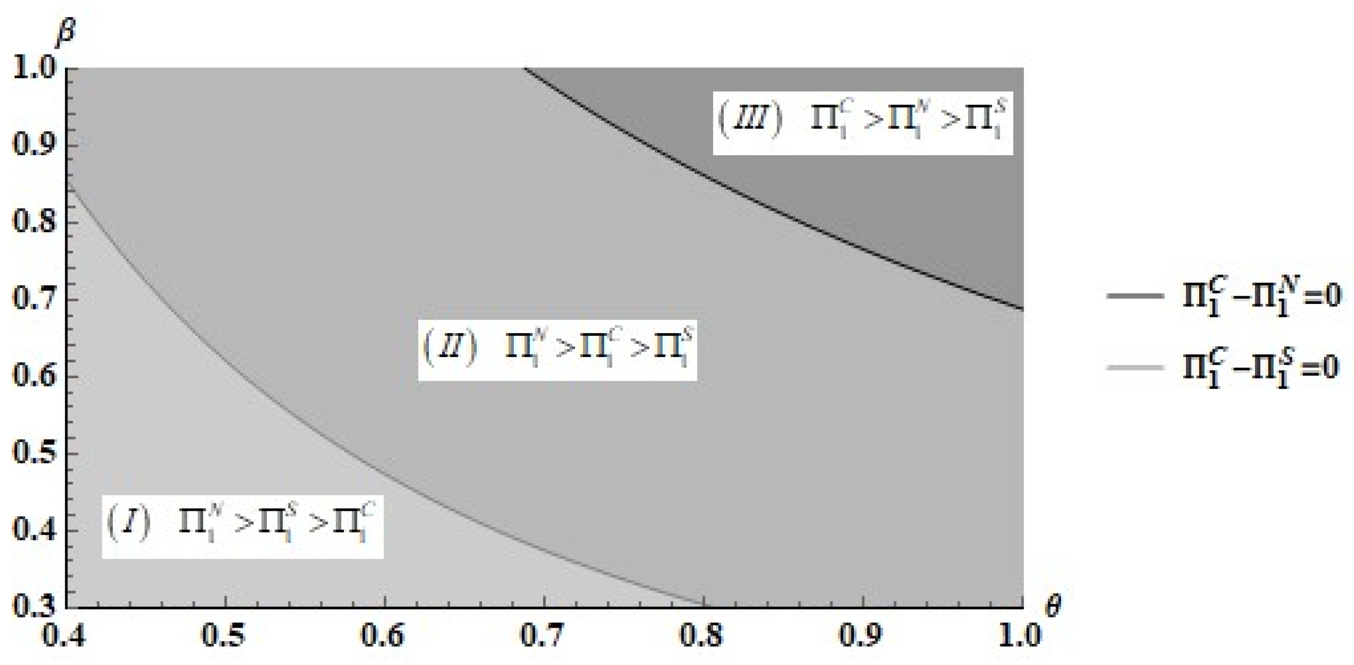
Given the results that Figure 1 and Figure 6 present, we now expect that, whenever both RJVs are feasible, the foreign firm prefers the non-cooperative RJV for most combinations of efficiency and spillover parameter values. In the relevant range, where both firms’ participation constraints are satisfied for at least one type of RJV, Figure 7 shows that the foreign firm rejects the cooperative RJV in an area with low values for the parameters. In addition, the foreign firm prefers the non-cooperative (cooperative) RJV in an area of intermediary (high) values for the parameters.
We summarize the outcomes in the first stage in the following proposition.
Proposition 2.
Suppose thatand. Then, for parameter values in
Proof.
Consider Figure 7. For parameters’ values in area I, the cooperative RJV is not feasible because it violates the foreign firm’s participation constraint. Hence, both firms select the feasible, non-cooperative RJV. For parameters’ values in areas II and III, both RJVs are feasible. In area II, the selection is random because the firms disagree about the top choice. In area III, the cooperative RJV dominates for both firms. Q.E.D. □
Henceforth, we assume that and . Together, these restrictions define the set of circumstances under which it is possible to implement an RJV. The more efficient the foreign firm is relative to the domestic firm, and the lower the spillover rate enjoyed by the foreign firm, the more likely it is that the outcome in the first stage is the non-cooperative RJV. The lower the asymmetry between the firms (both in terms of efficiency and spillover rates), the more likely it is that the outcome in the first stage is the cooperative RJV.
5. Domestic Competitiveness and Welfare
Having examined the circumstances under which each type of RJV is implementable, we now turn our attention to improvements in the competitiveness of the domestic firm and domestic welfare that the implementable RJVs may promote. We first consider the effects on domestic competitiveness.
The competitiveness of the domestic firm improves whenever innovation occurs. We are not able to capture such an improvement if we compare the firms in terms of their shares of the output market in the settings with innovation and without innovation. Since the firms produce the same output quantity in the subgame perfect equilibria (status quo, licensing, and RJVs), they have the same share of the output market. As both firms produce multiple products (abatement and output) and exert R&D efforts, one should compare their performances in terms of their shares of the industry’s profit. Since the firms face the same output price and the same price incentive to produce abatement (i.e., the pollution tax), a comparison of profit shares yields a precise competitiveness measure.
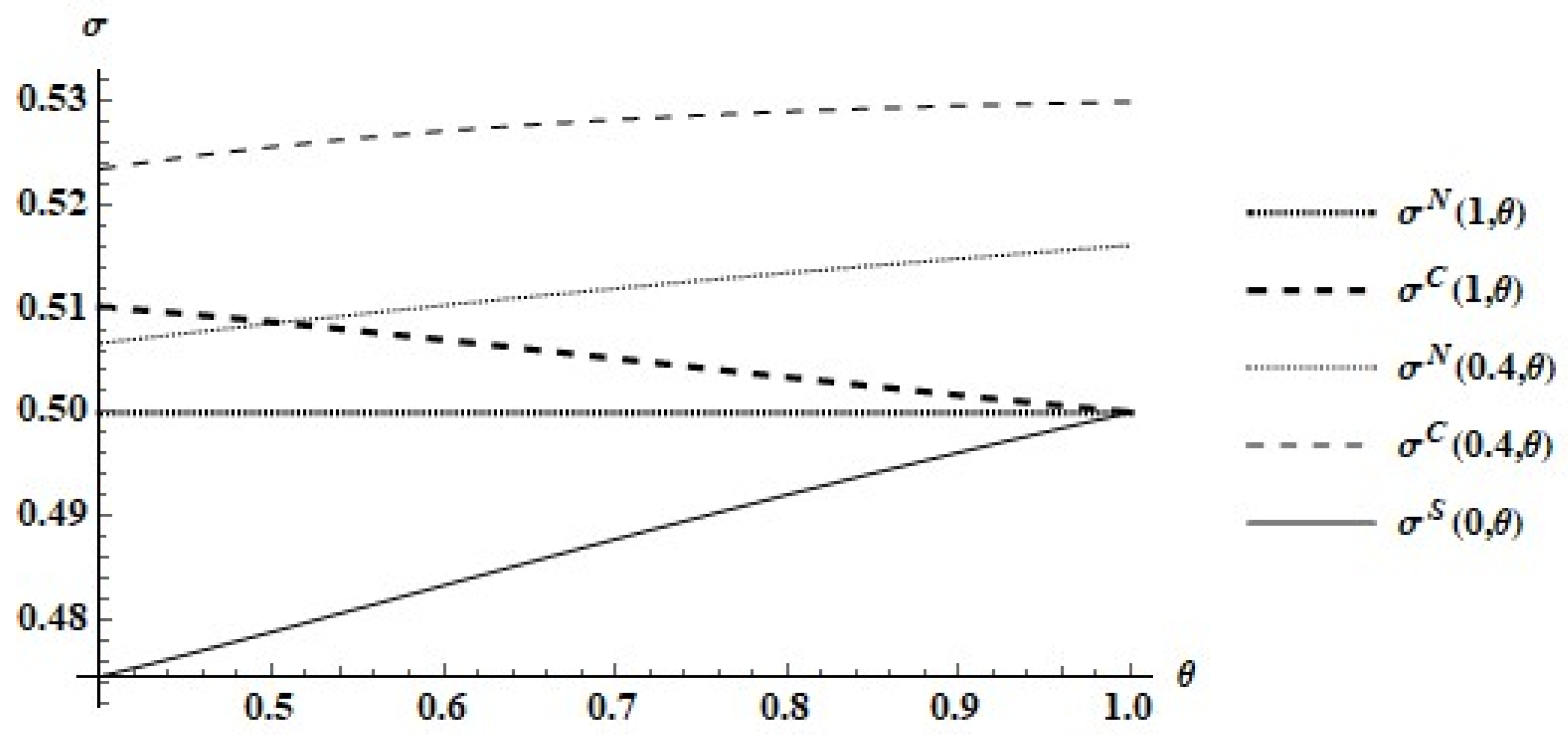
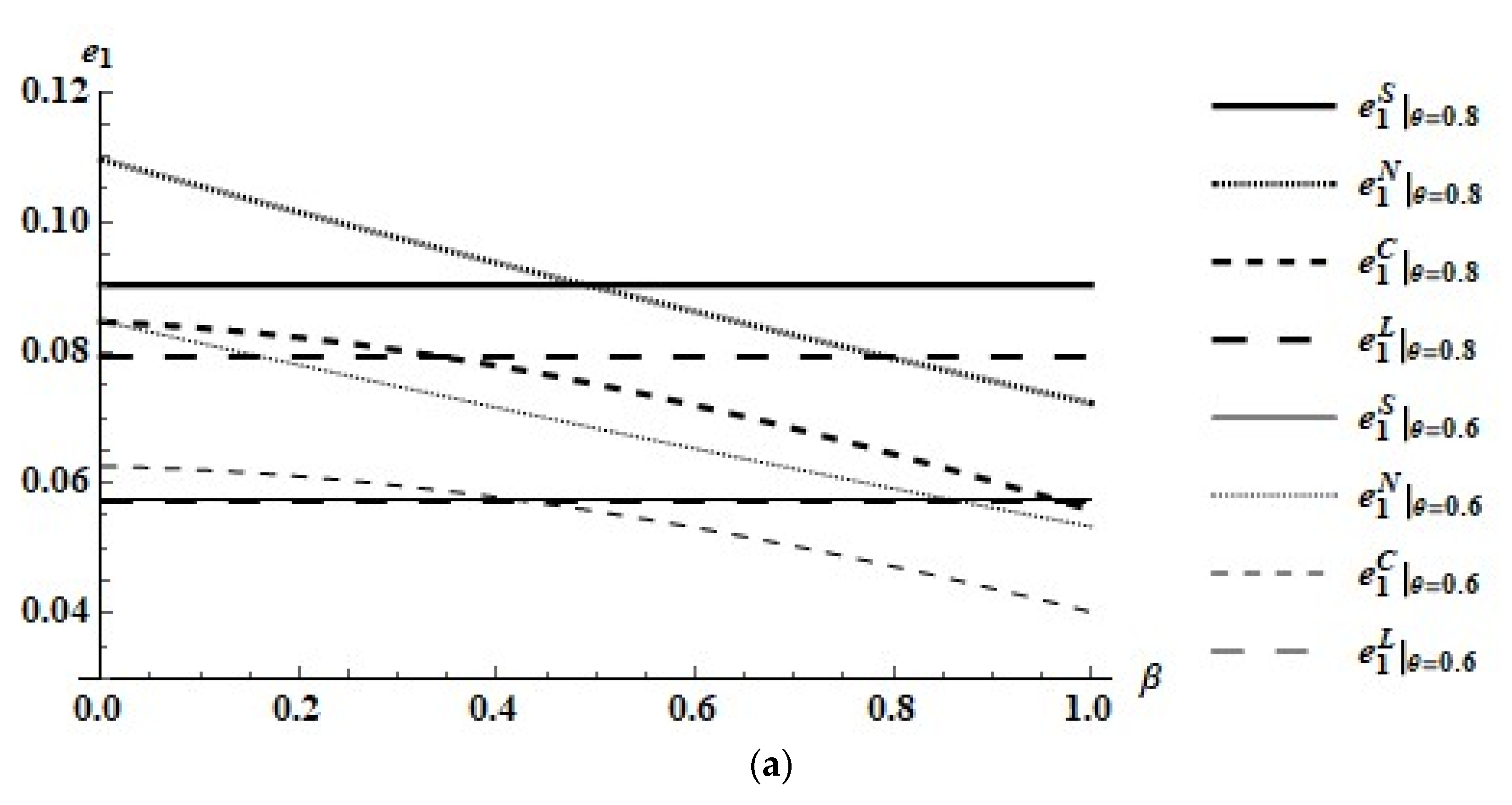
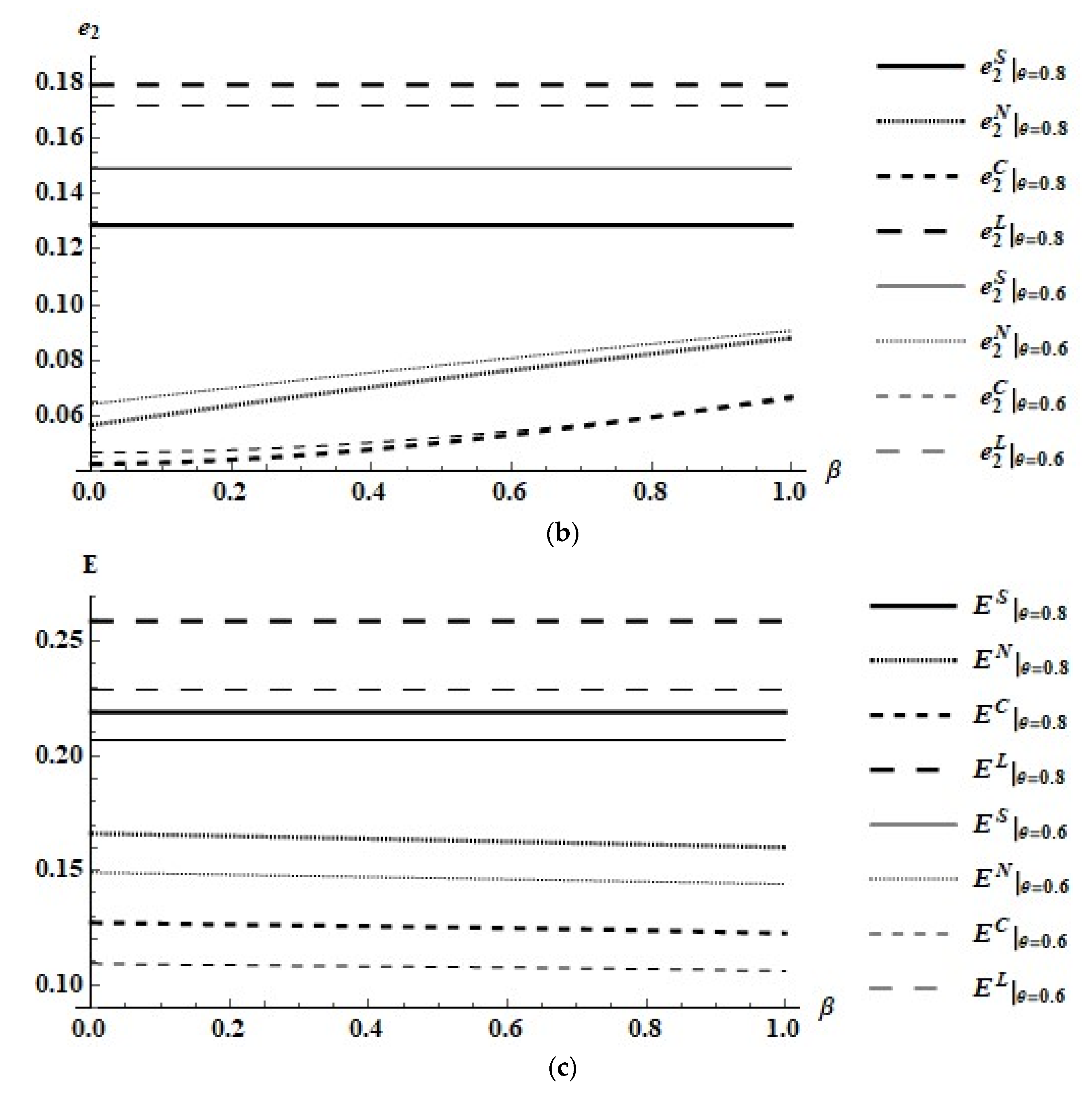
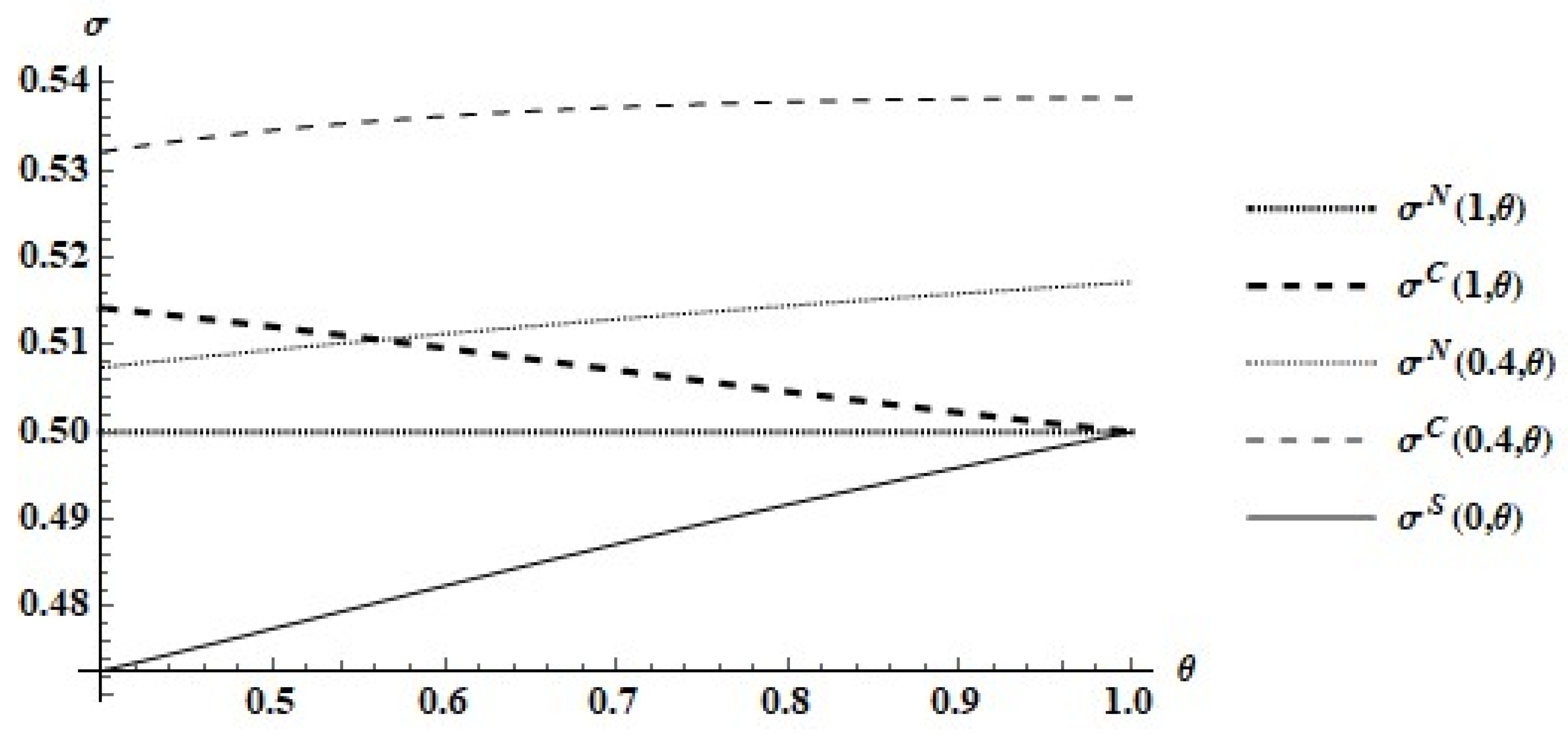
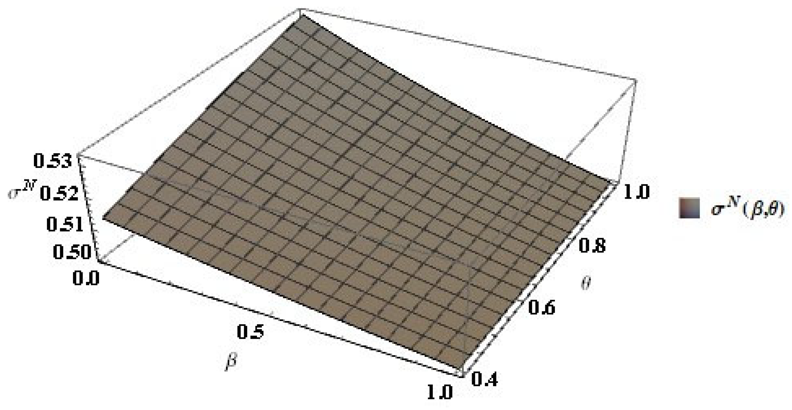
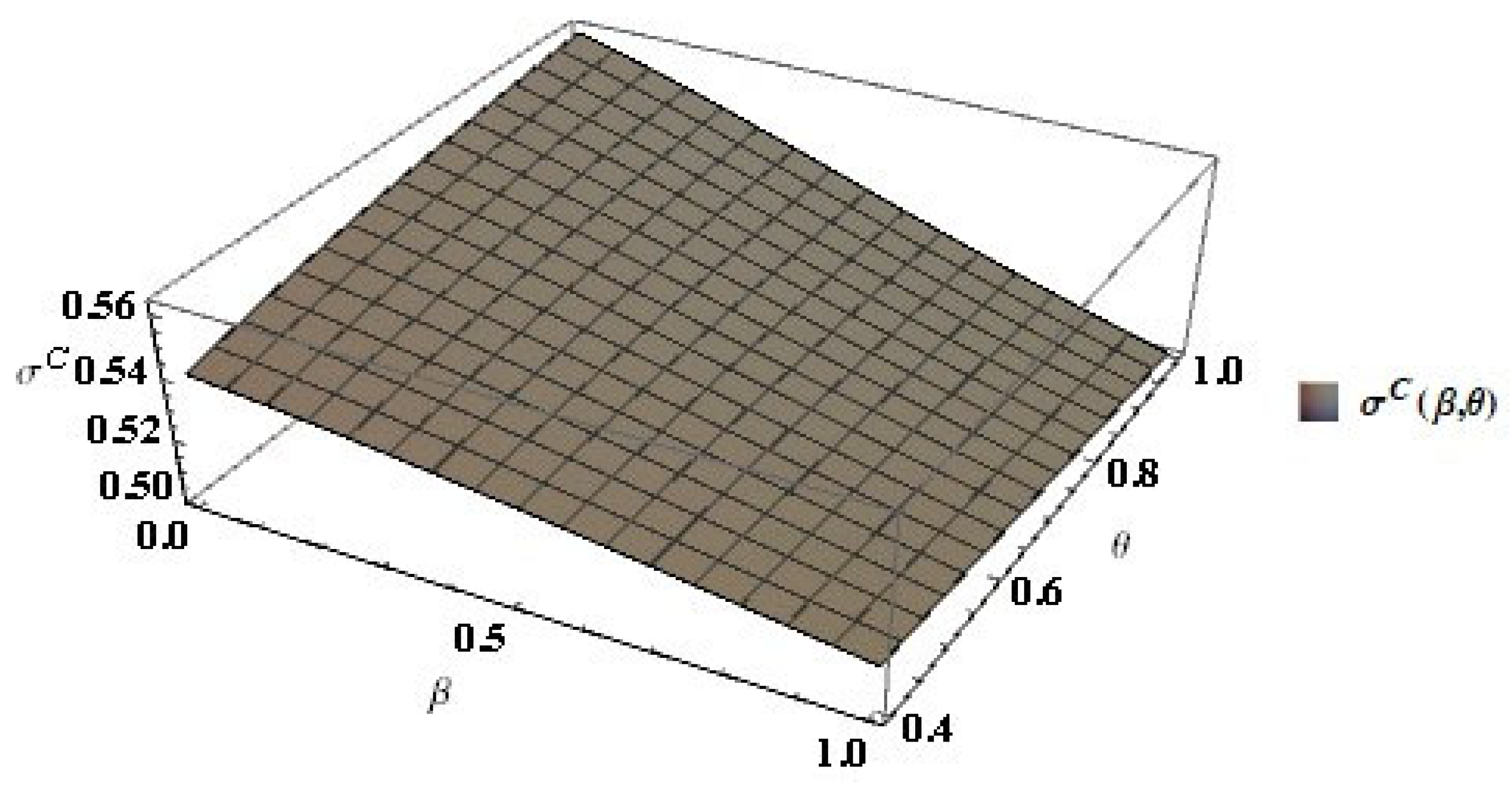
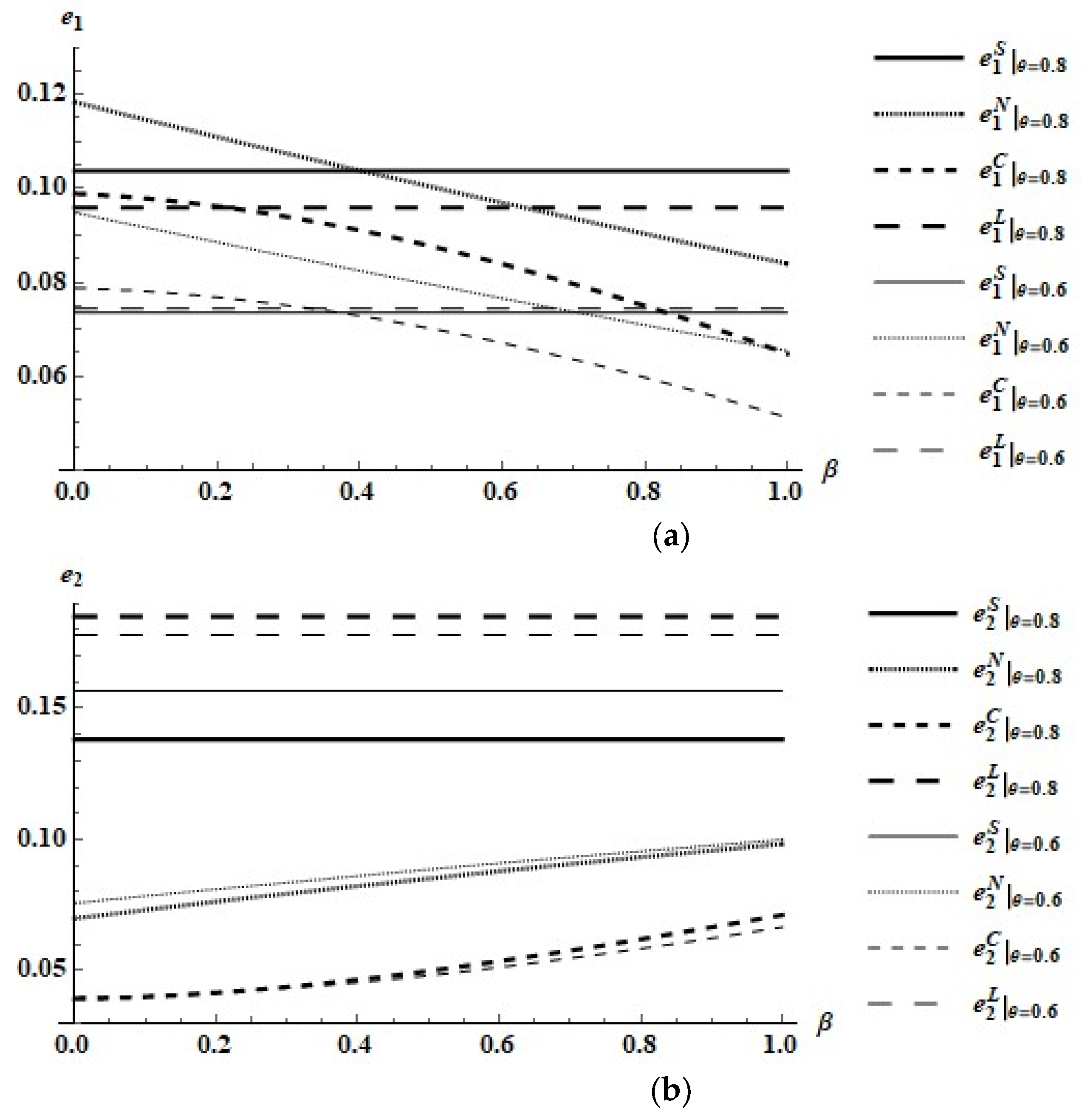
Let denote the domestic firm’s profit share as a function of the foreign firm’s spillover and efficiency rates, respectively. Figure 8 shows that the domestic firm’s profit share in the status quo increases as the technological gap decreases, and it equals half in the absence of a technological gap. Interestingly, we also see that the domestic firm’s profit share equals half despite the existence or not of a technological gap in the non-cooperative RJV if the firms are identical in terms of the R&D spillover rates (i.e., ). For a lower R&D spillover rate enjoyed by the foreign firm (), the domestic firm’s profit share in the non-cooperative RJV is always higher than the foreign firm’s share. In the cooperative RJV, the domestic firm’s profit share equals half only if there is no technological gap and both firms are identical in terms of R&D spillover rates. As the R&D spillover rate enjoyed by the foreign firm decreases from to , the domestic firm’s profit share in the cooperative RJV increases given the foreign firm’s efficiency rate, .
As Figure 2, Figure 4 and Figure 8 reveal for some particular efficiency and spillover rates, it appears that the greater the degrees of asymmetry between the firms (in terms of efficiency and spillover rates), the greater the domestic firm’s relative benefit from engaging in an RJV. Figure 9 and Figure 10 confirm this intuition for and .
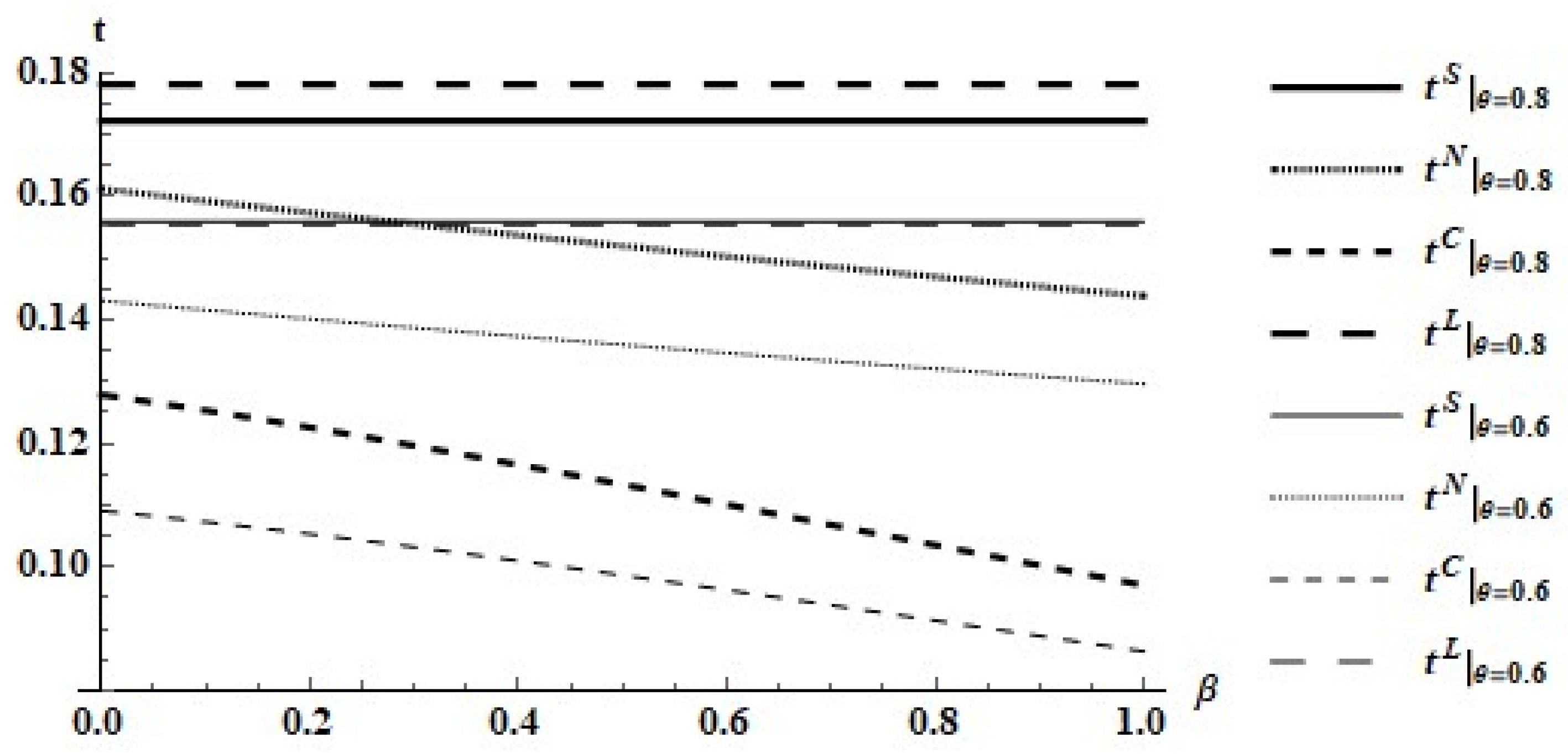
Relative to the status quo, a feasible RJV yields an increase in the domestic firm’s profit share because the R&D spillovers enable the domestic firm to reduce its environmental regulatory cost. The cost savings produced by the innovation would occur even if the firm faced the same pollution tax in both scenarios. However, the costs savings are more substantial because the government’s optimal response to the implementation of an innovation agreement is to reduce the pollution tax, as Figure 11 reveals.
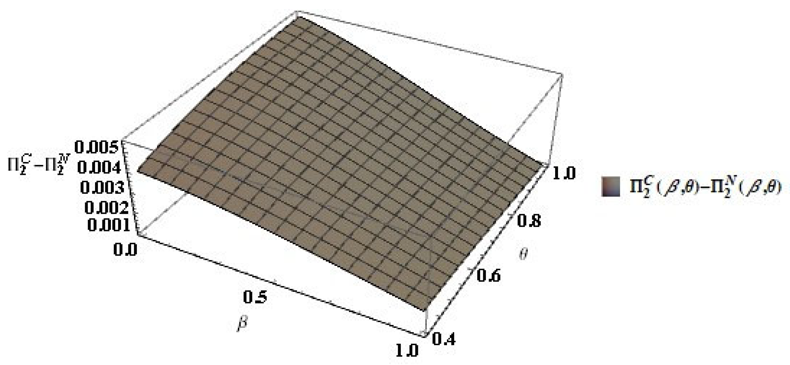
One may worry that the lower pollution tax is associated with a higher amount of pollution. However, consistent with the previous argument that an implementable RJV improves environmental performance, we see in Figure 12c that pollution levels under the RJVs are lower than in the status quo and in the licensing agreement.
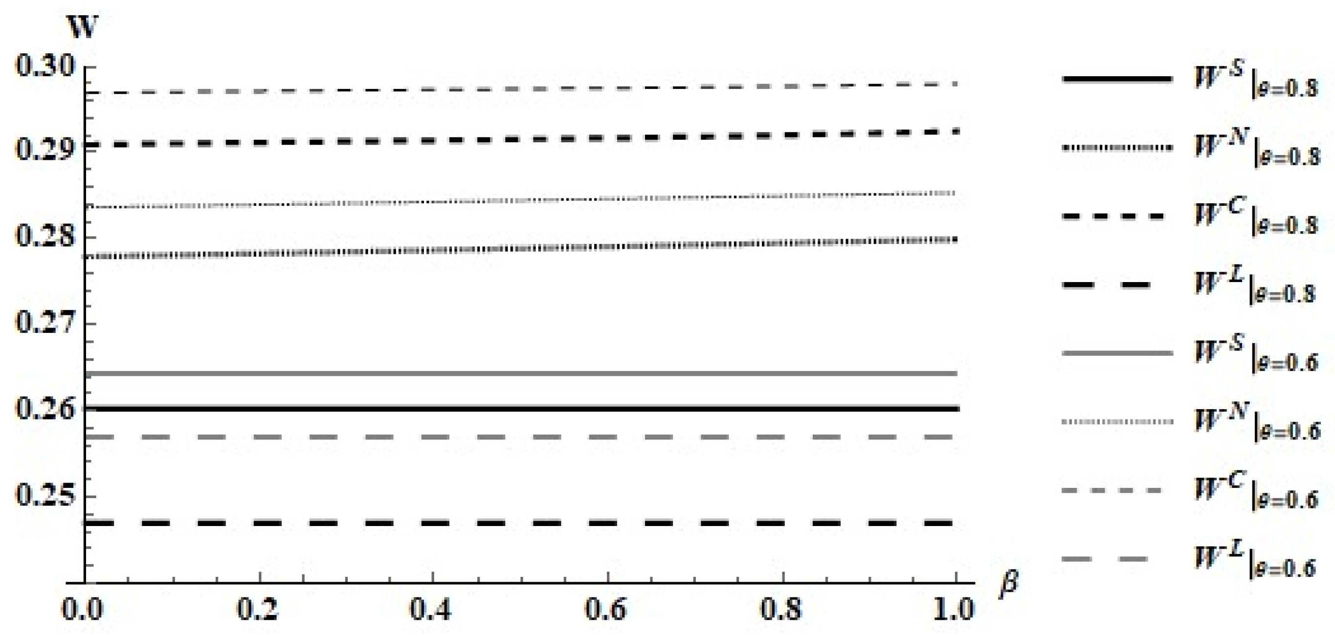
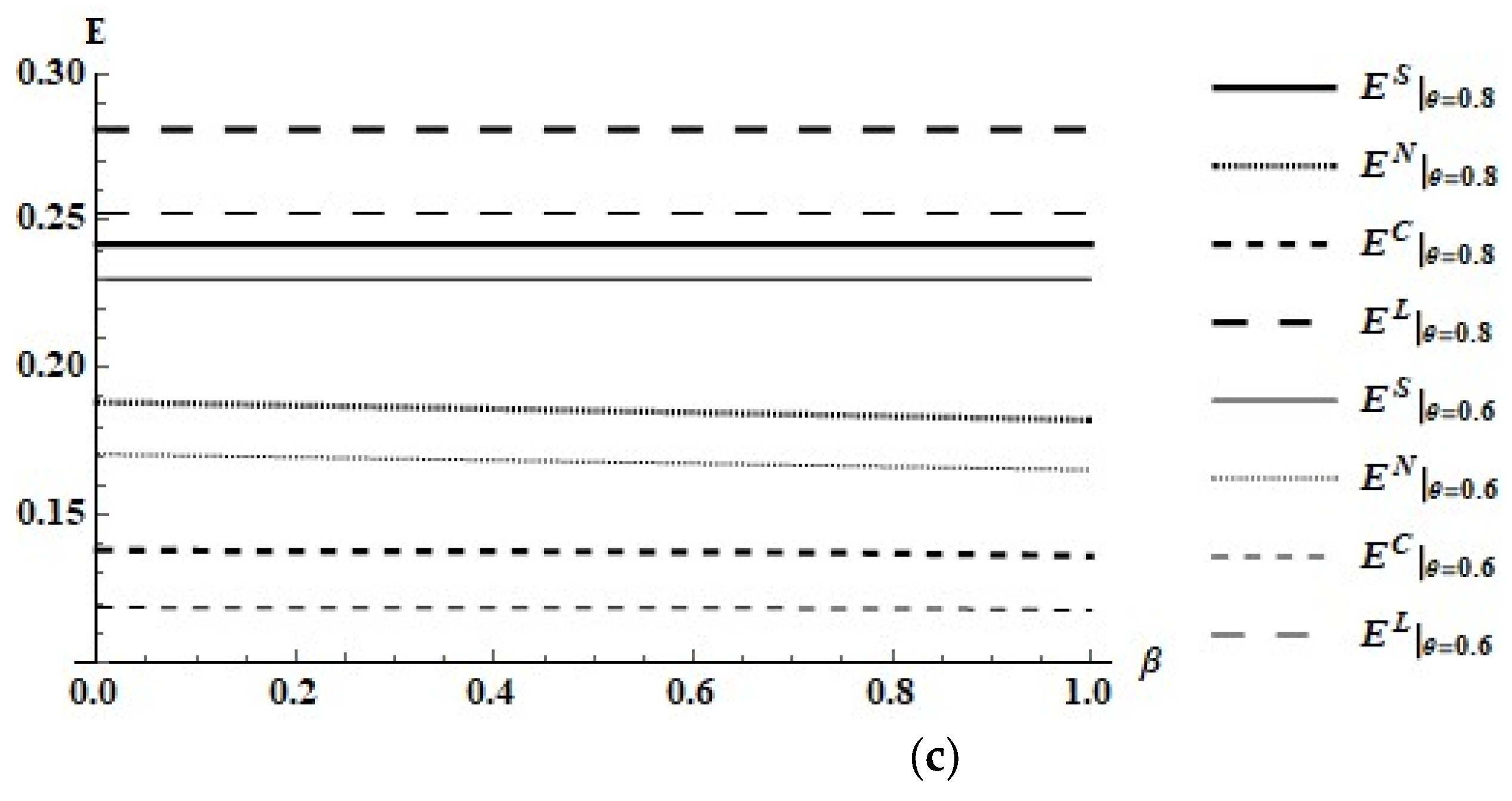
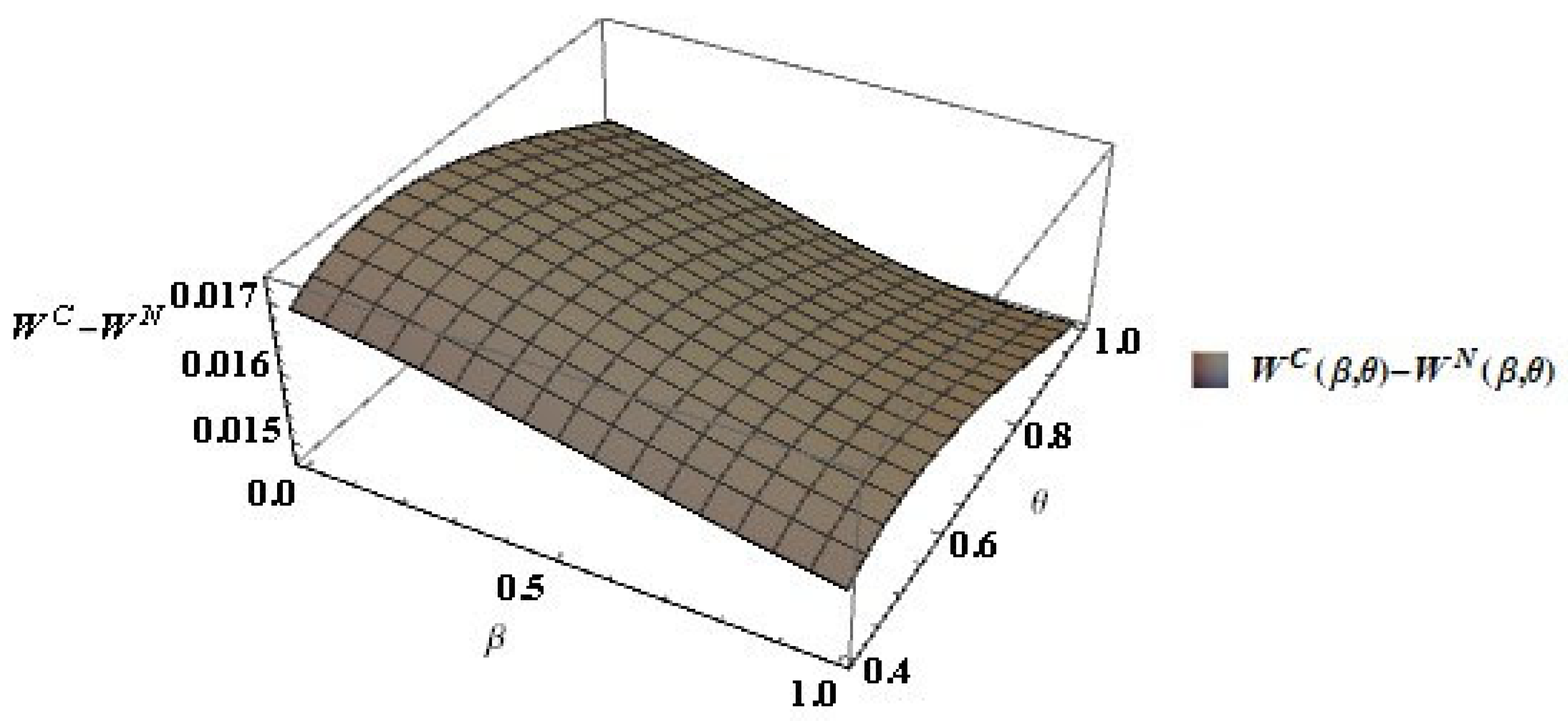
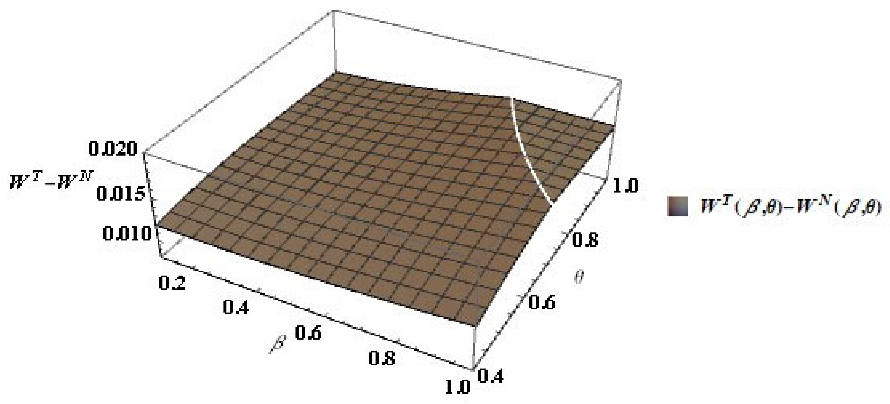
Let us now examine the welfare effects. It is straightforward to show that the settings with RJVs are dominant in terms of welfare. As before, for illustration purposes, we plot welfare as a function of for two efficiency rates, . Figure 13 shows that, in each case, welfare is highest under the cooperative RJV, second best under the non-cooperative RJV, and lowest under licensing. Fortunately, the licensing agreement is not implementable. Figure 14 shows that the cooperative RJV dominates the non-cooperative RJV not only in the particular cases examined in Figure 13, but in general.
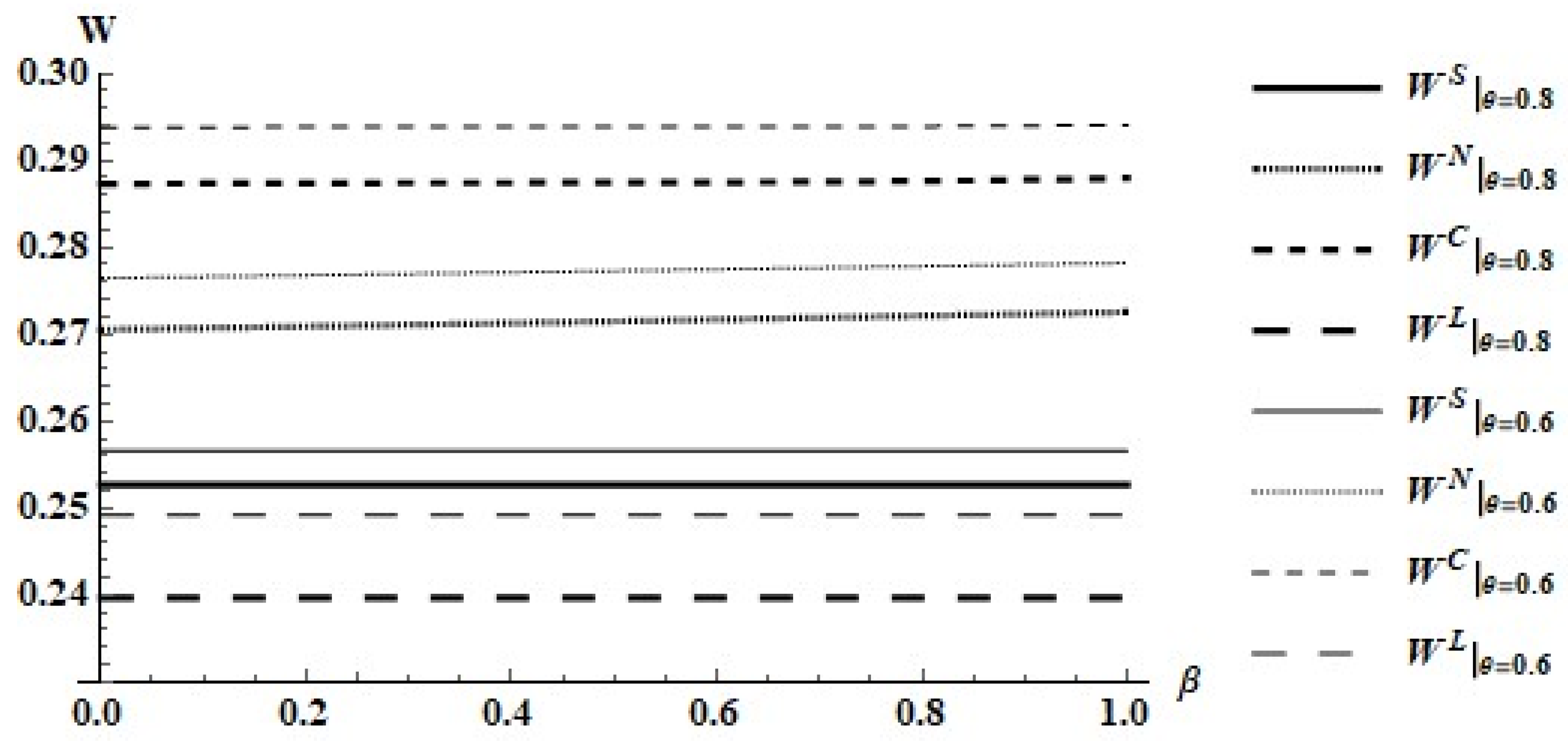
Since the cooperative RJV dominates the non-cooperative RJV in terms of welfare, a potential welfare improving policy that the government may undertake is to “bribe” the foreign firm to select a feasible cooperative RJV whenever it strictly prefers a feasible non-cooperative RJV. Remember that this occurs in areas I and II of Figure 7. Let for all and such that denote the lump-sum transfer payment (subsidy) that the government makes to the foreign firm to induce it to accept the cooperative RJV when it prefers the non-cooperative RJV. Assume that if . Let and denote the welfare levels under the non-cooperative RJV and under the cooperative RJV net of the subsidy , respectively. Figure 15 shows that such a subsidy policy is, indeed, welfare improving because for and .
6. A Robustness Exercise
The reader may wonder if our comparative results are sensitive to our assumption that the cost function is separable in abatement net of R&D and R&D. To demonstrate that the results do not appear to depend on the simple, separable, cost function, we relax the assumption that the cost function is separable by assuming that there are diseconomies of scope in abatement net of R&D and R&D activities. Let . We compare Figure 1, Figure 2, Figure 3, Figure 4, Figure 5, Figure 6, Figure 7, Figure 8, Figure 9, Figure 10, Figure 11, Figure 12, Figure 13, Figure 14 and Figure 15 in Section 4.4 with Figure 16, Figure 17, Figure 18, Figure 19, Figure 20, Figure 21, Figure 22, Figure 23, Figure 24, Figure 25, Figure 26, Figure 27, Figure 28, Figure 29 and Figure 30 below.
In Figure 16, for the foreign firm, the licensing agreement dominates all alternatives, and the non-cooperative RJV is second best for . The cooperative and non- cooperative RJVs dominate licensing, when if . Figure 1 and Figure 16 show that the foreign firm is likely to prefer RJVs to licensing in the presence of diseconomies of scope in abatement net of R&D and R&D activities.
Figure 17 informs us that, for the domestic firm, cooperative RJV dominates non-cooperative RJV, both RJVs dominate the status quo, and the status quo dominates the licensing agreement.
In Figure 18, the licensing agreement is not implementable because it violates the participation constraint for the domestic firm. Figure 18 reveals that this firm’s profit in the status quo is higher than in the licensing agreement for both in the case of a separable cost function and in the case of a non-separable cost function.
Figure 19 compares the domestic firm’s payoffs under the RJVs to its payoff in the status quo when . The domestic firm prefers any RJV to the status quo.
Figure 5 and Figure 20 show that, for the domestic firm, the cooperative RJV dominates the non-cooperative RJV for and with separable and non-separable cost functions.
Similar to Figure 6 when the cost function is separable, Figure 21 shows that the foreign firm prefers the non-cooperative RJV to the status-quo when the cost function is non-separable.
Figure 22 is similar to Figure 7: the foreign firm also prefers the non-cooperative (cooperative) RJV in an area of intermediary (high) values for the parameters when the cost function is non-separable.
Figure 8 and Figure 23 show that the domestic firm’s profit share in the status quo increases as the technological gap decreases, and it equals half in the absence of a technological gap. The domestic firm’s profit share equals half despite the existence or not of a technological gap in the non-cooperative RJV if . In the cooperative RJV, the domestic firm’s profit share equals half only if there is no technological gap and both firms are identical in terms of R&D spillover rates. As the R&D spillover rate enjoyed by the foreign firm decreases, the domestic firm’s profit share in the cooperative RJV increases, given the foreign firm’s efficiency rate, .
Similar to Figure 9 and Figure 10, Figure 24 and Figure 25 confirm the fact that the greater the degrees of asymmetry between the firms (in terms of efficiency and spillover rates), the greater the domestic firm’s relative benefit from engaging in an RJV both in a case of separable cost function and in the case of a non-separable cost function.
Comparing Figure 11 and Figure 26, we see identical results with respect to the pollution tax rate: it is lowest under a cooperative RJV and the second lowest under a non-cooperative RJV. The tax rate under the status quo is highest for with the non-separable cost function.
As in Figure 12c, Figure 27c informs us that the pollution levels under the RJVs are also lower than in the status quo and in the licensing agreement with a non-separable cost function.
Figure 13 and Figure 28 show that, in each case, welfare is highest under the cooperative RJV, second best under the non-cooperative RJV, and lowest under licensing. Figure 14 and Figure 29 show that the cooperative RJV dominates the non-cooperative RJV not only in the particular cases examined in Figure 13 and Figure 28, but in general.
Figure 15 and Figure 30 show that such a subsidy policy is, indeed, welfare improving because for and with separable and non-separable cost functions.
In sum, we find that the qualitative results do not seem to depend on the assumption that the cost function is separable. Both forms of RJV are likely to be implementable if there are diseconomies of scope in the abatement net of R&D and R&D.
7. Conclusions
RJVs and licensing are common innovation agreements. These agreements occur in many nations, developed and developing, and, in several instances, they feature the participation of international firms. A substantial share of such agreements derives their motivation from attempts of their participants to improve their environmental performances. There is evidence that, in some cases, the firms that form RJVs display forward-looking behavior with respect to the occurrence of new (or more stringent) environmental regulations.
This paper examines the potential formation of RJVs when, imperfectly competitive, asymmetric firms anticipate the effects that the interaction between each of the three different forms of innovation agreements and environmental regulation produced. The duopoly contains domestic and foreign firms. The regulator (domestic government) cares about domestic welfare, which ignores the producer surplus that the foreign firm enjoys.
We obtain several important results. First, we show that licensing is not implementable because it makes the domestic firm worse off relative to the status quo. Second, we demonstrate that both forms of RJVs are implementable: the non-cooperative RJV is more likely the greater the degrees of asymmetries (in terms of efficiency and R&D spillover rates) between the firms, while the cooperative RJV is more likely the lower the degrees of asymmetries. Third, we find that the implementation of both RJVs improves the domestic firm’s competitiveness and domestic welfare. Welfare improvements are larger under the cooperative RJV. Finally, we show that a subsidy policy that induces the foreign firm to accept the cooperative RJV when it strictly prefers the non-cooperative RJV is welfare improving.
An interesting avenue for future research is to analyze the circumstances under which the double dividend hypothesis holds in a similar setting. For example, one can assume that the domestic government regulates the industries by levying an emission tax to control pollution while also regulating the foreign firm by levying a tariff on its output to protect the domestic firm. Providing the government with the additional policy instrument (i.e., the tariff) would enrich the analysis and may lead to a different set of policy implications relative to those that we advance in this paper. Nevertheless, we anticipate that the incentives to form RJVs would remain strong in this richer environment.
Author Contributions
Conceptualization: N.A. and E.C.D.S.; methodology: N.A. and E.C.D.S.; formal analysis: N.A. and E.C.D.S.; writing—original draft preparation: N.A. and E.C.D.S.; writing—review and editing: N.A. and E.C.D.S. All authors have read and agreed to the published version of the manuscript.
Funding
This research was supported by Japan Society for the Promotion of Science KAKENHI grant number 25780166.
Institutional Review Board Statement
Not applicable.
Informed Consent Statement
Not applicable.
Data Availability Statement
Not applicable.
Conflicts of Interest
The authors declare no conflict of interest.
Appendix A
We provide the proofs for Proposition 1 in Appendix A. In all equilibria, for and .
Proof of Proposition 1.
Equation (4) implies that . Then, because . Equation (3) imply because and is increasing at an increasing rate in and separable in and . Hence, . Combining with Equation (5) yields , which implies because is increasing at an increasing rate in and separable in and . Then, and imply . Q.E.D. □
Appendix B
In Appendix B, we show the conditions that characterize the equilibria in the non-cooperative joint R&D arrangements, the cooperative joint R&D, and the licensing under the particular quadratic functional forms described in Section 4.4. In all equilibria, for and .
1. In the non-cooperative joint R&D arrangement, the subgame perfect equilibrium satisfies the following conditions, :
where and for if .
2. In the cooperative joint R&D arrangement, the subgame perfect equilibrium satisfies the following conditions, :
where . Note that for if .
3. In the licensing arrangement, the subgame perfect equilibrium satisfies the following conditions, :
where . Hence, if .
It is important to note that the term is the common factor of all optimal solutions in the non-cooperative joint R&D, in the cooperative joint R&D and in licensing. Hence, the results of our comparisons are robust to various combinations of the parameter values provided that
| 1 | Hagedoorn [1] presents a detailed overview of six forms of interfirm cooperation: (i) joint ventures and research corporations; (ii) joint R&D; (iii) technology exchange agreements; (iv) customer-supplier relationships; (v) direct investment; and (vi) one-directional technology flows. RJVs and technology exchange agreements represent nearly 34.6% of the total. For further evidence of RJVs, see, e.g., Greenlee [2] and Hagedoorn [3]. According to a survey for the Intellectual Property Owners Association in the U.S., 17.6% of respondents licensed out their patents (Cockburn and Henderson [4]). |
| 2 | “A license is an agreement whereby the owner of intellectual property authorizes another party to use it.” Scotchmer [5], p. 161. |
| 3 | See, e.g., Caloghirou et al. [6], Song [7], and Xu [8] for evidence of North-North innovation agreements. See, e.g., Asano and Matsushima [9], Borensztein et al. [10], Kokko [11], Müller and Schnitzer [12], Vishwasrao [13], and Yang and Maskus [14] for evidence of North-South innovation agreements. According to Tan et al. [15], China acquires technologies through joint ventures or by purchasing technological licenses. For example, the Shanghai Electric Group acquired the designs for turbine technology by purchasing a license from Alstom and obtained access to boiler and generator technologies through a joint venture with Siemens. Watson et al. [16] show that RJV and licensing are important sources of international knowledge transfers in low carbon technology between the United Kingdom and China. |
| 4 | Miyagiwa [17] shows that a cooperative RJV facilitates collusion. Duso et al. [18] find strong evidence that cooperative RJVs among competitors in the same industry lead to collusion, while cooperative RJVs among non-competitors enhance efficiency. We rule out collusion. It is an interesting topic for future research. |
| 5 | RING and COSIA are examples of industrywide RJVs. RING and COSIA started their operations in 2000 and 2012, respectively. For more details, see http://www.ring.or.jp/ and http://www.cosia.ca (accessed 15 April 2018). Recent papers investigate the determinants of participation in RJVs. According to Hernan et al. [20], sectorial R&D intensity, industry concentration, firm size, technological spillovers, past participation in R&D joint venture (RJV), and the effectiveness of patents influence the probability of forming RJVs. According to Röller et al. [21], the determinants of participation in RJVs are R&D cost-sharing, firm size differences, the number of firms in the R&D project, the industries, and the impact of R&D investments. |
| 6 | Alberta’s former environmental regulator, called Energy Resources Conservation Board (ERCB) implemented Directive 074 (“Tailings Performance Criteria and Requirements for Oil Sands Mining Schemes”) on February 3, 2009. |
| 7 | See Sappington [41] for a discussion of the difficulty faced by regulators to observe the regulated firms’ R&D efforts. Sappington [41] considers a game of incomplete and imperfect information. We analyze games of complete but imperfect information. Extending our framework to examine the impacts of informational asymmetry is an interesting avenue for future research. |
| 8 | See, e.g., d’Aspremont and Jacquemin [49], Kamien et al. [50], and Ziss [51] for early models of cost-reducing R&D. The issues we consider here also overlap with those studied in the literature on R&D sharing (e.g., Morasch [52], Pastor and Sandonis [53], Fabrizi and Lippert [54,55]). None of these papers, however, compares different forms of RJV in the presence of environmental regulation. |
| 9 | In Section 4.4 and Section 5, we assume that the cost and damage functions are quadratic and the demand function for output is linear to facilitate comparisons. Letting and , we find that in an interior Nash equilibrium under the status quo requires . Hence, in Section 4.4 and Section 5 we assume that . We carry out the analysis with general demand, cost and damage functions in Section 4.1, Section 4.2 and Section 4.3 to demonstrate that our most important results do not depend on the functional form assumptions that we make for comparison purposes. |
| 10 | Asano and Matsushima [9] assume that a foreign firm and a domestic firm produce a homogeneous output. The foreign firm produces output at no marginal cost, and the domestic firm produces output at a constant marginal cost, . |
| 11 | If, for example, , we have . |
| 12 | See, e.g., Silva et al. [56] for regulatory regimes with costly enforcement that yield such outcomes. |
| 13 | We deviate from papers in the R&D literature, including Kamien et al. [50], which consider settings in which there is a strategic commitment to R&D, following Brander and Spencer [57]. The critical assumption underlying a strategic commitment to R&D is that each firm can observe the other firms’ R&D efforts prior to making output or price choices. As we pointed out before, we follow Innes and Bial [34] in assuming that a firm’s R&D effort is not observable by the other firm or the government. Firms observe each other’s R&D efforts when they coordinate their R&D efforts. This occurs in the cooperative RJV only. |
| 14 | See, e.g., Falvey et al. [58] for a setting with market imperfection, RJVs, and coordination costs. |
| 15 | As in Kamien et al. [50], RJVs produce higher R&D spillover rates than independent R&D efforts because there is information sharing within RJVs. In the settings with independent R&D efforts, . Unlike Kamien et al. [50], we consider asymmetric firms. Hence, it seems reasonable to assume that the spillover rates are also asymmetric. |
| 16 | As we demonstrate in Appendix B, this requirement is satisfied if and . Given these assumptions, the sufficient second-order condition is also satisfied. |
| 17 | If then . |
| 18 | The assumption that the marginal cost of output is zero does not affect the comparative results. As we demonstrate in Appendix B, a term is the common factor of all equilibrium quantities. All the comparative results hold provided that . |
References
- Hagedoorn, J. Organizational modes of inter-firm co-operation and technology transfer. Technovation 1990, 10, 17–30. [Google Scholar] [CrossRef]
- Greenlee, P. Endogenous formation of competitive research sharing joint ventures. J. Ind. Econ. 2005, 53, 355–391. [Google Scholar] [CrossRef]
- Hagedoorn, J. Inter-firm R&D partnerships: An overview of major trends and patterns since 1960. Res. Policy 2002, 31, 477–492. [Google Scholar] [CrossRef]
- Cockburn, I.M.; Henderson, R. Survey Results from the 2003 Intellectual Property Owners Association Survey on Strategic Management of Intellectual Property; Boston School of Management, Boston University: Boston, MA, USA; Sloan School of Management, MIT: Cambridge, MA, USA, 2003. [Google Scholar]
- Scotchmer, S. Innovation and Incentives; The MIT Press: Cambridge, MA, USA, 2004. [Google Scholar]
- Caloghirou, Y.; Ioannides, S.; Vonortas, N.S. Research joint ventures. J. Econ. Surv. 2003, 17, 541–570. [Google Scholar] [CrossRef] [Green Version]
- Song, M. A dynamic analysis of cooperative research in the semiconductor industry. Int. Econ. Rev. 2011, 52, 1157–1177. [Google Scholar] [CrossRef]
- Xu, B. Multinational enterprises, technology diffusion, and host country productivity growth. J. Dev. Econ. 2000, 62, 477–493. [Google Scholar] [CrossRef]
- Asano, T.; Matsushima, N. Environmental regulation and technology transfers. Can. J. Econ./Rev. Can. D’économique 2014, 47, 889–904. [Google Scholar] [CrossRef] [Green Version]
- Borensztein, E.; De Gregorio, J.; Lee, J.W. How does foreign direct investment affect economic growth? J. Int. Econ. 1998, 45, 115–135. [Google Scholar] [CrossRef] [Green Version]
- Kokko, A. Technology, market characteristics, and spillovers. J. Dev. Econ. 1994, 43, 279–293. [Google Scholar] [CrossRef]
- Müller, T.; Schnitzer, M. Technology transfer and spillovers in international joint ventures. J. Int. Econ. 2006, 68, 456–468. [Google Scholar] [CrossRef] [Green Version]
- Vishwasrao, S. Intellectual property rights and the mode of technology transfer. J. Dev. Econ. 1994, 44, 381–402. [Google Scholar] [CrossRef]
- Yang, L.; Maskus, K.E. Intellectual property rights, technology transfer and exports in developing countries. J. Dev. Econ. 2009, 90, 231–236. [Google Scholar] [CrossRef] [Green Version]
- Tan, X.; Seligsohn, D.; Xiliang, Z.; Molin, H.; Jihong, Z.; Li, Y.; Tawney, L.; Bardley, R. Scaling Up Low-Carbon Technology Deployment: Lessons from China; World Resources Institute: Washington, DC, USA, 2010. [Google Scholar]
- Watson, J.; Robert, B.; Stua, M.; Ockwell, D.; Xiliang, Z.; Da, Z.; Tianhou, Z.; Xiaofeng, Z.; Xunmin, O.; Mallett, A. UK-China Collaborative Study on Low Carbon Technology Transfer: Final Report; University of Sussex: Brighton, UK, 2011. [Google Scholar]
- Miyagiwa, K. Collusion and research joint ventures. J. Ind. Econ. 2009, 57, 768–784. [Google Scholar] [CrossRef] [Green Version]
- Duso, T.; Röller, L.H.; Seldeslachts, J. Collusion through joint R&D: An empirical assessment. Rev. Econ. Stat. 2014, 96, 349–370. [Google Scholar] [CrossRef] [Green Version]
- Scott, J.T. Environmental research joint ventures among manufactures. Rev. Ind. Organ. 1996, 11, 655–679. [Google Scholar] [CrossRef]
- Hernan, R.; Marin, P.L.; Siotis, G. An empirical evaluation of the determinants of Research Joint Venture Formation. J. Ind. Econ. 2003, 51, 75–89. [Google Scholar] [CrossRef] [Green Version]
- Röller, L.; Siebert, R.; Tombak, M.M. Why Firms Form (or do not Form) RJVS. Econ. J. 2007, 117, 1122–1144. [Google Scholar] [CrossRef]
- Carrión-Flores, C.E.; Innes, R. Environmental innovation and environmental performance. J. Environ. Econ. Manag. 2010, 59, 27–42. [Google Scholar] [CrossRef]
- Denicolo, V. Pollution-reducing innovations under taxes or permits. Oxf. Econ. Pap. 1999, 51, 184–199. [Google Scholar] [CrossRef]
- Fischer, C.; Parry, I.W.; Pizer, W.A. Instrument choice for environmental protection when technological innovation is endogenous. J. Environ. Econ. Manag. 2003, 45, 523–545. [Google Scholar] [CrossRef] [Green Version]
- Laffont, J.J.; Tirole, J. Pollution permits and environmental innovation. J. Public Econ. 1996, 62, 127–140. [Google Scholar] [CrossRef]
- Malueg, D.A. Emission credit trading and the incentive to adopt new pollution abatement technology. J. Environ. Econ. Manag. 1989, 16, 52–57. [Google Scholar] [CrossRef]
- Moner-Colonques, R.; Rubio, S.J. The Strategic Use of Innovation to Influence Environmental Policy: Taxes versus Standards. BE J. Econ. Anal. Policy 2016, 16, 973–1000. [Google Scholar] [CrossRef]
- Montero, J.P. Permits, Standards, and Technology Innovation. J. Environ. Econ. Manag. 2002, 44, 23–44. [Google Scholar] [CrossRef] [Green Version]
- Requate, T. Incentives to adopt new technologies under different pollution-control policies. Int. Tax Public Finance 1995, 2, 295–317. [Google Scholar] [CrossRef]
- Requate, T. Green taxes in oligopoly if the number of firms is endogenous. Finanzarchiv/Public Financ. Anal. 1997, 54, 261–280. [Google Scholar]
- Requate, T. Timing and Commitment of Environmental Policy, Adoption of New Technology, and Repercussions on R&D. Environ. Resour. Econ. 2005, 31, 175–199. [Google Scholar] [CrossRef]
- Requate, T. Dynamic incentives by environmental policy instruments—A survey. Ecol. Econ. 2005, 54, 175–195. [Google Scholar] [CrossRef]
- Chiou, J.R.; Hu, J.L. Environmental research joint ventures under emission taxes. Environ. Resour. Econ. 2001, 20, 129–146. [Google Scholar] [CrossRef]
- Innes, R.; Bial, J.J. Inducing Innovation in the Environmental Technology of Oligopolistic Firms. J. Ind. Econ. 2003, 50, 265–287. [Google Scholar] [CrossRef]
- Katsoulacos, Y.; Xepapadeas, A. Emission taxes and market structure. In Environmental policy and market structure; Carraro, C., Katsoulacos, Y., Xepapadeas, A., Eds.; Springer: Dordrecht, The Netherlands, 1996. [Google Scholar]
- Montero, J.P. Market Structure and Environmental Innovation. J. Appl. Econ. 2002, 5, 293–325. [Google Scholar] [CrossRef] [Green Version]
- Ouchida, Y.; Goto, D. Do emission subsidies reduce emission? In the context of environmental R&D organization. Econ. Model. 2014, 36, 511–516. [Google Scholar] [CrossRef] [Green Version]
- Ouchida, Y.; Goto, D. Cournot duopoly and environmental R&D under regulator’s precommitment to an emissions tax. Appl. Econ. Lett. 2016, 23, 324–331. [Google Scholar] [CrossRef]
- Ouchida, Y.; Goto, D. Environmental research joint ventures and time-consistent emission tax: Endogenous choice of R&D formation. Econ. Model. 2016, 55, 179–188. [Google Scholar] [CrossRef] [Green Version]
- Poyago-Theotoky, J.A. The organization of R&D and environmental policy. J. Econ. Behav. Organ. 2007, 62, 63–75. [Google Scholar]
- Sappington, D. Optimal Regulation of Research and Development under Imperfect Information. Bell J. Econ. 1982, 13, 354–368. [Google Scholar] [CrossRef] [Green Version]
- Greaker, M. Spillovers in the development of new pollution abatement technology: A new look at the Porter-hypothesis. J. Environ. Econ. Manag. 2006, 52, 411–420. [Google Scholar] [CrossRef]
- Greaker, M.; Rosendahl, K.E. Environmental policy with upstream pollution abatement technology firms. J. Environ. Econ. Manag. 2008, 56, 246–259. [Google Scholar] [CrossRef]
- Jaffe, A.B.; Palmer, K. Environmental Regulation and Innovation: A Panel Data Study. Rev. Econ. Stat. 1997, 79, 610–619. [Google Scholar] [CrossRef]
- Lanoie, P.; Laurent-Lucchetti, J.; Johnstone, N.; Ambec, S. Environmental Policy, Innovation and Performance: New Insights on the Porter Hypothesis. J. Econ. Manag. Strat. 2011, 20, 803–842. [Google Scholar] [CrossRef] [Green Version]
- Mohr, R.D. Technical Change, External Economies, and the Porter Hypothesis. J. Environ. Econ. Manag. 2002, 43, 158–168. [Google Scholar] [CrossRef]
- Porter, M.E. America’s green strategy. Sci. Am. 1991, 264, 168. [Google Scholar] [CrossRef]
- Xexapadeas, A.; de Zeeum, A. Environmental policy and competitiveness: The Porter hypothesis and the composition of capital. J. Environ. Econ. Manag. 1999, 37, 165–182. [Google Scholar] [CrossRef] [Green Version]
- d’Aspremont, C.; Jacquemin, A. Cooperative and noncooperative R&D in duopoly with spillovers. Am. Econ. Rev. 1988, 78, 1133–1137. [Google Scholar]
- Kamien, M.I.; Muller, E.; Zang, I. Research joint ventures and R&D cartels. Am. Econ. Rev. 1992, 82, 1293–1306. [Google Scholar]
- Ziss, S. Strategic R & D with Spillovers, Collusion and Welfare. J. Ind. Econ. 1994, 42, 375–393. [Google Scholar] [CrossRef]
- Morasch, K. Moral hazard and optimal contract form for R&D cooperation. J. Econ. Behav. Organ. 1995, 28, 63–78. [Google Scholar] [CrossRef]
- Pastor, M.; Sandonís, J. Research joint ventures vs. cross licensing agreements: An agency approach. Int. J. Ind. Organ. 2002, 20, 215–249. [Google Scholar] [CrossRef]
- Fabrizi, S.; Lippert, S. On Moral Hazard and Joint R&D; Keele Economics Research Papers No KERP 2007/03; Centre for Economic Research, Keele University: Newcastle, UK, 2007. [Google Scholar]
- Fabrizi, S.; Lippert, S. Due diligence, research joint ventures, and incentives to innovate. J. Inst. Theor. Econ. 2012, 168, 588–611. [Google Scholar] [CrossRef] [Green Version]
- Silva, E.C.D.; Kahn, C.M.; Zhu, X. Crime and Punishment and Corruption: Who Needs “Untouchables?”. J. Public Econ. Theory 2007, 9, 69–87. [Google Scholar] [CrossRef]
- Brander, J.A.; Spencer, B.J. Strategic commitment with R&D: The symmetric case. Bell J. Econ. 1983, 14, 225–235. [Google Scholar] [CrossRef]
- Falvey, R.; Poyago-Theotoky, J.; Teerasuwannajak, K.T. Coordination costs and research joint ventures. Econ. Model. 2013, 33, 965–976. [Google Scholar] [CrossRef]
Figure 1.
Foreign firms’ payoffs, and .

Figure 2.
Domestic firms’ payoffs, and .

Figure 3.
Domestic firm prefers the status quo to the licensing agreement.

Figure 4.
Domestic firm’s innovation premia, .

Figure 5.
The cooperative RJV dominates the non-cooperative RJV for the domestic firm.

Figure 6.
Foreign firm’s innovation premium (non-cooperative RJV).

Figure 7.
Foreign firm’s innovation acceptance areas.

Figure 8.
Domestic firm’s profit shares (status quo and RJVs).

Figure 9.
Domestic firm’s profit share in the non-cooperative RJV.

Figure 10.
Domestic firm’s profit share in the cooperative RJV.

Figure 11.
Pollution taxes, for .

Figure 12.
(a) Foreign firm’s emission levels, for . (b) Domestic firm’s emission levels of, for . (c) Pollution levels, for .
Figure 12.
(a) Foreign firm’s emission levels, for . (b) Domestic firm’s emission levels of, for . (c) Pollution levels, for .


Figure 13.
Domestic welfare, .

Figure 14.
The cooperative RJV is dominant in terms of welfare.

Figure 15.
Welfare improving subsidy policy.

Figure 16.
Foreign firms’ payoffs, and : .

Figure 17.
Domestic firms’ payoffs, and : .

Figure 18.
Domestic firm prefers the status quo to the licensing agreement.

Figure 19.
Domestic firm’s innovation premia, : .

Figure 20.
The cooperative RJV dominates the non-cooperative RJV for the domestic firm: .

Figure 21.
Foreign firm’s innovation premium (non-cooperative RJV): .

Figure 22.
Foreign firm’s innovation acceptance areas: .

Figure 23.
Domestic firm’s profit shares (status quo and RJVs): .

Figure 24.
Domestic firm’s profit share in the non-cooperative RJV: .

Figure 25.
Domestic firm’s profit share in the cooperative RJV: .

Figure 26.
Pollution taxes, for : .

Figure 27.
(a) Foreign firm’s emission levels, for : . (b) Domestic firm’s emission levels, for : . (c) Pollution levels, for : .
Figure 27.
(a) Foreign firm’s emission levels, for : . (b) Domestic firm’s emission levels, for : . (c) Pollution levels, for : .


Figure 28.
Domestic welfare, : .

Figure 29.
The cooperative RJV is dominant in terms of welfare: .

Figure 30.
Welfare improving subsidy policy: .

Publisher’s Note: MDPI stays neutral with regard to jurisdictional claims in published maps and institutional affiliations. |
© 2022 by the authors. Licensee MDPI, Basel, Switzerland. This article is an open access article distributed under the terms and conditions of the Creative Commons Attribution (CC BY) license (https://creativecommons.org/licenses/by/4.0/).
Share and Cite
MDPI and ACS Style
Aoyama, N.; Silva, E.C.D. Endogenous Abatement Technology Agreements under Environmental Regulation. Games 2022, 13, 32. https://0-doi-org.brum.beds.ac.uk/10.3390/g13020032
AMA Style
Aoyama N, Silva ECD. Endogenous Abatement Technology Agreements under Environmental Regulation. Games. 2022; 13(2):32. https://0-doi-org.brum.beds.ac.uk/10.3390/g13020032
Chicago/Turabian StyleAoyama, Naoto, and Emilson Caputo Delfino Silva. 2022. "Endogenous Abatement Technology Agreements under Environmental Regulation" Games 13, no. 2: 32. https://0-doi-org.brum.beds.ac.uk/10.3390/g13020032
Note that from the first issue of 2016, this journal uses article numbers instead of page numbers. See further details here.