Article

Keeping Pace with Criminals: An Extended Study of Designing Patrol Allocation against Adaptive Opportunistic Criminals

1
Department of Computer Science, University of Southern California, Los Angeles, CA 90089, USA
2
Armorway. Inc., Los Angeles, CA 90291, USA
*
Author to whom correspondence should be addressed.
Submission received: 13 March 2016 / Revised: 6 June 2016 / Accepted: 19 June 2016 / Published: 27 June 2016
(This article belongs to the Special Issue Real World Applications of Game Theory)

Abstract

:
Game theoretic approaches have recently been used to model the deterrence effect of patrol officers’ assignments on opportunistic crimes in urban areas. One major challenge in this domain is modeling the behavior of opportunistic criminals. Compared to strategic attackers (such as terrorists) who execute a well-laid out plan, opportunistic criminals are less strategic in planning attacks and more flexible in executing well-laid plans based on their knowledge of patrol officers’ assignments. In this paper, we aim to design an optimal police patrolling strategy against opportunistic criminals in urban areas. Our approach is comprised by two major parts: learning a model of the opportunistic criminal (and how he or she responds to patrols) and then planning optimal patrols against this learned model. The planning part, by using information about how criminals responds to patrols, takes into account the strategic game interaction between the police and criminals. In more detail, first, we propose two categories of models for modeling opportunistic crimes. The first category of models learns the relationship between defender strategy and crime distribution as a Markov chain. The second category of models represents the interaction of criminals and patrol officers as a Dynamic Bayesian Network (DBN) with the number of criminals as the unobserved hidden states. To this end, we: (i) apply standard algorithms, such as Expectation Maximization (EM), to learn the parameters of the DBN; (ii) modify the DBN representation that allows for a compact representation of the model, resulting in better learning accuracy and the increased speed of learning of the EM algorithm when used for the modified DBN. These modifications exploit the structure of the problem and use independence assumptions to factorize the large joint probability distributions. Next, we propose an iterative learning and planning mechanism that periodically updates the adversary model. We demonstrate the efficiency of our learning algorithms by applying them to a real dataset of criminal activity obtained from the police department of the University of Southern California (USC) situated in Los Angeles, CA, USA. We project a significant reduction in crime rate using our planning strategy as compared to the actual strategy deployed by the police department. We also demonstrate the improvement in crime prevention in simulation when we use our iterative planning and learning mechanism when compared to just learning once and planning. Finally, we introduce a web-based software for recommending patrol strategies, which is currently deployed at USC. In the near future, our learning and planning algorithm is planned to be integrated with this software. This work was done in collaboration with the police department of USC.

1. Introduction

Urban crime plagues every city across the world. A notable characteristic of urban crime, distinct from organized terrorist attacks, is that most urban crimes are opportunistic in nature, i.e., criminals do not plan their attacks in detail; rather, they seek opportunities for committing crime and are agile in their execution of the crime [1,2]. In order to deter such crimes, police officers conduct patrols in an attempt to prevent crime. However, by observing the actual presence of patrol units, criminals can adapt their strategy by seeking crime opportunity in less effectively-patrolled locations. The problem of where and how much to patrol is, therefore, important.
Previously, two broad approaches have been used to attempt to solve this problem. The first approach is to manually determine patrol schedules through use of human planners. This approach is used in various police departments, including the University of Southern California (USC). However, it has been demonstrated in other related scenarios, such as the protection of airport terminals [3] and ships in ports [4], that manually planning patrols is not only time consuming, but is also highly ineffective. The second approach is to use automated planners to plan patrols against urban crime. This approach has either focused on modeling the criminal explicitly [1,2] (rational, bounded rational, limited surveillance, etc.) in a game model or learning the adversary behavior using machine learning [5]. However, the proposed mathematical models of criminal behavior have not been validated with real data. Furthermore, prior machine learning approaches have only focused on the adversary actions, ignoring their adaptation to the defenders’ actions [5].
Hence, in this paper, we tackle the problem of generating patrol strategies against opportunistic criminals. We propose the following novel approach: aim to progressively learn criminal behavior using real data. We do so by using two approaches to model the interaction between the criminal and patrol officers: the Markov chain model (MCM) and the Dynamic Bayesian Network (DBN) model (DBNM). More specifically, MCM directly relates crime to observed data, such as past crime and patrols. This model category follows concepts from prior literature; e.g., capturing crime phenomena, such as “crime predicts crime”.
DBNM represents the interaction between the criminal and patrol officers as a Dynamic Bayesian Network (DBN) with the number of criminals as the unknown (or latent) state. As far as we know, we are the first to use a DBN model that considers the temporal interaction between defender and adversary in the learning phase. Given a DBN model, we can use the well-known Expectation Maximization (EM) algorithm to learn unknown parameters in the DBN from given learning data. However, using EM with the basic DBN model has two drawbacks: (1) the number of unknown parameters scales exponentially with the number of patrol areas and, in our case, is much larger than the available data itself; this results in over-fitting; (2) EM cannot scale up due to the exponential growth of runtime in the number of patrol areas. We demonstrate these two drawbacks both theoretically and empirically. Therefore, we propose a sequence of modifications of the initial DBN model resulting in a compact representation of the model. This leads to better learning accuracy and increased speed of learning of the EM algorithm when used for the compact model. This sequence of modifications involves marginalizing states in the DBN using approximation techniques from the Boyen–Koller algorithm [6] and exploiting the structure of this problem. In the compact model, the parameters scale polynomially with the number of patrol areas, and EM applied to this compact model runs in polynomial time.
Our next contributions are two planning algorithms that enable computing the optimal officers’ strategy. First, we present a dynamic programming-based algorithm that computes the optimal plan in our planning and updating process. While the dynamic programming approach is optimal, it may be slow. Hence, we also present a fast, but sub-optimal greedy algorithm to solve the planning problem. Further, the criminal’s behavior would change as he or she observes and reacts to the deployment of a new strategy. Hence, the optimal strategy with respect to the learned behavior may not be effective for a long time, as the adversary behavior may change. Thus, we propose to frequently update our adversary model as we obtain new training data from a new deployment of defender strategy. By repeating the planning and updating process, we recommend a more effective officer strategy that benefits from adaptation.
Next, as part of our collaboration with the police department of USC, we obtained criminal activity and patrol data covering a range of three years. This collaboration not only helped us validate our learning approach, but it also provided insights about the sequence of modifications that could be made for Markov chain models, as well as the basic DBN model. In fact, we project a significant reduction in crime rate using our approach as opposed to the current patrolling approach (see Section 6). More broadly, by introducing a novel framework to reason about urban crimes along with efficient learning and planning algorithms, we open the door to a new set of research challenges.
Finally, we build a web-based software that is a patrol schedule recommendation system. In addition, our system collects and analyzes crime reports and resource (security camera, emergency supplies, etc.) data, presenting them in various user-friendly forms. The software is currently deployed for use by the USC police department around their Los Angeles, CA, campus. In future, there are plans to incorporate our learning and planning approach with this software.

2. Related Work

We categorize the related work into five overarching areas. First, recent research has made inroads in applying machine learning and data mining in the domain of criminology to analyze crime patterns and support police in making decisions. A general framework for crime data mining is introduced in [5]. In [7], data mining is used to model crime detection problems and cluster crime patterns; in [8], data mining approaches are applied in criminal career analysis; in [9], the authors apply machine learning techniques to soft forensic evidence and build decision support systems for police. However, this area of research considers only crime data and does not model the interaction between patrol officers and criminals.
The second line of work we compare with is Pursuit-Evasion Games (PEG). PEG models a pursuer(s) attempting to capture an evader, often where their movement is based on a graph [10]. However, in common settings of pursuit evasion games, an evader’s goal is to avoid capture, not to seek opportunities to commit crimes, while a pursuer’s goal is to capture the evader, not to deter the criminal. Thus, common PEG settings are different from those associated with our work.
The third area of work we compare with is Stackelberg Security Games (SSG) [11], which model the interaction between defender and attacker as a game, then recommend patrol strategies for defenders against attackers. SSG has been successfully applied in security domains to generate randomized patrol strategies, e.g., to protect flights [11], for counter-terrorism and fare evasion checks on trains [12]. While the early work on SSG assumed a perfectly rational attacker, recent work has focused on attackers with bounded rationality and learning the parameters of the bounded rationality model using machine learning methods, such as maximum-likelihood estimation. An example of this approach is the PAWSmodel [13]. PAWS addresses the problem of learning poacher behavior within a game-theoretic interaction between defenders and poachers. Recent research has also made progress in designing patrol strategies against adversaries in graph settings [14]. In [15], patrol strategies against various types of adversaries are designed.
However, including various extensions, security games include an explicit model of the adversary, such as bounded rationality models and limited observation models. In general, in security games, a lack of sufficient data makes learning models of defender adversary interactions challenging. Distinct from these approaches, we do not model the adversary’s decision making explicitly; rather, we learn the adversary interaction with the defender using real-world data. In our case, these are how the adversary moves from one patrol area to another and his or her probability of committing a crime given some patrol officers’ presence.
A fourth thread of recent research combines machine learning with game theory. In [16], the defender’s optimal strategy is generated in an SSG by learning the payoffs of potential attackers from their best responses to defender’s deployments. An inherent problem with such an approach is that the defender strategy is geared towards learning the adversary payoff and not exploiting the improved knowledge of the adversary payoff as the game progresses.
The last area of work we compare with is on modeling opportunistic criminals. In [1], burglars’ movement is modeled as a random walk, and in [2], a more general model of opportunistic criminals was proposed with algorithms for the optimal strategy against such criminals. Again, these papers include explicit models of the criminals and lack real-world data to learn the interactions.

3. Motivating Example

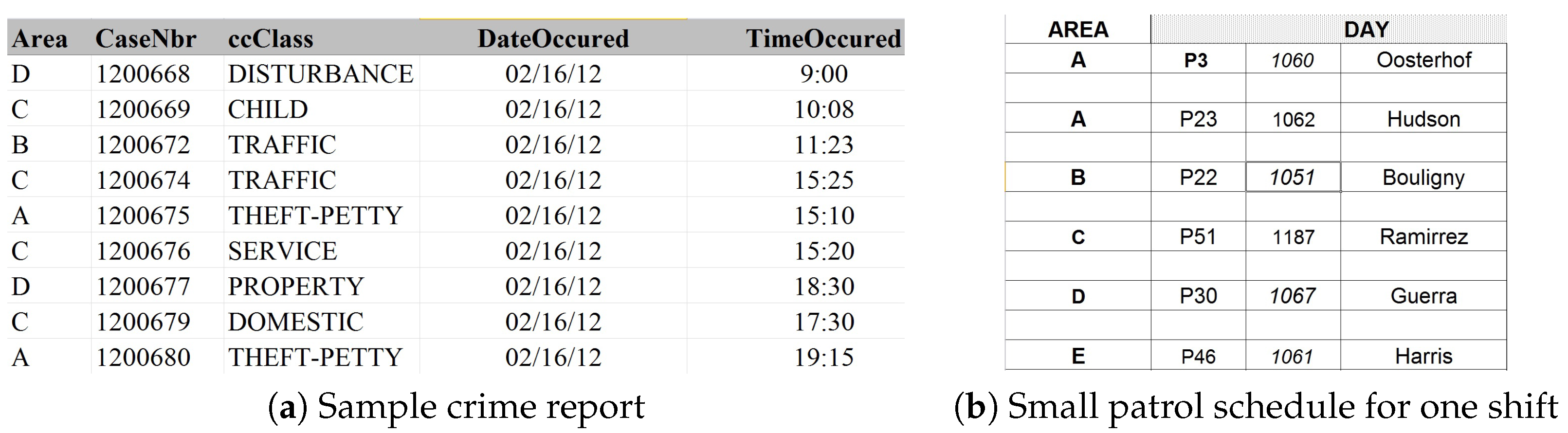
3.1. Domain Description

The motivating example for this study is the problem of controlling crime on a university campus. Our case study is about the American University, USC. USC has a Department of Public Safety (DPS) that conducts regular patrols, similar to police patrols in urban settings. As part of our collaboration with USC’s DPS, we have access to the crime report as well as patrol schedule on campus for three years (2011 to 2013). USC is a large enough university that we can claim that our methods are applicable to other campuses similar in size, for example malls.
USC’s campus map is divided into five patrol areas, which is shown in Figure 1. DPS patrols in three shifts per day. Crime data are exclusively local, i.e., no crime happens across two patrol areas or patrol shifts. At the beginning of each patrol shift, DPS assigns each available patrol officer to a patrol area, and the officer patrols this area in this shift. At the same time, the criminal is seeking for crime opportunities by deciding which target they want to visit. Discussions with DPS reveal that criminals act opportunistically, i.e., crime is not planned in detail, but occurs when an opportunity arises and there is insufficient presence of DPS officers.
There are two reports that DPS shared with us. The first is about criminal activity that includes the details of each reported crime during the last three years, including the type of crime and the location and time information about the crime. We show a snapshot of these data in Figure 2a. In this paper, we do not distinguish between the different types of crime, and hence, we consider only the number of crimes in each patrol area during each shift. Therefore, we summarize the three-year crime report into 365 × 3 × 3 = 3285 crime data points, one for each of the eight-hour patrol shift. Each crime data point contains five crime numbers, one for each patrol area.
The second dataset contains the DPS patrol allocation schedule. Every officer is allocated to patrolling within one patrol area. We show a snapshot of these data in Figure 2b. We assume that all patrol officers are homogeneous, i.e., each officer has the same effect on criminals’ behavior. As a result, when generating a summary of officer patrol allocation data, we record only the number of officers allocated to each patrol area in each shift.
Table 1 shows a sample of the summarized crime data, where the row corresponds to a shift, the columns correspond to a patrol area and the numbers in each cell are the number of crimes. Table 2 shows a sample of the summarized officer patrol allocation data, where rows correspond to shifts, columns correspond to patrol areas and the numbers within a cell represent the number of patrol officers present. For example, from Table 2, we know that in Shift 1, the number of officers in area A is two, while the number of officers in areas B, C, D and E is one; while from Table 1, we know that in Shift 1, there was one crime each in areas A and B and two crimes each in C, D and E. However, we do not know the number of criminals in any patrol area in any patrol shift. We call the patrol areas the targets and each patrol shift a time step.

3.2. Problem Statement

Given data such as the real-world data from USC, our goal is to build a general learning and planning framework that can be used to design optimal defender patrol allocations in any comparable urban crime setting. In the first cut, we model the learning problem as a Markov chain. Next, we use a DBN to model criminals’ behavior and also present a compact form of DBN that leads to improved prediction. The DBN approach yields better results than the Markov chain approach. Finally, we present methods to find the optimal defender plan for the learned model with the frequent update of the criminal model.

4. Learning Model

As stated earlier, we propose two approaches to learn the interaction between criminals and defenders: MCM and DBNM, which we explain in detail in the next two sub-sections. Both approaches are Markov process, but the first approach MCM learns the crime distribution using only observed data, while DBNM uses the number of criminals as an unobserved (hidden or latent) state. As a consequence, the learning algorithm for MCM uses simple maximum likelihood estimation, while DBNM uses the expectation maximization.

4.1. Markov Chain Models (MCM)

The models presented can be divided into three sub-categories: (1) crime as a function of crime history; (2) crime as a function of defender allocation; and (3) crime as a function of crime history and defender allocation jointly. One motivation for this classification is to figure out the correlation between previous-time crime and previous or current-time defenders in the targets and to find out if the presence of patrol officers affects the pattern of crime or not. We discuss these modeling approaches in the following sub-sections.

4.1.1. Crime Predicts Crime

In the first model shown in Figure 3a, we investigate the prediction of crime based on the crime distribution at the previous time step at the same target. This correlation is suggested based on the “crime predicts crime” ideas introduced in the criminology literature [17]. The desired correlation can be defined with the following mathematical function for all targets n: Y n , t + 1 = f ( Y n , t ) .
To define and formalize the correlation and a pattern for crime prediction from history, we define a transition matrix, A, that represents how crime occurrences change from one time step to the next one and apply maximum likelihood estimation to obtain it. In particular, A ( Y n , t , Y n , t - 1 ) = P ( Y n , t | Y n , t - 1 ) .
For this model, the probability for a sequence of events, i.e., Y n , which refers to number of crimes over a sequence of time steps, can be calculated as follows:
P ( Y n ; A ) = P ( Y n , t , . . . , Y n , 0 ; A ) = 1 t T P ( Y n , t | Y n , t - 1 ; A ) = 1 t T A ( Y n , t , Y n , t - 1 )
In the above equations, n indicates the target number, and A is the parameter to be estimated. The log likelihood for the above model for target i can be written as the following:
l ( A ) = log P ( Y n ; A ) = i = 1 | S Y | j = 1 | S Y | t = 1 T 1 { Y n , t = S i Y n , t - 1 = S j } log A i j
where S i and S j indicate different values that Y can take and S Y indicates the total possible number of values that Y can take; one is the indicator function. As previously mentioned, in our case, we made a binary assumption for variables, so they can take values of zero and one. The optimization problem for maximizing the log-likelihood is:
max A l ( A ) subject to i = 1 | S Y | A i , j = 1 for j = 1 . . . | S Y | , A i j 0 for i , j = 1 . . . | S Y |
The above optimization can be solved in closed form using the method of Lagrangian multipliers to obtain:
A i j ^ = t = 1 T 1 { Y t = S i Y t - 1 = S j } t = 1 T 1 { Y t - 1 = S j }
For each target, we find a similar transition matrix. For all other models in this section, the same procedure for deriving the transition matrix is used. The model shown in Figure 3b includes the number of crimes at all other targets. This approach can be described with the following mathematical function: Y n , t + 1 = f ( Y 1 : n , t ) .

4.1.2. Defender Allocation Predicts Crime

In the second approach, we study the prediction of the crime based on the defender allocation. Four cases are studied: in Figure 3c, Y n , t + 1 = f ( D n , t + 1 ) , which means the effect of the defender at the same target and time step is considered; in Figure 3d, Y n , t + 1 = f ( D n , t ) , which means the defender allocation at the previous step is considered; in Figure 3e, Y n , t + 1 = f ( D n , t , D n , t + 1 ) , which means the defender allocation in both the current and previous time step is considered; in Figure 3f, Y n , t + 1 = f ( D 1 : n , t , D n , t + 1 ) , meaning the defender allocation at all other targets from the previous time step and the defender allocation from the current time is considered. The same procedure as the previous subsection is used to find the transition matrix for the above models.

4.1.3. Crime and Defender Allocation Predicts Crime

In this sub-section, we study the effect of crime and defender distribution jointly and investigate whether this combination improves the prediction. In Figure 3g, Y n , t + 1 = f ( D n , t + 1 , Y n , t ) , which means that the distribution of the crime at the previous step and the defender allocation at the current step is considered; in Figure 3h, Y n , t + 1 = f ( D n , t , Y n , t ) ; this has a similar structure as the previous one, except that it considers the defender allocation at the previous time step; in Figure 3i, Y n , t + 1 = f ( D n , t , D n , t + 1 , Y n , t ) , that is the crime at that specific target is considered in addition to the defender allocation at the previous and current step.

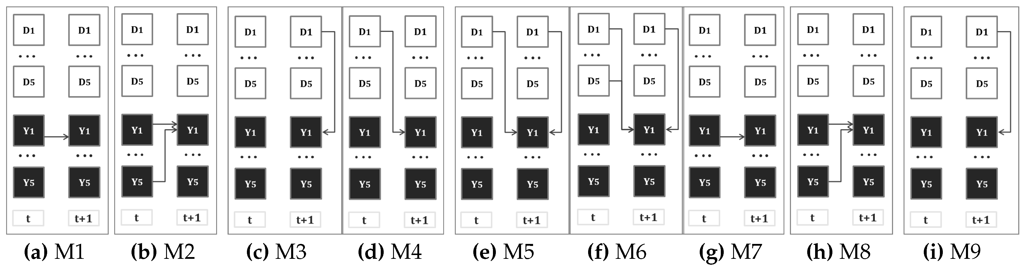
4.2. Dynamic Bayesian Network Models (DBNM)

The second approach is based on the Dynamic Bayesian Network (DBN) model. A DBN is proposed in order to learn the criminals’ behavior, i.e., how the criminals pick targets and how likely are they to commit a crime at that target. This behavior is in part affected by the defenders’ patrol allocation. In this section, we assume that criminals are homogeneous, i.e., all criminals behave in the same manner.
In every time step of the DBN, we capture the following actions: the defender assigns patrol officers to protect N patrol areas, and criminals react to the defenders’ allocation strategy by committing crimes opportunistically. Across time steps, the criminal can move from any target to any other, since a time step is long enough to allow such a move. From a game-theoretic perspective, the criminals’ payoff is influenced by the attractiveness of targets and the number of officers that are present. These payoffs drive the behavior of the criminals. However, rather than model the payoffs and potential bounded rationality of the criminals, we directly learn the criminal behavior as modeled in the DBN.
The DBN is shown in Figure 4: squares are observed states, where N white squares represent input states (number of defenders at each target) and N black squares represent output states (number of crime at each target), while N circles (number of criminals at each target) are hidden states. For ease of exposition, we use C to denote the largest value that any state can take. Next, we introduce the various parameters of this DBN.

4.2.1. DBN Parameters

First, we introduce parameters that measure the size of the problem:
  • N: Total number of targets in the graph.
  • T: Total time steps of the training data.
Next, we introduce random variables for the observed state (input defender distribution and output crime distribution in our case) and the hidden state. We use three random variables to represent the global state for defenders, criminals and crimes at all targets.
  • d t : Defender’s allocation strategy at step t: the number of defenders at each target in step t with C N possible values.
  • x t : Criminals’ distribution at step t with C N possible values.
  • y t : Crime distribution at step t with C N possible values.
Next, we introduce the unknown parameters that we wish to learn.
  • π: Initial criminal distribution: probability distribution of x 1 .
  • A (movement matrix): The matrix that decides how x t evolves over time. Formally, A ( d t , x t , x t + 1 ) = P ( x t + 1 | d t , x t ) . Given the C N values for each argument of A, representing A requires C N × C N × C N parameters.
  • B (crime matrix): The matrix that decides how criminals commit crime. Formally, B ( d t , x t , y t ) = P ( y t | d t , x t ) . Given the C N values for each argument of B, representing B requires C N × C N × C N parameters.
Next, we introduce variables that are used in the EM algorithm itself. These variables stand for specific probabilities as illustrated below. We use d i j ( y i j ) as shorthand for d i , , d j ( y i , , y j ):
  • Forward prob.: α ( k , t ) = P ( y 1 t , x t = k | d 1 t ) .
  • Backward prob.: β ( k , t ) = P ( y t + 1 T | x t = k , d t + 1 T ) .
  • Total prob.: γ: γ ( k , t ) = P ( x t = k | y 1 T , d 1 T ) .
  • Two-step prob.: ξ ( k , l , t ) = P ( x t = k , x t + 1 = l | y 1 T , d 1 T ) .
We can apply the EM algorithm to learn the unknown initial criminal distribution π, movement matrix A and output matrix B. However, EM applied to the basic DBN model above results in practical problems that we discuss in the next section.

4.2.2. Expectation Maximization

EM is a class of algorithms for finding maximum likelihood estimation for unknown parameters in DBN [18]. The EM algorithm has an initialization step, the Expectation (E) step and the Maximization (M) step. The initialization step chooses initial estimates for unknown parameters (π, A, B). The E step computes α, β, γ, ξ using these estimates. The M step updates the estimates of π, A, B using values of α, β, γ, ξ from the E step. By iteratively performing the E and M steps, the EM algorithm converges to a local maxima of the likelihood function for parameters in the DBN. The particular mathematical equations used in E and M depends on the underlying model [19].
Initialization Step: In our problem scenario, the EM algorithm is used to learn π, A and B from the given data for the observed states. The initial estimates of the variables should satisfy the following condition:
i π ^ ( i ) = 1 , x t + 1 A ^ ( d t , x t , x t + 1 ) = 1 , y t B ^ ( d t , x t , y t ) = 1
As EM only converges to local optima, we employ the standard method of running the algorithm with several randomly-chosen initial conditions in our experiments.
Expectation Step: In the expectation step, we calculate α, β, γ and ξ based on the current estimate of π, A and B, given by π ^ , A ^ and B ^ .
As is standard in inference in DBNs, α ( k , 1 ) is calculated in a recursive manner. Hence, we first calculate forward probability at Step 1, α ( k , 1 ) , which is shown in Equation (6). Next, we iteratively compute forward probability from Step 2 to T, which is shown in Equation (7). A similar technique works for backward probability: first, we calculate backward probability at Step T, β ( k , T ) , which is shown in Equation (8). Then, we recursively calculate backward probability from Step T - 1 to 1, which is in Equation (9).
α ( k , 1 ) = P ( y 1 , x 1 = k | d 1 ) = B ^ ( d 1 , k , Y 1 ) · π ^ ( k ) α ( k , t ) = P ( y 1 , y 2 , . . . , y t , x t = k | d 1 , d 2 , . . . , d t )
= x t - 1 α ( x t - 1 , t - 1 ) A ^ ( d t - 1 , x t - 1 , x t ) B ^ ( d t , k , y t )
β ( k , T ) = 1 β ( k , t ) = P ( y t + 1 , y t + 2 , . . . , y T | x t = k , d t , d t + 1 , . . . , d T ) =
x t + 1 β ( x t + 1 , t + 1 ) B ^ ( d t + 1 , x t + 1 , y t + 1 ) A ^ ( d t , k , x t + 1 )
Given the forward probability and the backward probability at each step, the total probability γ is computed as shown in Equation (10), and the two-step probability ξ is computed as shown in Equation (11).
γ ( k , t ) = P ( x t = k | y , d ) = α ( k , t ) · β ( k , t ) k α ( k , t ) · β ( k , t ) ξ ( k , l , t ) = P ( x t = k , x t + 1 = l | y , d )
= α ( k , t ) · A ( d t , k , l ) · β ( l , t + 1 ) · B ( d t + 1 , l , y t + 1 ) k α ( k , t ) · β ( k , t )
Maximization Step: In the maximization step, the estimate of π, A and B is updated using the probabilities we derive in the expectation step, as follows:
π ^ ( k ) = γ ( k , 1 )
A ^ ( d , k , l ) = t 1 d t = d ξ ( k , l , t ) t l 1 d t = d ξ ( k , l , t )
B ^ ( d , x , y ) = t 1 y t = y , d t = d γ ( x , t ) t 1 d t = d γ ( x , t )
where 1 d t = d is an indicator function: 1 d t = d = 1 when d t = d and zero otherwise. 1 y t = y , d t = d is also defined similarly. As a result, the new estimate of A ( d , k , l ) is the ratio of the expected number of transitions from k to l given defender vector d to the expected total number of transitions away from k given defender vector d. The updated estimate of B ( d , x , y ) is the ratio of the expected number of times the output of crimes equals to y, while the defender is d, the criminal is x to the total number of situations where the defender is d and the criminal is x. To find a local optimal solution, the E and M steps are repeated, until π ^ , A ^ , B ^ do not change significantly any more.
In the EM algorithm, the size of movement matrix A is C N × C N × C N , and the size of crime matrix B is also C N × C N × C N . The number of unknown variables is O ( C 3 N ) . The exponentially many parameters make the model complex and, hence, results in over-fitting given limited data. In addition, the time complexity, as well as the space complexity of EM depend on the number of parameters; hence, the problem scales exponentially with N. In practice, we can reduce C by categorizing the number of defenders, criminals and crimes. For example, we can partition the number of defenders, criminals and crimes into two categories each: the number of officers at each station is one (meaning ≤1) or two (meaning ≥2); the number of criminals/crimes is zero (no criminal/crime) or one (≥1 criminal/crime). However, the number of unknown parameters is still exponential in N. As a concrete example, at USC, N = 5 , and the number of unknown parameters are more than 32,768, even when we set C = 2 . As we have daily data for three years, which is 365 × 3 × 3 = 3285 data points, the number of parameters is much more than the number of data points. Therefore, we aim to reduce the number of parameters to avoid over-fitting and accelerate the computing process.

4.2.3. EM on the Compact Model

In this part, we modify the basic DBN model to reduce the number of parameters. In the resultant compact model, the EM learning process runs faster and avoids over-fitting to the given data. The improvement may be attributed to the well-established learning principle of Occam’s razor [20] and our experimental results support our claims.
Compact model: We use three modifications to make our model compact. (1) We infer from the available crime data that crimes are local, i.e., crime at a particular target depends only on the criminals present at that target. Using this inference, we constructed a factored crime matrix B that eliminates parameters that capture non-local crimes. (2) Next, we rely on intuition from the Boyen–Koller [6] (BK) algorithm to decompose the joint distribution of criminals over all targets into a product of independent distributions for each target. (3) Finally, our consultations with the DPS at USC and prior literature on criminology [1] led us to conclude that opportunistic criminals by and large work independently. Using this independence of behavior of each criminal (which is made precise in Lemma 1), we reduce the size of the movement matrix. After these steps, the number of parameters is only O ( N · C 3 ) .
Before describing these modifications in detail, we introduce some notations that aid in describing the different quantities at each target: Y t = [ Y 1 , t , Y 2 , t , . . . , Y N , t ] is an N by one random vector indicating the number of crimes Y i , t at each target i at step t. D t is an N by one random vector indicating the number of defenders D i , t at each target i at step t. X t is an N by oen random vector indicating the number of criminals X i , t at each target i at step t.
Factored crime matrix: The number of crimes at one target at one step is only dependent on the criminals and officers present at that target at that step. Therefore, we factor the crime matrix B to a matrix that has an additional dimension with N possible values, to represent how the criminals and officers at one target decide the crime at that target. Therefore, instead of the original crime matrix B of size C N × C N × C N , we have a factored crime matrix of size N × C × C × C . The first dimension of the factored crime matrix represents the target; the second dimension represents the number of defenders at this target; the third dimension represents the number of criminals; and the fourth dimension represents the number of crimes. We still refer to this factored crime matrix as B, where B ( i , D i , t , X i , t , Y i , t ) = P ( Y i , t | D i , t , X i , t )
Marginalized hidden state: The BK algorithm presents an approximation method by keeping the marginals of the distribution over hidden states, instead of the full joint distribution. Following the BK intuition, we marginalize the hidden state, i.e., instead of considering the full joint probability of criminals at all targets (with C N possible values), we consider a factored joint probability that is a product of the marginal probability of the number of criminals at each target.
In the unmodified DBN, the distribution over all of the states at step t, P ( x t ) is a C N by one vector. Additionally, the size of movement matrix A, which is the transition matrix from all of the input and hidden state combinations at the current step to the state at next step, is C N × C N × C N . After marginalization, the marginals for each target i in the hidden state are P ( X i = k , t ) , which is a vector of size C. After we marginalize the hidden states, we only need to keep N marginals at each step, i.e., consider only N parameters. At each step, we can recover the distribution of the full state by multiplying the marginals at this step. Then, we get the marginals at the next step by evolving the recovered joint distribution of the state at the current step. Therefore, A can be expressed as a C N × C N × N × C matrix, where A ( d t , x t , i , X i , t + 1 ) = P ( X i , t + 1 | d t , x t ) .
Pairwise movement matrix A m : Even with the marginalized hidden state, we still need to recover the distribution of the full state in order to propagate to next step. Therefore, the movement matrix size is still exponential with C N × C N × N × C . In order to further reduce the number of unknown parameters and accelerate the computing process, we use the properties of opportunistic criminals. Based on the crime reports and our discussion with DPS at USC, unlike organized terrorist attacks, the crimes on campus are committed by individual opportunistic criminals who only observe the number of defenders at the target they are currently at and do not communicate with each other. Therefore, at the current step, the criminals at each target independently decide the next target to go to, based on their target-specific observation of the number of defenders.
Based on the above observation, we can decompose the probability P ( X i , t + 1 = 0 | D t , X t ) into a product of probabilities per target m. Denote by X t + 1 m i the random variable that counts the number of criminals moving from target m to target i in the transition from time t to t + 1 . Lemma 1 proves that we can represent P ( X i , t + 1 = 0 | D t , X t ) as a product of probabilities P ( X t + 1 m i = 0 ) for each m. P ( X t + 1 m i = 0 ) is a function of D m , t , X m , t .
Lemma 1. 
(Independence of behavior) For a N target learning problem, given the number of defenders at each location D t = [ D 1 , t , . . . , D N , t ] and the number of criminals X t = [ X 1 , t , . . . , X N , t ] , the probability P ( X i , t + 1 = 0 | D t , X t ) of the number of criminal being zero at location i at step t + 1 is given by j = 1 N P ( X t + 1 j i = 0 ) .
Proof 1. 
Note that we must have X t + 1 m i 0 . We have the total number of criminals at target i at time step t + 1 as X i , t + 1 = m X t + 1 m i , i.e, the number of criminals at target i at step t + 1 is the sum of criminals that move from each target to target i. Clearly X i , t + 1 = 0 iff X i , t + 1 D m , t , X m , t = 0 . Therefore, we have P ( X i , t + 1 = 0 | D t , X t ) = P ( X t + 1 1 i = 0 , , X t + 1 N i = 0 ) . Since the criminals’ decisions at each target are independent, we have P ( X t + 1 1 i = 0 , . . . , X t + 1 N i = 0 ) = m = 1 N P ( X t + 1 m i = 0 ) . ☐
When C = 2 and X i , t { 1 , 2 } , we can construct the whole movement matrix A using P ( X t + 1 m i = 0 ) (pairwise transition probabilities) by utilizing the fact that P ( X i , t + 1 = 1 | D t , X t ) = 1 - P ( X i , t + 1 = 0 | D t , X t ) . Therefore, instead of keeping A, we keep a transition matrix A m where A m ( i , D i , t , X i , t , j , X j , t + 1 ) = P ( X t + 1 i j ) . The number of parameters in A m is N × 2 × 2 × N = 4 N 2 . We do not consider the range of X j , t + 1 , because we only need one parameter to store the two cases of X j , t + 1 = 1 and X j , t + 1 = 0 since A m ( i , D i , t , X i , t , j , X j , t + 1 = 1 ) = 1 - A m ( i , D i , t , X i , t , j , X j , t + 1 = 0 ) . When C > 2 , the number of variables in A m are C 2 ( C - 1 ) N 2 ; we can extend Lemma 1 to any number of criminals at the next step using the concept of permutations; e.g., if there is one criminal at the next step, this means that there is only one station m where X t + 1 m i = 1 , and for all other stations, n m , X t + 1 n i = 0 . One simple example is when X i , t { 0 , 1 , 2 } ; we can apply Lemma 1 to derive:
P ( X i , t + 1 = 0 | D t , X t ) = j = 1 N P ( X i , t + 1 = 0 | D j , t , X j , t ) P ( X i , t + 1 = 1 | D t , X t ) = j = 1 N [ P ( X i , t + 1 = 1 | D j , t , X j , t ) k = 1 , k j N P ( X i , t + 1 = 0 | D k , t , X k , t ) ] P ( X i , t + 1 = 2 | D t , X t ) = 1 - P ( X i , t + 1 = 0 | D t , X t ) - P ( X i , t + 1 = 1 | D t , X t )

4.2.4. EMC 2 Procedure

The EM on CompaCtmodel (EMC 2 ) procedure applies the EM algorithm to the compact DBN model. To learn the initial distribution π k , i = P ( X i , 1 = k ) , matrix A m and matrix B, we first generate initial estimates of these parameters that satisfy the condition k π ^ ( k , i ) = 1 , X j , t + 1 A ^ m ( i , D i , t , X i , t , j , X j , t + 1 ) = 1 and Y i , t B ^ ( i , D i , t , X i , t , Y i , t ) = 1 .
Next, we define the intermediate variables used in the EM algorithm. These differ from the earlier application of EM because of our changed model. We use the shorthand Y i j to denote Y i , . . . , Y j and D i j to denote D i , . . . , D j :
  • Forward prob.: α ( i , k , t ) = P ( Y 1 t , X i , t = k | D 1 t ) .
  • Backward prob.: β ( i , k , t ) = P ( Y t + 1 T | X i , t = k , D t T ) .
  • Total prob.: γ ( i , k , t ) = P ( Y , X i , t = k | D 1 T ) .
  • Two-step prob.: ξ ( i , k , j , l , t ) = . P ( X i , t = k , X j , t + 1 = l | Y 1 T , D 1 T ) .
Next, the E and M steps are used with random restarts to learn the values of π, A m and B. While the equations used in the E and M steps can be derived following standard EM techniques, we illustrate a novel application of the distributive law for multiplication in the E step that enables us to go from exponential time complexity to polynomial (in N) time complexity. Without going into the details of the algebra in the E step, we just focus on the part of the E step that requires computing P ( Y 1 t - 1 , X i , t = 0 | D 1 t ) .
The following can be written from total law of probability:
P ( Y 1 t - 1 , X i , t = 0 | D 1 t ) = X t - 1 P ( Y 1 t - 1 , X i , t = 0 , X t - 1 | D 1 t ) = X t - 1 P ( Y 1 t - 1 | D 1 t , X i , t = 0 , X t - 1 ) P ( X i , t = 0 | D 1 t , X t - 1 ) P ( X t - 1 | D 1 t )
The above can be simplified using the Markovian assumptions of the DBN to the following:
X t - 1 P ( Y 1 t - 1 | D 1 t , X t - 1 ) P ( X i , t = 0 | D t - 1 , X t - 1 ) P ( X t - 1 | D 1 t )
The first and third term can be combined (Bayes theorem) to obtain:
X t - 1 P ( Y 1 t - 1 , X t - 1 | D 1 t ) P ( X i , t = 0 | D t - 1 , X t - 1 )
Using the Boyen–Koller assumption in our compact model, we get:
P ( Y 1 t - 1 , X t - 1 | D 1 t ) = j P ( Y 1 t - 1 , X j , t - 1 | D 1 t )
Furthermore, using Lemma 1, we get:
P ( X i , t = 0 | D t - 1 , X t - 1 ) = j P ( X t j i = 0 )
Thus, using these, we can claim that P ( Y 1 t - 1 , X i , t = 0 | D t ) is:
X t - 1 j P ( Y 1 t - 1 , X j , t - 1 | D 1 t ) P ( X t j i = 0 )
Since the range of X t - 1 is C N , naively computing the above involves summing C N terms, thus implying a time complexity of O ( C N ) . The main observation that enables polynomial time complexity is that we can apply the principles of the generalized distributive law [21] to reduce the computation above. As an example, the three summations and four multiplication in a b + a c + b c + b d can be reduced to two summations and one multiplication by expressing it as ( a + b ) ( c + d ) . Using the distributive law, we reduce the computation for P ( Y 1 t - 1 , X i , t = 0 | D 1 t ) by switching the sum and product:
j X j , t - 1 P ( Y 1 t - 1 , X j , t - 1 | D 1 t ) P ( X t j i = 0 )
The complexity of computing the above is O ( N C ) . Applying this idea, we can calculate α, β, γ and ξ from the estimated value of π ^ , A m ^ and B ^ in the expectation step in time polynomial in N.
For the maximization step, we update the estimate of π, A m and B using the probabilities we derive in the expectation step. The procedure is the same as Equations (7) to (9). In the following part, we provide the detail of EMC 2 procedure.
Initialization step: Set random initial conditions for criminal distribution π, transition matrix A and output matrix B. See Appendix A for an example of one such initialization.
Expectation step: The main idea of the expectation step is to calculate the forward probability α and backward probability β based on the estimation of π, A and B. This is explained below.
Step 1: Iteratively calculating forward probability
First, we calculate the forward probability at Step 1 ( α ( i , k , 1 ) ) as:
α ( i , k , 1 ) = P ( Y 1 , X i , 1 = k | D 1 ) = P ( Y i , 1 , X i , 1 = k | D i , 1 ) = P ( Y i , 1 | X i , 1 = k , D i , 1 ) · P ( X i , 1 = k | D i , 1 ) = B ( i , D i , 1 , k , Y i , 1 ) · π ( k , i )
Then, we iteratively calculate the forward probability from Step 2 to T denoted as α ( i , k , t ) . We then apply dynamic programming to go one step forward. In order to do this, we use P ( Y 1 , Y 2 , . . . , Y t - 1 , X i , t | D 1 , D 2 , . . . , D t - 1 ) as an intermediate variable. Details are in the Appendix A.
Step 2: Iteratively calculating backward probability
First, we calculate backward probability at step T( β ( i , k , T ) ) as follows:
β ( i , k , T ) = 1
Then, we iteratively calculate the backward probability at each time step t ( β ( i , k , t ) ) from Step T-1 to 1. Detailed calculations are provided in Appendix A.
Step 3: Calculating total probability γ
The total probability γ ( i , k , t ) is then calculated. Detailed calculations are shown in the Appendix.
Step 4: Calculating two-step probability ξ
Finally, we calculate the two-step probability ξ. We show the detailed calculations in the Appendix.
Maximization step: The main idea of the maximization step is to update the new estimation of π, transition matrix A and output matrix B based on new-calculated forward/backward probability α and β.
Step 1: Update the initial state distribution:
π ( k , i ) = γ ( i , k , 1 )
by definition, π is γ at Step 1, which is the expected frequency of value k at Time 1.
Step 2: Update output matrix B:
B ( i , d i , t , x i , t , y i , t ) = t 1 Y i , t = y i , t , D i , t = d i , t γ ( i , x i , t , t ) t 1 D i , t = d i , t γ ( i , x i , t , t )
1 Y i , t = y i , t , D i , t = d i , t = 1 , Y i , t = y i , t , D i , t = d i , t 0 , o t h e r w i s e
1 D i , t = d i , t = 1 , D i , t = d i , t 0 , o t h e r w i s e
where 1 Y i , t = y i , t , D i , t = d i , t is an indicator function and B ( i , d , x , y ) is the expected number of times the output of crimes has been equal to y while the defender is d and the criminal is k over the expected total number of times at target i.
Step 3: Update transition matrix A:
A ( m , d m , t , x m , t , i , x i , t + 1 ) = t 1 D t = d t ξ ( m , d m , t , x m , t , i , x i , t + 1 ) ) t x i , t + 1 1 D t = d t ξ ( m , d m , t , x m , t , i , x i , t + 1 ) )
which is the expected number of transitions from x t to k given defender vector d t compared to the expected total number of transitions away from x t given defender vector d t .
Repeat: Repeat the expectation step and the maximization step, which is π , A , B α , β , γ , ξ π , A , B , until π , A , B do not change anymore. This means we reach the local optimal solution.
Computational complexity analysis: EM on basic model: In the basic model, the time complexity of the E step is O ( C 2 N T ) . The time complexity for the M step is also O ( C 2 N T ) . Thus, the computational complexity for the EM algorithm is O ( C 2 N T ) ; EMC 2 procedure: In the EMC 2 procedure, the time complexity for the E step is O ( N C + 1 T ) . α and β in Equations 11 and 13 are O ( N C ) . Since we have to compute α ( i , k , t ) and β ( i , k , t ) for all i N , k = 1 , 2 and t T , the computational complexity for forward and backward probability is O ( N C + 1 T ) . For Equation (14), the complexity is O ( 1 ) , and the complexity for γ is O ( N T ) . For Equation (15), the complexity is O ( N ) , and the complexity for ξ is O ( N C + 1 T ) . The total complexity for the E step is O ( N C + 1 T + N T + N C + 1 T ) = O ( N C + 1 T ) . The time complexity for the M step is O ( ( C · N ) 2 T ) . Thus, the computational complexity for the EM algorithm is O ( N C + 1 T + ( C · N ) 2 T ) . Therefore, the EMC 2 procedure runs much faster than the EM in the basic model when C is small.

5. Dynamic Planning

The next step after learning the criminals’ behavior is to design effective officer allocation strategies against such criminals. In this section, we first introduce a simple online planning mechanism, in which we iteratively update the criminals’ behavior model and plan allocation strategies. Next, we present a slower optimal planning algorithm and a faster, but sub-optimal greedy algorithm.
Online planning mechanism: We first state our template for iterative learning and planning before describing the planning algorithms. The criminal behavior may change when the criminal observes and figures out that the defender strategy has changed. Thus, the optimal strategy planned using the learned parameters is no longer optimal after some time of deployment of this strategy, as the parameters themselves change in response to the deployed strategy.
To address the problem above, we propose an online planning mechanism. In this mechanism, we update the criminal’s model based on real-time crime/patrol data and dynamically plan our allocation strategy. The first step is to use the initial training set to learn an initial model. Next, we use a planning algorithm to generate a strategy for the next T u steps. After executing this strategy, we can collect more crime data and use them to update the model with the original training data. By iteratively doing this, we generate strategies for the whole horizon of T steps. Algorithm 1 presents the details of this mechanism.
Algorithm 1 Online planning ( T r a i n _ d a t a , T u , T ).
1: A , B , π L e a r n ( T r a i n _ d a t a )
2: t = 0
3:while t < T do
4:     [ D 1 , . . . , D T u ] P l a n ( A , B , π )
5:     [ Y 1 , . . . , Y T u ] E x e c u t e { D 1 , . . . , D T u }
6:     T r a i n _ d a t a T r a i n _ d a t a { D 1 , Y 1 , . . . , D T u , Y T u }
7:     A , B , π U p d a t e ( T r a i n _ d a t a , A , B , π )
8:     t = t + T u
9:end while
Compared to simply applying the planning algorithm for T steps, our online planning mechanism updates the criminals’ behavior model periodically based on their response to the currently-deployed strategy. In this online planning mechanism, three parts are needed: learning algorithm, updating algorithm and planning algorithm. For the learning and updating algorithms, we apply the EMC 2 learning algorithm from Section 5. In addition, we also need a planning algorithm, which we discuss next.

5.1. Planning Algorithms

5.1.1. The Planning Problem

In the planning problem, the criminals’ behavior is known or, more specifically, we already know the criminals’ initial distribution π, movement matrix A and crime matrix B in the DBN model. Given a pure defender patrol allocation strategy for T u steps, we can plug those values for the input state into the DBN and get the expected number of crimes in T u steps. The goal of planning is to find the defenders’ pure strategy that optimizes the defenders’ utility, which in our case is to minimize the total expected number of crimes (in our framing, any randomized strategy, which is the combination of pure strategies, results in a greater number of crimes than the optimal pure strategy). Thus, planning against opportunistic criminals is a search problem in the defender’s pure strategy space. First, we present the practical impossibility of a brute force search.

5.1.2. Brute Force Search

A naive way to solve this problem is to try all possible allocation strategies and to pick the one that leads to the least crimes in T u steps. However, since at each step, the number of possible allocation strategies is C N and there are T u steps in total, the strategy space is C N T u . For example, for our specific problem of patrolling in USC with five targets, two categories and the goal of planning for T u = 300 steps, we need to search 2 1500 10 451 different strategies, which is impractical to solve.

5.1.3. Dynamic Opportunistic Game Search (DOGS)

First, we list some notation that will be used in the next two planning algorithms.
  • D t j indicates the j-th strategy for the defender from the C N different defender strategies at time step t.
  • P j , t is the total number of crimes corresponding to the optimal defender strategy for the first t time steps that has j as its final defender strategy.
  • X j , t is the criminals’ location distribution corresponding to the optimal defender strategy for the first t time steps that has j as its final defender strategy.
  • f Y ( X t , D , B ) is the expected number of crimes at all targets at t given the criminal location distribution X t and defender’s allocation strategy D at step t and output matrix B.
  • f X ( A , X t , D t ) is the criminal location distribution at step t + 1 given the criminal location distribution X t and defender’s allocation strategy D t at t and transition matrix A.
Algorithm 2 DOGS ( A , B , π ).
1:for each officer allocation D 1 i do
2:     Pa [ i , 1 ] 0 ; P i , 1 f Y ( A , π , D 1 i ) ; X i , 1 π
3:end for
4:for t 2 , 3 , . . . , T u do
5:    for each officer allocation D t j do
6:         F ( i ) = f Y ( f X ( A , X i , t - 1 , D t - 1 i ) , D t j , B ) + P i , t - 1
7:         Pa [ D t j , t ] argmin i [ F ( i ) ] ; P j , t min i [ F ( i ) ]
8:         X j , t f X ( A , X Pa [ D t j , t ] , t - 1 , D t - 1 Pa [ D t j , t ] )
9:    end for
10:end for
11: i n d e x [ T ] argmin i P i , T ; D ^ [ T ] D T i n d e x [ T ]
12:for t T - 1 , . . . , 1 do
13:     i n d e x [ t ] Pa [ D t i n d e x [ t + 1 ] , t + 1 ]
14:     D ^ [ t ] D t i n d e x [ t ]
15:end for
16:return D ^
DOGS is a dynamic programming algorithm; hence, in order to find the optimal strategy for t steps, we first find the optimal strategy for the sub-problem with t - 1 steps and use it to build the optimal strategy for t steps. Given the values of π, A and B from our learning step, the optimal defender allocation strategy D 1 , . . . , D T u is given by the recurrence relations:
P j , 1 = f Y ( π , D 1 j , B ) P j , t = min i [ f Y ( f X ( A , X i , t - 1 , D t - 1 i ) , D t j , B ) + P i , t - 1 ]
Retrieving the optimal allocation strategy requires remembering the allocation D t - 1 i that minimizes the second equation, which is done by storing that information in the function Pa , as follows:
Pa [ j , t ] = arg min i [ f Y ( f X ( A , X i , t - 1 , D t - 1 i ) , D t j , B ) + P i , t - 1 ]
As P j , T u is the total number of crimes for the optimal defender strategies for T u time steps that has j as the final strategy, the optimum strategy for time step T u is given by D T u = arg min j P j , T u . Then, recursively, given optimal D t , we find the optimal strategy in the previous time step using function Pa : D t - 1 = Pa [ D t , t ] . The complexity of the DOGS algorithm (Algorithm 2) is O ( C 2 N T u ) .

5.1.4. Greedy Search

The dynamic programming-based algorithm can generate the optimal strategy, but takes time O ( C 2 N T u ) . We present a greedy algorithm that runs in O ( C N T u ) time, but the solution may be sub-optimal. In the greedy search, we split the strategy space into T u slices. Each slice represents the strategy at each step. Then, instead of searching the optimal strategy for T u steps, we only look one step ahead to search for the strategy that optimizes the defender’s utility at the current step (Algorithm 3). It finds the optimal patrol allocation D t at the current step by minimizing the expected number of crimes at all targets at step t. For the next step, we compute the criminal’s distribution X t + 1 and greedily search again. We keep iterating this process until we reach the T u step. The complexity of greedy search is O ( C N T u ) .
Algorithm 3 Greedy ( A , B , π = X 1 ).
1:for t 1 , , T u do
2:     D t argmin D f Y ( X t , D , B ) ; X t + 1 f X ( A , X t , D t )
3:end for
4:return D = [ D 1 , . . . , D T u ]

6. Experimental Results

6.1. Experimental Setup

All of our experiments were performed on a machine with 2.4 GHz and 16 GB RAM. MATLAB was our choice of programming language. There are two threads of experiments, one on learning and the other on learning and planning. To avoid leaking confidential information of the USC Department of Public Safety, all of the crime numbers shown in the results are normalized.

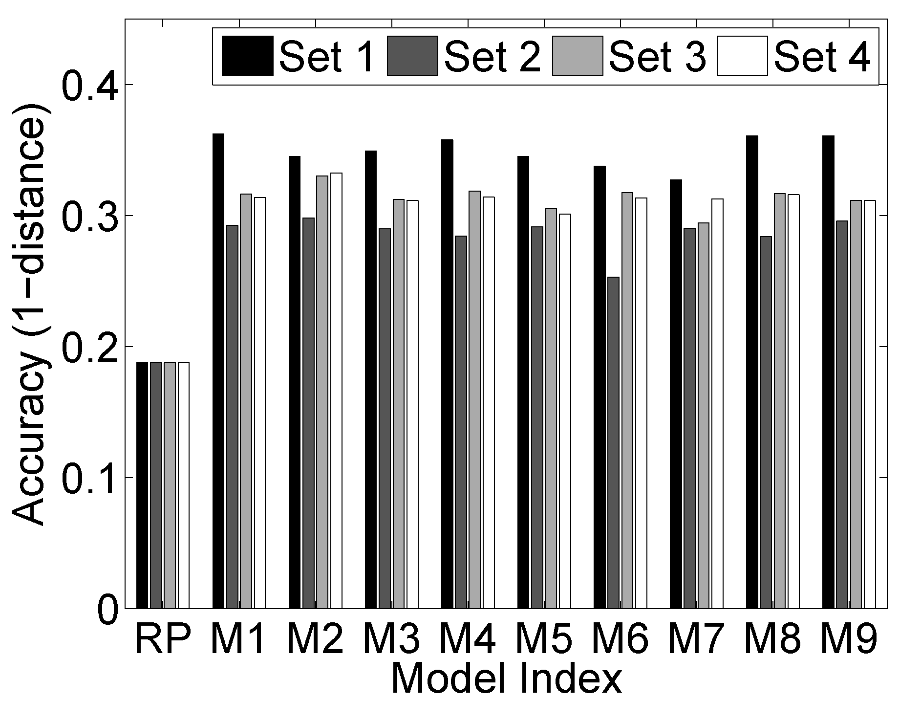
6.2. Learning (Setting)

Our first experiment is on evaluating the performance of the EMC 2 algorithm in learning criminals’ behavior. We use the case study of USC in our experiments. We obtained three years of crime reports and the corresponding patrol schedule followed at USC. Since the EMC 2 algorithm and the EM algorithm only reach the locally optimal solution, we run the algorithms for 30 different randomly-chosen start points and choose the best solution from among these runs. These start points, i.e., the values of A, B and π, are generated by sampling values from a uniform random distribution over [ 0 , 1 ] for all of the elements and then normalizing the probabilities so that they satisfy the initial conditions. C is set to two by default, while the effect of varying C is compared in Figure 5e.
The results shown in Figure 5a compare the estimated numbers of crimes using different learning algorithms with the real number of crimes in one month. We divide the three-year data into four equal parts of nine months each. For each part, we train on the first eight months data and test on the ninth month’s data. That is why the estimated number of crimes for one month as the output by different learning algorithms is compared to the real number of crimes in that month. The x-axis in this figure indicates the index of the part of the data that we evaluate. The y-axis is the total number of crimes in the ninth month. The closer this number is to the real number of crimes, the better the prediction is. Three different algorithms are compared: (1) the Markov Chain (MC) algorithm, in which the best performance among all eight models is shown; (2) the exact EM algorithm; and (3) the EMC 2 algorithm. As can be seen, the prediction of EMC 2 is much closer compared to those of the EM and MC algorithms in all of the training groups. This indicates that the crime distribution is related to the criminals’ location, and including the number of criminals at each target as a hidden state helps to improve the performance. In addition, the EMC 2 algorithm achieves better performance than EM by reducing the number of unknown variables to avoid over-fitting.
For Figure 5b, we measure the learning performance for each individual target using a metric that we call accuracy. To define this metric, let n i t be the actual number of crimes at target i for time step t; let n i t be the predicted number of crimes at target i at time step t. Then, accuracy at step t is the probability of the event i = 1 N | n i t - n i t | 1 . In other words, it is the probability that we make less than one mistake in predicting crimes for all N targets. The reported accuracy is the average accuracy over all t. In Figure 5b, the y-axis represents the accuracy. The higher accuracy is, the more accurate our prediction is. We compare four different algorithms: the MC, EM and EMC 2 algorithms and the uniform random algorithm, which sets equal probability for all possible numbers of crimes at each target. As expected, EMC 2 outperforms all other algorithms in all training groups. In addition, even though the accuracy of the algorithms varies in different training groups, which we attribute to the noisy nature of the data in the field, the largest difference is within 15 % . This indicates that accuracy of the algorithms is data-independent.
We present additional results under this setting in Figure 5c,d. We compare the four approaches for varying the size of training data; thus, the x-axis in both figures shows the number of training data (in days of data) used in learning. Our test data are all of the data points from a 30-day period, and the training data are the data points just before (in order of time) the test data points. For Figure 5c, the EMC 2 algorithm again outperforms all other algorithms for any number of training data in accuracy. In addition, the more data we have for training, the better accuracy we achieve. In Figure 5d, the y-axis shows the runtime in seconds on a log scale. The more data we have, the longer it takes for each training method. The random algorithm is pre-generated and takes almost no time; hence, those data are not shown in the figure; the runtime for MC is negligible because the number of states is small ( O ( 4 N ) ), and we traverse all of the data points only once; the runtime for the EMC 2 algorithm is significantly better than that for the EM algorithm, as is expected by our complexity analysis in Section 5.
In Figure 5e, we compare the four approaches by varying C. The x-axis shows the value of C. We use 1100 data points for training, while 30 data points, which are just after the training data points, are used for testing. The accuracy decreases as C increases. This is because when C increases, there are more possible values of the number of crimes. Thus, the possibility of predicting an accurate number decreases. However, when C increases from three to four, the decrease in accuracy is small in EMC 2 due to the fact that data with a value of four rarely appear in both the crime and patrol dataset. This indicates that a small C is a good approximation. In addition, the EMC 2 algorithm again outperforms all other algorithms for any C.
In Figure 6, all of the Markov chain models are compared. The x-axis is the model index. RP represents the uniform Random Predicting. M 1 through M 9 are the nine Markov chain models in Figure 3. The y-axis represents the accuracy. We use four sets of data that are the same as Figure 5b to test the performance. All of the Markov chain models give similar to accuracy, which outperforms RP significantly. However, as shown in Figure 5b, all of these models are outperformed by the EM and EMC 2 algorithms.

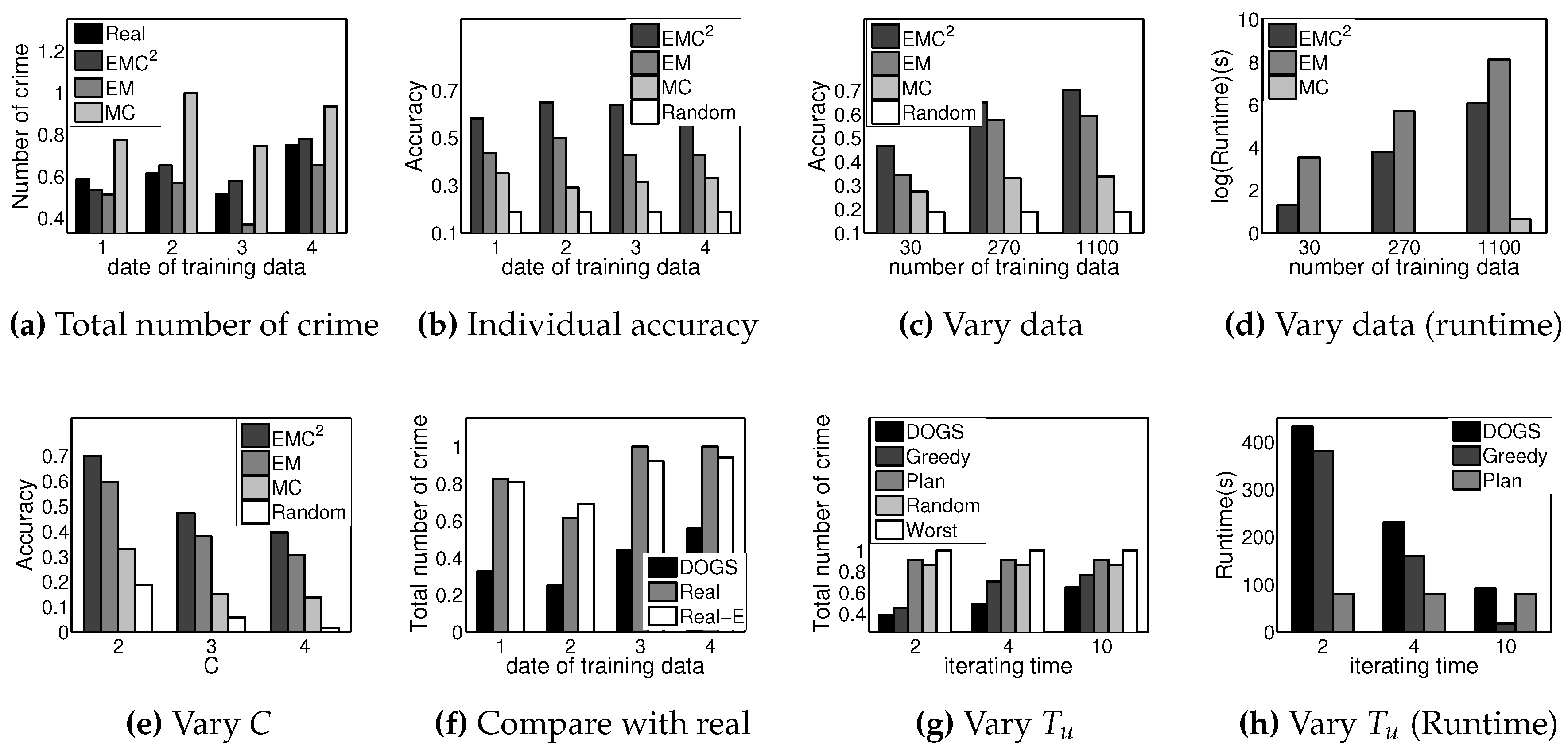
6.3. Learning and Planning (Real-World Data)

Figure 5f compares DOGS to the actual deployed allocation strategy generated by DPS experts at USC. Similar to the settings in Figure 5a, we divide the three-year data into four equal parts of nine months. For each part, we train on the first eight months’s data using the EMC 2 algorithm and test different allocation strategies on the first 10 days of the ninth month’s data. When testing the strategy, we assume the criminals’ behavior remains unchanged during these 10 days. Three different scenarios are compared: (1) the real number of crimes, shown as real in Figure 5f; (2) the expected number of crimes with the DPS strategy and learned criminal behavior, shown as real-E; and (3) the expected numbers of crime with DOGS allocation and learned criminal behavior, shown as DOGS. As shown in Figure 5f, the expected number of crimes with the DPS strategy is close to the real number of crimes, which indicates that EMC 2 captures the main features of the criminal behavior and provides a close estimate of the number of crimes. In addition, the DOGS algorithm outperforms the strategy generated by domain experts significantly. This demonstrates the effectiveness of the DOGS algorithm as compared to the current patrol strategy. By using the allocation strategy generated by DOGS, the total crime number reduces by ∼50% as compared to the currently-deployed strategy.

6.4. Learning and Planning (Simulated Data)

Next, we evaluate the performance of our online planning mechanism. We use simulations for this evaluation. In the simulation, the criminal model is simulated using the model from an earlier work on opportunistic criminals [2], in which the authors explicitly model an opportunistic criminal’s behavior. However, the defender does not know the type of criminals in our experiments. Instead, the defender starts by executing a random patrol schedule for 300 steps and collects the corresponding crime report, which they use to learn an initial criminal behavior model. The criminal responds to the defenders’ patrol schedule as predicted by the behavior model in [2]. Since the criminal behavior in [2] is probabilistic, we run the experiment 30 times, and each data point we report in this part is an average over these 30 instances. We fix the number of patrol officers to 2 N - 2 , where N is the number of targets. This number is consistent with our real dataset numbers (eight officers for five targets), where there were enough officers to allocate one officer to each target, but not enough to allocate two officers to each target. We use the EMC 2 algorithm as the learning algorithm.

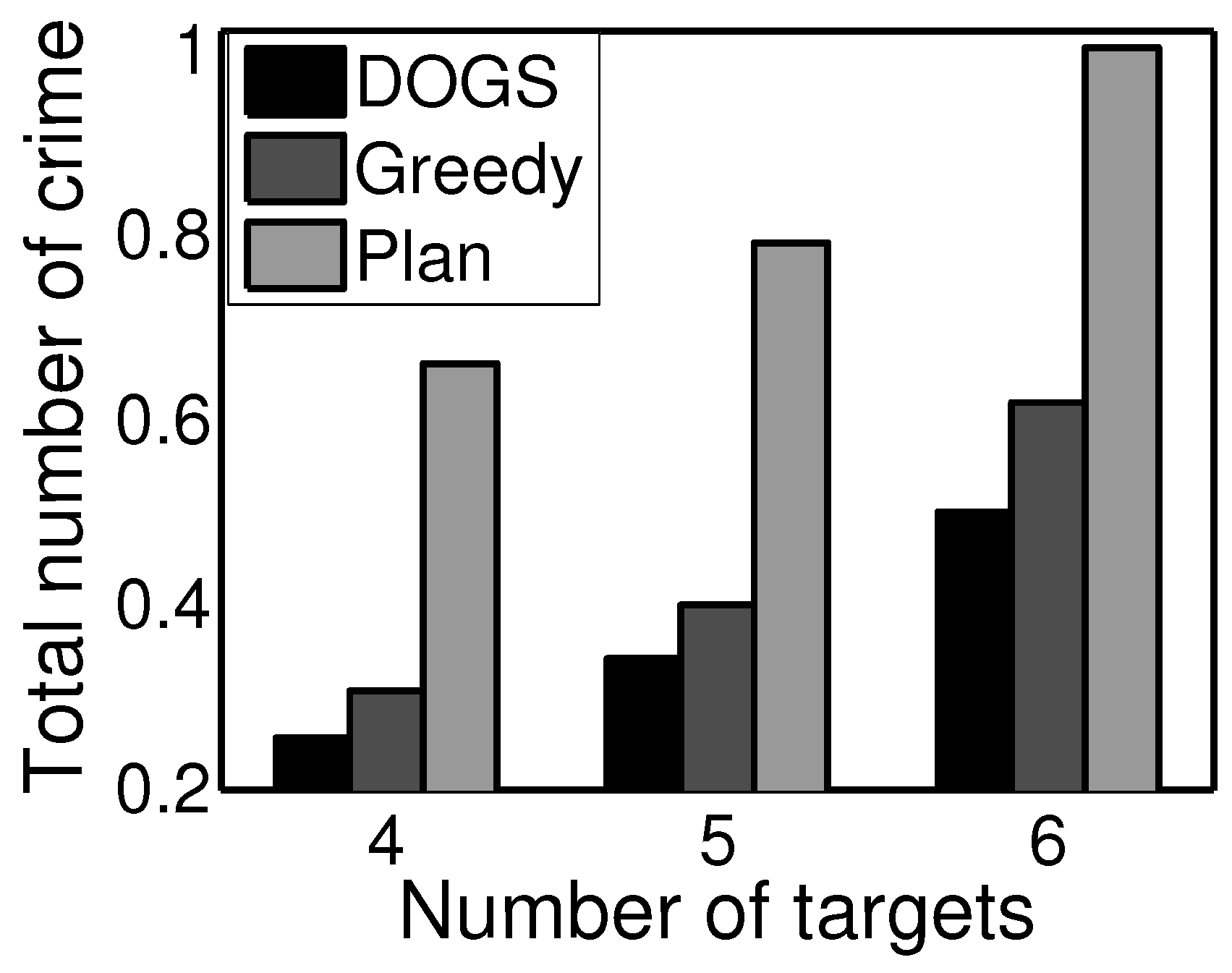
6.5. Learning and Planning Results

Figure 5g to Figure 7 present the results from our experiments about the online learning and planning mechanism. The four planning mechanisms that we consider are as follows: first, a random planning mechanism that randomly generates the allocation strategy with limited resources; second, a pure planning mechanism, where we learn the criminal behavior model once and apply this model to plan for the entire horizon T using the DOGS algorithm; third, an online planning mechanism with a greedy planning algorithm that updates every T u time steps; and the last mechanism is the online planning mechanism with the DOGS algorithm that also updates every T u time steps.
In Figure 5g, the total planning horizon T is set to 600. In addition to the four planning mechanisms, we also consider the worst case where the defender always protects the least valuable targets. The x-axis shows the update interval T u , which is the time interval after which we update the criminals’ behavior model. The y-axis is the expected number of crimes that happen under the deployed allocation strategy within 600 steps. The expected number of crimes under the pure planning mechanism stays the same with different T u , because it does not update the criminals’ model at all. For the online mechanisms, the expected number of crimes increases as the update interval T u increases. This is because with infrequent updates of the criminals’ behavior model, we cannot keep up with the real criminals’ behavior. In addition, with any size of the update interval, the DOGS algorithm outperforms the greedy algorithm. In Figure 5h, we present the runtime of three mechanisms for the same experiment. We do not show the runtime for the random planning mechanism, as it is small and the same for any planning horizon T. The runtime decreases as the update interval T u increases. There is a runtime-quality trade-off in choosing T u . Figure 7 shows the performance of the four planning mechanisms, but with different numbers of targets in the model. The x-axis is the number of targets in the graph, and the y-axis is the expected number of crimes under the deployed strategy. We set T = 600 , T u = 2 . The results here are similar to the results of Figure 5g.
These results lead us to conclude that online mechanisms outperform the baseline planning mechanisms significantly in any settings. For the online mechanisms, DOGS achieves better performance, while the greedy planning algorithm requires less runtime. Thus, based on the specific problem being solved, the appropriate algorithm must be chosen judiciously.

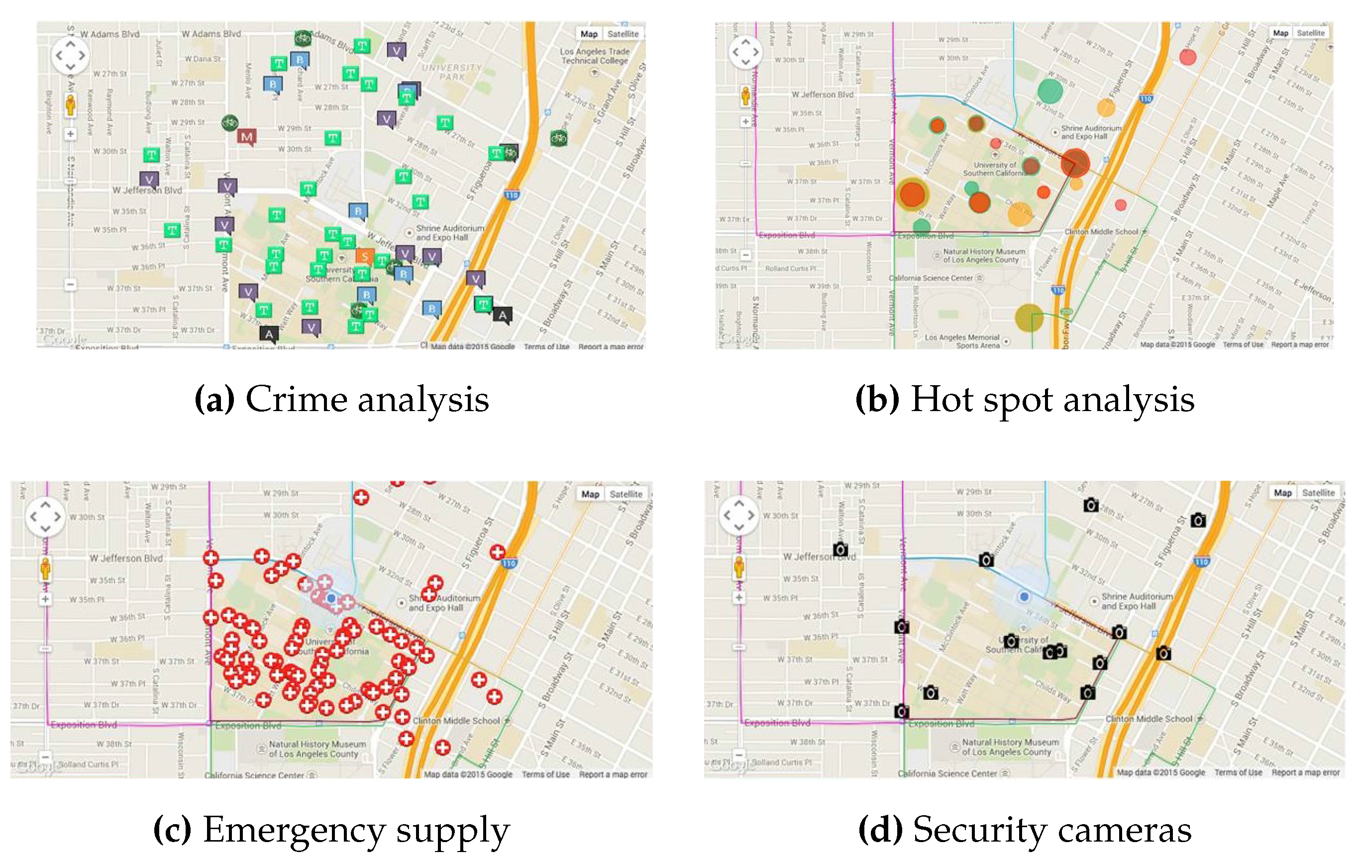
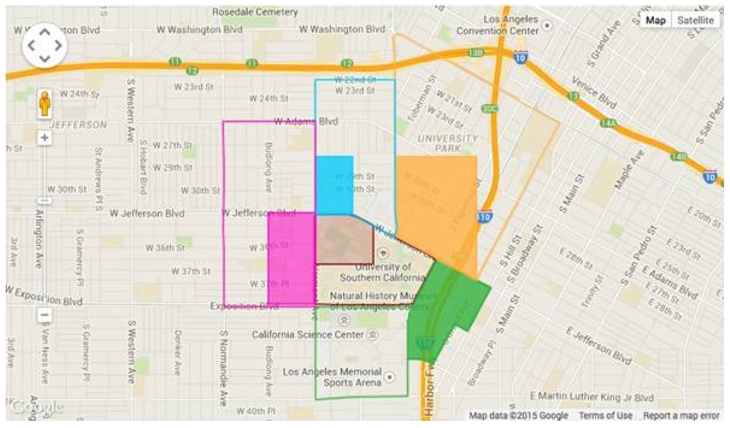
7. Real World Implementation

In this section, we introduce web-based software with two contributions. First, our system collects and analyzes crime reports and resources (security camera, emergency supplies, etc.) data, presenting them in various forms. Second, our patrol scheduler incorporates the learning and planning algorithm we proposed before in a scheduling recommendation system. The software is currently under deployment and testing at the USC campus in Los Angeles, USA.

7.1. Multi-User Software

Our multi-user web-based software is built for the Department of Public Safety at the University of Southern California. It is composed of two main components: a data collector and a patrol scheduler. A detailed demonstration of our software can be found here (https://dl.dropboxusercontent.com/ u/40377044/aamas_demo.pptx).

7.1.1. Data Collector

The data collector receives crime data from the police department and presents and analyzes them in various fashions. There are three main tasks of the data collector: First, it visualizes crime data with spatial and temporal information, as shown in Figure 8a, to help officers analyze the trend of crimes around campus. As shown in Figure 8b, ‘hot’ areas indicate attractive targets for criminals to commit crimes. As of now, the police department can cool down these hot spots by increasing patrol coverage when assigning officers in the field. However, with our planning approach, the police allocation will be more intelligent. As we also learn how criminals move in response to patrols, our approach does not simply cover the hot spots, but also allocates officers to areas where criminals are expected to move.
Second, the data collector provides information to the officers in the field about various available resources, such as emergency supplies and security cameras. As shown in Figure 8c, our software indicates the location for all of the emergency supplies on campus. Figure 8d shows the (mock) location of security cameras. To check certain locations, officers can use our software to watch the video from any camera. Finally, the data collector provides input for the patrol scheduler. By reading the data from the collector, the patrol scheduler can continuously learn and update criminals’ behavior.

7.1.2. Patrol Scheduler

Patrol settings: At USC, our approach further divides the enforcement area (encompassing the campus) into 18 patrol areas, which are shown in Figure 9. DPS patrols would be in shifts of 4 h each. At the beginning of each patrol shift, our algorithm assigns each available patrol officer to a patrol area, and the officer patrols this area in this shift.
Schedule generator: As part of the integration of our learning and planning with the software, we show the use of the EMC 2 algorithm to learn the criminals’ behavior from previous crime and patrol data and the DOGS algorithm to generate patrol schedules for DPS officers. We highlight the recommended patrol area on the campus map, as shown in Figure 10.

8. Conclusions and Future Work

This paper introduces a novel framework to design patrol allocation against adaptive opportunistic criminals. First, we use Markov chain and DBN to model the interaction between officers and adaptive opportunistic criminals. Next, we propose a sequence of modifications to the basic DBN resulting in a compact model that enables better learning accuracy and running time. Finally, we present an iterative learning and planning mechanism with two planning algorithms to keep pace with adaptive opportunistic criminals. Experimental validation with real-world data supports our choice of model and assumptions. Further, our modeling assumptions were informed by inputs from our collaborators in the DPS at USC. We project a ∼50% reduction in the crime rate using our approach as opposed to the current approach followed by DPS.
In terms of future work, we would like to capture other patterns of crime using our Markov chain and DBN, such as how crime is influenced by the time of day, day of the week, season or domain factors, such whether or not USC classes are in session or whether it is football season, and other such factors. Another line of future work would be to do a sensitivity analysis of our results by considering various divisions of the three-year real-world data available at USC. Currently, we divide the dataset into four sets of nine months each. However, comparisons and analysis of the results based on three divisions of 12 months each or other divisions based on seasons and other factors would be an interesting line of future research. yes

Acknowledgments

This research is supported by MURI grant W911NF-11-1-0332. We thank Armorway. Inc. for helping generate the software.

Author Contributions

Chao Zhang, Shahrzad Gholami, Debarun Kar, Arunesh Sinha and Milind Tambe contributed to the design of the model, ran the experiment, interpreted results and wrote the manuscript. Manish Jain and Ripple Goyal contributed to generating the multi-user software.

Conflicts of Interest

The authors declare no conflict of interest.

Appendix A

Appendix A.1. EMC 2 Procedure Initialization Step

Example 1. 
A simple way to do the initialization is to use the uniform distribution, which is:
π ( 0 , 1 ) = 0 . 5 , π ( 1 , 1 ) = 0 . 5 , π ( 0 , 2 ) = 0 . 5 , π ( 1 , 2 ) = 0 . 5 ; A ( 1 , 1 , 0 , 1 , 0 ) = 0 . 5 , A ( 1 , 1 , 0 , 1 , 1 ) = 0 . 5 , A ( 1 , 1 , 0 , 2 , 0 ) = 0 . 5 , A ( 1 , 1 , 0 , 2 , 1 ) = 0 . 5 ; . . . A ( 2 , 2 , 1 , 1 , 0 ) = 0 . 5 , A ( 2 , 2 , 1 , 1 , 1 ) = 0 . 5 , A ( 2 , 2 , 1 , 2 , 0 ) = 0 . 5 , A ( 2 , 2 , 1 , 2 , 1 ) = 0 . 5 ; B ( 1 , 1 , 1 , 0 ) = 0 . 5 , B ( 1 , 1 , 1 , 1 ) = 0 . 5 , B ( 1 , 1 , 2 , 0 ) = 0 . 5 , B ( 1 , 1 , 2 , 1 ) = 0 . 5 ; . . . B ( 2 , 2 , 0 , 0 ) = 0 . 5 , B ( 2 , 2 , 0 , 1 ) = 0 . 5 , B ( 2 , 2 , 1 , 0 ) = 0 . 5 , B ( 2 , 2 , 1 , 1 ) = 0 . 5 ;

Appendix A.2. EM C 2 Procedure Expectation Step

Forward probability:
First, we calculate P ( Y 1 , Y 2 , . . . , Y t - 1 , X i , t | D 1 , D 2 , . . . , D t - 1 ) using α ( m , k , t - 1 ) :
P ( Y 1 , Y 2 , . . . , Y t - 1 , X i , t | D 1 , D 2 , . . . , D t - 1 ) = X t - 1 P ( Y 1 , Y 2 , . . . , Y t - 1 , X t - 1 , X i , t | D 1 , D 2 , . . . , D t - 1 ) = X t - 1 P ( Y 1 , Y 2 , . . . , Y t - 1 | X i , t , X t - 1 , D 1 , D 2 , . . . , D t - 1 ) P ( X i , t | X t - 1 , D t - 1 ) P ( X t - 1 ) = X t - 1 P ( Y 1 , Y 2 , . . . , Y t - 1 | X t - 1 , D 1 , D 2 , . . . , D t - 1 ) P ( X i , t | X t - 1 , D t - 1 ) P ( X t - 1 ) = X t - 1 P ( Y 1 , Y 2 , . . . , Y t - 1 , X t - 1 , D 1 , D 2 , . . . , D t - 1 ) P ( X i , t | X t - 1 , D t - 1 ) i f   X i , t = 0 = X t - 1 m α ( m , X m , t - 1 , t - 1 ) m P ( X i , t = 0 | X m , t - 1 , D m , t - 1 ) = m X m , t - 1 α ( m , X m , t - 1 , t - 1 ) P ( X i , t = 0 | X m , t - 1 , D m , t - 1 ) i f   X i , t = 1 = X t - 1 m α ( m , X m , t - 1 , t - 1 ) [ m x i , t P ( X i , t = x i , t | X m , t - 1 , D m , t - 1 ) - m P ( X i , t = 0 | X m , t - 1 , D m , t - 1 ) ] = m X m , t - 1 α ( m , X m , t - 1 , t - 1 ) x i , t P ( X i , t = x i , t | X m , t - 1 , D m , t - 1 ) - m X m , t - 1 α ( m , X m , t - 1 , t - 1 ) P ( X i , t = 0 | X m , t - 1 , D m , t - 1 )
The complexity is this step is O ( N 2 ) to calculate the whole intermediate vector. Next, we calculate α ( i , k , t ) using P ( Y 1 , Y 2 , . . . , Y t - 1 , X i , t | D 1 , D 2 , . . . , D t - 1 ) .
α ( i , k , t ) = P ( Y 1 , Y 2 , . . . , Y t , X i , t = k | D 1 , D 2 , . . . , D t ) = X t : X i , t = k P ( Y 1 , Y 2 , . . . , Y t , X t | D 1 , D 2 , . . . , D t ) = X t : X i , t = k P ( Y 1 , Y 2 , . . . , Y t | X t , D 1 , D 2 , . . . , D t ) P ( X t | D 1 , D 2 , . . . , D t ) = X t : X i , t = k P ( Y 1 , Y 2 , . . . , Y t - 1 | X t , D 1 , D 2 , . . . , D t ) P ( Y t | X t , D 1 , D 2 , . . . , D t ) P ( X t | D 1 , D 2 , . . . , D t ) = X t : X i , t = k P ( Y 1 , Y 2 , . . . , Y t - 1 | X t , D 1 , D 2 , . . . , D t ) P ( Y t | X t , D 1 , D 2 , . . . , D t ) P ( X t | D 1 , D 2 , . . . , D t ) = X t : X i , t = k P ( Y 1 , Y 2 , . . . , Y t - 1 , X t | D 1 , D 2 , . . . , D t - 1 ) P ( Y t | X t , D t ) = X t : X i , t = k j P ( Y 1 , Y 2 , . . . , Y t - 1 , X j , t | D 1 , D 2 , . . . , D t - 1 ) j P ( Y j , t | X j , t , D j , t ) = j i X j , t P ( Y 1 , Y 2 , . . . , Y t - 1 , X j , t | D 1 , D 2 , . . . , D t - 1 ) P ( Y j , t | X j , t , D j , t ) · P ( Y 1 , Y 2 , . . . , Y t - 1 , X i , t = k | D 1 , D 2 , . . . , D t - 1 ) P ( Y i , t | X i , t = k , D i , t )
The complexity to calculate each element is O ( N ) , and the total complexity is still O ( N 2 ) .
Backward probability:
β ( i , k , t ) = P ( Y t + 1 , . . . , Y T | X i , t = k , D t , . . . , D T ) = X t + 1 P ( Y t + 1 , Y t + 2 , . . . , Y T , X t + 1 | X i , t , D t , D t + 1 , . . . , D T ) = X t + 1 P ( Y t + 1 , Y t + 2 , . . . , Y T | X t + 1 , X i , t , D t , D t + 1 , . . . , D T ) P ( X t + 1 | X i , t , D t ) = X t + 1 P ( Y t + 1 , Y t + 2 , . . . , Y T | X t + 1 , D t , D t + 1 , . . . , D T ) P ( X t + 1 | X i , t , D t ) = X t + 1 P ( Y t + 2 , . . . , Y T | X t + 1 , D t , D t + 1 , . . . , D T ) P ( Y t + 1 | X t + 1 , D t , D t + 1 , . . . , D T ) P ( X t + 1 | X i , t , D t ) = X t + 1 m ( P ( Y t + 2 , . . . , Y T | X m , t + 1 , D t , D t + 1 , . . . , D T ) P ( Y m , t + 1 | X m , t + 1 , D m , t + 1 ) P ( X m , t + 1 | X i , t , D t ) ) = m X m , t + 1 ( P ( Y t + 2 , . . . , Y T | X m , t + 1 , D t , D t + 1 , . . . , D T ) P ( Y m , t + 1 | X m , t + 1 , D m , t + 1 ) P ( X m , t + 1 | X i , t , D t ) ) = m X m , t + 1 ( β ( m , X m , t + 1 , t + 1 ) B ( m , D m , t + 1 , X m , t + 1 , Y m , t + 1 ) A ( i , D i , t , X i , t , m , X m , t + 1 ) )
This step is similar to calculating forward probability. The complexity is still O ( N ) .
Total probability:
γ ( i , k , t ) = P ( X i , t = k | Y , D ) = X t : X i , t = k P ( X t | Y , D ) = X t : X i , t = k P ( Y | X t , D ) · P ( X t , D ) P ( Y , D ) = X t : X i , t = k P ( Y 1 , . . . , Y t | X t , D ) · P ( Y t + 1 , . . . , Y T | X t , D ) · P ( X t , D ) P ( Y , D ) = X t : X i , t = k P ( Y 1 , . . . , Y t | X t , D ) · P ( Y t + 1 , . . . , Y T , X t | D ) · P ( D ) P ( Y , D ) = α ( i , k , t ) · β ( i , k , t ) j i X j , t α ( j , X j , t , t ) β ( j , X j , t , t ) · P ( D ) P ( Y , D ) = α ( i , k , t ) · β ( i , k , t ) k α ( i , k , t ) · β ( i , k , t )
In this step, we still use the transformation of the conditional probability.
Two-step probability:
ξ ( m , x m , t , i , x i , t + 1 , t ) = P ( X m , t = x m , t , X i , t + 1 = x i , t + 1 | Y , D ) = P ( Y | x m , t , x i , t + 1 , D ) · P ( x i , t + 1 | x m , t , D ) · P ( x m , t , D ) = P ( Y 1 , . . , Y t | x m , t , x i , t + 1 , D ) · P ( Y t + 1 , . . . , Y T | x m , t , x i , t + 1 , D ) · P ( x m , t , D ) P ( x i , t + 1 | x m , t ) = P ( Y 1 , . . , Y t , x m , t , D ) · P ( Y t + 1 , . . . , Y T | x i , t + 1 , D ) P ( x i , t + 1 | x m , t ) = P ( Y 1 , . . , Y t , x m , t , D ) · X t + 1 : X i , t + 1 = x i , t + 1 P ( Y t + 2 , . . . , Y T | X t + 1 , D ) P ( Y t + 1 | X t + 1 , D ) P ( x i , t + 1 | x m , t ) = P ( Y 1 , . . , Y t , x m , t , D ) · P ( X i , t + 1 | X m , t ) P ( Y t + 2 , . . . , Y T | X i , t + 1 , D ) P ( Y i , t + 1 | X i , t + 1 , D ) j i X j , t + 1 P ( Y t + 2 , . . . , Y T | X j , t + 1 , D ) P ( Y j , t + 1 | X j , t + 1 , D ) P ( X j , t + 1 | X m , t ) = α ( m , x m , t , t ) · A ( i , D i , t , X i , t , m , X m , t + 1 ) β ( j , X i , t + 1 , t + 1 ) j i X j , t + 1 ( β ( j , X j , t + 1 , t + 1 ) B ( j , D j , t + 1 , X j , t + 1 , Y j , t + 1 ) A ( i , D i , t , X i , t , j , X j , t + 1 ) )
This calculation is similar to the way we calculate γ. From the second line to the third line, we use the conditional independence of Y 1 , . . , Y t and Y t + 1 and Y t + 2 , . . . , Y T given X t , X t + 1 , D . Again, we use the normalization to represent 1 P ( Y , D ) .

References

  1. Short, M.B.; D’orsogna, M.R.; Pasour, V.B.; Tita, G.E.; Brantingham, P.J.; Bertozzi, A.L.; Chayes, L.B. A statistical model of criminal behavior. Math. Models Methods Appl. Sci. 2008, 18, 1249–1267. [Google Scholar] [CrossRef]
  2. Zhang, C.; Jiang, A.X.; Short, M.B.; Brantingham, P.J.; Tambe, M. Defending against opportunistic criminals: New game-theoretic frameworks and algorithms. In Decision and Game Theory for Security; Springer: Los Angeles, CA, USA, 2014; pp. 3–22. [Google Scholar]
  3. Jain, M.; Tsai, J.; Pita, J.; Kiekintveld, C.; Rathi, S.; Tambe, M.; Ordóñez, F. Software assistants for randomized patrol planning for the lax airport police and the federal air marshal service. Interfaces 2010, 40, 267–290. [Google Scholar] [CrossRef]
  4. Shieh, E.; An, B.; Yang, R.; Tambe, M.; Baldwin, C.; DiRenzo, J.; Maule, B.; Meyer, G. PROTECT: A deployed game theoretic system to protect the ports of the United States. In Proceedings of the 11th International Conference on Autonomous Agents and Multiagent Systems, Valencia, Spain, 4–8 June 2012; International Foundation for Autonomous Agents and Multiagent Systems: Valencia, Spain, 2012; Volume 1, pp. 13–20. [Google Scholar]
  5. Chen, H.; Chung, W.; Xu, J.J.; Wang, G.; Qin, Y.; Chau, M. Crime data mining: A general framework and some examples. Computer 2004, 37, 50–56. [Google Scholar] [CrossRef] [Green Version]
  6. Boyen, X.; Koller, D. Tractable inference for complex stochastic processes. In Proceedings of the Fourteenth Conference on Uncertainty in Artificial Intelligence, Madison, WI, USA, 24–26 July 1998; Morgan Kaufmann Publishers Inc.: San Francisco, CA, USA, 1998; pp. 33–42. [Google Scholar]
  7. Nath, S.V. Crime pattern detection using data mining. In Proceedings of the 2006 IEEE/WIC/ACM International Conference on Web Intelligence and Intelligent Agent Technology Workshops, WI-IAT 2006 Workshops, Hong Kong, China, 18–22 December 2006; IEEE: Hong Kong, China, 2006; pp. 41–44. [Google Scholar]
  8. De Bruin, J.S.; Cocx, T.K.; Kosters, W.A.; Laros, J.F.; Kok, J.N. Data mining approaches to criminal career analysis. In Sixth International Conference on Data Mining, ICDM’06, Hong Kong, China, 18–22 December 2006; IEEE: Hong Kong, China, 2006; pp. 171–177. [Google Scholar]
  9. Oatley, G.; Ewart, B.; Zeleznikow, J. Decision support systems for police: Lessons from the application of data mining techniques to soft forensic evidence. Artif. Intell. Law 2006, 14, 35–100. [Google Scholar] [CrossRef]
  10. Hespanha, J.P.; Prandini, M.; Sastry, S. Probabilistic pursuit-evasion games: A one-step nash approach. In Proceedings of the 39th IEEE Conference on Decision and Control, Sydney, NSW, Australia, 12–15 December 2000; IEEE: Sydney, NSW, Australia, 2000; Volume 3, pp. 2272–2277. [Google Scholar]
  11. Tambe, M. Security and Game Theory: Algorithms, Deployed Systems, Lessons Learned; Cambridge University Press: Cambridge, UK, 2011. [Google Scholar]
  12. Jiang, A.X.; Yin, Z.; Zhang, C.; Tambe, M.; Kraus, S. Game-theoretic randomization for security patrolling with dynamic execution uncertainty. In Proceedings of the 2013 International Conference on Autonomous Agents and Multi-Agent Systems, Saint Paul, MN, USA, 6–10 May 2013; International Foundation for Autonomous Agents and Multiagent Systems: Saint Paul, MN, USA, 2013; pp. 207–214. [Google Scholar]
  13. Yang, R.; Ford, B.; Tambe, M.; Lemieux, A. Adaptive resource allocation for wildlife protection against illegal poachers. In Proceedings of the 2014 International Conference on Autonomous Agents and Multi-Agent Systems, Paris, France, 5–9 May 2014; International Foundation for Autonomous Agents and Multiagent Systems: Paris, France, 2014; pp. 453–460. [Google Scholar]
  14. Basilico, N.; Gatti, N.; Amigoni, F. Leader-follower strategies for robotic patrolling in environments with arbitrary topologies. In Proceedings of the 8th International Conference on Autonomous Agents and Multiagent Systems, Budapest, Hungary, 10–15 May 2009; International Foundation for Autonomous Agents and Multiagent Systems: Budapest, Hungary, 2009; Volume 1, pp. 57–64. [Google Scholar]
  15. Basilico, N.; Gatti, N.; Rossi, T.; Ceppi, S.; Amigoni, F. Extending algorithms for mobile robot patrolling in the presence of adversaries to more realistic settings. In Proceedings of the 2009 IEEE/WIC/ACM International Joint Conference on Web Intelligence and Intelligent Agent Technology, Milan, Italy, 15–18 September 2009; IEEE Computer Society: Washington, DC, USA, 2009; Volume 2, pp. 557–564. [Google Scholar]
  16. Blum, A.; Haghtalab, N.; Procaccia, A.D. Learning optimal commitment to overcome insecurity. In Proceedings of the 28th Annual Conference on Neural Information Processing Systems (NIPS), Montreal, QC, Canada, 8–13 December 2014.
  17. Malik, A.; Maciejewski, R.; Towers, S.; McCullough, S.; Ebert, D.S. Proactive spatiotemporal resource allocation and predictive visual analytics for community policing and law enforcement. Vis. Comput. Graph. 2014, 20, 1863–1872. [Google Scholar] [CrossRef] [PubMed]
  18. Dempster, A.P.; Laird, N.M.; Rubin, D.B. Maximum likelihood from incomplete data via the EM algorithm. J. R. Stat. Soc. Ser. B (Methodol.) 1977, 39, 1–38. [Google Scholar]
  19. Bishop, C.M. Pattern Recognition and Machine Learning (Information Science and Statistics); Springer-Verlag New York, Inc.: Secaucus, NJ, USA, 2006. [Google Scholar]
  20. Blumer, A.; Ehrenfeucht, A.; Haussler, D.; Warmuth, M.K. Occam’s Razor. Inf. Process. Lett. 1987, 24, 377–380. [Google Scholar] [CrossRef]
  21. Aji, S.M.; McEliece, R.J. The generalized distributive law. IEEE Trans. Inf. Theory 2000, 46, 325–343. [Google Scholar] [CrossRef]
Figure 1. Campus map.
Games 07 00015 g001
Figure 2. Sample data for (a) crime and (b) patrol respectively.
Games 07 00015 g002
Figure 3. Markov chain model (MCM) structures.
Games 07 00015 g003
Figure 4. The Dynamic Bayesian Network (DBN) for games.
Games 07 00015 g004
Figure 5. Experimental results.
Games 07 00015 g005
Figure 6. Markov chain models.
Games 07 00015 g006
Figure 7. Varying N.
Games 07 00015 g007
Figure 8. Data collector.
Games 07 00015 g008
Figure 9. Patrol area.
Games 07 00015 g009
Figure 10. Sample patrol schedule.
Games 07 00015 g010
Table 1. Crime data for 3 shifts.
ShiftABCDE
111222
211121
321131
Table 2. Patrol data for 3 shifts.
ShiftABCDE
121111
211222
321131

