1. Introduction
Cost allocation is the process of dividing the costs of a multi-purpose or a multi-agent project among the various project purposes or beneficiaries. Criteria and principles used for cost allocation are decided at the planning phase of the project and can lead to a situation where some of the beneficiaries are unsatisfied and thus the project may fail. Some of the cost allocation schemes are based on simple rules, proportional to a single parameter, which can lead to allocation solutions that are not acceptable by all participants. This is especially true when the affordability of beneficiaries to share the cost widely varies, or when beneficiaries face different conditions affecting their ability to benefit from the project. This paper demonstrates the application of Cooperative Game Theory (CGT) to an irrigation project that has been considered for implementation in the West of the Nile Delta in Egypt.
The main issues to which CGT tries to address are agreements to allocate joint gains, using solution concepts. Solution concepts are rules of allocation of gains from cooperation that the cooperating members of a given group can share. The number of allocation solution concepts is quite large, due also to the diversity of the problems that CGT can address. A review of the literature of CGT cost and benefit allocations in water projects can be found in [
1]. Among the most known solutions are: the Core, the Shapley Value [
2], and the nucleolus [
3]. For a general introduction to game theory and in particular to cooperative games see [
4,
5,
6]. The Shapley value, in particular, has been successively used as a cost allocation method in many applications (see, for instance, the survey [
7]), including the management of environmental resources (e.g., see [
8]).
In most of its solution approaches, CGT ignores the strategic stages leading to coalition building and focuses on the possible results of cooperation. CGT attempts to answer questions such as which coalitions can be formed? How can the coalitional gains be divided in order to secure a sustainable agreement? Often, for joint projects, the optimal way to maximize the gains (revenues minus costs, or cost savings) is to build a facility (for example) that involves all of the interested players. Thus, in CGT, the solutions that include all possible players (Grand Coalition) are prominent, and thus most CGT solution concepts refer to a way of allocating among players the gains achieved by the Grand Coalition. As such, CGT is a good framework for allocation of joint costs or benefits among participants in a project.
An important aspect associated with the solution concepts of CGT is the
equitable and fair sharing of the cooperative gains. One can refer to equity in a comprehensive framework, that is, social justice—a proper distribution of resources, welfare, rights, duties, opportunities, or in our case the costs of an investment and of Operations and Maintenance (O&M) of a project. There have been many applications of CGT to allocation issues in water projects, including the publication [
9]. In most, if not all previous works, simplifications of the allocation problem have been introduced, which made the application less operational.
In this paper, we introduce an application of cooperative game theory to a cost allocation problem arising from a complex water project in Egypt, taking into account differences in the regional landscape of land sectors (sectors) of the project area that affect the benefits that can be accrued by water users in each of the project land sectors. We demonstrate the challenges faced during the application of cooperative game theory concepts and how they are addressed. The analysis produces a differential two-part tariff that differs by the project land sectors, in contrast to the unified tariff that was recommended by the traditional methods used by the planners.
We start in the next section with some basic definitions and notations on cooperative games.
Section 3 is devoted to the description of the analytical framework related to the West Delta Project (WDP). In
Section 4, we introduce and discuss the data and the procedures used to evaluate the relevant costs and the revenues under two different scenarios of water supply, namely, alternative A0 and A2. In
Section 5 and
Section 6, we describe how we computed the (cost and revenues) cooperative games associated with scenarios A2 and A0, respectively. The cooperative games defined in
Section 5 and
Section 6 are compared and discussed in
Section 7, together with the analysis of the associated cost allocation problem.
Section 8 concludes this paper.
2. Preliminaries and Notations
A cooperative cost game (or, simply, a cost game) on a finite set of players is a pair where the characteristic function c is a map assigning to each coalition a real value representing the cost of coalition S, and with . A cost game is subadditive if for all such that .
Given a cost game , an imputation is a vector such that and for each . An imputation is in the core of the cost game if for all .
A very well studied solution from the literature of cooperative games is the
Shapley value (Shapley 1953, [
2]), which is defined for every cost game
as follows:
where
s is the cardinality of a coalition
S and
is the
marginal contribution of
to
for each
and
. Thus,
is the expected marginal contribution of player
in the cost game
over all possible coalitions not containing
and assuming that the probability to enter in a coalition of size
s is equal to
. The Shapley value
of a subadditive cost game
is an imputation of
, but
is not necessarily in the core of
. A sufficient condition to have
in the core of
is that
is
submodular or
concave, i.e.,
for all
.
3. The Analytical Framework
As an example, tailored to the West Delta Project (WDP) scheme presented below, of a cooperative game, considers a three-player game, whose players are 1, 2, and 3
1. Each player faces a different physical situation that affects his performance (costs and benefits). Assume that the players want to build a system of irrigation infrastructure to be used by all of them for production. The presence of joint costs will require some way of attributing them to each player. One way of allocating joint costs is to apply approaches used in cooperative game theory. The idea is quite simple in principle. One has to find what would be the costs if the infrastructure would be built just for one player (singleton coalitions). Then do the same for each group of two players (partial coalitions), and finally, for the entire group (grand coalition) of the three players. In such a way one gets a string of numbers (costs), that we shall call
c(1),
c(2),
c(3),
c(1,2),
c(1,3),
c(2,3) and, of course,
c(1,2,3) (the later is the cost of the project as appears in the project documents). This is a cooperative (cost) game, and one looks for “allocation solutions” to this game; namely, how to allocate the project cost among 1, 2, and 3. In general, a solution is assumed to be an imputation. That is, it will share exactly the total joint cost among the players, without attributing to anyone a cost higher than its “stand-alone” cost,
c(
i),
i = 1, 2, 3 in our case. In our model, we will develop a cooperative cost game to see the feasibility and interest of all the players in the construction of the surface irrigation system. We use the Shapley Value to allocate the costs among the players.
While the project documents suggest a certain tariff to be charged to the players, we have investigated which would be the tariff (or the tariffs) proposed by the cooperative game theory analysis. We will develop a cooperative cost game to analyze the feasibility of different methods for sharing the costs for building the surface irrigation infrastructure, using the Shapley Value. We develop a cooperative cost game to see the feasibility and interest of all the players in the construction of the surface irrigation system. Finally, based on the cooperative game, we find out which operational two-part tariff for surface water could be used to reproduce the fair solution (which is, in our case, the Shapley Value). The challenge, of course, is the setting of various characteristic functions, which is the focus of this paper.
3.1. Features of the West Delta Water Conservation and Irrigation Rehabilitation Project
The West Delta Water Conservation and Irrigation Rehabilitation Project (WDP) was a unique attempt of the Government of Egypt to prevent the environmental degradation of the flourishing West Delta region. The massive agriculture development of the region (about 107,000 ha) led to depletion and salinization (seawater intrusion) of groundwater resources. The project is based on the premise that supplementing the groundwater in the region with imported Nile water to irrigate the existing land and even extending it, can be done in both an ecologically and financially sustainable way. An innovative component of the project was the inclusion of a for-profit private sector entrepreneurship that will fund the investment, manage the cost recovery, and operate the surface irrigation system according to specified rules of operation. Another innovative component was the introduction of full cost recovery and volumetric pricing. The Government of Egypt was supposed to provide guarantees to mitigate financial risks faced by the private entrepreneur from non-payments by farmers in the project. Eighty five percent of the cost of the first phase of the project (about 38,000 ha) was supposed to be funded by the World Bank ($145 million) and the French Development Agency (EUR 30 million). The other 15% of the first phase cost and the cost of the next phases had to be raised by the private operator. More information on the project and its closure can be found in [
12].
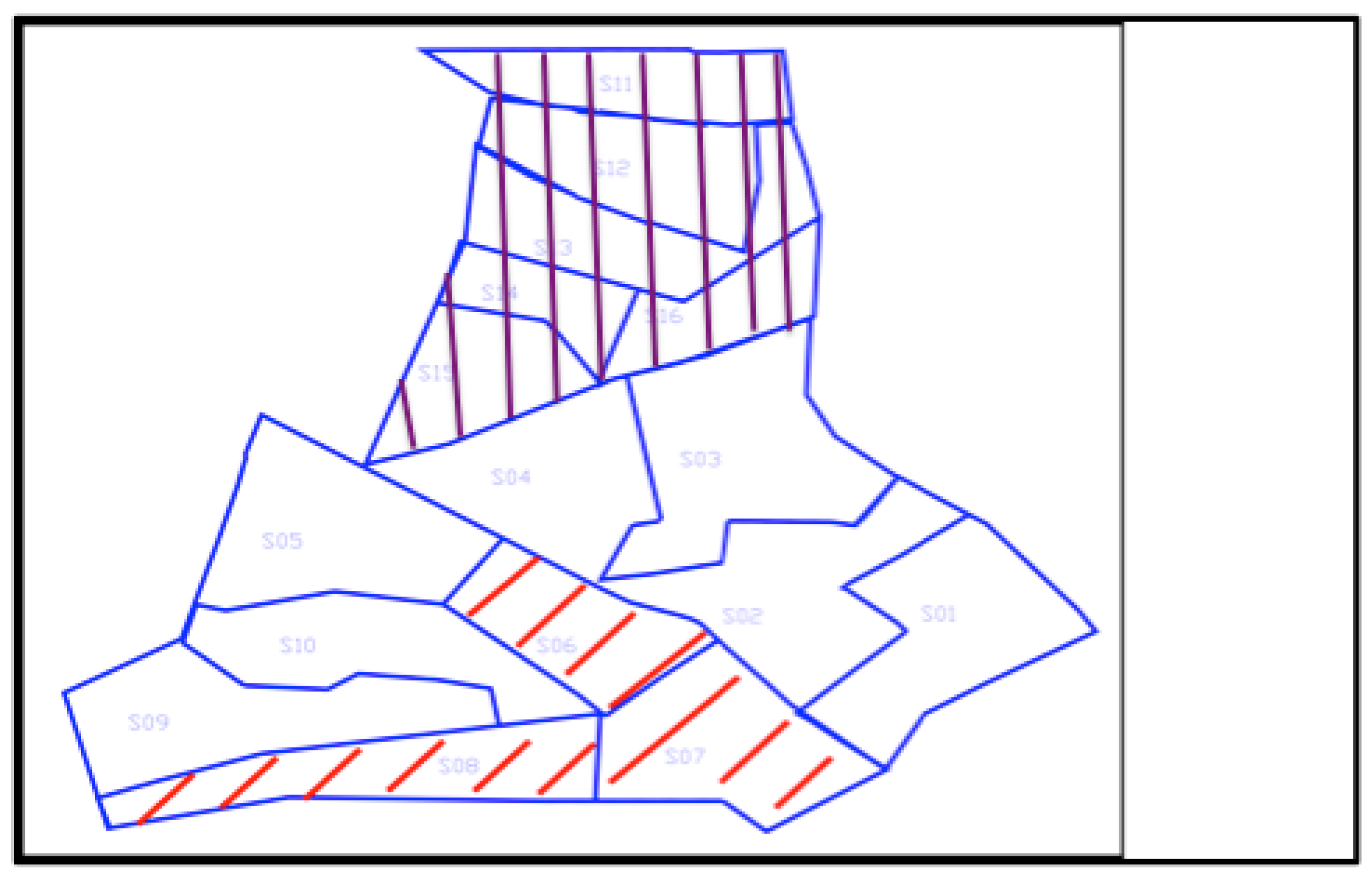
The most critical question related to the project was how to design the cost recovery scheme that will fully cover all costs, will be acceptable to the various users (farmers), and at the same time will be attractive to a private investor. The reason for that can be seen in the map of the region below (
Figure 1). The project area can be divided into three distinguished sectors: Central (player 1), Southern (player 2) and Northern (player 3). The three sectors differ in both their size of land holding, and in the (average) depth to water table (i.e., the depth at which the ground beneath the surface is saturated with water)
2. Sectors’ size will affect the investment cost per unit of land due to economies of scale and pumping cost. Sectors’ depth to water table will affect the cost of pumping groundwater and, thus, the willingness to pay for imported surface Nile water (
Table 1).
The cost
3 per player will affect the profit level and, therefore, the willingness to participate in the project and contribute to the cost recovery, which is a fundamental condition for the risk a private investor may be willing to take.
3.2. The Empirical Framework
In this model we consider three
players, each one is formed by a subset of land owned by farmers in various sectors of the project (
Figure 1). We assume that all farmers in each sector, or sub-region, can be represented by one voice.
Player 1,
central region, consists of sectors {S01, S02, S03, S04, S05, S09};
player 2,
southern region, consists of sectors {S06, S07, S08}; and
player 3,
northern region, consists of sectors {S11, S12, S13, S14, S15, S16}. This choice of sectors and sub-regions for the players is very close to the situation of
Market and Demand Parameters (MDP) project option for alternative A2
4 (PPIAF, 2005 [
14]). Therefore, our cost allocation game is based on three players/regions characterized by different size of land and depth to groundwater table as shown in
Table 1 5.
4. Description of the Data and Procedures Used
This section describes the various types of costs and revenues that are considered under the two alternatives scenarios of water supply to the project: A0 and A2. All the data used in our analysis originated from several reports prepared by the World Bank [
12,
15] and several local and international consultants [
13,
14,
16,
17,
18]. Since the project is funded mainly by the World Bank, it has to follow the World Bank procedures. As such, [
13,
14,
16,
17,
18] are reports that prepared the project design and different assessments (e.g., irrigation efficiency, net benefits and their distribution across beneficiaries, soil and groundwater quality, environmental and social assessment, and public–private partnership performance and risk—the private sector had a major role in this project). The report [
15] is the project appraisal report, which is based on the reports cited above and a series of discussions with the Government of Egypt. This report triggered the approval of the project and the initiation of the procedures in the project plan. The [
12] report addresses the termination of the project.
Under both alternatives,
investment costs for irrigation equipment are considered for a time period of 20 years, and
running costs (O&M and labor) are considered on a per-year basis. Yearly revenues have been calculated on the basis of the cropping patterns derived from the farm survey results (Annex 1 and 3 in [
13]). Net benefits are calculated, based on an optimal allocation of land use for irrigated crops in each sub-region [
13]. When the net benefits from irrigated agriculture under Alternative A0 (business as usual) turn negative due to high level of salinity, the reference cropping pattern is replaced by a more salt tolerant (and less profitable) cropping pattern. This switch consists primarily on a different allocation of the area for crops (e.g., an increase in the area cultivated with grapes, which has been supposed to double after Year 13).
Under alternative A0, it has been evaluated that after 13 years from the first year of connection to surface water the loss in agricultural production in the Nile Delta would make it more profitable for farmers to leave the project area. Consequently, alternative A0 has been considered to produce revenues for only 13 years. The main assumptions, sources of data, etc. used in the financial part of the model, are presented in Annex 3 of the WDWCIARP Drainframe Analysis, Main Report [
13]. The chosen time period is 13 years, starting from the first year of connection to surface water. This rather short timeframe has been chosen in order to provide consistent results for the different evaluated impacts. This is also the timeframe of the National Water Resources Plan (NWRP); therefore, we adopted a financial model with a similar time horizon. Extending the timeframe by 20–30 years would show even more clearly that the impacts on agricultural production under A0 are unsustainable.
4.1. Scenario A2
Scenario A2 considers no groundwater use. Thus the capacity of the conveyance system should be designed to meet the peak monthly surface water requirement of 222 million cubic meters in June, [
14].
Under scenario A2, we have considered the investment costs categories reported in
Table A1 in
Appendix (from [
13]) and the running cost (O&M) shown in
Table A2 in the
Appendix (based on [
16]).
For alternative A2, a reference crop pattern is reported in
Table 2. It consists of high value crops with a higher share of perennial trees (79%) and vegetables (21%). Under A2, where the surface irrigation system is designed in order to meet peak summer requirements, it is assumed that farmers will maintain the current cropping pattern.
For summer and winter vegetables, double cropping has been assumed in a six-month periods for both summer and winter crops under the reference cropping pattern only. Revenues from production of different cropping patterns are assumed to depend on the expected yields according to Mass-Hofman formula [
19]. This means that under this alternative they depend on the average soil salinity under Nile water irrigation.
4.2. Scenario A0
Scenario A0 represents the case of continued dependence on ground water only (business as usual).
Under scenario A0, we have considered the investment costs categories shown in
Table A3 in the
Appendix (based on [
16]) and the running cost categories reported in
Table A4 in the
Appendix (based on [
16]).
Under scenario A0, the reference cropping pattern is assumed to be the same as in A2 (
Table 2). For summer and winter vegetables, double cropping has been assumed in a six-month periods for both summer and winter crops of the reference cropping pattern only. It is also assumed in A0 that farmers will continue to grow the reference cropping pattern as long as the net benefits remain positive. More precisely, after Year 13, the model yields negative benefits and it is assumed that the (less sensitive to water salinity) cropping pattern shown in
Table 2 is adopted. The switch consists primarily in a different allocation of the area for each crop (i.e., a relative increase in the area cultivated with grapes), while only in one case a particularly salt sensitive crop (pear) is replaced by a more tolerant one (maize). Moreover, we assume that at the Year 15, after the intense use of water during the previous years, the yield of the crop pattern in
Table 2 would be at 80% of the saline non-stressed fields.
Revenues from production of the two different crops are assumed to depend on the expected yields [
13], and hence ultimately on the expected behavior of groundwater salinity [
16]. When the switch to cropping pattern in
Table 2 occurs, we considered a single cropping for vegetables and a 20% of yield reduction with regards to the non-stress situation for the other products in
Table 2 (grapes and other crops).
5. Assigning the Investment and Running Costs and the Revenues to the Various Coalitions in the Game under Alternative A2
We use the existing cost items provided by in the World Bank project document [
15]. Our goal is to assign costs to each possible coalition, i.e., each possible sub-group of the three land sections. Since the project documents [
15] were prepared to estimate the cost of implementation on the overall area (grand coalition consideration), we developed a methodology for assessing the costs for the intermediate coalitions. We used the cost data on investment and running cost items related to the project. For certain items the information is provided for the entire project, and for some items data is aggregated for land sectors and yet for some other cost items the data is provided for each individual sector (see
Figure 1 and first paragraph of the Empirical Framework Section).
According to this information and assuming equal distribution of cost per hectare among all land blocks we used the available information to estimate the cost of coalitions in three different cost games as explained in more detail in the next section. The resulting cost allocations of investments and running costs per region (that were used below to create the cost per coalition) can be found in an excel file that is provided in the auxiliary dataset to this paper [9]. In the following, we describe how we estimated the amount of investment costs for each coalition of players.
Finally, in the last part of this section (namely, in
Section 5.3), we introduce the procedure used to determine the revenues of each coalition under alternative A2 on the basis of the information provided in [
14] and [
13,
16,
17].
5.1. Evaluation of the Investment Costs under Alternative A2
To determine our cost game, we shall consider it as the sum of three games, c
A2,1, c
A2,2 and c
A2,3. This decomposition into three different cost games is based on our ability to apportion the various costs from available data [
20,
21] to the various coalitions.
In game c
A2,1, only the cost of the grand coalition {1,2,3} can be directly assessed. In game c
A2,2, only the costs of coalitions {1,2},{3} and {1,2,3} can be assessed directly, and, in game c
A2,3, the costs of all coalitions are assessed from the available data
6. All three games are used in the calculation of the Shapley Value. We use all three games to produce the cost of all seven coalition-sections in the project area. Both c
A2,1 and c
A2,3 are additive cost games. c
A2,1 is calculated starting from the value of the grand coalition (taken from the costs presented in [
21]), and then proportionally allocated by the area of each sub-coalition (See footnote 6). c
A2,3 is also additive but the cost items in this game are a priori assigned to the three section in the data taken from [
15], so the cost of each larger coalition is computed additively based on these data. In the following discussions and tables, all costs have been considered in 10
6 LE (Egyptian Pounds)
7.
5.1.1. Costs Items in Game cA2,1
Costs considered in game c
A2,1 are the following (
Table 3).
5.1.2. Cost Items in Game cA2,2
Costs considered in game c
A2,2 are presented in
Table 4.
The cost in
Table 4 allow us to assess the total amount, for coalitions {1,2}, {3} and {1,2,3}, as c
A2,2(1,2) = 599.941; c
A2,2(3) = 176.796; and c
A2,2(1,2,3) = c
A2,2(1,2) + c
A2,2(3) = 776.737, respectively.
5.1.3. Costs in Game cA2,3
Costs considered in game c
A2,2 are presented in
Table 5. All costs considered here concern components that can be directly attributed to each region in
Figure 1. The resulting cost game is an additive game, that is, the cost for coalition
S ⊆ {1, 2, 3} is equal to the sum of the individual costs for players in coalition
S. Note that these kinds of costs correspond to those cost components of the project which can be directly allocated to each participant.
The resulting additive cost game ({1,2,3},c
A2,3) is presented in
Table 6.
5.1.4. Missing cost Estimation for Intermediate Coalitions
In
Section 5.1.4.1 and
Section 5.1.4.2, we present how we estimated the value of coalitions in games c
A2,1 and c
A2,2, whose costs were not possible to be evaluated from the data spreadsheet in the project documents [
13,
14,
20].
5.1.4.1. Estimation of the Cost of Intermediate Coalitions in Game cA2,1
Costs of intermediate coalitions have been estimated in game cA2,1 proportionally to the area of the corresponding region covered by the coalition. For example, for coalition {1,2}, the cost assigned to such coalition has been estimated as the fraction (area of central and southern region)/(area of the entire region) of the total cost evaluated from the spreadsheet for the entire region c({1,2,3}). Of course the assumption of direct proportionality produces a rough approximation of the costs for each coalition, but it is needed to address the lack of information in the project documents.
5.1.4.2. Estimation of the Cost of Intermediate Coalitions in Game cA2,2
This case, which is directly assessable from the spreadsheet, is the cost for two distinct regions, region {1,2} and region {3}. The main characteristics affecting the value of these costs have been assumed to be the water intake that is assumed to be proportional to the dimension of the served area. A secondary variable, which has been assumed to affect the costs considered in this game is the average depth to water table of the served lands.
Therefore, we considered a model for cost estimation where costs are mainly function of the area of the served regions plus another term representing the interaction between the area and the average level of the regions served. In formula, we considered the model
where
F is the size of the served area (Feddan),
H is the average depth to water table of the served area (meter),
a and
b are coefficients,
K is a fixed cost component, and
C is the total cost for cost items presented in
Table 4 and analyzed in game c
A2,2. Note that the parameter
F for a coalition S has been calculated as the sum of the area (in Feddan) of players in S, whereas the parameter
H has been obtained as a weighted average of depth to water table for players in
S. For example, if S = {1,2}, then
F(S) = (141,600 + 48,400) = 190,000 Feddan and
H(S) = (141,600 × 85 + 48,400 × 110)/(141,600 + 48,400) = 91.37 m.
Fitting the model in Equation (2) to data presented in
Section 5.1.2, the resulting optimal coefficients are
a = 0.002,
b = 9.43844 × 10
6 and
K = 0 and the corresponding costs for game c
A2,2 are shown in
Table 7.
5.1.5. Total Investment Costs Game under Alternative A2
Summing up, the cost games related to the investment costs under alternative A2 are shown in
Table 8 (costs in 10
6 LE), where ({1,2,3},c
A2(S)) is the total investment cost game under alternative A2.
The game cA2(S)/20 is the amount of investment cost that should be supported each year by the corresponding coalitions under alternative A2, in an ideal situation where the principal amount can be amortized over 20 years.
Next, we consider a situation with a more accurate estimation of the effects of time on the cash flows.
5.2. Evaluation of Running Costs under Alternative A2
Running costs (O&M) are costs that farmers should support every year for operating and maintaining all the agriculture procedures. Similar to what was observed for investment cost, we observed three different kind of running cost games, the games r
A2,1, r
A2,2 and r
A2,3, again different from each other by the possibility to assess the cost of each coalition of players directly from data presented in [
20]. In game r
A2,1, only the cost of the grand coalition {1,2,3} is directly assessed. In game r
A2,2, only the costs of the coalitions {1,2},{3} and {1,2,3} are directly assessed and, in game r
A2,3, the costs of all the coalitions are assessed, from direct attribution of costs presented for the regions depicted in
Figure 1.
5.2.1. Costs in Game rA2,1
Costs considered in game r
A2,1 are the following (
Table 9).
For costs in
Table 9 it is possible to assess the total amount, for the grand coalition, that is r
A2,1 = 60.691.
5.2.2. Costs in Game rA2,2
Costs considered in game rA2,2 are the following.
For costs in
Table 10 it is possible to assess the total amount for coalitions {1,2}, {3} and {1,2,3}, precisely as r
A2,2(1,2) = 60.06; r
A2,2(3) = 11.5; and r
A2,2(1,2,3) = r
A2,2(1,2) + r
A2,2(3) = 71.56, respectively.
5.2.3. Costs in Game rA2,3
Costs considered in game r
A2,3 correspond to Sub Mains Boosters costs (see
Table A1 in
Appendix for a short description of the cost categories). All costs considered here concern those components that can be directly attributed to each area in
Figure 1. The resulting cost game is an additive game. The total cost for the entire area is 767.888 × 10
6 LE.
The resulting game ({1,2,3},r
A2,3) is presented in
Table 11.
5.2.4. Cost Estimation for Intermediate Coalitions
As for the investment costs, costs of intermediate coalitions in game rA2,1 have been assumed to be directly proportional to the area of each region.
Estimation of Game rA2,2
For running costs, where the cost of energy employed for the operations is the main variable that affects the costs considered in
Section 5.2.2, we assumed that both land area and average level have the same weight in the model for cost estimation. For this reason, we assumed the following model for running cost estimation
where
C′ is the total cost for cost items presented in the
Section 5.2.2,
F′ is the extension of the area served (Feddan),
H′ is the average level of depth to water table in the area (meter),
a′ is coefficient which represents the variable cost component and
K′ is the fixed component for running costs. Fitting the model in relation (3) to data presented in
Section 5.2.2, the resulting optimal coefficients are
a′ = 0.003457258 × 10
−3 and
K′ = 1.393520161, and the corresponding game r
A2,2 has the characteristic function shown in
Table 12.
5.2.5. Evaluation of Labor Cost and Production rlp
Cost of seasonal labor is assumed to depend both on the total cultivated area (70% weight) and on the level of production (30% weight), while permanent labor is assumed to only depend on the cultivated area. These coefficients and assumptions are based on [
16]. Other costs of production (seeds, fertilizers, machinery, etc.) are reported on a per Feddan basis, taking into account the reference cropping pattern [
16]. Resulted costs appear in
Table 13 and
Table 14.
The reference-cropping pattern considered is the one shown in
Table 2. The total area is 255,000 Feddan. Given these parameters, the aggregated
labor and
production cost game r
lp is shown in
Table 15. Note that the cost estimation for labor and production has been done to provide a holistic picture in the project area only because the allocation problem for these costs is clearly defined: each individual farm will support its own costs of labor and production.
5.2.6. Total Running Cost Game under Alternative A2
Summing up, the cost games related to the running costs (on a per year basis) under alternative A2 are shown in the following table (106 LE), where rA2(S) is the total running cost game under alternative A2.
5.3. Revenue Evaluation under the Alternative A2
Under this alternative the cultivated area is assumed to reach the full area of 255,000 Feddan. Unit revenues from production of different crops are reported in
Table 16.
Under alternative A2 (no use of groundwater), we assume that the salinity of (Nile) water has been assumed to remain constant over the entire period of 20 years, which has been considered in this analysis [
13,
14,
16,
17]. According to [
13,
16,
17], the revenues from production of different crops are assumed to depend on the expected yields and, ultimately, on the expected behavior of groundwater salinity under alternative A2. Therefore, yields, costs and profits remain constant over time under alternative A2.
Summing up, the revenue game ({1,2,3},v
A2), which provides the revenue of each coalition under alternative A2, is shown in
Table 17.
6. Assigning the Investment and Running Costs and the Revenues to the Various Coalitions in the Game under Alternative A0
In this section, we use again World Bank project document [
14,
15] and the same approach previously introduced in the previous section to assign costs and revenues to each possible sub-group of the three land areas under alternative A0.
6.1. Investment Cost Evaluation under the Alternative A0
Investment costs in irrigation equipment include groundwater pumping equipment (wells, pumps, engines, and fuel tank) and the cost of the irrigation system (drip lines, hydrants, etc.). The assumed average lifetime of these elements for A0, where the ground water (GW) pumping equipment has a relatively short life expectancy, is the following: 10 years for well, pump and engine, 30 years for fuel tank [
17]. The cost of this equipment is reported in
Table 18.
As shown in
Table 18, the size of the needed equipment depends on the size of the area served. Thus, the investment cost game ({1,2,3},c
A0) under alternative A0 is depicted in
Table 19.
6.2. Running Cost Evaluation under the Alternative A0
Running costs incorporate O&M costs, labor costs, production costs and energy costs. O&M costs have been assumed equal to 5% of the yearly investment in equipment. Costs of supply of irrigation water include energy costs for water pumping. Energy cost per unit water has been estimated in [
16] to be 0.029 LE/m
3. The annual water requirement for a reference-cropping pattern for 100 Feddan has been than estimated at about 6250 m
3/year.
Cost of labor and production per year have been calculated according to cost values shown in
Table 13 and
Table 14, with respect to the cultivated area under alternative A0. As we already indicated, the cost allocation for labor and production is already allocated (each farm will pay its own cost of labor and production cost) but it is included in the calculation to provide a more detailed account of all costs. The running cost game ({1,2,3},r
A0) is then the one depicted in
Table 20.
6.3. Revenue Evaluation under the Alternative A0
This alternative assumes continued use of groundwater, which is deteriorated in quality over time. The reference-cropping pattern is reported in
Table 2. For this cropping pattern only, for summer and winter vegetables double cropping has been assumed in six-month periods for both summer and winter crops. Under alternative A0 the cultivated area is assumed to reach the partial area of 123,848 Feddan. After Year 13, the reference-cropping pattern has been substituted by the cropping pattern in
Table 2.
Under alternative A0 the effect of salinity of irrigation water on yields is determined following the methodology reported in the economic model in the Annex 3 of [
16], with the effect of salinity on yields being calculated according to the formula [
19]:
where
Y(t) is the absolute yield,
A is threshold salinity at which a crop start to suffer from salinity (dS/m),
B is rate of yield decrease % per dS/m increase in salinity,
ECe(t) is mean electrical conductivity of saturated paste of the soil in (dS/m) at time
t, and
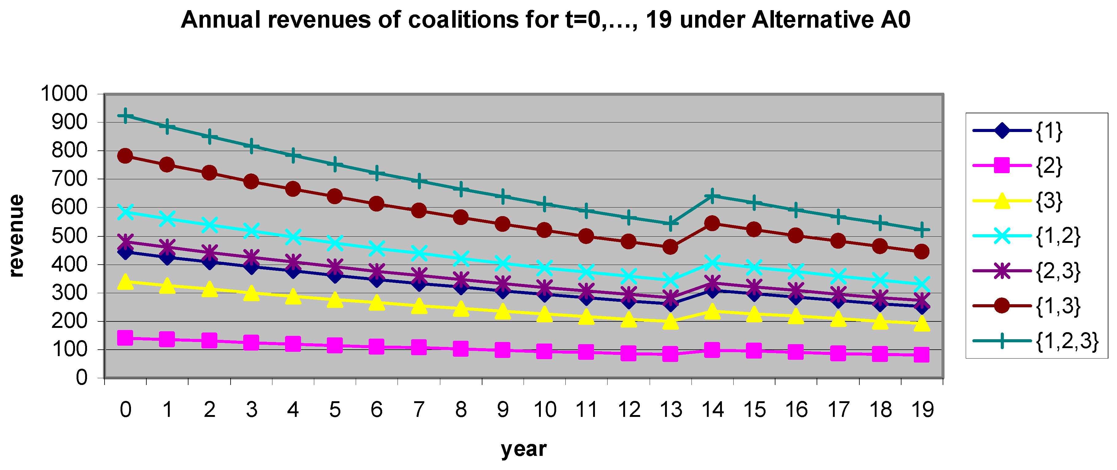
Yns is the non stress yield level (ton/Feddan). Consequently, each year, each coalition gets an incremental decrease of its revenues of about 4%. All revenue games are shown in the
Table A5.
Therefore, and due to the annual decrease of revenues, we face 20 revenue games v
tA0, where
t = 0, 1, …, 19 is the year index. All revenue games shown in
Table A5 are also depicted in
Figure 2. It has been shown in the simulation presented by [
16] that after Year 13, alternative A0 produces a negative net benefit under the reference-cropping pattern. Because of these negative net benefits, farmers are supposed to switch the cropping pattern in
Table 4 (Scenario A0) to the one in
Table 2 (Scenario A2), which yields the revenues reported in italics in
Table A5.
7. Game Comparison for Alternatives A0 and A2
In this section, we present a comparison of alternatives A0 and A2 in terms of their Net Present Values (NPVs). Running cost games r
A0 and r
A2 are computed on an annual basis, so they have to be paid by regions at each period. On the other hand, we suppose that the annual investment cost that each coalition should bear every year under the two alternatives and over the entire period of 20 years is:
where the coefficient 1.065 takes into account the Interest During Construction (IDC), which is assumed to be 6.5% according to [
14].
For harmony with other studies concerning this project, we chose to actualize all these (running and investment) using the conservative estimate of the interest rate of 10%, as it appears in [
16]. As also indicated in [
16], 10% is the conservative estimate of the real interest rate for Egypt, computed on the basis of the nominal interest rate and the average inflation rate according to the formula in
Table 21.
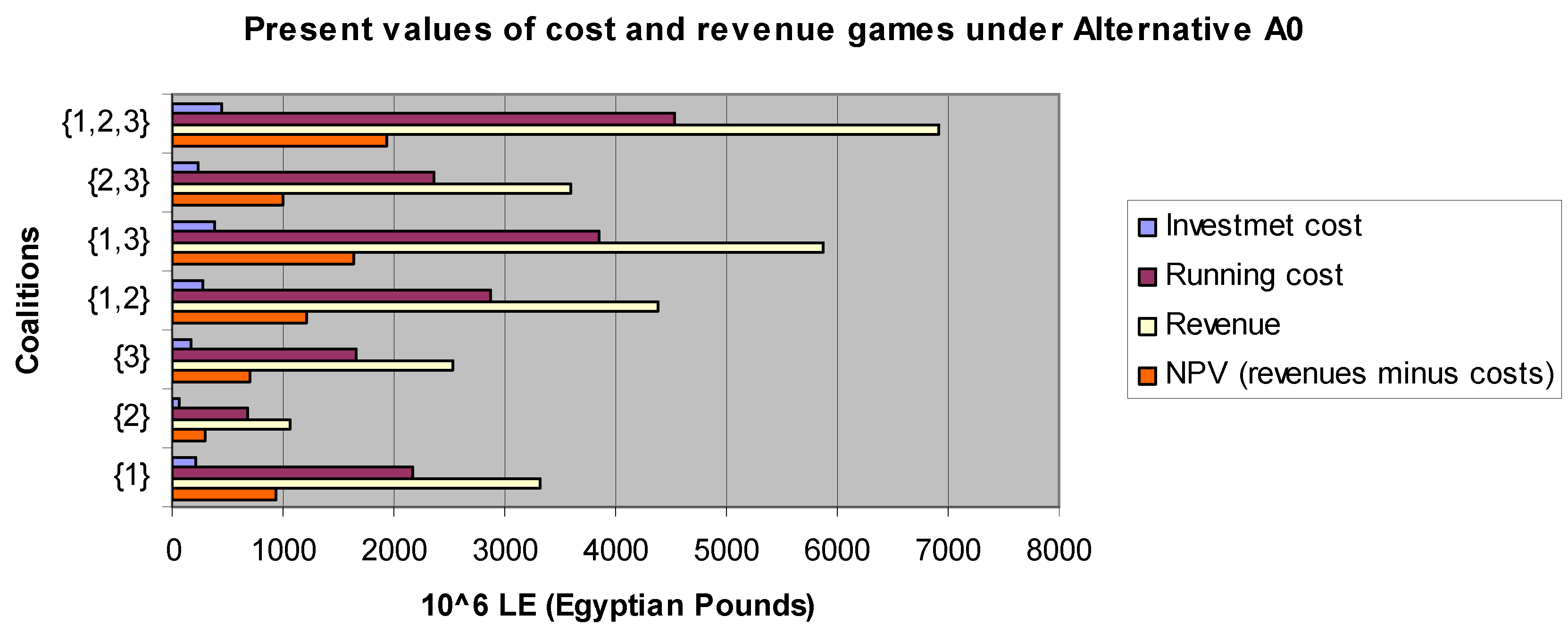
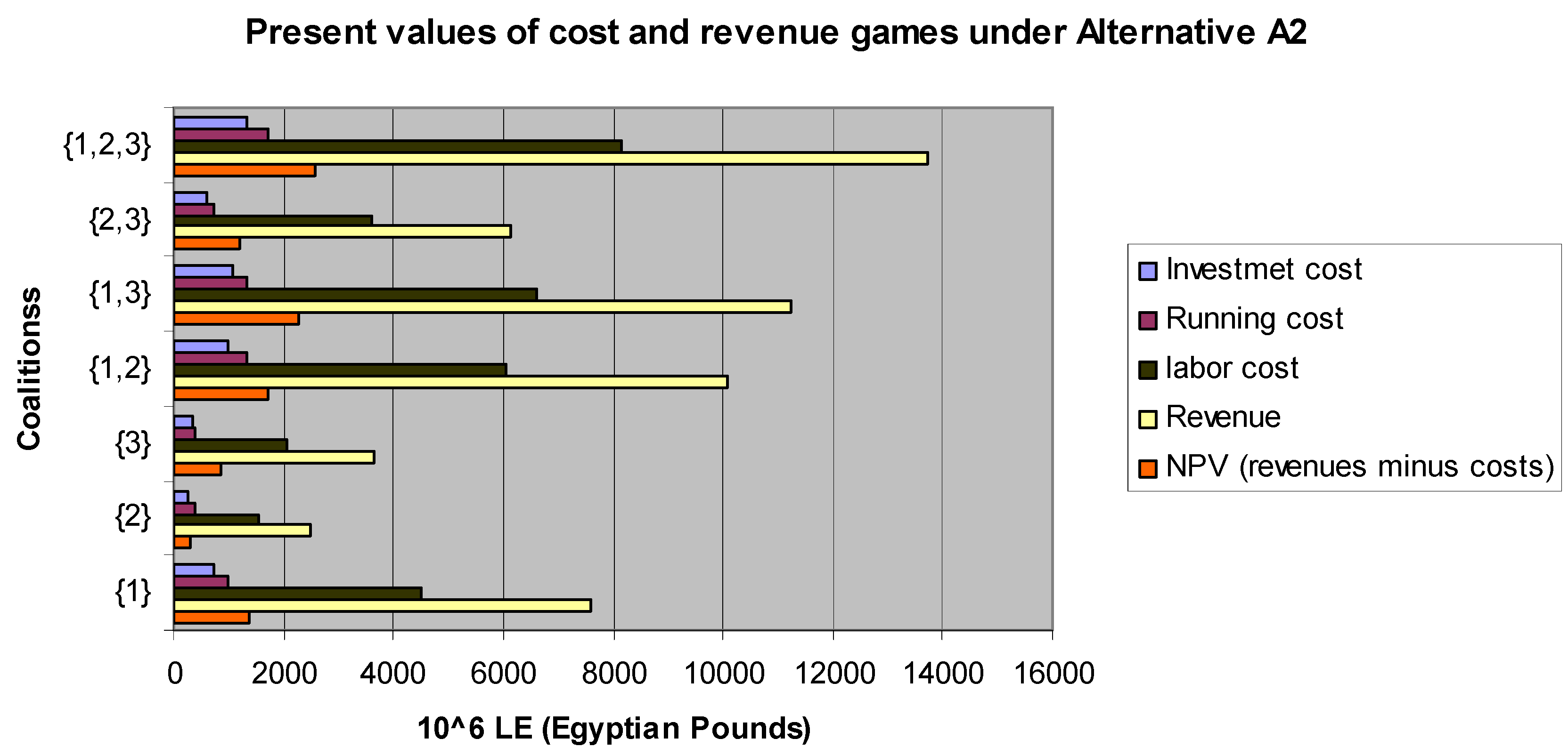
The present values of investment and running costs together with the present values of the revenues under the two different alternatives over a period of twenty years are shown in
Table 22 and
Table 23. The present values of the investment costs under alternatives A0 and A2 are denoted by i
A0 and i
A2, respectively. The present value of the running costs for alternative A0 is denoted by a
A0. Under alternative A2, we distinguish between the present value of running cost game r
lp due to labor, denoted by a
lp, and the present value of the sum of running cost games r
A2,1 + r
A2,2 + r
A2,3, denoted by a
A2 (the present values games i
A2 and a
A2 will be also used in the cost sharing problem introduced in the next section). Finally, the present values of the revenue games under the two alternatives A0 and A2 are denoted by V
A0 and V
A2, respectively.
The last rows of
Table 22 and
Table 23 provide the difference between the present values of the revenue game minus the present value of the cost games under the two alternatives A0 and A2, respectively. Note that the NPV of alternative A2 is larger than the one of alternative A0, for each coalition S ⊆ {1,2,3}, suggesting that alternative A2 is more profitable than A0 over the entire period. The data presented in
Table 22 and
Table 23 are synthetically reported in
Figure 3 and
Figure 4, respectively.
From the results in
Table 22 and
Table 23 we can realize that the net present value of alternative A2 is superior to that of alternative A0 for each coalition of land sections in the project. Therefore, the implementation of alternative A2 is the best option for all intermediate coalitions of all regions. This is consistent with the analysis in
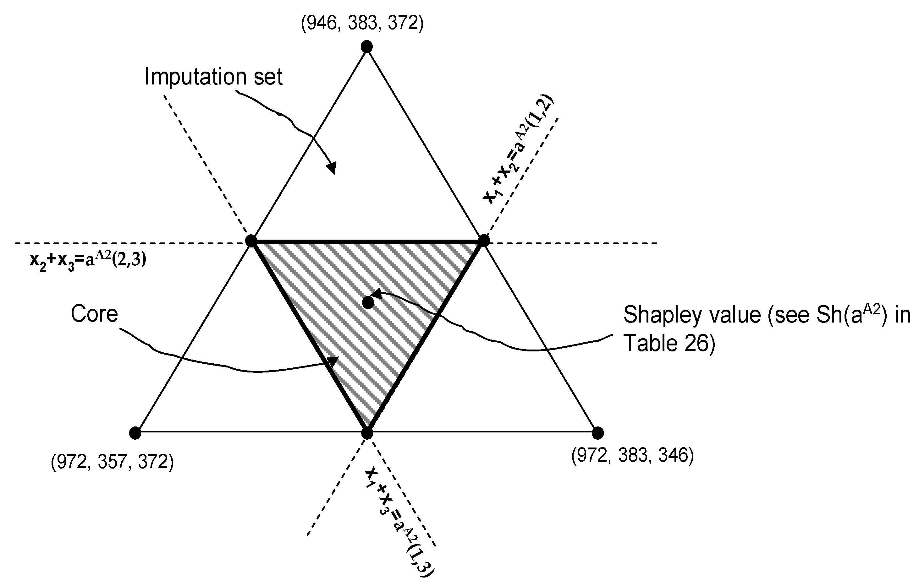
Section 7.1, where the allocation problem of the joint implementation costs for alternative A2 is studied. Of course, such allocation problem must take into account both the effects of time on the cash flow (mainly affecting the actualization of the yearly running costs) and the strength of each coalition S ⊆ {1,2,3} in contributing to the total cost of implementation of alternative A2 in the entire region N. Our next assignment in the paper is to find an allocation of the (investment plus running) cost game in which all the players (land sections) are not unhappy with such an allocation, that is, we will find an allocation which is in the core of the game. We will show that the Shapley Value of the cost game under alternative A2 (for both investment and running costs) is in the core of the cost game (see
Figure 5). Moreover the Shapley value satisfies some nice properties of fairness in general. Thus, we propose the Shapley value of the cost game under alternative A2 as a basis for allocating the costs of implementation of alternative A2 of this game. The Core and the Shapley Value are displayed in
Figure 5.
7.1. Cost Allocation Problem under Alternative A2
We are now ready to suggest ways to allocate the joint costs among the various players (regions). First we summarize which games have been considered, that is, the costs of implementation of alternative A2 that have been adopted for the three regions and analyzed in the previous sections.
Concerning the running costs, in this section we consider the cost allocation problem related to the running cost game a
A2 provided in
Table 23, that is the present value of the sum of the running cost games r
A2,1 + r
A2,2 + r
A2,3. Note that the game r
lp concerning the cost of labor and production is not considered here because, as we previously said, the allocation problem for these costs is clearly defined: each individual farm will support its own cost of labor and production.
Investment costs c
A2 (see
Table 8) are deflated to present time and, as described in [
13], will be probably depreciated over 20 years. Similar to the previous section, for the investment costs, from [
14] we estimated IDC costs at 6.5%, yielding the game î
A2 = 1.065 × c
A2 as shown in
Table 24.
Table 25 summarizes the present value a
A2 of the total running cost for the implementation of alternative A2, as defined in the previous section (
Table 23).
The Shapley values
Sh of the games î
A2(S) and a
A2(S) computed according to relation (1) are shown in
Table 26.
The Shapley allocations in the games Sh(îA2) and Sh(aA2) are in the core of games iA2 and aA2, respectively, and, consequently, the allocations under Sh(îA2 + aA2) is in the core of game iA2 + aA2.
Normalizing all data with respect to the cost allocated by the Shapley value to one single Feddan in the central region, the remaining regions should pay proportionally to the values presented in the
Table 27.
Note that, if the Shapley value is implemented as an allocation method, then because the investment cost game is almost additive, the fraction of investment costs allocated to one Feddan on the project area is the same for all regions. In other words, the Shapley value assigns to one Feddan in the Northern region a smaller fraction of the running costs than in the Southern region and an intermediate fraction in the Central one.
Finally, based on the previous analysis we propose a tariff based on the Shapley value of the cost game that was considered in this paper. We assume a loan for the entire cost of investments (with annual fixed interest rate equal to 4.5%).
Table 28 reports our proposed tariff based on the Shapley Value allocations. The tariff is composed of a fixed amount (per Feddan) plus a per m
3 cost.
8. Conclusions and Epilogue
The Government of Egypt and several financing institutions, led by the World Bank designed the West Delta Water Conservation and Irrigation Rehabilitation Project. The project was motivated by the loss in agricultural land productivity and deteriorated groundwater quality that jeopardized the promising development of the region of the West Delta in Egypt. The project was based on several premises, including a maximum surface water delivery of 5000 m3 per year per Feddan; a conjunctive use of surface and groundwater resources; a full cost recovery of all investment and operation and maintenance costs; and management of the project by the private sector with only government guarantees to reduce risk faced by the private operator. An independent regulator will monitor and enforce the terms of contracts between the beneficiaries and the service provider.
The project documents [
15] propose a single two-part tariff to be charged to all users. The fixed part of the tariff (1272 LE/Feddan per year) was intended to cover capital cost, concession fees, and operator profit. The volumetric part of the tariff (0.15 LE/m
3) was designed to cover the operating costs. These tariffs differ from the once we calculated in our Shapley Value
8.
The Shapley Value tariff per volumetric unit of water is designed such that it takes into consideration the heterogeneous conditions in the different land sections of the project site, which are reflected in differential volumetric fees computed for each section, based in this paper, on height to water table of the aquifer
9. The Shapley Value fixed tariff of 849 (LE/Feddan/year) for all sections is the result of the investment data we had, which was available for the entire land area of the project.
After tireless attempts to recruit private sector bidders to the project with no success, the project was canceled on 30 June 2011 [
12]. Reasons for no interest in the project on the part of the private sector bidders were: (1) high financial risks; (2) proposed government guarantees were not sufficient for private sector entrepreneurs under existing institutions in the country; and (3) collection of the irrigation tariff seemed subject to high transaction costs. From the government point of view, the reasons were: (1) lack of private sector interest in the project; and (2) unrealistically high tariff in the only submitted bid [
12]. Given the dire need of farmers’ for new water supply and their continued request for a solution, the idea of the project will remain alive. It takes more proactive role from all parties if the private sector involvement will be an option.
Based on the above, one could look at our paper as an unsuccessful academic effort. However, the fact that the proposed Shapley-based differential tariff could be by itself an improved version of the single tariff, taking into account the physical characteristics of the main land sections of the project, and the fact that the proposed Shapley-based differential tariff was efficient (recovering all costs) is by itself a reason for making it more attractive to the users and thus reducing the no-payment risk faced by the service provider. Our paper demonstrated the use of cooperative game theory approach in real life decision associated with development and sustainability of scarce water resources. We guided the interested reader through the process we developed to calculate the needed parameters in the cost allocation scheme we proposed. If indeed the Government of Egypt and the World Bank, or any other international development agency will revive this project, we would suggest to use the results of our Shapley Value to conduct a study that will estimate the willingness to pay based on the Shapley Value and on a comparative one tariff to represent alternative A2. Having these responses from the project beneficiaries could shed light on the stability and sustainability of projects that rely on cost allocation of the joint cost.


