Article

Evolutionary Game between Commensal and Pathogenic Microbes in Intestinal Microbiota

Material Measurement Laboratory, National Institute of Standards and Technology, 100 Bureau Drive, Gaithersburg, MD 20899, USA
*
Author to whom correspondence should be addressed.
Submission received: 27 April 2016 / Revised: 6 September 2016 / Accepted: 7 September 2016 / Published: 12 September 2016
(This article belongs to the Special Issue Real World Applications of Game Theory)

Abstract

:
The human intestinal microbiota plays a fundamental role in host health and is associated with many diseases when the homeostasis is disturbed. Although recent achievements in metagenomic sequencing have begun to reveal the variety of microbial composition associated with healthy and disease states, species-specific interactions and systematic dynamics still pose a great challenge to resolve the complexity of human microbiota. Using Clostridium difficile infection in human intestinal microbiota as an example, we apply evolutionary game theory to gain a fundamental understanding of the phenotypic variability and dynamic progression of microbiota. Here, microbiota dynamics are determined by the frequency-dependent fitness of each phenotypic population in the presence of the others. More specifically, the fitness is a function of phenotypic composition of the microbiota. We show how the phenotypic variability of microbiota can be explained by game theoretical approach. Knowledge of this study provides a new perspective in administrating antibiotic when dealing with pathogenic invasion. Instead of solely targeting to pathogens, therapies should aim at the whole ecosystem by reducing the fitness of pathogens compared to that of commensal microbes. In this case, the system will eradicate the pathogens by itself.

1. Introduction

The human intestinal microbiota contains at least 1011 bacteria per gram of intestinal content [1] (p. 9), which play a key role in development and maintenance of systematic homeostasis. The mutually beneficial relationship between the host and microbiota is constantly modulated by the production of metabolites by microbes and these complex and dynamic interactions greatly influence the host’s susceptibility to disease [2] (p. 9). Based on metagenomics measurements, over 80% of human intestinal bacteria fall into two phyla: Firmicutes (37% to 48%) and Bacteroidetes (49% to 56%) [3] (p. 9). The composition of microbiota is complex because (1) each phylum includes thousands of strains of bacteria, and (2) even among healthy people, different diet habits and other factors result in significantly different composition of microbiota [4] (p. 9). Previous work based on principal component analysis of metagenomics data has shown that two principle components, one represents antibiotic-sensitive phenotype and the other represents antibiotic-tolerant phenotype, can account for 70% of variations [3] (p. 9) of intestinal microbiota during antibiotic treatment. Therefore, in a previous model, composition of the symbiotic microbiota has been simplified to antibiotic-sensitive and antibiotic-tolerant bacteria [5] (p. 9).
When the intestinal microbial community loses its homeostasis due to perturbation, a state of dysbiosis can emerge and that is associated with a number of diseases such as obesity, diabetes and inflammatory bowel diseases [6] (p. 9). One of the intestinal dysbiotic diseases induced by a single strain of bacteria is Clostridium difficile (recently reclassified to Peptoclostridium difficile [7] (p. 9)) infection, which causes nearly half a million cases of diarrhea and colitis, resulting in approximately 14 thousands of deaths in the United States per year [8] (p. 9). C. difficile are resistant to fluoroquinolone antibiotics such as ciprofloxacin and levofloxacin. It is widely believed that antibiotic treatment can deplete intestinal commensal bacteria and provides C. difficile with a growth advantage, after which C. difficile can release its toxins to inhibit susceptible microbiota [9] (p. 9). Unfortunately, even though antibiotic treatment using metronidazole or vancomycin is initially effective at treating C. difficile infections, relapse often occurs within 3 months. Over 80% of such recurrent C. difficile infections can be cured using a novel probiotic therapy called fecal microbiota transplantation (FMT) [10,11] (p. 9). Which shifts the microbiota composition of the recipient toward that of the donor [12] (p. 9). The effectiveness of such probiotic therapy also indicates the importance of intestinal microbial composition on the maintenance of human health.
Another essential characteristic of microbiota is the interactions among various types of community microbes. Such interactions determine future changes of microbial composition. From a biomolecular point of view, interspecies exchange of metabolites should play an important role in the evolution and dynamics of intestinal microbial communities [13] (p. 9). This results in species-specific commensal, parasitic, mutualistic, or competitive interactions [14] (p. 9). Commensal bacteria constantly compete with pathogenic bacteria for attachment sites on the surface of intestinal epithelial cells and nutrients for optimal proliferation; they can even directly inhibit each other by secreting antimicrobial compounds [15] (p. 9). Given this complexity, a theoretical framework summarizes individual behavior into the community-level is needed.
Numerous ecological models have been used to study the complex dynamics of the human microbial systems [16,17] (p. 9). Here we choose evolutionary game theory [18,19] (p. 9) to explore an intriguing nature of human microbiota: the growth rate of each member of the microbial community is often influenced by the abundance of other members of the community. To address a real world application of game theory, we demonstrate how prior biomedical knowledge helps us in defining the game of microbiota. Focusing on a model of C. difficile infection, we discuss various scenarios that depend on the nonlinear interactions among three bacterial phenotypes to predict dysbiotic progression and the emergence of disease state.

2. Methods: Model Description

Here we propose a minimal model to capture the dynamics of the human gut microbiota challenged with C. difficile infection. As with previously described models the commensal microbiota has been simplified into two phenotypic groups: antibiotic-sensitive bacteria (denoted as CS) and antibiotic-tolerant bacteria (denoted as CT) [5] (p. 9). In addition, we consider a third phenotypic group of pathogenic bacteria (denoted as PA) to represent the possible presence of C. difficile. The PA bacteria are normally kept in low numbers unless the balance of intestinal microbiota is perturbed. In each scenario, we assume that the model parameters are constants in time and that the populations are well-mixed.
Based on the evolutionary game theory, the presence of each phenotypic group affects each group’s growth rate. In other words, the fitness (growth rate) of each phenotype depends on the frequency of each phenotype, with the coefficient also known as the payoff. In this 3-player game, the payoffs can be denoted as a 3 by 3 matrix describing the effect of pairwise interactions on each phenotype’s growth rate. The payoff is in unit of fitness (relative production rate).
We denote by xi (t) the frequencies of each phenotype: x1 (t) (CS cells), x2 (t) (CT cells) and x3 (t) (PA cells), with x1 (t) + x2 (t) + x3 (t) = 1. If we assume a linear relationship between the growth rate of each phenotype and the frequencies, the equations describing the time variation of the frequencies become:
x ˙ i = x i ( t ) [ F i ( x 1 , x 2 , x 3 ) F ]
where the fitness (growth rate) of each cell type is determined by a game payoff matrix Aik by
F i ( x 1 , x 2 , x 3 ) = k = 1 3 A i k x k
and the average fitness of the population is:
F = i = 1 3 k = 1 3 x i A i k x k
The payoff matrix Aik is shown in Table 1:
Where the diagonal elements of the payoff matrix are zero because we assume that each phenotype has neutral effect on its own growth rate.
Based on previous work discussed above, and to simplify the set of possible 3-player games to those that capture the essential dynamics of interest here, we consider games with the following rules and assumptions:
  • Over 40% of intestinal microbes cannot be grown in isolated laboratory cultures because it is very difficult to provide all of the appropriate bacteria-secreted growth factors for the complex intestinal microbiota community. Therefore, we assume CS and CT bacteria depend on each other for optimal proliferation, resulting in positive values for “a” and “c” in the payoff matrix. The resulting 2-player game, with just CS and CT phenotypes, is similar to a Snowdrift game. In a Snowdrift game, individuals gain direct benefits from cooperative acts, resulting in an evolutionary stable strategy state (coexistence). This is consistent with the observation that if the fraction of PA cells is negligible, there is a stable coexistence between CS and CT cells [5] (p. 9).
  • Regarding the pairwise interaction between CS and PA: without antibiotics administration, CS population usually inhibits PA population. However, PA population takes over CS population when antibiotics were administrated. The resulting 2-player game is very similar to a Prisoner’s Dilemma, in which the two strategies (or players) do not stably coexist. In other words, only one evolutionary stable strategy can exist. Therefore, we assume one player gains while the other loses, represented by the payoffs of CS vs. PA (“e”) and PA vs. CS (“b”) with opposite signs.
  • Likewise, when CS population is suppressed by antibiotics, two scenarios may occur: (1) PA and CT compete for resources so that the payoffs of PA vs. CT (“d”) and CT vs. PA (“f”) are both negative; (2) PA exploits CT for resources so that the payoff of PA vs. CT (“d”) is positive and the payoff of CT vs. PA (“f”) is negative. Therefore, in any case we assume that the CT population declines in the presence of PA cells, with a negative payoff “f.”
We reduce the payoff matrix Aik to the minimal payoff matrix Bik (Table 2) by taking into account that the nature of fixed points of evolutionary dynamics remains unaffected under a projective transformation of the relative population frequencies. By rescaling the relative frequencies (x1, x2, x3), we can change the location of the fixed points on the phase diagram, without changing their stabilities. We can rescale Aik by a factor of (a, c, −f) (note that f is negative) such that β = −b/a = e/(−f) and α = d/c. Then the minimal payoff matrix Bik becomes:
Where α and β can be either positive or negative numbers. The PA population may grow (or decline) in the presence of CT bacteria if the sign of α is positive (or negative). Similarly, the CS bacteria gain (or lose) fitness from PA bacteria depending on whether β is positive (or negative). In the minimal payoff matrix, we assume CS population gains exactly what PA population loses in growth rate (β) when they interact. A biological explanation is that one population may acquire the attachment sites or metabolic resources from the other population, and which population will take over is determined by the existence of antibiotics. However, each column in the minimal payoff matrix can be rescaled to fit experimental or clinical data, which results in relocating the fixed points without loss of the nature of their stability.

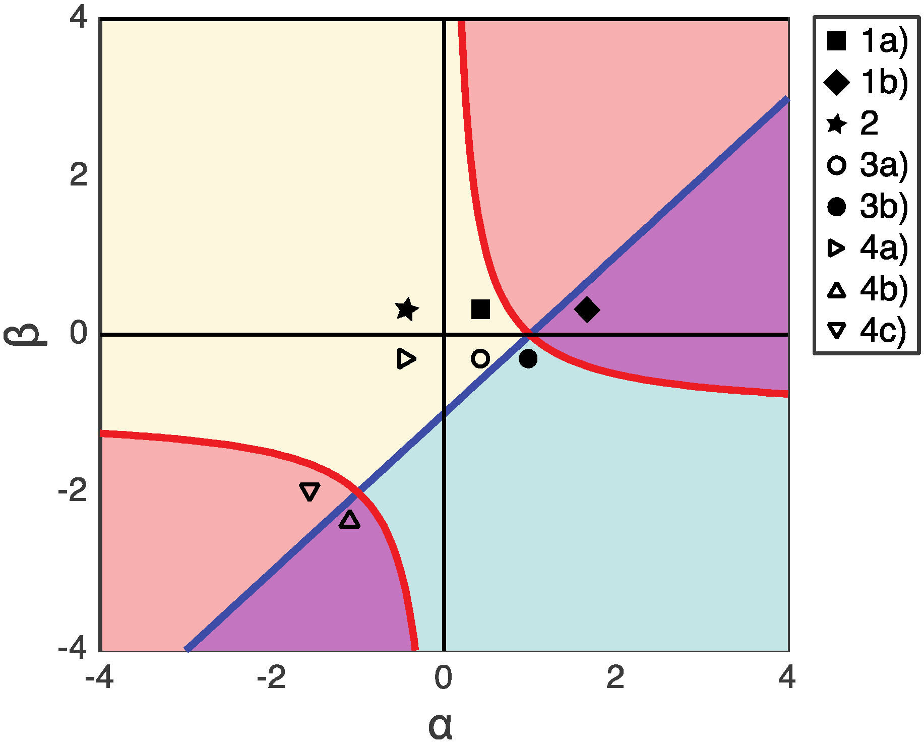
3. Results: Fixed Points and Stability Analysis

In the following sections, we will discuss four models focusing on the effects of CS and CT on PA proliferation depending on the values of α and β. The model that PA bacteria benefit from CT but are suppressed by CS, and the model that CT and CS both suppress PA are presented in Section 3.1. The model that PA bacteria benefit from both CS and CT is presented in Section 3.2. Finally, we present the model that PA population is suppressed by CT but benefited from CS in Section 3.3.

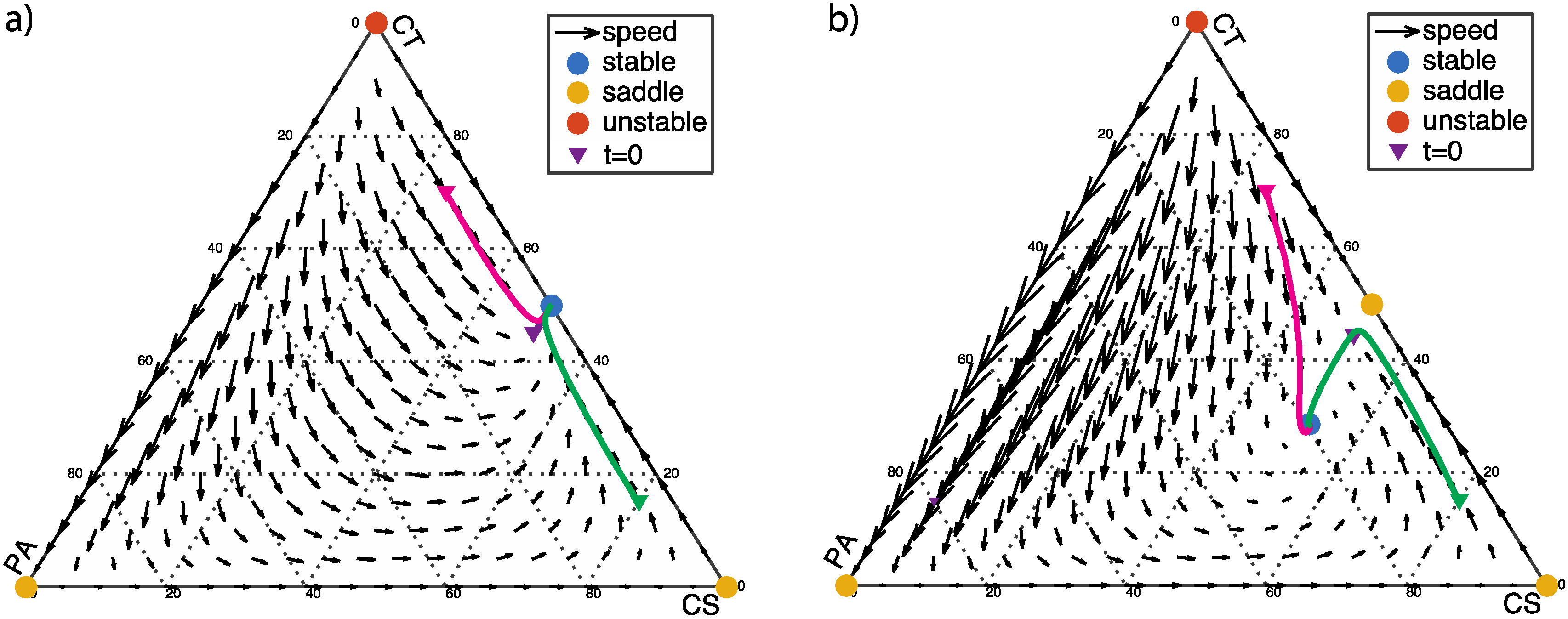
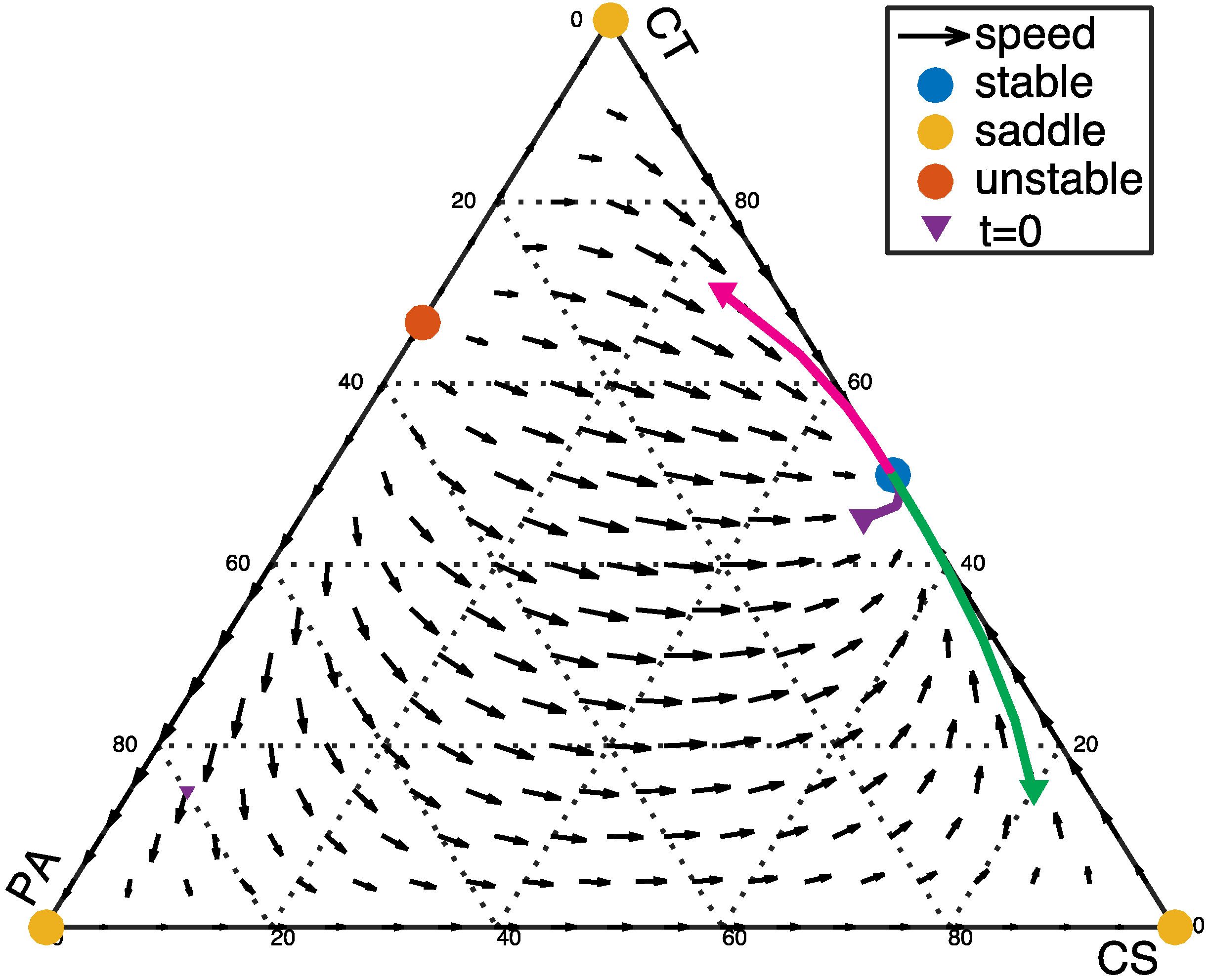
3.1. Single Healthy Stable Fixed Point (β > 0)

We first consider the scenario in which the PA population benefits from the presence of CT bacteria (α > 0) but is inhibited by the presence of CS bacteria (β > 0). This system will have a single stable fixed point, corresponding to a healthy coexistence between CS and CT bacteria with little or no PA bacteria (Figure 1). The fixed points (x *1, x *2, x *3) of the dynamics include two vertices of the simplex (1, 0, 0) and (0, 0, 1) as saddle points, and one vertex (0, 1, 0) as an unstable fixed point. If the PA bacteria benefit only moderately from the CT bacteria (α < β + 1) the stable fixed point will be on the edge of the simplex, at (1/2, 1/2, 0) (Figure 1a). If the PA bacteria benefit more strongly from the CT bacteria (α > β + 1), this point becomes a saddle point (Figure 1b), and the stable fixed point moves to the interior of the simplex at:
( ( α ( β + 1 ) ) 1 ( β + 2 ) ( α + β 1 ) , β ( β + 2 ) ( β + 2 ) ( α + β 1 ) , α β 1 ( β + 2 ) ( α + β 1 ) )
The flow-field diagram of population frequencies as shown in Figure 1 provides an overview of the dynamics of this scenario. In Figure 1, the solid lines indicate the dynamic progression of three different starting populations versus time. The three starting points are chosen to correspond to healthy human controls because pathogenic bacteria such as C. difficile is typically about 5% in clinical samples [20] (p. 9). Near the equilibria, the progression of the dynamics becomes slower. From a clinical perspective, the ideal goal is to eradicate pathogenic bacteria (PA) or at least reach stability with low fraction of PA. Figure 1a shows an ideal condition (α < β + 1), in which PA-free coexistence of CT and CS cells is a stable fixed point. When α > β + 1, the PA, CT, and CS cells coexist at equilibrium, as shown in Figure 1b. This is an acceptable condition clinically since the ratio of three phenotypes reaches a balance regardless to initial population fractions.
On the other hand, the CT and CS bacteria might both suppress the growth of the PA bacteria by producing toxins or through competition for attachment sites and nutrients. In this case, both the CT bacteria and the CS bacteria inhibit the growth of the PA population (α < 0 and β > 0). Again, the system will have only one stable fixed point, on the edge of the simplex at (1/2, 1/2, 0), corresponding to a healthy state with no PA bacteria present. The dynamic progression with various initial population fractions is shown in Figure 2. Regardless of the initial population fractions, the system returns to a healthy state with CS and CT dominating the community.

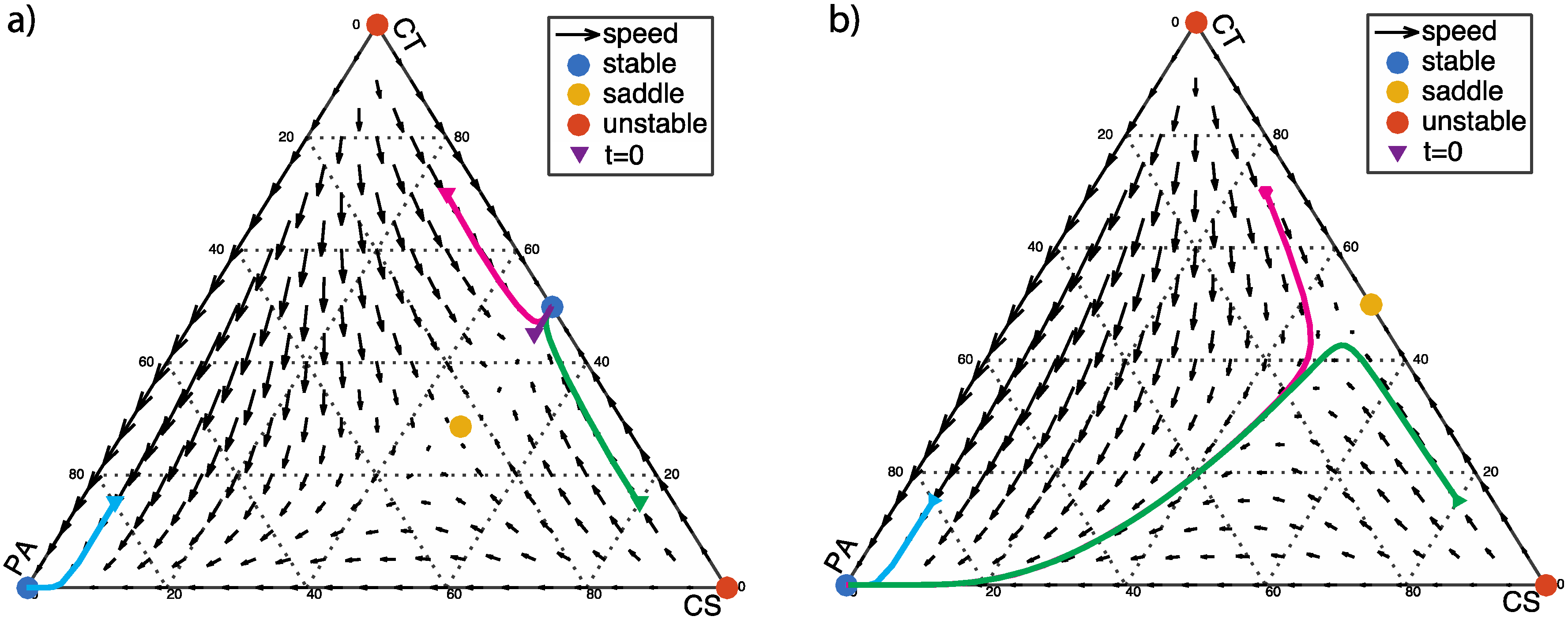
3.2. From Healthy to Dysbiotic States (α > 0 and β < 0)

Here we consider the scenarios in which the PA population benefits from the presence of CT bacteria (α > 0) and from the presence of CS bacteria (β < 0). This would be the case, for example, if the PA bacteria require metabolites produced by both the CT and CS populations for optimal growth. In this case, the pure pathogenic vertex at (0, 0, 1) is a stable fixed point, and a persistent dysbiosis (PA dominance) can occur.
If the PA bacteria benefit only moderately from the CT bacteria (α < β + 1), there is an additional stable fixed point at (1/2, 1/2, 0), as shown in Figure 3a. This indicates that the system can tolerate a certain level of PA infection. If PA fraction is low, eventually PA bacteria will be extinguished in favor of a stable community consisting only of CS and CT. If the PA fraction is too high, however, PA bacteria will eventually dominate the community. If the PA bacteria benefit strongly from the CT bacteria (α > β + 1), the vertex at (0, 0, 1), representing a dysbiotic state, is the only stable fixed point; and the point at (1/2, 1/2, 0) is a saddle point (Figure 3b). PA will eventually dominate the community, regardless of the initial population fraction.
The dynamic progressions for different starting populations are shown as the solid lines in Figure 3. In addition to the starting points corresponding to healthy states, an additional starting point with population fractions of CS, CT, and PA cells (x10, x20, x30) = (0.05, 0.15, 0.8) is labeled with light blue in Figure 3. This starting point is chosen as an extreme case when C. difficile fraction exceeds 70%, which has been shown to occur under the misusage of metronidazole or lacticin antibiotics [20] (p. 9).

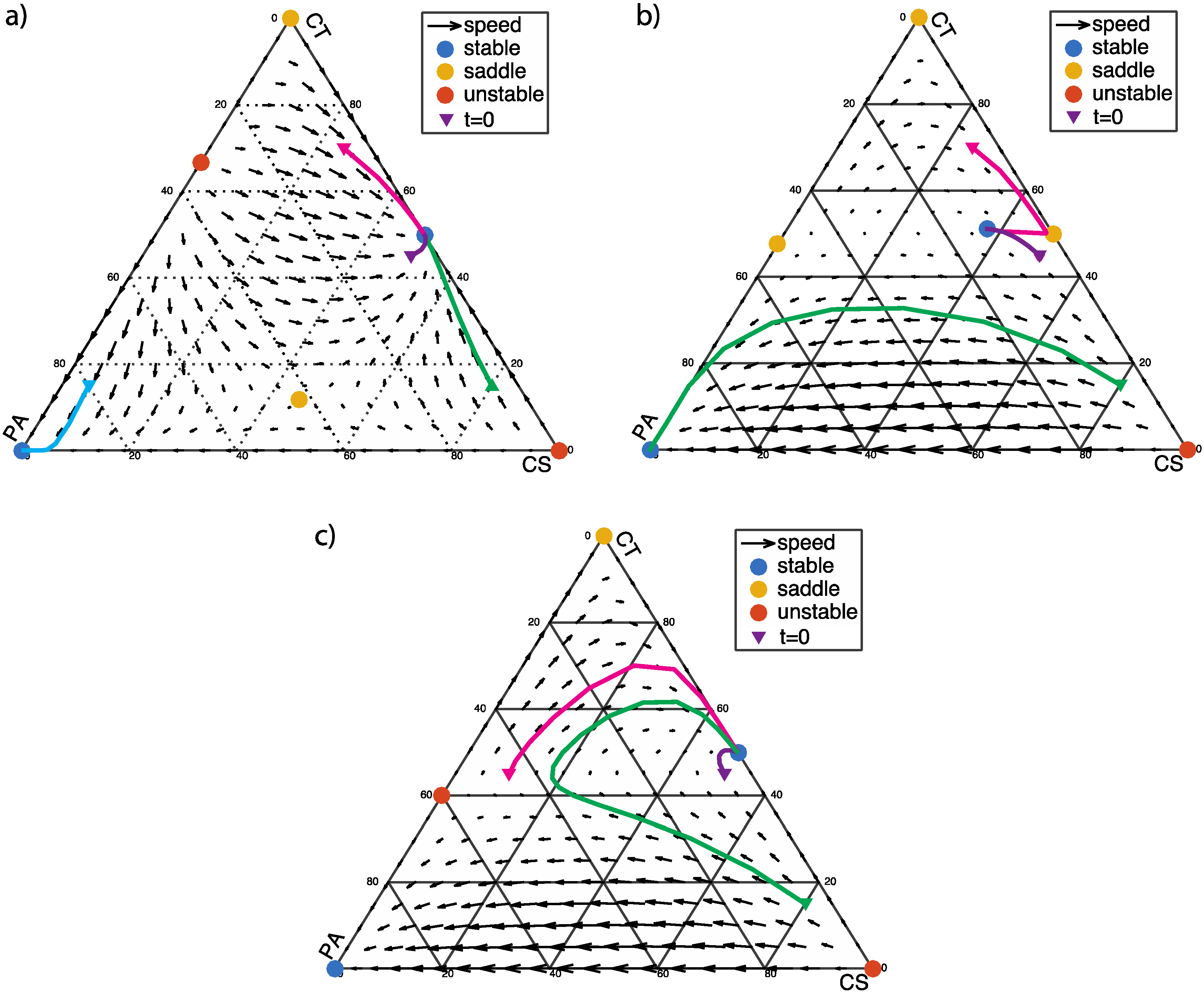
3.3. Two Stable Fixed Points: Healthy and Dysbiotic (α < 0 and β < 0)

Now we discuss the scenario in which the PA population is inhibited by the presence of CT bacteria (α < 0) but benefits from the presence of CS bacteria (β < 0). In this scenario, there are always two stable fixed points: the vertex at (0, 0, 1), representing the dysbiotic state; and a second stable fixed point on or near the edge of the simplex, representing a healthy coexistence of CT and CS bacteria with little or no PA bacteria (Figure 4).
If the three phenotypic groups are weakly interacting (α < β + 1 and α (β + 1) < 1), the healthy stable point is on the edge of the simplex at (1/2, 1/2, 0) (Figure 4a). The dynamic behavior is similar to Figure 3a, which may tolerate certain level of PA infection. Low level of PA will be extinguished regardless the fractions of CS or CT. High level of PA will take over the microbial community. The difference is that, in this case there is an unstable fixed point at the edge (PA-CT) so that the tolerance of PA infection is higher than the case in Figure 3a.
If CT bacteria moderately inhibit PA bacteria (α > β + 1 and α (β + 1) > 1), the stable fixed point moves to the interior of the simplex (Figure 4b). With the PA frequency starting at a low level (0.05), which stable fixed point the system flows to will depend on the CT frequency. If the CT frequency is high enough (>0.4), the system flows toward the healthy state with coexistence of the three phenotypes. Otherwise, the system flows toward the dysbiotic state and PA will eventually dominating the population.
If CT bacteria strongly inhibit PA bacteria (α < β + 1 and α (β + 1) > 1), the healthy stable point is on the edge of the simplex at (1/2, 1/2, 0), as shown in Figure 4c. The system exhibits a certain level of tolerance to PA infection. With a starting PA frequency of 0.05, as long as CT level is above 0.15, the PA cells will be extinguished. Otherwise, PA cells will dominate the whole population.

4. Discussion

We have discussed various scenarios based on the relative gain or loss of fitness of the PA phenotype represented by the values of α and β. In Figure 5, we summarize the results, indicating regions of the α vs. β phase diagram with a single stable fixed point (solid markers), and those with bistability (open markers) in the dynamical system. The question of whether there is one or two stable fixed points is important because that will determine how much perturbation of microbial composition can be tolerated by the host system. The parameters α and β together with population composition determine if the system is able to recover from an abrupt dysbiotic state caused by pathogenic invasions or antibiotic disturbance [21] (p. 9).
If fluoroquinolone antibiotics were administrated, the balance of microbial system would be perturbed. Pathogens such as C. difficile are usually inhibited by commensal bacteria (especially CS) until fluoroquinolone antibiotics gradually eradicate most antibiotic-sensitive CS bacteria. When CS is weakened (β < 0), two possible scenarios may occur: (1) PA strongly exploits CT (α > β + 1 > 0), then C. difficile infection will arise; (2) CT competes with PA (α < 0). If CT sufficiently inhibits PA in the competition among CT and PA bacteria, then C. difficile infection may not occur. Therefore, the outcome of the competition can be determined by the value of α.
Although the model concerns a well-mixed population without spatial structure, it still provides some potential therapeutic insights. The stable fixed point is the state of least energy that the system will inhabit for an indefinite length of time. When the system has only one stable fixed point, there is a unique “absolutely stable’’ state that the system will return to after perturbations. When the system has two stable fixed points, it is important to consider whether the dysbiotic fixed point is globally stable or merely metastable, and what clinical interventions will shift the system to a state that will flow toward the desired healthy fixed point. Such nonlinear characteristics are usually neglected in clinical practice, which in general follows the strategy of “immediately administrate antibiotics when pathogen infection is observed.” Better understanding of the population dynamics could help reduce the overuse of antibiotics and the resulting emergence of antibiotic resistance [22] (p. 10). In the highly simplified scenario described by our model, if we could effectively tune the system parameters α and β by readjusting host biochemical environment, or the population composition by taking probiotics, the system could be made to eradicate PA cells with the help of CS and CT cells.
The validation of theoretical models for microbial community dynamics will require measurements of mixed population composition with high temporal resolution. Recent top-down approaches in molecular “omics’’ such as 16s RNA sequencing provide abundant information about the composition of microbial cells in nature [23] (p. 10). However, there are few time-course metagenomic analyses, which require a lot of resources but can be helpful in unraveling the microbial community dynamics [24] (p. 10). A bottom-up synthetic approach would be to mix additional types of microbes one at a time, creating tightly controlled experimental model systems [14] (p. 9). Such model systems can exhibit complex community interactions such as cooperative digestion or by-product exchange, but are tractably limited to a small number of strains that can be cultured in the lab. We hope this study would inspire more experimental and modeling works which may help bridge the gap between top-down systems approach and bottom-up synthetic approach toward an understanding of complex microbial systems.

Acknowledgments

A.W. is supported by the National Institute of Standards and Technology/National Research Council Postdoctoral Fellowship Program. We thank J. Kralj for discussions.

Author Contributions

All authors designed and conducted the research and wrote the manuscript.

Conflicts of Interest

The authors declare no conflict of interest.

References

  1. Tlaskalová-Hogenová, H.; Stěpánková, R.; Kozáková, H.; Hudcovic, T.; Vannucci, L.; Tučková, L.; Rossmann, P.; Hrnčíř, T.; Kverka, M.; Zákostelská, Z.; et al. The role of gut microbiota (commensal bacteria) and the mucosal barrier in the pathogenesis of inflammatory and autoimmune diseases and cancer: Contribution of germ-free and gnotobiotic animal models of human diseases. Cell. Mol. Immunol. 2011, 8, 110–120. [Google Scholar] [CrossRef] [PubMed]
  2. Nicholson, J.K.; Holmes, E.; Kinross, J.; Burcelin, R.; Gibson, G.; Jia, W.; Pettersson, S. Host-gut microbiota metabolic interactions. Science 2012, 336, 1262–1267. [Google Scholar] [CrossRef] [PubMed]
  3. Dethlefsen, L.; Relman, D.A. Incomplete recovery and individualized responses of the human distal gut microbiota to repeated antibiotic perturbation. Proc. Natl. Acad. Sci. USA 2011, 108, 4554–4561. [Google Scholar] [CrossRef] [PubMed]
  4. Wu, G.D.; Chen, J.; Hoffmann, C.; Bittinger, K.; Chen, Y.Y.; Keilbaugh, S.A.; Bewtra, M.; Knights, D.; Walters, W.A.; Knight, R.; et al. Linking long-term dietary patterns with gut microbial enterotypes. Science 2011, 334, 105–108. [Google Scholar] [CrossRef] [PubMed]
  5. Bucci, V.; Bradde, S.; Biroli, G.; Xavier, J.B. Social interaction, noise and antibiotic-mediated switches in the intestinal microbiota. PLoS Comput. Biol. 2012, 8, e1002497. [Google Scholar] [CrossRef] [PubMed]
  6. Carding, S.; Verbeke, K.; Vipond, D.T.; Corfe, B.M.; Owen, L.J. Dysbiosis of the gut microbiota in disease. Microb. Ecol. Health Dis. 2015, 26. [Google Scholar] [CrossRef] [PubMed]
  7. Yutin, N.; Galperin, M.Y. A genomic update on clostridial phylogeny: Gram-negative spore formers and other misplaced clostridia: Genomics update. Environ. Microbiol. 2013, 15, 2631–2641. [Google Scholar] [CrossRef] [PubMed]
  8. Ananthakrishnan, A.N. Clostridium difficile infection: Epidemiology, risk factors and management. Nat. Rev. Gastroenterol. Hepatol. 2011, 8, 17–26. [Google Scholar] [CrossRef] [PubMed]
  9. Antharam, V.C.; Li, E.C.; Ishmael, A.; Sharma, A.; Mai, V.; Rand, K.H.; Wang, G.P. Intestinal Dysbiosis and Depletion of Butyrogenic Bacteria in Clostridium difficile Infection and Nosocomial Diarrhea. J. Clin. Microbiol. 2013, 51, 2884–2892. [Google Scholar] [CrossRef] [PubMed]
  10. Bakken, J.S. Fecal bacteriotherapy for recurrent Clostridium difficile infection. Anaerobe 2009, 15, 285–289. [Google Scholar] [CrossRef] [PubMed]
  11. Brandt, L.J.; Aroniadis, O.C.; Mellow, M.; Kanatzar, A.; Kelly, C.; Park, T.; Stollman, N.; Rohlke, F.; Surawicz, C. Long-term follow-up of colonoscopic fecal microbiota transplant for recurrent Clostridium difficile infection. Am. J. Gastroenterol. 2012, 107, 1079–1087. [Google Scholar] [CrossRef] [PubMed]
  12. Khoruts, A.; Dicksved, J.; Jansson, J.K.; Sadowsky, M.J. Changes in the composition of the human fecal microbiome after bacteriotherapy for recurrent Clostridium difficile-associated diarrhea. J. Clin. Gastroenterol. 2010, 44, 354–360. [Google Scholar] [CrossRef] [PubMed]
  13. Harcombe, W.; Riehl, W.; Dukovski, I.; Granger, B.; Betts, A.; Lang, A.; Bonilla, G.; Kar, A.; Leiby, N.; Mehta, P.; et al. Metabolic Resource Allocation in Individual Microbes Determines Ecosystem Interactions and Spatial Dynamics. Cell Rep. 2014, 7, 1104–1115. [Google Scholar] [CrossRef] [PubMed]
  14. Wintermute, E.H.; Silver, P.A. Dynamics in the mixed microbial concourse. Genes Dev. 2010, 24, 2603–2614. [Google Scholar] [CrossRef] [PubMed]
  15. Payne, A.N.; Zihler, A.; Chassard, C.; Lacroix, C. Advances and perspectives in in vitro human gut fermentation modeling. Trends Biotechnol. 2012, 30, 17–25. [Google Scholar] [CrossRef] [PubMed]
  16. Costello, E.K.; Stagaman, K.; Dethlefsen, L.; Bohannan, B.J.M.; Relman, D.A. The application of ecological theory toward an understanding of the human Microbiome. Science 2012, 336, 1255–1262. [Google Scholar] [CrossRef] [PubMed]
  17. Zomorrodi, A.R.; Segrè, D. Synthetic Ecology of Microbes: Mathematical Models and Applications. J. Mol. Biol. 2015, 428, 837–861. [Google Scholar] [CrossRef] [PubMed]
  18. Maynard Smith, J. Evolution and the Theory of Games; Cambridge University Press: Cambridge, New York, NY, USA, 1982. [Google Scholar]
  19. Hofbauer, J.; Sigmund, K. Evolutionary Games and Population Dynamics; Cambridge University Press: Cambridge, New York, NY, USA, 1998. [Google Scholar]
  20. Rea, M.C.; Dobson, A.; O’Sullivan, O.; Crispie, F.; Fouhy, F.; Cotter, P.D.; Shanahan, F.; Kiely, B.; Hill, C.; Ross, R.P. Effect of broad- and narrow-spectrum antimicrobials on Clostridium difficile and microbial diversity in a model of the distal colon. Proc. Natl. Acad. Sci. USA 2011, 108, 4639–4644. [Google Scholar] [CrossRef] [PubMed]
  21. Hu, B.; Du, J.; Zou, R.Y.; Yuan, Y.J. An Environment-Sensitive Synthetic Microbial Ecosystem. PLoS ONE 2010, 5, e10619. [Google Scholar] [CrossRef] [PubMed]
  22. Kohanski, M.A.; DePristo, M.A.; Collins, J.J. Sublethal Antibiotic Treatment Leads to Multidrug Resistance via Radical-Induced Mutagenesis. Mol. Cell 2010, 37, 311–320. [Google Scholar] [CrossRef] [PubMed]
  23. Biteen, J.S.; Blainey, P.C.; Cardon, Z.G.; Chun, M.; Church, G.M.; Dorrestein, P.C.; Fraser, S.E.; Gilbert, J.A.; Jansson, J.K.; Knight, R.; et al. Tools for the Microbiome: Nano and Beyond. ACS Nano 2016, 10, 6–37. [Google Scholar] [CrossRef] [PubMed]
  24. Faust, K.; Lahti, L.; Gonze, D.; de Vos, W.M.; Raes, J. Metagenomics meets time series analysis: Unraveling microbial community dynamics. Curr. Opin. Microbiol. 2015, 25, 56–66. [Google Scholar] [CrossRef] [PubMed]
Figure 1. α > 0 and β > 0: (a) α < β + 1, α = 0.5, β = 0.2; (b) α > β + 1, α = 1.5, β = 0.2. The initial population fractions of commensal antibiotic-sensitive bacteria (CS), commensal antibiotic-tolerant bacteria (CT), and pathogenic (PA) cells (x10, x20, x30) = (0.5, 0.545, 0.05), (0.25, 0.7, 0.05), and (0.8, 0.15, 0.05) are labeled with triangle markers.
Games 07 00026 g001
Figure 2. α < 0 and β > 0: α = −0.5, β = 0.2. In this case, the interior fixed point does not exist because the coordinates based on Equation (4) are outside the allowed range of the simplex (0 < xi < 1). The three vertices of the simplex at (1, 0, 0), (0, 1, 0), and (0, 0, 1) are saddle points. In addition, an unstable fixed point with the coordinates (0, 1/(1 − α), −α/(1 − α)) emerges.
Games 07 00026 g002
Figure 3. α > 0 and β < 0: The two vertices of the simplex with pure commensal populations (CS and CT) at (1, 0, 0) and (0, 1, 0) are unstable fixed points. (a) α < β + 1, α = 0.5, β = −0.2; a saddle point with the coordinates given by Equation 4 emerges in the interior of the simplex; (b) α > β + 1, α = 1, β = −0.2.
Games 07 00026 g003
Figure 4. α < 0 and β < 0: The two vertices of the simplex at (1, 0, 0) and (0, 1, 0) are unstable and saddle points, respectively. There are two fixed points at the edges of the simplex: (1/2, 1/2, 0) (coexistence of CS and CT cells) and (0, 1/(1 − α), −α/(1 − α)) (coexistence of CT and PA cells). (a) α < β + 1 and α (β + 1) < 1, α = −0.5, β = −0.2; (0, 1/(1 − α), −α/(1−α)) is an unstable fixed point, and the interior fixed point is a saddle point; (b) α > β + 1and α (β + 1) > 1, α = −1.1, β = −2.2; the points at (1/2, 1/2, 0) and (0, 1/(1 − α), −α/(1 − α)) are saddle points; (c) α < β + 1 and α (β + 1) > 1, α = −1.5, β = −2; (0, 1/(1 − α), −α/(1 − α)) is an unstable fixed point.
Games 07 00026 g004
Figure 5. The payoffs in each figure are shown in α vs. β plane. The regions where α (β + 1) > 1 is shaded with pink color, and the regions where α > β + 1 is shaded with blue color. The overlapped region (α (β + 1)>1 and α > β + 1) is purple. The scenarios with bistability are labeled with open markers. The scenarios with unique stability are labeled with solid markers.
Games 07 00026 g005
Table 1. The payoff matrix.
CSCTPA
CS0ce
CTa0f
PAbd0
Table 2. The minimal payoff matrix.
CSCTPA
CS01β
CT10−1
PA−βα0

