Buying Optimal Payoffs in Bi-Matrix Games

Department of Computer Science, University of Liverpool, Liverpool L69 3BX, UK
*
Author to whom correspondence should be addressed.
Games 2018, 9(3), 40; https://0-doi-org.brum.beds.ac.uk/10.3390/g9030040
Submission received: 23 May 2018
/
Revised: 20 June 2018
/
Accepted: 22 June 2018
/
Published: 26 June 2018
(This article belongs to the Special Issue Logic and Game Theory)
Abstract
:We consider non-zero sum bi-matrix games where one player presumes the role of a leader in the Stackelberg model, while the other player is her follower. We show that the leader can improve her reward if she can incentivise her follower by paying some of her own utility to the follower for assigning a particular strategy profile. Besides assuming that the follower is rational in that he tries to maximise his own payoff, we assume that he is also friendly towards his leader in that he chooses, ex aequo, the strategy suggested by her—at least as long as it does not affect his expected payoff. Assuming this friendliness is, however, disputable: one could also assume that, ex aequo, the follower acts adversarially towards his leader. We discuss these different follower behavioural models and their implications. We argue that the friendliness leads to an obligation for the leader to choose, ex aequo, an assignment that provides the highest follower return, resulting in ‘friendly incentive equilibria’. For the antagonistic assumption, the stability requirements for a strategy profile should be strengthened, comparable to the secure Nash equilibria. In general, no optimal incentive equilibrium for this condition exists, and therefore we introduce -optimal incentive equilibria for this case. We show that the construction of all of these incentive equilibria (and all the related leader equilibria) is tractable.
1. Introduction
Stackelberg models [1] have been studied in detail in Oligopoly Theory [2]. In a Stackelberg model, one player or firm acts as a market leader and the other is a follower. The model is a sequential move game, where the leader takes the first move and the follower moves afterwards. The main objective of both players is to maximise their own return. The Stackelberg model makes some basic assumptions, in particular that the leader knows ex-ante that the follower observes her action and that both players are rational in that they try to maximise their own return. We consider a game setting where one player acts as the leader and assigns a strategy to her follower, which is optimal for herself. This is viewed as a Stackelberg or leadership model, where a leader is able to commit to a strategy profile first before her follower moves. We consider Stackelberg models for non-zero sum bi-matrix games. In our game setting, the row player is the leader and the column player is her follower. In a stable strategy profile, players select their individual strategies in such a way that no player can do better by changing their strategy alone. This requirement is justified in Nash’s setting as the players have equal power. In a leader equilibrium [1], this is no longer the case. As the leader can communicate her move (pure or mixed) up front, it is quite natural to assume that she can also communicate a suggestion for the move of her follower. However, the leader cannot freely assign strategies. Her follower will only follow her suggestion when he is happy with it in the Nash sense of not benefiting from changing his strategy. We refer to strategy profiles with this property as leader strategy profiles. A leader equilibrium is simply a leader strategy profile, which is optimal w.r.t. the leader return.
We argue that a leader with the power to communicate can also communicate her strategy and the response she would like to see from her follower and that—and how much—she is willing to pay for compliance. This allows her to incentivise various strategy choices of her follower by paying him a low bribery value. Incentivising the choice of her follower by paying an incentive would intuitively change the payoff matrices for both players accordingly: it would decrease the leader’s payoff by the amount , and increase the follower’s payoff by the same amount. In this setting, the leader has more power compared to Stackelberg’s traditional setting: the moves there can be viewed as special cases with an incentive of .
Similar to the classic case, the leader is restricted to strategies that the follower is prepared to follow, but, for determining this, the incentive he would gain (when following) or lose (when deviating) is taken into account. We refer to strategy profiles (including the bribery value) that satisfy this constraint as incentive strategy profiles, and to the optimal choices of the leader among them as incentive equilibria. As an example, we refer to a bi-matrix game shown in Table 1.
In this example, the only Nash equilibrium is the strategy profile . This strategy profile is also the leader equilibrium. The leader payoff and the follower payoff in this strategy profile are 0 and 1, respectively. However, if we allow the leader to incentivise her follower for following a particular strategy profile, then she can incentivise her follower to play the pure strategy I by paying him a bribery value of 1. The strategy profile with bribery value 1 is then an incentive equilibrium. The payoffs for the leader and the follower for this equilibrium are 4 and 1, respectively. To see an example where Nash and leader equilibrium in a game are not same, we refer to Table 2. In this example, the strategy profile is the leader equilibrium that is not a Nash equilibrium. It provides a payoff of 2 and 1 to the leader and the follower, respectively. The only Nash equilibrium here is the strategy profile . In the leader equilibrium , the leader has an incentive to deviate to strategy I, but doing so would result in the follower to deviate to strategy I, which would lead to the only Nash equilibrium. This example also shows how the leader benefits from asymmetric strategy profiles in the leader equilibrium.
Like in leader equilibria, the leader can select a strategy profile where she benefits from deviation. We will discuss such a situation based on the example of the Prisoner’s Dilemma [3]. As the entities who interact strategically are often called players, we use the term ’players’ here instead of ’prisoners’. The game has the famous antinomy that both players do better if they both co-operate (C) with each other, while both of them have the dominating strategy to defect (D). Consequently, is the only Nash equilibrium in this game. We recall that a strategy is dominant if it provides maximal payoff to a player, regardless of what the other player would play. It is therefore always better for a player to play a dominant strategy. We refer to the prisoner’s dilemma payoff matrix from Table 3. The only Nash equilibrium here is the strategy profile with a joint return of . Another observation is that leader equilibria are not powerful enough to overcome this antinomy. This is because the Nash or leader equilibrium in this game is largely based on a dominant strategy (’defect’ in this example), that would remain dominant and always overpowers the other strategy. The dilemma here is that players get much better payoffs if both of them choose to co-operate. Mutual co-operation, however, is prevented by the presence of the dominant strategy to defect. Thus, the Nash or leader equilibrium here does not allow us to reach the social optimum.
We observe that incentive equilibria help to overcome this shortcoming. The leader can assign a strategy profile that gives an overall utility of . This is because, with incentive equilibria, the leader can make use of her power to incentivise. She can bribe Player II into co-operation by offering him the bribery value 1. As a result, co-operating becomes an optimal choice for her follower. In this example, with bribery value 1 is the only incentive equilibrium. Interestingly, the follower benefits more than the leader from the additional power of the leader to incentivise follower behaviour: after bribery, the leader return is , while the follower return is 0 in this symmetric game.
However, this is not always the case. Table 4, for example, shows a bi-matrix game where the follower return is higher for leader and Nash equilibria: the strategy profile is an incentive equilibrium with bribery value 1 and the strategy profile is a leader equilibrium. The follower return in this leader equilibrium is 2, while it is 1 in the only incentive equilibrium.
From the leader’s point of view, it is easy to see that leader equilibria cannot be superior to incentive equilibria, and that Nash equilibria cannot be superior to leader equilibria, not even if the leader can choose a Nash equilibrium. The reason is that the set of incentive strategy profiles includes the set of leader strategy profiles (as these are the incentive strategy profiles with bribery value 0), which in turn includes the set of Nash equilibria (as these are the leader strategy profiles for which the leader has no incentive to deviate). The incentive strategy profiles can thus be selected from a wider base of choices, as shown in Figure 1. The figure shows that incentive strategy profiles have less constraints than leader strategy profiles that, in turn, have less constraints than Nash equilibrium. The optimum over smaller sets can, naturally, not be superior over the optimum of larger sets.
We finally turn to the assumptions that we make on the behaviour of the follower. In all models we study, the main characteristics of the players is that they play rationally in that their main goal is to maximise their own payoff. This raises the question of how they select among strategies that provide the same return for themselves. It is common to assume that the follower follows the leader’s suggestion as long as he does not suffer from it. That is, the follower will, ex aequo, do what the leader asks him to do. We argue that this assumption puts an obligation on the leader to be considerate towards the follower return in the same way. This can be exemplified by the bi-matrix game from Table 5.
Here, a leader (and an incentive) equilibrium is . The technical definition seems fine: the follower has no incentive to deviate, as he has nothing to gain from playing instead. However, it still seems pretty unlikely that this behaviour reflects a true behaviour in any game played by human players. It would assume that the pointless harm the leader inflicts on her follower (pointless in the sense that it does not incur an advantage for the leader) by playing I instead of , would not be met by a retaliation, which in turn would cost the follower nothing. In fact, this behaviour is not rational at all, as it invites non-consideration.
We argue that, if the leader wants to benefit from a friendly ex aequo choice of her follower, then she should be friendly ex aequo too. We therefore introduce friendly incentive equilibria. An incentive equilibrium is friendly, if it provides the highest follower return among all incentive equilibria. When always selecting friendly incentive equilibria, the leader returns the kindness of her follower by using his payoff as a tie-breaking criterion ex aequo. In the same way, we define friendly leader equilibria.
If we drop the assumption that the follower selects, ex aequo, the strategy suggested by the leader, then we should conservatively assume that the follower has a secondary objective to harm the leader. In the example from Table 5, when the leader plays I, the follower would play : his own payoff is not affected by the choice, but his secondary objective is to minimise the leader return, which leads to playing . With this behavioural model of the follower, the leader can only put forward strategy profiles, where every deviation of the follower must either lead to a strict decrease of the follower return, or does not decrease the leader return. A similar property has been studied for Nash equilibria as secure Nash equilibria [4]; hence, we use the term secure incentive equilibria.
Incentive strategy profiles that meet these requirements are called secure incentive strategy profiles. A secure incentive strategy profile with maximal payoff for the leader is called a secure incentive equilibrium. Secure leader strategy profiles and secure leader equilibria can be defined accordingly. We will see that secure incentive equilibria do not always exist. Moreover, when they exist, then there is at least one among them that has a bribery value 0, and is therefore a secure leader equilibrium too. To cover the general case where secure incentive equilibria may not exist, we argue that incentive equilibria are a very stable concept: we show that -optimal secure incentive strategy profiles always exist. In fact, they can be derived from any incentive equilibrium by raising the incentive by an amount.
As an example, we again refer to the bi-matrix game from the prisoner’s dilemma (Table 3). The only incentive equilibrium, where the leader co-operates and incentivises her follower to co-operate too, by paying him the bribery value 1, is not secure: the follower could defect without affecting his payoff, while reducing the leader payoff from to . The strategy profile is an incentive equilibrium with bribery value 1, but this is not a secure strategy profile. However, the leader has an -optimal secure incentive strategy profile by suggesting and offering a bribery value of .
We, therefore, portray two different approaches of a leader in a Stackelberg equilibrium. In the first approach, the follower acts friendly towards his leader and plays the strategy as assigned to him by the leader. Here, the leader is obliged to select a strategy profile that would, ex aequo, maximise the follower return. The second approach considers an adversarial follower. The leader then has to select strategy profiles that are secure, although they might not be optimal. (However, the relative loss of the leader is arbitrarily small, such that we skip over this detail in the remainder of the introductory part.)1
1.1. Related Work
Stackelberg equilibria [1], sometimes referred to as leader equilibria, have been studied in Oligopoly Theory [2]. The main contribution of our work is conceptual, and the closest relation of our equilibrium concept is to Stackelberg leader equilibria [5,6].
Ref. [5] gave a first insight into the computation of Stackelberg strategies in normal-form games. They established that commitment to mixed strategies in leader equilibria is always beneficial. They have studied the computation of optimal strategies for the commitment in leadership models.
A game model where players make binding offers of side payments is studied in [7]. The game is played in stages where, in a first stage, the players engage in side contracting and payoff functions are altered accordingly. The altered game is then played in the second stage. The game is therefore viewed as an endogenous game. The game is also not a sequential game and both players are in a position to offer side payments to each other thereby affecting the equilibrium in game. They study how these side payments may affect the equilibrium behaviour of players in a game.
Von Stengel and Zamir [6] studied a commitment model in a leadership game with mixed extensions of bi-matrix games. They show that the possibility to commit to a strategy profile in bi-matrix games is always beneficial for the committing player. Von Stengel and Zamir gave further results in this regard in [8]. They show that the set of leader’s payoff in a leadership game lies in an interval which is as good as that player’s Nash and correlated equilibrium payoff in a leadership game. They discussed the importance of commitment as a means of coordination for considering correlated equilibria.
Ref. [9] considered a mechanism designer modelled as a player in the game who has the opportunity to modify the game. In their setting, the players’ utility and social welfare is seen as counterintuitive. e.g., social welfare may arbitrarily come worse and they focus completely on pure strategies, whereas our solution approach tries to increase the payoff of both players, which often leads to a good social outcome and the equilibrium we study is mixed only for the leader (while the strategies assigned to the follower are pure). Another related work is [10], where an external party, who has no control over the rules of the game, can influence the outcome of the game by committing to non-negative monetary transfers for the different strategy profiles that may be selected by the agents in a multi-agentinteraction.
Ehtamo and Hämäläinen in [11] considered the construction of optimal incentive strategies in two-player dynamic game problems that are described by integral convex cost criteria. They considered the problem of finding an incentive strategy for the leader by looking at the rational response from the follower, such that, in an optimal strategy, the cost function of the leader could be minimised. They further considered [12] the analytical methods for constructing memory incentive strategies for continuous time decision problems. The strategies they study are time-consistent, which means the continuation of equilibrium solution remains an equilibrium. Stark, in [13], studied how the introduction of altruism into non co-operative game settings can lead to an improved quality for both the agents. Stark [14] further discussed a special form of mutual altruism and its role in various contexts.
Ref. [15] studied secure Nash equilibria in two-player non zero-sum games, where they considered lexicographic objectives of the two players in order to make an equilibrium secure—players first follow their objective of maximising their payoff and then they have a secondary objective of minimising the other player’s payoff. If the two players select their strategy profiles in this order, they would form a unique secure Nash equilibrium that results in a strategy profile, which is in equilibrium and is also secure. The existence of secure equilibria in [16] is established in multi-player perfect information turn-based games for games with probabilistic transitions and for games with deterministic transitions.
When comparing Nash with leader or incentive equilibria, the latter are computationally cheap solutions as the construction of a leader equilibrium is known to be tractable [5,17]. Similarly, we establish in this article that computing incentive equilibria is also tractable. For Nash equilibria, theoretical computer science has contributed much towards its complexity and how easy it is to find one—especially, how soon can we expect players to really reach an equilibrium?
Roughgarden [18] has considered a concrete ’dynamic’ model to learn these behavioural properties, especially how quickly we can expect players in multi-player games to arrive at an equilibrium. He used a straightforward procedure known as best-response dynamics [18].
In any finite potential game, starting from an arbitrary initial strategy, best response dynamics would finally converge to a pure Nash equilibrium (PNE), and it never cycles there [19] (as the cost functions are not fixed). The best-response dynamics is a method of recursively searching for a PNE, and it halts only at a point when it has found one. Best-response dynamics are best applicable in a situation where a large number of agents collectively interact to produce a solution to a problem, with every agent trying to pull the solution in a direction that is favourable to her. Here, each agent would try to optimise her individual objective function.
1.2. Organisation of the Article
The article is organised as follows. We first discuss a few motivational examples that exemplify the main strength of the techniques we introduced in this article. Section 3 then introduces all terminology and definitions used throughout the article. Section 4 discusses the relevant properties like tractability, purity, and friendliness of incentive equilibria. We give technical details and techniques we have developed to compute various types of equilibria in Section 5. We show that the construction of both friendly incentive equilibria and -optimal incentive equilibria is tractable. We discuss secure incentive strategy profiles and the impact of adversarial follower model in Section 6, followed by the discussion of the construction of secure incentive equilibria and its properties in Section 7.
2. Motivational Examples
2.1. Arms Race Game
As discussed in the Introduction, one class of games that benefits from incentive equilibria is the Prisoner’s Dilemma [3]. In games of this class, players are somehow hesitant to co-operate even if it is in their best interests. The leader’s ability to incentivise her follower then helps the players to arrive at an optimal solution. Another class of games to derive benefit from friendly incentive equilibria is the class of ’Arms race’ games. Consider two countries, say the more powerful country and the less powerful country, who, because of a mutual threat, have to spend a considerable amount of their resources on the production of arms and their military. The countries can save a considerable amount if they both agree on not entering in an arms race. To achieve this, the more powerful country may pledge not to enter an arms race, and, at the same time, offer the less powerful country (the follower) a trade advantage, or promise support in obtaining public events like Olympic games or any other major event in return for the less powerful country also not entering into an arms-race. If the pledge is believed and the incentive is sufficiently high such that the follower would have no incentive to enter the arms-race, then the dilemma is overcome. This also exemplifies that the incentive is not the main obstacle, but the trust in the pledge not to enter into the arms-race.
The example shows how a friendly incentive equilibrium gives better results than the leader equilibrium or Nash equilibrium. When compared to leader or Nash equilibria, a friendly incentive equilibrium would always give better results for the leader in these games. This also reflects why it is beneficial for the leader to be friendly to her follower ex aequo when the follower is also friendly.
2.2. Travel Agent Example
We now consider an example where the leader can only select the incentives to be given to her follower, but has only one option. This simplified setting is included for two reasons: it shows that the concept is useful in even simpler scenarios where incentivising is the only way the leader can influence the game (we also come back to the case where the leader has only a single option in Section 8), and it separates the concerns and shows influence of the incentive in isolation.
In the travel agent example, the leader return is higher when using an incentive equilibrium as compared to Nash or leader equilibria. Here, she can only communicate the incentive she will give to her follower for selecting a particular strategy. We consider a travel agent who sells flight tickets to a customer after learning their interests and priorities. The travel agent receives a concession fee from the companies on every deal. These fees, however, differ for different airlines. The travel agent scenario is shown in Table 6 that can also be represented as a ‘bi-vector’ game (a bi-matrix game where one player, the leader, has only a single choice), where the travel agent first announces incentives on various flights, and the customer decides accordingly. Customers who wish to travel may value flights differently. For example, they might have preference over flight timings, connections in between the flights, choice of airport, etc. For example, they might prefer arriving in Heathrow over arriving in Stansted, or prefer leaving at 10 a.m. over leaving at 5 a.m. They value their benefit from buying the various connections on offer differently, e.g., as follows:
The agent-value reflects the concession fee the agent would get for selling the respective flight. The customer-value reflects the value the customer considers an offer to have (the value of the flight to him minus the cost of the ticket). Since the leader can only select the incentives, she can announce it accordingly on various flights. When the travel agent learns the priorities and valuations of the customer, she can make an offer to suit their needs. The agent cannot increase the offer by the company, but she can discount them at her own expense. When the agent does not discount any offer, the customer would choose the Ryan Air flight, but the travel agent can simply offer the customer an incentive in form of a $30 discount on the Air India flight, thus increasing her gain from $5 to $70. When the leader announces her action, she effectively simplifies the bi-matrix game to a vector, like the one from this example. Here, by offering a discount of $30, the leader can incur a huge profit on her return, as the customer now values both Ryan Airways and Air India equally. Therefore, she has announced incentives in a way that the social return increases from $205 to $270, thereby increasing her return from $5 to $70. Interestingly, the customer’s value remains unaffected in this example. Customer relationship models of this type usually lead to only the customer making choices. However, this still leaves some scope for deviation, if the customer receives an equal value on more than one option. By paying an extra amount, the leader can guarantee that the follower will not deviate from the assigned strategy and the strategy profile then becomes an -optimal secure strategy profile. Thus, the travel agent can further offer a discount of ($30.01) to the customer on the Air India flight.
3. Definitions
We give here formal notations and definitions that we use in the rest of the article. We first define a bi-matrix game as , where A and B are the real valued payoff matrices for the leader and the follower, respectively. In our settings, leader is the row player and the follower is the column player. We refer to the number of rows by m and to the number of columns by n. We also refer to the entry in row i and column j of A and B by and , respectively. A (mixed) strategy of the leader is a probability vector , i.e. (the sum of the weights is 1) and for . Likewise, a (mixed) strategy of the follower is a probability vector , i.e., and for . Where convenient, we read as a function and refer to the column of by . For a given follower strategy , we define its support as the positions with non-zero probability, and denote it as . We also define a bribery vector , with non-negative entries for all , corresponding to each decision 1 through n of the follower, where the leader pays her follower the bribery when he plays j. A strategy profile is defined as a pair of strategies . We define a strategy profile with the leader payoff and follower payoff as follows:
Definition 1.
A strategy profile is a Nash equilibrium if no player would benefit from unilateral deviation, i.e., for all leader strategies , and for all follower strategies .
Definition 2.
A strategy profile with bribery vector β, denoted , is an incentive strategy profile. Foran incentive strategy profile , we denote the leader payoff by and the follower payoff by .
Definition 3.
A strategy profile is socially optimal, with j the socially optimal follower response, if the sum of leader and follower payoff is maximal. For example, is maximal.
A strategy profile is called stable under bribery (or: bribery stable), if, for a given bribery vector and a strategy profile, the follower cannot improve his payoff by changing his strategy for the given leader strategy. The follower has therefore no incentive to deviate in bribery stable strategy profiles.
Definition 4.
We define a bribery stable strategy profile as an incentive strategy profile that is stable in that holds for all follower strategies .
We call strategies with singleton support pure. We are particularly interested in pure follower strategies, and abbreviate the strategy with by j, or by to emphasise that j refers to a strategy. We call a bribery vector a j-bribery if it incentivises only playingj, that is, if for all . Using the definition of bribery stable strategy profiles, we next define an incentive equilibrium as a strategy profile that provides the maximal leader return among all bribery stable strategy profiles.
Definition 5.
An incentive equilibrium is defined as a bribery stable strategy profile , such that holds for all other bribery stable strategy profiles . A bribery stable strategy profile (and an incentive equilibrium) is called simple, if δ is pure.
It is interesting to note that multiple incentive equilibrium may exist in a game, with the same leader payoff. For simple incentive equilibria, we would refer to bribery vector with j-bribery . We refer to the value of this j-bribery by as the incentive that the leader gives to her follower to solicit him to play j. An incentive equilibrium is friendly, if, among all incentive equilibria, the follower return is maximal. A friendly incentive equilibrium is thus defined as follows.
Definition 6.
An incentive equilibrium is called friendly, if holds for all incentive equilibria .
We now give the requirements put on the incentive strategy profiles that should be met for an incentive strategy profile to be secure.
Definition 7.
An incentive strategy profile is called a secure incentive strategy profile, if, for every follower deviation ,
- 1.
- the follower loses strictly, i.e. or,
- 2.
- the leader does not lose, i.e. .
Definition 8.
A secure incentive equilibrium is a secure incentive strategy profile , such that holds for all other secure incentive strategy profiles .
As discussed in the Introduction, a secure incentive equilibrium may not always exist. Therefore, to cover the broader case when secure incentive equilibrium may not exist, we define an -optimal incentive strategy profile for an as follows.
Definition 9.
An incentive strategy profile is, for an , called an ε-optimal incentive strategy profile if the leader payoff in is at most ε worse than in any other incentive strategy profile. Thus, for any other incentive strategy profile , it holds that .
4. Incentive Equilibria in Bi-Matrix Games
We now establish some of the nice properties of incentive equilibria in general to exemplify their simplicity, tractability and friendliness. We first discuss how much improvement one can obtain in the incentive equilibria as compared to the Nash or leader equilibria. If we normalise the entries of the bi-matrix to be in , the improvement that the leader (and the follower) can obtain through incentive equilibria is close to 1 compared to leader (and Nash) equilibria. For this, we refer to Table 7, a variant of the prisoner’s dilemma with payoffs between 0 and 1. The social return in the incentive equilibrium is , while, in leader and Nash equilibria, the social return is . Note that, for any , we can choose an , e.g. , to obtain an improvement greater than , for the leader’s return and the follower’s return at the same time, using only values in for the payoffs.
Another well studied class of games are the battle of sexes games. We do not expand on these games as leader equilibria (and even Nash equilibria) are sufficient to obtain any socially optimal solution in such games. Note that the example from Table 8 has only one leader/incentive equilibrium, but three Nash equilibria: the pure strategies where both players play strategy I or both play strategy II and a third mixed strategy equilibrium where Player I plays strategy I with probability , and Player II plays strategy I with probability . The outcome of these strategy profiles is , , and , respectively. Note that, even when one restricts the focus to those strategy profiles only, it needs to be negotiated which of them is taken. The complexity of this negotiation is outside of the complexity to determine Nash equilibria in the first place, but it is yet another level of complexity that is reduced by using incentive (or leader) equilibria. The only leader or incentive equilibrium (with zero incentive) here is the strategy profile , which is a secure strategy profile too.
4.1. Friendly Incentive Equilibria
Intuitively, it is quite clear from Figure 1 that and why incentive equilibria improve over leader or Nash equilibria w.r.t. the payoff of the leader. Note that, in any friendly incentive equilibrium, the leader can choose from strategies that satisfy the side-constraint that the follower cannot improve over it by unilateral deviation. While selecting a strategy profile, the leader would consider to maximise follower’s payoff as well.
For incentive equilibria, the leader can use incentives, whereas leader equilibria would optimise only over strategies without incentive (or: with zero incentives). Thus, incentive equilibria are again an optimum over a larger base than leader equilibria. This optimisation may further leave a plateau of jointly optimal strategies, strategies with the same optimal payoff (after bribery) for the leader.
We have argued in the Introduction that and why the leader can—and should—move a step ahead and choose an equilibrium that is optimal for her follower among these otherwise equivalent solutions. This is another advantage of a clear outcome for the leader—the option to choose ex aequo an incentive equilibrium, which is good for the follower. Thus, a friendly incentive equilibrium is optimal for the leader and assigns, among this class of equilibria, the highest payoff to the follower.
Friendly incentive equilibria are therefore in favour of the follower as well. When the leader assigns strategies to herself and the other player, her primary objective is to maximise her own benefit and her secondary objective is that the follower receives a high gain too. Thus, they refer to a situation where both the leader and her follower benefit, increasing the social quality of the result.
We give an algorithm for the computation of friendly incentive equilibria in Section 5. The algorithm first constructs a set of constraint system, one for each pure follower strategy that can occur in an incentive equilibrium. The constraint system additionally requires the leader payoff to be optimal and maximises the follower payoff. As output, it gives an optimal strategy profile, the bribery value, and the leader’s and the follower’s payoff. We empirically evaluate the technique on randomly generated bi-matrix games. We considered 100,000 data sets with continuous payoff values and integer payoff values for the evaluation of friendly incentive equilibria.
4.2. Tractability and Purity of Incentive Equilibria
An appealing property of general and friendly incentive equilibria is their simplicity: it suffices for the follower to consider pure strategies, or, similarly, it suffices for the leader to assign pure strategies to her follower. Another strong argument in favour of general and friendly incentive equilibria is that they are tractable (c.f. Section 5, Appendix B), whereas it is known that the complexity of finding mixed strategy Nash equilibria is PPAD-complete [20].
5. Incentive Equilibria
We start with the discussion of friendly incentive equilibria in this section, followed by the discussion of -optimal incentive equilibria in the next section. We first show that ordinary and friendly incentive equilibria always exists. Moreover, there is always a simple friendly incentive equilibrium. The approach we discuss here is an extension of the constraint system needed for the computation of mixed strategy leader equilibrium (c.f. Appendix A). Our approach closely follows from the techniques already discussed by Conitzer and Sandholm for the computation of optimal strategies to commit to [5] in Stackelberg games. They have shown that, in normal form general sum bi-matrix games, an optimal mixed strategy to commit to can be found in polynomial time using linear programming and that it cannot be computed more efficiently than the linear programming techniques.
We extend their approach to compute incentive equilibrium with the addition of an extra variable in the linear programming model for the incentive amount that is added to the follower’s payoff while the same amount is deduced from the leader’s overall payoff value. We represent this non-negative incentive amount by the variable . The linear programming approach to compute incentive equilibrium in general is an extension of the techniques to compute Stackelberg equilibrium and the addition of incentive does not change the inherent properties of Stackelberg equilibria. Most of the results from Section 5 are therefore quite intuitive and we only state them here. Full proofs of these results have been moved to Appendix B.
5.1. Existence of Bribery Stable Strategy Profiles
The existence of bribery stable strategy profiles is implied by the existence of Nash equilibria [21,22], as Nash equilibria are special cases of bribery stable strategy profiles with the zero bribery vector.
Corollary 1.
Every bi-matrix game has a bribery stable strategy profile.
5.2. Optimality of Simple Bribery Stable Strategy Profiles
Different to Nash equilibria, there are always simple incentive equilibria. In order to show this, we first show that there is always a simple bribery stable strategy profile. This is because, for a given bribery stable strategy profile and a j in the support of , is an incentive equilibrium too.
Full proofs of Theorems 2–4 are given in Appendix B.
Theorem 2.
For every bi-matrix game and every bribery stable strategy profile and for the leader, there is always a simple bribery stable strategy profile with for the leader.
5.3. Description of Simple Bribery Stable Strategy Profiles
Theorem 2 allows us to seek incentive equilibria only among simple bribery stable strategy profiles. Note that this is in contrast to general Nash equilibria, cf. the rock-paper-scissors game. Simple bribery stable strategy profiles are defined by a set of linear inequations.
Theorem 3.
For a bi-matrix game , is a simple bribery stable strategy profile if, and only if, holds for all pure strategies of the follower.
Theorem 4.
For a bi-matrix game with a bribery vector , and for a simple bribery stable strategy profile , we can replace by a j-bribery vector with , suchthat is a bribery stable strategy profile.
The value of the j-bribery from Theorem 4 can then be described by the value of the incentive that the leader gives to her follower to solicit him to play j.
5.4. Computing Incentive Equilibria
This invites the definition of a constraint system for each pure follower strategy j, which describes the vectors by . Theorem 3 and Theorem 4 allow for reflecting the fact that can be assumed to be a simple bribery stable strategy profile with j-bribery by using a constraint system. This constraint system consists of constraints, where constraints (m constraints on the leader strategies , and ) describe that is a strategy, and constraints reflect the conditions from Theorem 3 on an incentive equilibrium. There is a non-negativity constraint on the bribery value .
As this reflects the conditions from Theorems 3 and 4, we first get the following corollary.
Corollary 2.
The solutions of describe the set of leader strategy and j-bribery vector pairs such that is bribery stable.
Example 1.
If we consider the first strategy of Prisoner II from the Prisoner’s Dilemma from Table 3, then consists of the constraints
- ,
- , and
- .
The third constraint in the above set of constraints is on the follower return for a particular strategy. If we refer to the first strategy of Prisoner II from from Table 3, we derive it as . Note that the constraints do not depend on the payoff matrix of the leader. What depends on the payoff matrix of the leader is the formalisation of the objective. We denote with the linear programming problem that consists of the constraints from with the objective function to maximise the leader return after deducing the bribery value. We therefore define the linear programming problem as given here.
| subject to | |
| ∀ 1 ≤ i ≤ m, pi ≥ 0, | m non-negativity requirements |
| sum of the weights is 1 | |
| for eache i ≠ j with 1 ≤ i ≤ n | |
| ι ≥ 0. |
The linear programming problem is similar to computing optimal mixed strategies to commit to by the leader in Stackelberg/leader equilibrium in two-player normal-form general sum games. Theorem 2 in [5] gives similar approach to compute optimal (mixed) strategies to commit to by a player and where the other player only plays pure. To compute (general) incentive equilibrium, wewould additionally add the incentive amount to the overall follower’s payoff. This incentive amount is then deduced from the leader’s overall payoff. The objective function in the linear programming problem is therefore the payoff () that the leader obtains for such a simple bribery stable strategy profile with and is the bribery value of the j-bribery vector .
Corollary 3.
The solutions to describe the set of leader strategy and j-bribery vector pairs such that is bribery stable and the leader return is maximal among simple bribery stable strategy profiles with follower strategy j and a j-bribery vector.
Example 2.
If we consider the first strategy of PrisonerII from the Prisoner’s Dilemma from Table 3, then the consists of the constraints from and the objective
This provides us with a simple algorithm for determining (simple) incentive equilibria.
Corollary 4.
To find an incentive equilibrium for a game , it suffices to solve the linear programming problems for all , to select an i with a maximal solution among them, and to use a solution , where β is a i-bribery vector with from the solution of . This solution is an incentive equilibrium.
The proof for Corollary A4 is given in Appendix B.
As linear programming problems can be solved in polynomial time [23,24], finding an incentive equilibrium is tractable.
Corollary 5.
An optimal incentive equilibrium can be constructed in polynomial time.
5.5. Friendly Incentive Equilibria
As discussed in the Introduction, the leader should follow a secondary objective of being benign to the follower. We have seen that it is cheap and simple to determine the value that the leader can at most acquire in an incentive equilibrium. It is therefore an interesting follow-up question to determine the highest payoff for her follower in an incentive equilibrium with leader payoff , i.e., to construct and evaluate friendly incentive equilibria. We first observe that friendliness does not come at the cost of simplicity.
Full proofs of Theorem 5 and Corollary 6 are given in Appendix B.
Theorem 5.
For a bi-matrix game and every incentive equilibrium with payoff v for the follower, it holds for all that is an incentive equilibrium with payoff v for the follower.
Corollary 6.
For a bi-matrix game and every incentive equilibrium with payoff v for the follower, there is always a pure follower strategy j with a j-bribery vector such that is an incentive equilibrium with follower payoff .
Similar to ordinary incentive equilibria, we therefore focus on pure follower strategies j and the respective j-bribery vectors when seeking friendly incentive equilibria. Recall that each constraint system describes the set of leader strategies and gives a j-bribery vector , such that is a simple bribery stable strategy profile. In order to be an incentive equilibrium, it also has to satisfy the optimality constraint
Here, denotes the leader return for incentive equilibria. We refer to the extended constraint system by . By Corollary 2, the set of solutions to this constraint system is non-empty iff there is an incentive equilibrium of the form .
Corollary 7.
The solutions to describes the set of leader strategies σ and a bribery value ι, such that, for the j-bribery vector β with , is an incentive equilibrium for .
Example 3.
Considering again the Prisoner’s Dilemma from Table 3, consists of the constraints from plus the optimality constraint
We recall that here is the leader return in an incentive equilibrium from Table 3. We now extend the constraint system to an extended linear programming problem by adding the objective
Corollary 8.
The solutions to describe the set of leader strategy and j-bribery vector pairs such that is an incentive equilibrium that satisfies, if such a solution exists, that the follower return is maximal among these simple bribery stable strategy profiles with follower strategy j and j-bribery vectors β.
Example 4.
If we consider the Prisoner’s Dilemma from Table 3, then consists of the constraints from and the objective
Together with the observation of Theorem 5, Corollary 8 provides an algorithm for finding a friendly incentive equilibrium.
Corollary 9.
To find a friendly incentive equilibrium for a game , it suffices to solve the linear programming problems for all , to select an i with maximal solution among them, and to use a solution , where β is an i-bribery vector with from the solution of . This solution is a friendly incentive equilibrium.
The proof for Corollary A9 is given in Appendix B.
As linear programming problems can be solved in polynomial time [23,24], finding friendly incentive equilibria is tractable.
Corollary 10.
A simple friendly incentive equilibrium can be constructed in polynomial time.
5.6. Friendly Incentive Equilibria in Zero-Sum Games
We now establish the friendliness of incentive equilibria in zero-sum games and show that the leader cannot gain anything by paying a bribery in zero-sum games. Zero-sum games are bi-matrix games where the gain of the leader is the loss of the follower and vice versa. They satisfy for all and all . Different from the general bi-matrix games, zero-sum games are determined in that they have determined expected payoffs for both players when both play rational. A rational behaviour for zero-sum games is therefore an acid test for new concepts: they do not have different levels of reasoning, and the opponent is predictable. We would like to make a few simple observations to show that incentive equilibria pass this acid test. It is also well known that in a Stackelberg finite zero-sum bimatrix game, Nash equilibria and (friendly) leader equilibria are the same [25]. We discuss here that it naturally applies to (friendly) incentive equilibria as well.
Theorem 6.
If is a Nash equilibrium in a zero-sum game and , then is a friendly incentive equilibrium with zero bribery vector and with .
A proof is provided in Appendix B.
Note that all incentive equilibria are friendly in zero-sum games. The definition of a simple bribery stable strategy profile now shows that the leader return can only be improved when the follower changes her strategy. (Note that this does not generally hold for non-zero-sum games.) Consequently, her incentive equilibrium provides her with the same guarantee as her rational strategy from zero-sum games. Her follower might be left exploitable2, but in the selected strategy profile, he will receive the same payoff as with a rational strategy, but does not have to resort to randomisation. As these games are symmetric, this in particular implies that both players can play leader strategies in zero-sum games, and the leader can therefore not gain anything by paying a bribery (as it is applicable only when there is an asymmetry).
Corollary 11.
If is an incentive equilibrium in a zero-sum game and is an incentive equilibrium in , where and are the zero vectors, then is a Nash equilibrium in .
Naturally, this does not extend to general bi-matrix games.
5.7. Monotonicity and Relative Social Optimality
Theorem 7.
The leader payoff in incentive equilibria grows monotonously in the payoff matrix of the leader. If all entries grow strictly, so does the leader payoff.
Proof.
As observed earlier, the individual constraint systems do not depend on the payoff matrix of the leader, and the set of simple bribery stable strategy profiles is not affected by replacing a payoff matrix A by an entry-wise greater payoff matrix . An incentive equilibrium for A is thus a bribery stable strategy profile for too, and the payoff of this equilibrium for has the required properties. Consequently, an incentive equilibrium for has them as well. ☐
Theorem 8.
If is a friendly incentive equilibrium with j-bribery vector β, then j is the socially optimal response to σ.
Proof.
First, there is always a pure socially optimal response. Let us assume for contradiction that there is a socially better pure response i. For i to be socially strictly better than j, it must hold that . (Note that bribery is socially neutral.) This is equivalent to . As is a friendly equilibrium and is a j-bribery vector, we know that . In order to incentivise the follower to playi, it suffices to choose an i-bribery vector such that , for which we can choose , which is non-negative as is bribery stable. Note that this immediately provides all inequalities from Theorem 3, such that is bribery stable. The leader payoff, however, would be , which contradicts the optimality requirement of incentive equilibria. ☐
6. Secure Incentive Strategy Profiles
As discussed in the Introduction, friendly incentive equilibria constitute a mutually considerate behaviour of the leader and follower. The extra computational effort for enforcing friendliness can be viewed as the price the leader has to pay for the consideration that she asks from her follower: to follow her suggestion unless it harms him. One can view this setting as a situation, where a rational follower has the main objective to maximise his return, and a secondary objective to maximise the return of the leader.
In this section, we discuss the impact of changing the follower model to one, where the follower is rational in that his main objective remains to maximise his return, but his secondary objective is reversed to harm the leader. Under this assumption, the leader no longer needs to be considerate to her follower, but she now has to secure her return against deviation. Unsurprisingly, a near optimal strategy is easy to construct: when starting with a simple incentive equilibrium, the leader can secure it by raising the bribe by an arbitrarily small amount . From a theoretical point of view, it is also interesting to determine whether or not there is also an optimal secure strategy profile.
Besides formalising the simple way of finding a secure -incentive equilibrium, we show that it suffices to seek secure incentive equilibria among leader equilibria: no incentive can be required for them. This provides a simple necessary criterion (equal leader return of incentive and leader equilibria), and a simple sufficient criterion (checking one such leader equilibrium for being secure). We show that checking (constructively) if a secure incentive equilibrium exists is tractable, though the algorithm is more intricate.
6.1. -Optimal Secure Incentive Strategy Profiles
We start with the simple observation that there is, for all , always a secure incentive strategy profile that provides a return to the leader which is at most worse for the leader than the return she obtains from an incentive equilibrium. This is because it suffices to increase the bribery value by to make an incentive strategy profile secure.
For ease of notation, we use, for a given bribery vector , with the bribery vector, whose entry is increased by () and whose other entries are not altered ( for all ).
Lemma 1.
For a simple incentive equilibrium and , is a simple secure incentive strategy profile.
Proof.
As is a simple incentive equilibrium, the follower has no incentive to deviate from j. In particular, the follower’s return upon playing any other pure strategy is not better than for playing the pure strategy j.
Consequently, in , the follower will lose at least when deviating to any other pure strategy , such that . He therefore loses strictly upon any deviation from j. ☐
Simple secure -equilibria are therefore simple to construct.
Theorem 9.
For a simple incentive equilibrium and , is a simple ε-incentive equilibrium.
Proof.
Lemma 1 shows that is an incentive equilibrium, and it is obvious that the leader’s return is lower than for the simple incentive equilibrium .
Let us assume for contradiction that there is a secure incentive strategy profile , where the leader return exceeds by more than (i.e., the leader gets a higher return than ). Then, exceeds the leader return of . However, as secure incentive equilibria are in particular incentive equilibria, this contradicts the assumption that is an incentive equilibrium. ☐
It is therefore enough to focus on simple secure -incentive equilibria. Note that Lemma 1 also provides a recipe to construct near optimal secure strategy profiles: they can be obtained from simple incentive equilibria by increasing the bribery value slightly. By Lemma 1 and Corollary 10, their construction is therefore tractable.
Corollary 12.
A simple secure ε-incentive equilibrium can be constructed in polynomial time.
Another corollary of Theorem 9 is that the value of ordinary and secure incentive equilibria—when they exist—cannot be different (as they differ just by for all ).
Corollary 13.
When a secure incentive equilibrium exists, then it is also an incentive equilibrium.
7. Secure Incentive Equilibria
The easy way to construct near optimal simple secure incentive strategy profiles raises the immediate question if there always exists an optimal one. This is, unfortunately, not the case. Consider, for example, the bi-matrix game below.
In leader and ordinary incentive equilibria, the leader can influence the game by suggesting to the follower to play I. Indeed, suggesting to play I while paying no incentive for doing so is the only incentive (and leader) equilibrium.
In a setting where the follower has a secondary objective to harm the leader, this suggestion is to no avail. The only way for the leader to secure a payoff is to incentivise her follower to play strategy I by offering him a small bribery value of . It is apparent that any value would do, while 0 itself is insufficient. Consequently, the leader can obtain any payoff , but not 1, such that no optimal secure incentive strategy profile exists.
Lemma 2.
Secure incentive strategy profiles do not always exist.
We will now show that, when a secure incentive equilibrium exists, there is one that is also a simple leader equilbrium.
Theorem 10.
If a secure incentive equilibrium exists, then there exists one, which is also a simple leader equilibrium.
Proof.
Let be a secure incentive equilibrium. We first observe that there is no pure strategy j such that the payoff of the follower would increase strictly when he plays j, and that, for all j where his payoff remains the same as for , the payoff for the leader would not decrease. Let us denote the set of pure strategies of the follower such that his payoff remains the same by . Let us denote the set of pure strategies of the follower such that both his payoff and the payoff of the leader remain the same by J. Note that J must include the support of .
We now distinguish three cases.
- There is a strategy such that . Then, is a simple secure incentive equilibrium and a simple leader equilibrium.
- There is no strategy with and . As the follower loses on all pure strategies not in J, there is a minimal amount he loses on any of them. Let and . We then derive from by setting for all and otherwise. is then a secure incentive strategy profile with a higher payoff (by ) for the leader compared to . This contradicts the assumption that is an incentive equilibrium.
- There is no strategy with and . As the follower loses on all pure strategies not in , there is a minimal amount he loses on any of them. As the leader gains strictly more on all pure strategies in , there is a minimal amount on the increase of her gain among them. Let be a pure strategy of the follower for which the leader would gain this minimal . Let and . We then derive from by setting for all and otherwise. with is then a secure incentive strategy profile with a higher payoff (by ) for the leader compared to . This contradicts the assumption that is an incentive equilibrium.
☐
Note, however, that the bi-matrix game from Table 9 shows that the existence of a leader equilibrium with the same leader return as incentive equilibria is not a sufficient criterion.
Corollary 14.
For the existence of secure incentive equilibria, the existence of leader equilibria with the same leader return as incentive equilibria is a necessary, but not sufficient criterion.
7.1. Constructing a Secure Incentive Equilibria-Outline
We give here an outline of a tractable and constructive test for the existence of secure incentive equilibria. Corollary 14 establishes that secure incentive equilibria can be sought among simple leader equilibria. It therefore suffices to consider leader strategy profiles when testing the existence of secure incentive equilibria.
We develop our test by making increasingly weaker assumptions on the knowledge we have. We start with knowing a solution: a secure leader strategy profile, which is also a secure incentive strategy profile (with zero incentive). We continue with assuming to have abstract information about such a solution, namely knowing on which deviation of the follower the leader would lose. We then close by assuming only knowledge about the pure follower strategy the leader advises.
Assume we already know a strategy profile that is a secure leader strategy profile. For the strategy profile to be a secure incentive equilibrium, we first identify the following important criterion that it needs to satisfy:
- The strategy profile is a leader strategy profile.
- , i.e., no ordinary incentive equilibrium exists with a greater return.
- The strategy profile is secure. Thus, for any follower deviation where the leader loses strictly, the follower should also lose strictly.
As we already know the strategy profile , we define the sets and as follows.
Definition 10.
The set is the set of indices, wherethe leader does not lose when the follower deviates from the advised strategy j toi.
Definition 11.
The set is the set of indices, where the leader loses strictly when the follower deviates from the advised strategy j to i.
For any follower deviation from the strategy j to a different pure strategy i in the set , as the leader loses strictly, we therefore have this condition that the follower should also lose strictly. We denote by the minimal amount that the follower loses from any deviation to a different pure strategy in . We observe that the value of is strictly greater than 0. This is because, for all those strategies where the leader loses strictly, the follower is also bound to lose strictly, and the set of candidate strategies is finite.
We now assume that we only have abstract information about the strategy. That is, we know a pure follower strategy j and the set . For the set of strategies, we again have that the follower shall lose strictly. Thus, for all follower deviations to any strategy in , we have a constraint that the value of is greater than 0 (). However, the strict inequation in a constraint on a value cannot be formulated in a standard linear programming problem. Therefore, we encode it with an objective to maximise the minimal follower loss.
Finally, assume that we do not know a simple secure leader equilibrium and we know only about the pure follower strategy j. Note that there are only n many pure candidate strategies for the follower, and we can check them all.
As opposed to that, for n pure follower strategies, we have a total of strategy combinations of j and . The number of linear programmes formed are too many such that the approach to solve all of these many linear programmes is not tractable.
We can, however, estimate the value of rather than computing it. We know that we are only interested in solutions with a strictly positive . For our estimation, we use the smallest positive that can be computed by Karmarkar’s algorithm in the running time it needs to solve the linear programmes. This estimation is good enough, as the estimation of is written in polynomial time and thus has polynomial length.
7.2. Existence of Secure Incentive Equilibria
Based on the above discussion, we will now discuss a more involved, but tractable, technique for checking whether or not secure incentive equilibria exist. The test is constructive and provides a simple secure leader equilibrium (which is also a secure incentive equilibrium) in case secure incentive equilibria exist. As Theorem 10 allows for seeking the secure incentive equilibria only among simple leader equilibria, we adjust the constraint system needed for the computation of leader equilibria accordingly. The adjustment is straightforward and the constraints required for the computation of a leader equilibrium are given in Appendix A.
Exploiting Theorem 10, a natural step when checking the existence of secure incentive equilibria is therefore to compare the value of leader and incentive equilibria. This can be done using the algorithms from Section 5 (for incentive equilibrium) and the techniques given in Appendix A (for leader equilibrium). If they differ, we do not have to look further. In case the leader return from incentive equilibria and leader equilibria are equal, it is worth checking if there are finitely many such strategy profiles. In this case, we can simply check if one of them is secure.
We start with the assumption that we already know a simple secure leader equilibrium and, therefore, a simple secure incentive equilibrium (with zero incentive). We then also get the sets and . Before we study the adjusted constraint system, we observe that, if we already know a simple secure leader equilibrium , then this leader equilibrium also satisfies an additional side constraint.3
Lemma 3.
Let be a bi-matrix game with simple secure leader equilibrium and, therefore, with the simple secure incentive equilibrium . Then, there is a , such that, for all and for all , holds.
Proof.
The proof almost follows from the definition of secure leader strategy profiles. For an individual pure strategy , we have that
- For a given strategy j and the set , Therefore, holds. With the definition of , we get that holds for all and for all .
- Note that the secure leader equilibrium condition states that, if the leader loses strictly from any deviation, then the follower should also lose strictly. We therefore find the follower loss upon deviation from the pure strategy j to any other strategy in the set . We first note that there is nothing to show when is empty. Otherwise, we denote by the minimal loss that the follower might incur from all the possible deviations to . That is,and observe that because the definition of requires for simple secure leader strategy profiles that the follower loses strictly on deviation to an index in .
When we select , where denotes the maximal absolute difference between two entries of , then the inequation holds for all . ☐
We now give the constraint system using a constant for computing secure leader equilibria. Note that the construction of the linear programme is based on the knowledge of a suitable constant K, e.g., the one given above. However, we will see that, irrespective of the used, all solutions to the constraint system are secure leader equilibria. Only the guarantee that there is a solution (provided that there exists a secure leader equilibria) depends on choosing a sufficiently large K.
7.3. Linear Programming Problems for Constructing Secure Leader Equilibria
We give here the constraint system to compute the secure leader equilibria using such a constant K. For this, we extend the solution from leader equilibria to use the value of K. This gives us a secure leader equilibrium that is also the secure incentive equilibrium. The constraint system consists of constraints, where constraints describe that is a strategy, and constraints reflect the conditions on a secure leader equilibrium using the value of a suitable constant , and these are for each with . Additionally, we have the same constraint here that the leader’s reward is not less than her reward from an incentive equilibrium, where is the leader’s reward from an incentive equilibrium.
| subject to | |
| ∀ pi ≥ 0, 1 ≤ i ≤ m, | m non-negativity requirements |
| sum of the weights is 1 | |
| for eache i ≠ j with 1 ≤ i ≤ n | |
We denote with the linear programming problem that consists of the constraint system and the objective function is to maximise the leader’s return. We thus gave the linear programming problem as shown above.
Theorem 11.
For any given , any solution to the above constraints is a proper solution: is a secure leader strategy profile, which is also a secure incentive strategy profile .
Proof.
We start by observing that any such strategy profile is a leader strategy profile with a proper return value for the leader. That is, the leader return from is no less than her return from any incentive equilibrium.
What remains to be shown is that the strategy profile is also secure. To show this, we have the following observations. For all i in , there is nothing to show.
For all i in , the leader loses strictly. That is, the strict inequation for the leader payoff is satisfied. In addition, at the same time, for these strategies, has to be satisfied too.
This naturally implies also holds. For any , this implies . ☐
Selecting K as described in Lemma 3 provides us the following.
Corollary 15.
For all bi-matrix games , there is a such that, iff has a secure incentive equilibrium , then it has a secure incentive equilibrium , which is also a simple leader equilibrium and, for all , it satisfies .
Example 5.
We consider the bi-matrix game from Table 10. The game is a variant of the Battle-of-Sexes game where the follower has now three options to select from, while the leader has only two. If we consider the strategy profile (II,II) from Table 10 and assume it to be a secure strategy profile, then we note that the set and consist of the following pure follower strategies:
- ,
We first check that the leader reward from the strategy profile is not less than her reward from an incentive equilibrium. The strategy profile with incentive amount and with leader reward3 is a (friendly) incentive equilibrium. This constraint is therefore satisfied. We then check the other necessary constraints. Note that the minimal loss of the follower upon deviation from strategy to any strategy in the set is 1 and therefore the value of and for this strategy set are 1 and 7, respectively. For this value of and K, the following constraint from Corollary 15 is satisfied for all :
Consequently, the leader equilibrium is a secure incentive equilibrium.
Example 6.
If we consider the strategy profile from the bi-matrix game from Table 10, then we note that the set is empty while the set consists of the following pure follower strategies:
The value of is and therefore the strategy profile is not secure. Note that the strategy profile , which is a friendly incentive equilibrium with a bribery of , is not secure as the follower might deviate to the pure strategy I causing the leader to lose. We have to restrict ourselves to only the strategy profiles where the value of is strictly positive ().
7.4. Construction of Secure Incentive Equilibria—Given a Strategy j and a Set
We give here the detailed techniques for the construction of a secure incentive equilibrium, if one exists. This subsection is therefore concerned with estimating a constant from Corollary 15 and proving it to be big enough. The estimation of such a constant is oriented at the proof of Lemma 3. We start with lifting the assumption that we know a simple secure leader equilibrium, but we do assume that we know a simple secure leader equilibrium with a set exists. For this, we also need to estimate from the second case of the proof of Lemma 3.
We are now equipped with the following information. We have the strategy j that we assign, the leader payoff (as from any incentive equilibrium), , and . We now write a constraint system using all this information and set an objective to maximise . That is, we now compute a maximal . For the construction of , we simply expand the constraint system for simple leader equilibria that assign the strategy j in three ways. We give an adjusted constraint system here that is an adjustment of the constraint system for simple leader equilibria (c.f. Appendix A.2).
- We add a constraint that the payoff of the leader is the same as for the leader equilibria (c.f. Appendix A.2 for the constraint system for computing the leader equilibria) and for incentive equilibria (c.f. Section 5 for the constraint system for computing the incentive equilibria).
- We add, for all , a constraint .
- We adjust, for all , the constraints for the follower to (i.e., we require that deviation to pure strategy i costs the follower at least ).
7.5. Extended Constraint System
For a known set , we now turn to the linear programming problem denoted by that consists of the constraint system from and the objective function is to maximise the value of . We define a constraint system for each pure follower strategy j and each set . The constraint system is an extension of —which defines simple leader strategy profiles and is given in Appendix A—and assigns the strategy j as described above. We give the extended constraint system as follows.
contains a constraint on the reward of the leader. We denote by the leader’s reward from an incentive equilibrium that we can get from the Algorithm 1 and by the leader’s reward from the leader equilibrium. There are other constraints on the pure strategies in the sets and . We now define the linear programming problem to maximise the vaue of as
| maximiseκ | |
| subject to | |
| ∀i ∈ JnoLoss, | |
| ∀i ∈ Jloss, | |
We recall Example 5 here to note that the value of is strictly greater than 0 for a secure incentive equilibrium. For all other strategy profiles (c.f. Example 6), where the value of is non-positive (), the constraint system would not give an optimal solution with a positive (). A secure incentive equilibrium does not exist in this case.
Theorem 12.
If no solution with a positive κ () exists, then there exists no secure leader strategy profile , and thus no secure incentive strategy profile with the leader return and with the given set of deviation, where the leader loses strictly.
If a solution with a positive κ () exists, then there exists a secure leader strategy profile that satisfies the constraints from above. is then also a secure incentive strategy profile.
Note that the set of strategies obtained from the strategy profile is not necessarily the set used when defining the constraint system, as there is no guarantee that the leader loses when the follower deviates to a strategy . To understand this, we refer to the example from Table 11. In this example, the leader has the secure leader equilibrium to assign the follower strategy ( refers to the only strategy the leader has). is empty in this example, as the leader does not lose when the follower deviates. However, the can also be chosen to be , as the follower loses strictly when deviating in this direction.
However, note that holds.
Corollary 16.
For all such solutions where a value of exists, then the constant is suitable for use in Lemma 3.
7.6. For an Unknown Set
We now turn to the weakest assumption that we make: we only assume that we know the pure strategy j that the leader has assigned to the follower, but no longer assume that we know the set . This difference is crucial, as there are only n pure follower strategies, such that we can consider them all individually. As opposed to this, there are a total of strategy / set combinations of j and , and therefore constraint systems that refer to a pure follower strategy j and set . As we have seen in the previous subsection, we can compute a suitable by solving the linear programmes attached to them, e.g., by choosing
as the value for a given pure follower strategy j. (The minimum over an infinite set is ∞. Note that the choice does not matter if none of the linear programming problems have a solution.) Obviously, we can use , and all values in the interval , instead of in Corollary 16.
However, while effective, this approach is not tractable. We therefore estimate from below by the minimal value that can be written during the running time of the Karmakar algorithm for any of the linear programming problems . Naturally, cannot be smaller than this estimate.
Therefore, we do not need to compute the from above and we do not need to solve all of these linear programmes. For our estimation, we simply use the smallest that is strictly greater than 0 and that can be written during the running time of the Karmarkar algorithm. If any of the linear programmes has a strictly positive solution, than this value cannot be smaller than this .
7.7. Estimating the Value of
Note that we may use an estimation for the value of rather than computing it. We note that the estimation is good enough for the representation of the input length in polynomial size. The running time of Karmarkar’s algorithm is [23], where L is the number of bits of input to the algorithm, and m is the number of variables. The input variable in our case is the number of leader strategies and one extra variable for the value of . L and m are now polynomial in the bi-matrix and are easy to estimate: we only need to have an estimation for the running time of the largest constraint system. Once we have a polynomial estimate of the running time of writing in any of the linear programmes, and thus a polynomial estimate4 of the length of , we also have a polynomial estimate of the length of a suitable constant K from Corollary 16.
This provides us with a tractable technique when using an estimated value instead of computing by solving too many linear programmes. We observe that we are only interested in some suitable value of that is not bigger than the solution to one of the linear programmes . (Note that we do not have to address the case where none of these linear programmes has a solution.)
7.8. Computing a Suitable Constant K
The existence of a simple secure leader equilibrium implies that, unless is empty (in which case we can choose ), we can estimate a suitable minimal , and therefore a suitable K. This estimation would give us a value of such that, if any of the linear programmes has a solution , then it is fine to use any estimation of the value of that satisfies , and use this value to determine a suitable . Note that is a particular instance of such an estimation, as can obviously be written by the Karmarkar’s algorithm during its running time. We can therefore use .
With Corollary 16, this estimation provides us with the following lemma.
Lemma 4.
For a given pure follower strategy j, if there is a such that has a solution exists, the following holds. If is the smallest strictly positive value that can be written in the running time of the Karmarkar algorithm, then is suitable for use in Lemma 3.
Note that, even for the small bi-matrix from Example 5, the value of resulting constant K would be hundreds of digits. Using this largest value of K, the size of the linear programme can be determined. This provides us with the following theorem.
Theorem 13.
For a bi-matrix game and a given pure follower strategy j, we can construct a in polynomial time, such that the following holds. If has a simple leader equilibrium , which is also a secure incentive equilibrium, then it has a simple leader equilibrium , which is also a secure incentive equilbrium and satisfies for all .
Applying Corollary 15, we can therefore use such a K as determined from the estimated smallest for extending the constraint system from Appendix A.2 by the inequations from Lemma 3.
Theorem 14.
Let be a bi-matrix game with a similar value for incentive and leader equilibria. Then, we can construct a K in polynomial time such that the extended linear programme described above has a solution if, and only if, has a secure incentive equilibrium for some pure follower strategy j. A solution defines a strategy profile , which is a simple leader equilibrium, such that is a secure incentive equilibrium for .
Testing the existence of such a solution, and determining one in case one exists, can be done in time polynomial in .
8. Evaluation
In this section, we give details of our proof-of-concept implementation of friendly incentive equilibrium and the results obtained. We have randomly generated two sets of benchmarks with uniformly distributed entries in the bi-matrices. One set of benchmarks uses continuous payoff values in the range from 0 to 1 (Table 12), and the other set of benchmarks uses integer payoff values in the range from −10 to 10 (Table 13). They contain samples of 100,000 games for each matrix form covered. An incentive equilibrium (IE) of a bi-matrix game can be computed by solving the linear programming problems from Corollaries 3 and 8. The result is a simple strategy profile , where j is a pure strategy of the follower, is given as a tuple of probabilities that describe the likelihood the leader chooses her individual strategies, and is a j-bribery vector. We have implemented Algorithm 1 for computing friendly incentive equilibrium, using the LP solver [26] .
The algorithm returns a friendly IE in the form of a strategy profile , as well as the payoffs obtained by the follower and leader in the friendly IE under the j-bribery vector returned for the given bi-matrix game. We have implemented our algorithm in C and our implementation is available on request. We have used GAMBIT [27] to compute the Nash equilibria (NE). The data size is given in terms of number of follower strategies () and the number of leader strategies ().
8.1. Experimental Results
We analysed the outcome of the random games along the parameters ‘average optimal return value of the leader ()’, ‘average optimal return value of the follower ()’, ‘average bribery value’, and the confidence interval radius for both leader and follower return for a 95% confidence interval. We also gave the execution time for 100,000 games. The highest average execution time observed, which is obtained for friendly incentive equilibria, is 21.5 milliseconds.
| Algorithm 1:The Algorithm outputs a (pure) friendly incentive equilibrium , a j-bribery vector , leader payoff and follower payoff |
 |
We summarise the results for friendly incentive equilibria (IE) and leader equilibria (LE), respectively, in Table 12 for continuous variables in the 0 to 1 range, and in Table 13 for integer variables in the −10 to 10 range. The respective table shows leader return (avg), follower return (avg), bribery value (avg), confidence interval radius (leader), confidence interval radius (follower), total execution time for 100,000 samples in incentive equilibria (left) and leader equilibria (right). The results indicate that the bribery value falls with the number of leader strategies and, less pronounced, with the number of follower strategies. This is not very surprising: the limit value for infinitely many strategies is 0, as there is, with limit probability 1, an entry arbitrarily close5 to the social return value 2 in the continuous case, and with the social return value 20 in the integer case. For the same reason, it is not surprising that the leader benefits from an increase in her own strategies and in the strategies of the follower alike, whereas the follower does not seem to benefit from an increase in the number of leader strategies. Table 14 compares incentive, leader, and Nash equilibria for leader return and follower return, respectively, for uniformly distributed integer entries in the range from −10 to 10. We have used Gambit [27] to compute Nash equilibria. If there is more than one NE in a data set, we have considered the optimal one with the maximum payoff for the leader, using the follower payoff as a tie-breaker. Our results show that, for both leader and follower, the return is always higher in IE as compared to LE and even more so when compared to NE. Table 14 also shows the gain for the leader in IE as compared to NE. Its value is given by to describe the improvement obtained.
It is not surprising to see that even follower (on average) benefits more from leader equilibrium or incentive equilibrium than in a Nash equilibrium. As in any friendly leader (or: incentive) equilibrium, the leader is obliged to make follower friendly decisions—i.e., for all those strategy profiles where the leader gets an equal return, she would select a strategy profile that provides maximal return to the followe—and hence is also a socially optimal outcome. As these strategy profiles form a larger base over Nash strategy profiles, the players can benefit more from leader or incentive equilibrium.
The data set used there is tiny, 10 samples each. This is because it is expensive to compute optimal Nash equilibria. The unsurprisingly large differences to the values from Table 12 and Table 13 confirm that the values have to be read with caution, but they suffice to give an impression on the advantage obtained over Nash equilibria.
The improvement gain, as shown in Table 14, is a measure of how much of the potential improvement gain has been realised. The improvement obtained (numerator) is the difference between the leader payoff in the IE and the best NE, while the maximum improvement possible (denominator) is the difference between the maximal entry in the payoff matrix of the leader and her payoff in her best NE. The value thus norms the leader’s gain if she pays bribery to the follower. The higher the value, the more is the leader’s gain in IE by paying bribery as compared to NE. An of value 0 would refer to no gain, while an of value 1 would refer to freely choosing a strategy profile that does not have to comply with any stability requirement. The follower’s gain with bribery is also on average higher or equal to the follower’s gain without bribery, or in NE. Thus, the friendly IE guarantees a social optimum in the form of a socially optimal follower return.
Note that the execution time given for each data-size is the total time required for the complete data set, i.e., 100,000 games. The execution time rises faster with an increasing number of follower strategies than with an increasing number of leader strategies. This was to be expected, as the number of follower strategies determines the number of linear programmes that need to be solved to find a friendly incentive equilibrium. Our expectation for randomly drawn examples was to find roughly a quadratic growth in the number of follower strategies and a linear growth in the number of leader strategies. The actual growth seems to be a bit lower, but this may well be due to noise and random effects. The execution time is tiny in all instances.
8.2. Symbolic Analysis of Relevant Classes
As discussed in the Introduction, prisoners dilemma/arms race games are one standard class of problems, where our technique provides very nice results. We give a short overview on their symbolic solution. A general bi-matrix game of this class are games in the form of Table 15 that satisfy the following constraints:
- and , and
- .
It is easy to see that the only Nash and leader equilibrium is to play (II,II), with leader return g and follower return h. In an incentive equilibrium, however, the leader (Player I) can incentivise her follower (Player II) to play strategy I when she pledges to play strategy I herself and promises to pay him a bribery of for playing strategy I. The follower return then increases to d, while the leader return increases to .
As mentioned in Section 4, the class of battle of sexes games—these are the games satisfying and —is a class of games, for which incentive equilibria provide optimal results for the leader, namely the strategy profile (II,II) with bribery 0. This is, however, also a leader equilibrium.
Finally, when we consider the games where the leader has no choice except for the selection of the bribery value, we note that an incentive equilibrium provides the social optimum, without effecting the outcome for the follower. If, for example, the individual values for the leader and follower are normal distributed, then the follower’s expected outcome for n columns is the expected maximal value of n independent distributed variables, . The social outcome for each pair is normal distributed, such that the expected social return increases from to , while the expected leader return increases from 0 (as for leader and Nash equilibria) to . Thus, if the leader wants to make the follower follow a particular choice, then she has to pay precisely the difference between the follower’s payoff on that particular choice and his optimal payoff. The best choice for the leader is then to impose the optimal social choice (we recall from the travel agent example how the travel agent incentivises the customer for an Air India flight by paying , increasing her return from to , and increasing the social return from to ). With the higher deviation, the expected optimal social return is times the follower return . Thus, the expected leader payoff is (the expected social return minus the expected follower’s return). Note that this leader return is better than the expected return of 0, which she would otherwise get without bribery.
9. Conclusions
We have introduced incentive equilibria as a consequential generalisation of leader equilibria. However, the general setting of leader equilibria is extended by allowing the leader to facilitate her communication with her follower—she needs to communicate at least her strategy in all leader models—to announce an incentive she will pay for a favourable response of her follower. This incentive is modelled as a payment that reduces the payoff of the leader and increases the payoff of her follower.
The results are manifold. One outcome is the philosophical discussion on the implications of different assumptions on the behaviour of the follower. We distinguish the classical optimistic assumption that the follower is, ex aequo, friendly to the leader, and the conservative assumption that he is not. We have discussed the implications that these different follower behaviours will have on the behaviour of the leader. It is quite interesting to review these differences and their implications. The cost an inconsiderate follower incurs for the leader is—if any—arbitrarily small, as it suffices to increase the incentive ever so slightly to secure her own return. The only ‘cost’ for the leader attached to considerate followers is to take their interests on board as a secondary optimisation criterion.
It is interesting to note that it is the follower who suffers from being inconsiderate. The occasional increase by an arbitrarily small amount needs to be set against potential losses when the leader has a choice, alongside guaranteed losses when the secure incentive equilibria exist, but are not friendly, as in Table 16.
In this example, the leader does not need to incentivise her follower. She plays I in the only friendly incentive equilibrium, but in the only secure incentive equilibrium, while her follower plays I in both of them. Naturally, the outcome of the leader is unaffected, while the payoff of the follower drops from 1 to 0.
The results are also interesting in that all problems discussed here are tractable. Tractability is arguably a prerequisite for applicability, as the strategies need to be computed to be of use, and the tractability of all occurring problems—calculating incentive, friendly incentive, leader, and friendly leader equilibria as well as deciding the existence of secure incentive equilibria and calculating them (if they exist) or secure -incentive equilibria (otherwise)—suggests that their implementation is not hindered by excessive computation costs.
As observed for the prisoners’ dilemma (cf. Table 3), incentivising seems to be individually better for both players, and the follower may benefit more from friendly incentive equilibria than the leader. From the leader’s perspective, the unsurprising observation incentive equilibria beat leader equilibria beat Nash equilibria was confirmed. While these (not necessarily strict) advantages of the leader always hold, the case for the follower is slightly weaker, as examples exist where the gain of the leader is accompanied by a loss for her follower. It is good news that our experimental results suggest that the follower would benefit on average from friendly incentive equilibria.
Incentive equilibria therefore provide a natural explanation for bribery in asymmetric non-zero sum games.
Author Contributions
The authors contributed equally to the writing of this work.
Acknowledgments
This work was partly supported by the EPSRC through grant EP/M027287/1.
Conflicts of Interest
The authors declare no conflict of interest.
Appendix A. Leader Equilibria
Appendix A.1.
In this appendix, we give in detail the constraint system needed to compute leader equilibria and friendly leader equilibria. Existence of leader equilibria is well known in the literature and their computation is also known. Ref. [5] has given information on how to compute optimal strategies to commit to in Stackelberg models. We adjust the constraint system given here to the one that is given in Section 7. The adjusted constraint system is used to find out a secure leader equilibria, in case it exists. Similar to the incentive equilibria, leader equilibria are also defined only among the simple leader strategy profiles. We define them by a set of linear inequations.
Theorem A1.
For a bi-matrix game , is a simple leader strategy profile if, and only if, holds for all pure strategies of the follower.
Proof.
If is a simple leader strategy profile, then in particular changing the strategy to a different pure strategy i cannot be beneficial for the follower. Consequently, it holds for all , where S is the strategy set, that . If it holds for all that , then we note that, for any follower strategy , the payoff under is an affine combination of the payoffs for the individual pure strategies. Using , we get . ☐
Appendix A.2. Computing Simple Leader Equilibria
We give here the constraint system for the computation of leader equilibria. We use the definitions from Section 3 to define bi-matrix game and the leader strategy profiles. We next define a constraint system for each pure follower strategy j. For a simple leader strategy profile , strategy is described as the vector by . The constraint system consists of constraints, where constraints describe that is a strategy,
- (the sum of the weights is 1) and
- m non-negativity requirements for ,
and constraints reflect the conditions on a leader equilibrium. That is, contains constraints of the form
- ,
one for each with .
This gives us the following corollary.
Corollary A1.
The solutions to describe the set of leader strategiesσ, and gives the necessary constraint system for to be a leader equilibrium for .
Note that the constraints do not depend on the payoff matrix of the leader. The formalisation of the objective function, however, depends on the payoff matrix of the leader. We denote with the linear programming problem that consists of the constraint system and the objective function , where is the payoff the leader obtains for such a simple leader strategy profile with .
Corollary A2.
The solutions to are the leader strategies σ, such that is a simple leader strategy profile for , that is optimal among the leader strategy profiles with the pure strategy j for the follower.
Corollary A3.
To find a leader equilibrium for a game , it suffices to solve the linear programming problems for all , to select a j with maximal solution among them, and to use a solution of . For the leader strategy σ described by this solution, is a leader equilibrium.
Proof.
Obviously, has some solution iff is satisfiable, and thus, by Corollary A1, if there is a leader strategy such that is a simple leader strategy profile. In this case, a solution to reflects an optimal simple leader strategy profile, the simple leader strategy profile of the form ; in particular, such an optimum exists. Thus, the returned result is the optimal (w.r.t. the leader return) solution among all simple leader strategy profiles. ☐
Appendix A.3. Friendly Leader Equilibria
Here, the leader follows a secondary objective of being benign to her follower. We notice that it is cheap and simple to determine the value a leader can at most acquire in a leader equilibrium. We next determine the highest payoff for her follower in a leader equilibrium with leader payoff , i.e., to construct friendly leader equilibria (similar to friendly incentive equilibria as in Theorem 5). We note that friendliness does not come at the cost of simplicity.
Theorem A2.
For every bi-matrix game and every leader equilibrium with payoff v for the follower, it holds for all pure strategies that is a leader equilibrium with payoff v for the follower.
Proof.
Let be the support of and let be the leader payoff for . It holds for all that is a simple leader strategy profile with the same payoff for the follower. To establish that is also a leader equilibrium, we first note that the leader payoff cannot be higher than in a leader equilibrium, such that holds for all .
Assuming for contradiction that there is a with would, together with the previous observation that holds for all , imply that the affine combination of these values defined by is strictly smaller than , and would therefore lead to a contradiction. ☐
Similar to ordinary leader equilibria, we therefore focus on pure follower strategies when seeking friendly leader equilibria.
Recall that each constraint system describes the set of leader strategies , such that is a simple leader strategy profile. In order to be a leader equilibrium, it also has to satisfy the optimality constraint
We refer to the extended constraint system by . By Corollary A1, the set of solutions to this constraint system is non-empty iff there is a leader equilibrium of the form .
Corollary A4.
The solutions to describe the set of leader strategies σ, and gives the necessary constraint system for to be a friendly leader equilibrium for .
We now extend the constraint system to an extended linear programming problem by adding an objective to maximise the follower return, i.e.,
Corollary A5.
The solutions to describe the set of leader strategies σ, such that is a leader equilibrium for and, if such a solution exists, such that the return for the follower is maximal amongthem.
Corollary A6.
To find a friendly leader equilibrium for a game , it suffices to solve the linear programming problems for all and to select a i with maximal solution and a solution of among them. For the leader strategy σ described by this solution, is a friendly leader equilibrium.
Proof.
has some solution iff is satisfiable, and, thus, by Corollary A4, if there is a leader strategy such that is a leader equilibrium. In this case, a solution to reflects a leader equilibrium with the maximal follower payoff among the leader equilibria of the form ; in particular, such an optimum exists. Thus, the returned result is the optimal solution among all simple leader equilibria.
Assuming that a better non-simple friendly leader equilibrium exists implies by Theorem A2 that a better simple friendly leader equilibrium exists as well, and thus leads to a contradiction. Note that the existence of some simple optimal leader equilibrium is implied by Corollary A3. ☐
As linear programming problems can be solved in polynomial time [23,24], finding friendly leader equilibria is tractable.
Corollary A7.
A simple friendly leader equilibrium can be constructed in polynomial time.
Appendix B. Incentive Equilibria
Theorem A2.
For every bi-matrix game and every bribery stable strategy profile and for the leader, there is always a simple bribery stable strategy profile with for the leader.
Proof.
Let and let be the payoff for the follower in this simple bribery stable strategy profile. We first argue that, for all , is a simple bribery stable strategy profile with the same follower payoff as . First, the follower payoff cannot be higher, as would otherwise not be a simple bribery stable strategy profile (the follower could improve his payoff by changing his strategy to j). Assuming for contradiction that there is a with implies, together with the previous observation that holds for all , that , which contradicts . Taking into account that the leader payoff is an affine combination of the leader payoffs for these simple bribery stable strategy profiles, there is some with . ☐
Appendix B.1. Description of Simple Bribery Stable Strategy Profiles
Theorem A2 allows us to seek incentive equilibria only among simple bribery stable strategyprofiles. Note that this is in contrast to general Nash equilibria, cf. the rock-paper-scissorsgame. Simple bribery stable strategy profiles are defined by a set of linear inequations.
Theorem A3.
For a bi-matrix game , is a simple bribery stable strategy profile if, and only if, holds for all pure strategies of the follower.
Proof.
If is a simple bribery stable strategy profile, then in particular changing the strategy to a different pure strategy i cannot be beneficial for the follower. Consequently, it holds for all that . If it holds for all that , then we note that, for any follower strategy , the payoff under is an affine combination of the payoffs for the individual pure strategies. Using , we get . ☐
Theorem A4.
For a bi-matrix game with a bribery vector , and for a simple bribery stable strategy profile , we can replace by a j-bribery vector with , suchthat is a bribery stable strategy profile.
Proof.
According to Theorem A2, for a bi-matrix game and a bribery vector , there is always a simple bribery stable strategy profile with optimal payoff for the leader. We now choose and , with and for all . We first observe that provides the same leader and follower payoff as . Next, we observe that if is bribery stable, then so is by Theorem A3. In our equation systems, we can therefore focus on simple incentive equilibria with j-bribery . The value of this j-bribery can then be described by the value of the incentive that the leader gives to her follower to solicit him to play j. ☐
Corollary A4.
To find an incentive equilibrium for a game , it suffices to solve the linear programming problems for all , to select an i with maximal solution among them, and to use a solution , where β is a i-bribery vector with from the solution of . This solution is an incentive equilibrium.
Proof.
Obviously, has some solution iff is satisfiable6, and, thus, by Corollary 2, if there is a leader strategy and a j-bribery vector such that is a simple bribery stable strategy profile. In this case, a solution to reflects an optimal simple bribery stable strategy profile among the pure follower strategies that always play j; in particular, such an optimum exists. (Note that the leader return is bounded from above by the highest entry in her payoff matrix). Thus, the maximal return from some is the optimal solution among all simple bribery stable strategy profiles. Assuming that a better non-simple bribery stable strategy profile exists implies by Theorem 2 that a better simple incentive equilibrium exists as well and thus leads to a contradiction. Note that the existence of some simple bribery stable strategy profile is established by Corollary 1 and Theorem 2. ☐
Appendix B.2. Friendly Incentive Equilibria
Theorem A5.
For every bi-matrix game and every incentive equilibrium with payoff v for the follower, it holds for all that is an incentive equilibrium with payoff v for the follower.
Proof.
Let be the support of and let be the leader payoff for . In the proof of Theorem 2, we have shown that, for all , is a simple bribery stable strategy profile with the same payoff for the follower. To establish that is also an incentive equilibrium, we first note that the leader payoff cannot be higher than in an incentive equilibrium, such that holds for all .
Assuming for contradiction that there is a with would, together with the previous observation that holds for all , imply that the affine combination of these values defined by is strictly smaller than , and would therefore lead to a contradiction. ☐
Corollary A8.
For a bi-matrix game and every incentive equilibrium with payoff v for the follower, there is always a pure follower strategy j with a j-bribery vector such that is an incentive equilibrium with follower payoff .
Proof.
First, according to Theorem A5, we can observe that there is always a pure follower strategy j, such that is an incentive equilibrium for the follower as it returns the maximal gain for the follower. Following the same argument as in the proof of Theorem 4, we can amend by only incentivising the follower to playj, replacing all other entries , , by and setting . The payoff for the leader and follower are unaffected, and if is bribery stable, so is : the follower return for playing j is unaffected, while the follower return for all other strategies is not increased. ☐
Corollary A9.
To find a friendly incentive equilibrium for a game , it suffices to solve the linear programming problems for all , to select an i with maximal solution among them, and to use a solution , where β is an i-bribery vector with from the solution of . Thissolution is a friendly incentive equilibrium.
Proof.
has some solution iff is satisfiable, and thus, by Corollary 7, if there is a leader strategy such that is an incentive equilibrium. In this case, a solution to reflects an incentive equilibrium with the maximal follower payoff among the incentive equilibria of the form ; in particular, such an optimum exists. Thus, the returned result is the optimal solution among all simple incentive equilibria. Assuming that a better non-simple friendly incentive equilibrium exists implies by Theorem 5 that a better simple friendly incentive equilibrium exists as well, and thus leads to a contradiction. Note that the existence of some simple optimal incentive equilibrium is implied by Corollary A4.
Appendix B.3. Friendly Incentive Equilibria in Zero-Sum Games
Theorem A6.
If is a Nash equilibrium in a zero-sum game and , then is a friendly incentive equilibrium with zero bribery vector and with .
Proof.
We first establish that is a simple bribery stable strategy profile. To see this, we use that is a Nash equilibrium, and therefore, holds for all . Assuming that this inequation is strict for any violates . Second, we observe that playing offers a return , asotherwise the leader could benefit from deviating from . Using a similar“≤, but not < as it would contradict ≥ from the affine combination” argument, we can lead the assumption that holds to a contradiction for all . Consequently there is, for all leader strategies , a such that . The zero-sum property then provides the claim. ☐
References
- Stackelberg, H.V. Marktform und Gleichgewicht; Springer: Berlin, Germany, 1934. [Google Scholar]
- James, W.F. Oligopoly and the theory of games. In Advanced Textbooks in Economics; North-Holland Pub. Co.: Amsterdam, The Netherlands, 1977. [Google Scholar]
- Tucker, A.W. A Two-Person Dilemma; Stanford University: Stanford, CA, USA, 1950. [Google Scholar]
- Krishnendu, C.; Thomas, A.H.; Marcin, J. Games with secure equilibria. In Formal Methods for Components and Objects; Springer: Berlin/Heidelberg, Germnay, 2005; pp. 141–161. [Google Scholar]
- Vincent, C.; Tuomas, S. Computing the optimal strategy to commit to. In Proceedings of the 7th ACM Conference on Electronic Commerce, EC ’06, Pittsburgh, PA, USA, 11–15 June 2006; pp. 82–90. [Google Scholar]
- Bernhard, V.S.; Shmuel, Z. Leadership games with convex strategy sets. Games Econ. Behav. 2010, 69, 446–457. [Google Scholar] [Green Version]
- Matthew, O.J.; Simon, W. Endogenous games and mechanisms: Side payments among players. Rev. Econ. Stud. 2005, 72, 543–566. [Google Scholar]
- Bernhard, V.S.; Shmuel, Z. Leadership with Commitment to Mixed Strategies; CDAM Research Report LSE-CDAM-2004-01; London School of Economics: London, UK, 2004. [Google Scholar]
- Ashton, A.; Yoav, S.; Alon, A. Internal implementation. In Proceedings of the 9th International Conference on Autonomous Agents and Multiagent Systems, Toronto, ON, Canada, 9–14 May 2010; Volume 1, pp. 191–198. [Google Scholar]
- Dov, M.; Moshe, T. K-implementation. J. Artif. Intelli. Res. 2004, 21, 37–62. [Google Scholar]
- Harri, E.; Hämäläinen, R.P. On affine incentives for dynamic decision problems. In Dynamic Games and Applications in Economics; Springer: Berlin/Heidelberg, Germany, 1986; Volume 265, pp. 47–63. [Google Scholar]
- Harri, E.; Hämäläinen, R.P. Incentive strategies and equilibria for dynamic games with delayed information. J. Opt. Theory Appl. 1989, 63, 355–369. [Google Scholar]
- Oded, S. Altruism and the quality of life. Am. Econ. Rev. 1989, 79, 86–90. [Google Scholar]
- Oded, S. On private charity and altruism. Pub. Choice 1985, 46, 325–332. [Google Scholar]
- Krishnendu, C.; Thomas, A.H.; Marcin, J. Games with secure equilibria. Theor. Comput. Sci. 2006, 365, 67–82. [Google Scholar] [Green Version]
- Julie, D.P.; János, J.; Jeroen, K.; Gijs, S.; Koos, V. Existence of secure equilibrium in multi-player games with perfect information. In Mathematical Foundations of Computer Science 2014; Springer: Berlin/Heidelberg, Germany, 2014; Volume 8635, pp. 213–225. [Google Scholar]
- Gupta, A.; Schewe, S. It Pays to Pay in Bi-Matrix Games: A Rational Explanation for Bribery. In Proceedings of the 2015 International Conference on Autonomous Agents and Multiagent Systems (AAMAS 2015), Istanbul, Turkey, 4–8 May 2015; ACM: New York, NY, USA, 2015; pp. 1361–1369. [Google Scholar]
- Tim, R. Algorithmic game theory. Commun. ACM 2010. [Google Scholar] [CrossRef]
- Dov, M.; Lloyd, S.S. Potential games. Games Econ. Behav. 1996, 14, 124–143. [Google Scholar]
- Constantinos, D.; Paul, W.G.; Christos, H.P. The complexity of computing a Nash equilibrium. Commun. ACM 2009, 52, 89–97. [Google Scholar]
- Carlton, E.; Joseph, T., Jr. Equilibrium points of bimatrix games. J. Soc. Ind. Appl. Math. 1964, 12, 413–423. [Google Scholar]
- John, N. Equilibrium points in n-person games. Proc. Natl. Acad. Sci. USA 1950, 36, 48–49. [Google Scholar] [Green Version]
- Narendra, K. A new polynomial-time algorithm for linear programming. In Proceedings of the Sixteenth Annual ACM Symposium on Theory of Computing; ACM: New York, NY, USA, 1984; pp. 302–311. [Google Scholar] [Green Version]
- Khachian, L.G. A polynomial algorithm in linear programming. Doklady Akademii Nauk SSSR 1979, 244, 1093–1096. [Google Scholar]
- Dmytro, K.; Zhengyu, Y.; Christopher, K.; Vincent, C.; Milind, T. Stackelberg vs. nash in security games: Anextended investigation of interchangeability, equivalence, and uniqueness. J. Artif. Int. Res. 2011, 41, 297–327. [Google Scholar]
- Eikland, K.; Berkelaar, M.; Notebaert, P. lp_solve, a Mixed Integer Linear Programming (MILP) solver. Available online: http://lpsolve.sourceforge.net/5.5/ (accessed on 20 February 2015).
- Richard, D.M.; Andrew, M.M.; Theodore, L.T. Gambit: Software Tools for Game Theory. Version 13.1.0. 2013. Available online: http://www.gambit-project.org (accessed on 20 February 2015).
| 1. | This article extends and expands the AAMAS paper ’It pays to pay in bi-matrix games—a rational explanation for bribery’ [17]. |
| 2. | As a simple example, consider a rock–paper–scissors game. The expected outcome is always 0, and the perfect way to play it against a perfect opponent (who knows which strategy one plays) is to choose rock, paper, and scissors uniformly at random. Now the leader could pledge to play this strategy and suggest her follower to always play rock. (Like paper and scissors, rock is in the support of the “choose uniformly at random” strategy.) Playing only rock is simpler for the follower, as he does not have to randomise, and if the leader keeps her promise that she will play uniformly at random, the expected follower payoff outcome for the follower is still 0. The follower is, however, exploitable in that the leader could use a different strategy, playing paper more frequently than scissors. |
| 3. | Note that, technically, we do not need to establish these properties when we already have such a strategy profile , but we need these properties later in our proofs. |
| 4. | The estimation of is straightforward: once we have overestimated the running time of the algorithm to be steps, where a byte is written in every step, the value of is—provided that it has a positive value—at least . This is a very coarse estimation, but good enough for establishing tractability. |
| 5. | close for an arbitrarily small, but fixed, . |
| 6. | Although it has no relevance for the proof, we would like to remark here that they all have a solution, as choosing a sufficiently high makes all the strategies with j-bribery vector bribery stable. |
Figure 1.
Incentive strategy profiles ⊇ Leader strategy profiles ⊇ Nash equilibrium.


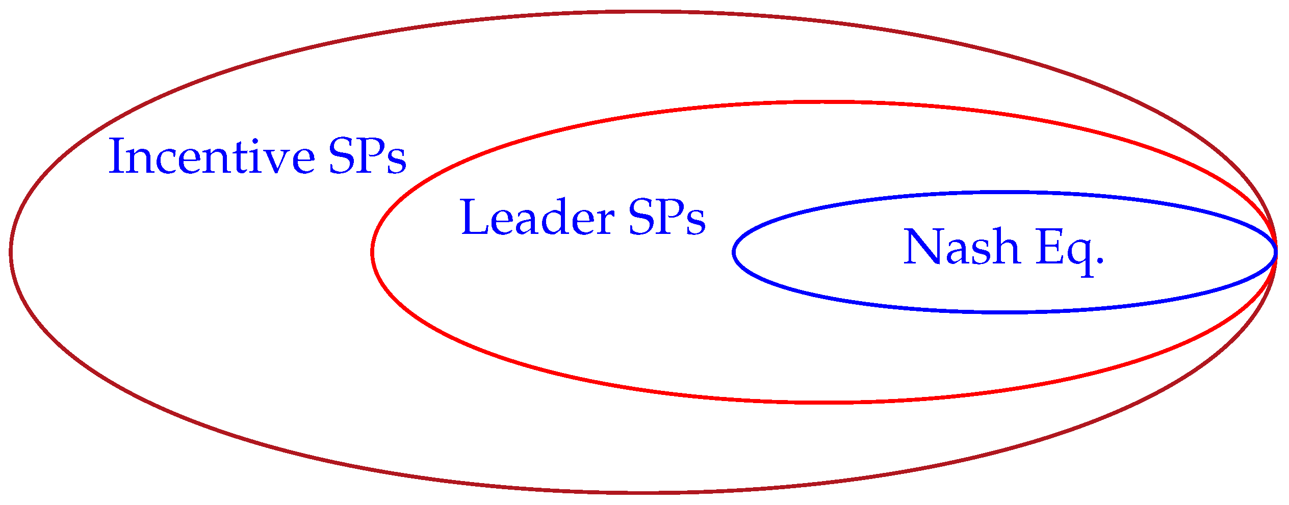
Table 1.
Equilibria in a bi-matrix game.
| Player II | |||
|---|---|---|---|
| I | II | ||
| Player I | I | 5,0 | 0,1 |
| II | 0,0 | −1,0 | |
Table 2.
A bi-matrix game where Nash and leader equilibrium are not same.
| Player II | |||
|---|---|---|---|
| I | II | ||
| Player I | I | 1,2 | 3,0 |
| II | 0,0 | 2,1 | |
Table 3.
Prisoner’s Dilemma.
| Player II | |||
|---|---|---|---|
| I | II | ||
| Player I | I | −1,−1 | −10,0 |
| II | 0,−10 | −8,−8 | |
Table 4.
An example where the follower does not benefit from incentive equilibrium.
| Player II | |||
|---|---|---|---|
| I | II | ||
| Player I | I | 1,2 | 0,0 |
| II | −10,1 | 10,0 | |
Table 5.
Leader behaves in a friendly way when her follower is also friendly.
| Follower | |||
|---|---|---|---|
| I | II | ||
| Leader | I | 1,0 | 0,0 |
| II | 1,1 | 1,1 | |
Table 6.
A travel agent scenario.
| Airline | Agent-Value | Customer-Value |
|---|---|---|
| Air India: | $100 | $170 |
| German Wings: | $50 | $100 |
| Lufthansa: | $120 | $80 |
| Ryan Air: | $5 | $200 |
| US Airways: | $100 | $150 |
Table 7.
A variant of the prisoner’s dilemma.
| Prisoner II | |||
|---|---|---|---|
| C | D | ||
| Prisoner I | C | 0,1 | |
| D | 1,0 | ||
Table 8.
A Battle-of-Sexes game.
| Player II | |||
|---|---|---|---|
| I | II | ||
| Player I | I | 1,2 | 0,0 |
| II | 0,0 | 2,1 | |
Table 9.
A simple bi-matrix game without a secure incentive equilibrium.
| Follower | |||
|---|---|---|---|
| I | II | ||
| Leader | I | 1,0 | 0,0 |
Table 10.
A variant of Battle-of-Sexes game.
| Player II | ||||
|---|---|---|---|---|
| I | II | III | ||
| Player I | I | 1,3 | 0,0 | 4,2 |
| II | 0,0 | 3,1 | 3,−3 | |
Table 11.
An example where is empty.
| Player II | |||
|---|---|---|---|
| I | II | ||
| Player I | I | 0,1 | 1,1 |
Table 12.
Values using continuous payoffs in the range 0 to 1.
| Incentive Equilibria | Leader Equilibria | |||||||||||
|---|---|---|---|---|---|---|---|---|---|---|---|---|
| #FSt | #LSt | Lead R | Foll R | Bribery | conf I | conf I | ET | Lead R | Foll R | conf I | conf I | ET |
| average | average | average | leader | follower | (minutes) | average | average | leader | follower | (minutes) | ||
| 2 | 2 | 0.726498 | 0.621347 | 0.031252 | 0.001188 | 0.001705 | 4.2175 | 0.698048 | 0.612999 | 0.001332 | 0.001774 | 2.7368 |
| 2 | 3 | 0.798458 | 0.585959 | 0.020400 | 0.000926 | 0.002014 | 4.6354 | 0.785525 | 0.577285 | 0.001009 | 0.002068 | 3.8177 |
| 2 | 5 | 0.868985 | 0.529380 | 0.010426 | 0.000642 | 0.002537 | 4.5459 | 0.865601 | 0.523492 | 0.000667 | 0.002555 | 4.0808 |
| 2 | 10 | 0.929643 | 0.434452 | 0.003310 | 0.000365 | 0.003249 | 6.4351 | 0.929367 | 0.432039 | 0.000367 | 0.003250 | 4.5798 |
| 3 | 2 | 0.752211 | 0.697569 | 0.043221 | 0.001051 | 0.001526 | 5.0878 | 0.710645 | 0.683939 | 0.001274 | 0.001623 | 4.5323 |
| 3 | 3 | 0.818569 | 0.662023 | 0.027266 | 0.000809 | 0.001893 | 6.5401 | 0.800711 | 0.647836 | 0.000926 | 0.001970 | 4.9813 |
| 5 | 3 | 0.856830 | 0.558777 | 0.026226 | 0.000646 | 0.003482 | 11.1242 | 0.817277 | 0.725141 | 0.000843 | 0.001852 | 8.0363 |
| 10 | 10 | 0.967437 | 0.184819 | 0.003880 | 0.000160 | 0.005209 | 35.8585 | 0.954231 | 0.684151 | 0.000207 | 0.003089 | 34.0453 |
Table 13.
Values using integer payoffs in the range −10 to 10.
| Incentive Equilibria | Leader Equilibria | |||||||||||
|---|---|---|---|---|---|---|---|---|---|---|---|---|
| #FSt | #LSt | Lead R | Foll R | Bribery | conf I | conf I | ET | Lead R | Foll R | conf I | conf I | ET |
| average | average | average | leader | follower | (minutes) | average | average | leader | follower | (minutes) | ||
| 2 | 2 | 4.748595 | 3.030555 | 0.661109 | 0.024802 | 0.030519 | 3.5780 | 4.227947 | 2.982509 | 0.027691 | 0.030597 | 3.5780 |
| 2 | 3 | 6.272594 | 2.880576 | 0.432742 | 0.019294 | 0.030389 | 3.9091 | 6.041986 | 2.797888 | 0.020913 | 0.030337 | 3.3044 |
| 2 | 5 | 8.723898 | 2.894013 | 0.217244 | 0.013183 | 0.029920 | 4.1927 | 7.666887 | 2.831469 | 0.013692 | 0.029740 | 3.3426 |
| 2 | 10 | 8.982101 | 3.039720 | 0.068128 | 0.006878 | 0.029555 | 4.9849 | 8.977945 | 3.013178 | 0.006930 | 0.029482 | 4.1737 |
| 3 | 2 | 5.295267 | 4.623187 | 0.901498 | 0.021894 | 0.025617 | 4.9897 | 4.552556 | 4.473518 | 0.026218 | 0.025743 | 3.6521 |
| 3 | 3 | 6.680038 | 4.444846 | 0.575029 | 0.016841 | 0.025512 | 5.3623 | 6.356434 | 4.286942 | 0.019193 | 0.025418 | 3.9804 |
| 5 | 3 | 7.4977325 | 6.740712 | 0.548419 | 0.013251 | 0.032891 | 7.6684 | 6.728477 | 5.887561 | 0.017346 | 0.019969 | 5.7481 |
| 10 | 10 | 9.727398 | 7.82520 | 0.065963 | 0.002783 | 0.046590 | 37.3025 | 9.41755 | 7.587172 | 0.003934 | 0.013824 | 24.9537 |
Table 14.
Average leader return and follower return in different equilibria.
| Leader Return | Follower Return | |||||||
|---|---|---|---|---|---|---|---|---|
| #FSt | #LSt | Incentive | Leader | Nash | Incentive | Leader | Nash | |
| 2 | 2 | 5.96 | 4.28 | 1.34 | 0.56 | 5.24 | 4.05 | 3.53 |
| 2 | 3 | 6.13 | 4.78 | 2.45 | 0.54 | 3.77 | 2.61 | 1.9 |
| 2 | 5 | 5.33 | 5.33 | 2.81 | 0.48 | 2.87 | 0.94 | 0.14 |
| 2 | 10 | 8.81 | 8.81 | 7.1 | 0.66 | 5.69 | 5.26 | 1.89 |
| 3 | 2 | 4.93 | 3.43 | 1.23 | 0.54 | 5.31 | 5.3 | 5.3 |
| 3 | 3 | 5.94 | 4.71 | 0.67 | 0.57 | 5.56 | 4.3 | 4.3 |
| 5 | 3 | 5.95 | 4.34 | 1.12 | 0.52 | 6.24 | 6.12 | 5.2 |
| 10 | 10 | 9.13 | 9.01 | 6.72 | 0.78 | 7.27 | 6.7 | 1.96 |
Table 15.
An example where the follower does not benefit from incentive eqilibrium.
| Player II | |||
|---|---|---|---|
| I | II | ||
| Player I | I | a,b | c,d |
| II | e,f | g,h | |
Table 16.
Loss of inconsiderate followers.
| Follower | |||
|---|---|---|---|
| I | II | ||
| Leader | I | 1,1 | 0,1 |
| II | 1,0 | −1,−1 | |
© 2018 by the authors. Licensee MDPI, Basel, Switzerland. This article is an open access article distributed under the terms and conditions of the Creative Commons Attribution (CC BY) license (http://creativecommons.org/licenses/by/4.0/).
Share and Cite
MDPI and ACS Style
Gupta, A.; Schewe, S. Buying Optimal Payoffs in Bi-Matrix Games. Games 2018, 9, 40. https://0-doi-org.brum.beds.ac.uk/10.3390/g9030040
AMA Style
Gupta A, Schewe S. Buying Optimal Payoffs in Bi-Matrix Games. Games. 2018; 9(3):40. https://0-doi-org.brum.beds.ac.uk/10.3390/g9030040
Chicago/Turabian StyleGupta, Anshul, and Sven Schewe. 2018. "Buying Optimal Payoffs in Bi-Matrix Games" Games 9, no. 3: 40. https://0-doi-org.brum.beds.ac.uk/10.3390/g9030040
Note that from the first issue of 2016, this journal uses article numbers instead of page numbers. See further details here.