An Automated Method for Building Cognitive Models for Turn-Based Games from a Strategy Logic


1
Department of Artificial Intelligence, Bernoulli Institute of Mathematics, Computer Science and Artificial Intelligence, University of Groningen, PO Box 407, 9700 AK Groningen, The Netherlands
2
Computer Science Unit, Indian Statistical Institute, 110 Nelson Manickam Road, Chennai 600029, India
*
Author to whom correspondence should be addressed.
Games 2018, 9(3), 44; https://0-doi-org.brum.beds.ac.uk/10.3390/g9030044
Submission received: 18 May 2018
/
Revised: 2 July 2018
/
Accepted: 4 July 2018
/
Published: 6 July 2018
(This article belongs to the Special Issue Logic and Game Theory)
Abstract
:Whereas game theorists and logicians use formal methods to investigate ideal strategic behavior, many cognitive scientists use computational cognitive models of the human mind to predict and simulate human behavior. In this paper, we aim to bring these fields closer together by creating a generic translation system which, starting from a strategy for a turn-based game represented in formal logic, automatically generates a computational model in the Primitive Information Processing Elements (PRIMs) cognitive architecture, which has been validated on various experiments in cognitive psychology. The PRIMs models can be run and fitted to participants’ data in terms of decisions, response times, and answers to questions. As a proof of concept, we run computational modeling experiments on the basis of a game-theoretic experiment about the turn-based game “Marble Drop with Surprising Opponent”, in which the opponent often starts with a seemingly irrational move. We run such models starting from logical representations of several strategies, such as backward induction and extensive-form rationalizability, as well as different player types according to stance towards risk and level of theory of mind. Hereby, response times and decisions for such centipede-like games are generated, which in turn leads to concrete predictions for future experiments with human participants. Such precise predictions about different aspects, including reaction times, eye movements and active brain areas, cannot be derived on the basis of a strategy logic by itself: the computational cognitive models play a vital role and our generic translation system makes their construction more efficient and systematic than before.
1. Introduction
Many events that happen in our daily life can be thought of as turn-based games. In fact, besides the “games” in the literal sense, our day-to-day dialogues, interactions, legal procedures, social and political actions, and biological phenomena—all these can be viewed as games together with their goals and strategies. Thus, effective and efficient strategies are needed everywhere, not just in games such as chess and bridge, but also in many social interactions in daily life, as well as other global phenomena and scientific procedures. For example, consider negotiations among rival parties to attain certain goals satisfactory to all, stabilization of entering firms in existing markets and decisions regarding an ideal situation to approach somebody for business. On an even larger scale, strategies are also of vital importance in negotiations in international crisis cases such as the Cuba missile crisis, the North Korean crisis, and Copenhagen climate change control. In biology, studying strategies is an important part of investigations of evolution and stabilization of populations.
Since strategies influence our daily lives as well as our broader existence in so many different ways, the study of strategies has become an integral part of many areas of science: game theory itself; ethics and social philosophy; the study of multi-agent systems in computer science; evolutionary game theory in biology; strategic reasoning in cognitive science; and the study of meaning in linguistics. There are various signs of interdisciplinary cooperation between these fields based on the basic similarities between the perspectives on strategies, and our current study is an example of this cooperation from the viewpoints of logic and computational cognitive modeling. The focus is on human strategic behavior.
In game theory (cf. [1]), strategies and their dependence on information form the main topics of study. One focus of study is on strategies bringing about equilibrium play in competitive as well as cooperative situations. Many important concepts, such as Nash equilibrium, sub-game perfect equilibrium, sequential equilibrium and extensions and modifications thereof have been developed over the years by game theorists while modeling various situations as games [1]. From the viewpoint of logical studies, modeling social interaction has brought to the fore various formal systems to model agents’ knowledge, beliefs, preferences, goals, intentions, common knowledge and common belief [2,3,4]. While modeling intelligent interaction, logicians have been interested in the questions of how an agent selects a particular strategy, what structure strategies may have, and how strategies are related to information [5,6,7]. In contrast to the idealized game-theoretic and logical studies on strategies in interactive systems, which assume the interactive agents to be “rational”, many experiments (e.g., see [8,9,10]) have shown that people are not completely rational in the sense of maximizing their current utilities. Players may be altruists, giving more weight to the opponent’s payoff; or they may try to salvage a good cooperative relation in the case they meet the other agent again in the future1. There might be cognitive constraints as well, such as working memory capacity [15,16], because of which the players are unable to perform optimal strategic reasoning, even if in principle they are willing to do so.
In fact, strategic reasoning in complex interactive situations consists of multiple serial and concurrent cognitive functions, and thus it may be prone to great individual differences. Cognitive scientists construct fine-grained theories about human reasoning strategies [17,18], based on which they construct computational cognitive models. These models can be validated by comparing the model’s predicted outcomes to results from experiments with human subjects. They aim to explain certain aspects of cognition by assuming only general cognitive principles. Cognitive models can be broken down into mechanisms and thus one can focus on the basic cognitive functions, their properties and their combinations [19]. One can also compare the model’s output with human data, and acquire a better understanding of individual differences.
In [20,21], Ghosh, Verbrugge and other authors investigate how formal models and cognitive models can aid each other to bring about a more meaningful model of real-life scenarios. Here, formal models are used to describe actual human behavior, and not just ideal game-theoretic rationality. Game experiments lead to the behavioral strategies of humans in turn-based games among others. Such strategies can be modeled as logical formulas constituting a descriptive logic of strategies, which help in the construction of cognitive models. The cognitive models predict human behavior, which can be tested against the human data available from the experiments. The first actual computational cognitive models based on logical formulas were provided in [21], which were made in an ad hoc way, based on some heuristic strategies.
In this paper, we provide a translation system that, starting from a strategy represented in formal logic, automatically generates a computational model in a cognitive architecture, which can then be run to generate decisions made in certain games, e.g., perfect-information games in our case. The formal strategies that we use describe a range of possible player types and behaviors, not just idealized behavior. Our main objective is to help understand human behavior. Our place in this body of research can be found in Figure 1. In Figure 1, human behavior is found at the top of the diagram. Based on this human behavior, game theorists formalize strategies that human participants may be using. Cognitive scientists can then use these formal strategies to manually construct cognitive models. These models can be used to automatically generate data, such as response times, decisions, neurological measures and simulated eye-tracking data. The behavior of such a model can be verified by, or provide predictions for, behavioral experiments, which can be used to obtain data on human behavior, closing the circle. In this diagram, dashed lines are automated processes. The red dashed line is our current research, which automates the creation of cognitive models from formal strategies. The blue line is the classical method of creating cognitive models by hand, based on observed human behavior.
Our translation system has been developed based on centipede-like games, a particular kind of perfect-information games. The choice of these games is not a matter of necessity but rather of convenience. Since we wanted to make predictions about experiments such as those reported in [9,10] which are based on centipede-like games, we concentrate on these games—the games that we base our discussions on are provided in Figure 2. These games are similar to centipede games (cf. Game 2 in Figure 2) in almost all respects, the only difference being that, unlike centipede games, the sum of the points of players may not increase in the subsequent moves [22]. The logic presented in Section 2 deals with strategic reasoning in any perfect-information game, not just the centipede-like games that we discuss here, and the translation method would work in principle for any finite binary perfect-information game, with at most two choices at each decision point.
A natural question to ask here is this: How would a translation method from strategy formulas to cognitive models help in the research on logic and game theory? Various logics of strategic reasoning in various forms of games have been developed until date, where elegant methods have been proposed to express and study properties of strategic reasoning (see, e.g., [23]). However, when it comes to human strategic reasoning, the formal systems can only express possible ways of doing strategic reasoning (cf. Section 2), without being able to pinpoint what actually happens. By this translation system, we are providing the next steps towards exploring the relation between the logical expressions and human behavior via cognitive models which provide us with both model behavior and reaction times which we can match with the human data to give a better understanding of these logical formulas in terms of expressing human strategic behavior. Our aim is to provide cognitive models of various strategies and reasoning types from the literature, namely, backward induction (BI) [1], extensive-form rationalizability (EFR) [24], different levels of theory of mind [25], and stances towards risk [25]. We take off from empirical studies with adults, focusing on these strategies and player types [9,10]. With these cognitive models corresponding to strategy and type specifications, we are all set to make predictions about human strategic reasoning based on logical formulas via the behavior of the corresponding cognitive models, which can be seen as “virtual participants”. From the cognitive modeling perspective, the logical formulas provide a systematic, exhaustive list of possibilities corresponding to each kind of strategic behavior, which aids in the development of these cognitive models that have been constructed hitherto in ad hoc ways.
In the next section, we present a strategy logic framework from [21] in terms of a strategy specification language which is used in the translation method. In Section 3, we present the translation system from strategy specifications to computational cognitive models. In Section 4, we perform various verification and exploratory experiments to verify the translation system and to discuss the behavior of the generated cognitive models in terms of their decisions and response times. We conclude in Section 5 with a discussion of our findings and some predictions about human strategic behavior.
2. A Strategy Logic
In [20], Ghosh et al. used a logical framework as a bridge between experimental findings and computational cognitive modeling of strategic reasoning in a simple Marble Drop setting, in which the computer opponent always made rational choices: “Marble Drop with Rational Opponent” (see Figure 3). Following this line of work, in [21], Ghosh et al. proposed a logical language specifying strategies as well as reasoning types of players that use empirical studies to provide insights into cognitive models of human strategic reasoning as performed during the experiment discussed in [26]. The marble drop setting was slightly different from the previous one—the computer opponent sometimes made surprising choices at the beginning, not adhering to rational choices all the time: “Marble Drop with Surprising Opponent”. The underlying games of this setting include the games given in Figure 2, with the computer opponent starting in Games 1–4 and playing b sometimes in Games 1 and 2, instead of the rational choice a.
For the purpose of the current work, we consider the logic as proposed in [21]. For ease of reference, we now provide a detailed description of the syntax and semantics of the logic, starting with certain concepts necessary for describing strategies and typologies.
2.1. Describing Game Trees and Strategies
In this subsection, we give definitions of extensive form games, game trees and strategies. Based on these concepts, we present the logic from [21] (with permission) in Section 2.2, where reasoning strategies and typologies are formalized.
2.1.1. Extensive Form Games
Extensive form games are a natural model for representing finite games in an explicit manner. In this model, the game is represented as a finite tree where the nodes of the tree correspond to the game positions and edges correspond to moves of players. For this logical study, we focus on game forms, and not on the games themselves, which come equipped with players’ payoffs at the leaf nodes of the games. The formal definition is presented below.
Let N denote the set of players, and let us restrict our attention to two player games, taking , C for computer and P for participant. The notation i and is often used to denote the players, where and . Let be a finite set of action symbols representing moves of players; let range over . For a set X and a finite sequence , let denote the last element in this sequence.
2.1.2. Game Trees
Let be a tree rooted at on the set of vertices S and let be a partial function specifying the edges of the tree. The tree is said to be finite if S is a finite set. For a node , let for some . A node s is called a leaf node (or terminal node) if .
An extensive form game tree is a pair where is a tree. The set S denotes the set of game positions with being the initial game position. The edge function specifies the moves enabled at a game position and the turn function associates each game position with a player. Technically, one needs player labeling only at the non-leaf nodes. However, for the sake of uniform presentation, there is no distinction between leaf nodes and non-leaf nodes as far as player labeling is concerned. An extensive form game tree is said to be finite if is finite. For , let and let denote the set of all leaf nodes of .
A play in the game starts by placing a token on and proceeds as follows: at any stage, if the token is at a position s and , then player i picks an action which is enabled for her at s, and the token is moved to where . Formally, a play in is simply a path in such that for all , . Let denote the set of all plays in the game tree .
2.1.3. Strategies
A strategy for player i is a function which specifies a move at every game position of the player, i.e., . For , the notation is used to denote strategies of player i and to denote strategies of player . By abuse of notation, the superscripts are dropped when the context is clear and the convention that represents strategies of player i and represents strategies of player is followed. A strategy can also be viewed as a subtree of where for each node belonging to player i, there is a unique outgoing edge and for nodes belonging to player , every enabled move is included. Formally, the strategy tree is defined as follows: For and a player i’s strategy , the strategy tree associated with is the least subtree of satisfying the following property:
- .
- For any node ,
- −
- if then there exists a unique and action a such that , where and .
- −
- if then for all such that , we have .
- .
Let denote the set of all strategies for player i in the extensive form game tree . A play is said to be consistent with if for all we have that implies . A strategy profile consists of a pair of strategies, one for each player.
2.1.4. Partial Strategies
A partial strategy for player i is a partial function which specifies a move at some (but not necessarily all) game positions of the player, i.e., . Let denote the domain of the partial function . For , the notation is used to denote partial strategies of player i and to denote partial strategies of player . When the context is clear, the superscripts are not used. A partial strategy can also be viewed as a subtree of where for some nodes belonging to player i, there is a unique outgoing edge and for other nodes belonging to player i as well as nodes belonging to player , every enabled move is included.
Formally, a partial strategy tree is defined as follows: For and a player i (partial) strategy the strategy tree associated with is the least subtree of satisfying the following property:
- For any node ,
- −
- if and then there exists a unique and action a such that .
- −
- if ( and ) or then for all such that , we have .
A partial strategy can be viewed as a set of total strategies. Given a partial strategy tree for a partial strategy for player i, a set of trees of total strategies can be defined as follows. A tree if and only if
- if then for all , implies
- if then there exists a unique and action a such that .
Note that is the set of all total strategy trees for player i that are subtrees of the partial strategy tree for i. Any total strategy can also be viewed as a partial strategy, where the corresponding set of total strategies becomes a singleton set.
2.1.5. Syntax for Extensive Form Game Trees
Let us now build a syntax for game trees (cf. [5,7]). This syntax is used to parameterize the belief operators given below to distinguish between belief operators for players at each node of a finite extensive form game. Let N denote a finite set of players and let be a finite set of action symbols representing moves of players; let range over . Let be a finite set. The syntax for specifying finite extensive form game trees is given by:
where , , , and .
Given , define the tree generated by z inductively as follows (see Figure 4 for an example):
- : where , .(If z is of the form , then z represents a node, and represents a tree with a single node with i being the player playing at .)
- : Inductively we have trees where for , .Define where
- −
- ;
- −
- and for all j, for all , ;
- −
- .
(If z is of the form , then z represents a tree with root node , and represents a tree with the root node with i being the player playing at , actions connecting the root node with trees , respectively, where represents for each i.)
Given , let denote the set of distinct pairs that occur in the expression of z.
2.2. Strategy Specifications
The syntax of Section 2.1 has been used in [20] to describe empirical reasoning of participants involved in a simpler game experiment using “Marble Drop with Rational Opponent” [25,26,27]. The | main case specifies, for a player, which conditions she tests before making a move. In what follows, the pre-condition for a move depends on observables that hold at the current game position, some belief conditions, as well as some simple finite past-time conditions and some finite look-ahead that each player can perform in terms of the structure of the game tree. Both the past-time and future conditions may involve some strategies that were or could be enforced by the players. These pre-conditions are given by the syntax defined below.
For any countable set X, let (the boolean, past and future combinations of the members of X) be sets of formulas given by the following syntax:
where , a countable set of actions.
Formulas in can be read as usual in a dynamic logic framework and are interpreted at game positions. The formula (respectively, ) refers to one step in the future (respectively, past). It asserts the existence of an a edge after (respectively, before) which holds. Note that future (past) time assertions up to any bounded depth can be coded by iteration of the corresponding constructs. The “time free” fragment of is formed by the boolean formulas over X. This fragment is denoted by .
For each and , a new operator is added to the syntax of to form the set of formulas . The formula can be read as “in the game tree z, player i believes at node x that holds”. One might feel that it is not elegant that the belief operator is parametrized by the nodes of the tree. However, our main aim is not to propose a logic for the sake of its nice properties, but to have a logical language that can be used suitably for constructing computational cognitive models corresponding to participants’ strategic reasoning.
2.2.1. Syntax
Let be a countable set of observables for and . To this set of observables, two kinds of propositional variables are added to denote “player i’s utility (or payoff) is ” and to denote that “the rational number r is less than or equal to the rational number q”2. The syntax of strategy specifications is given by:
where . For a detailed explanation, see [20]. The basic idea is to use the above constructs to specify properties of strategies as well as to combine them to describe a play of the game. For instance, the interpretation of a player i’s specification where , is to choose move a at every game position belonging to player i where p holds. At positions where p does not hold, the strategy is allowed to choose any enabled move. The strategy specification says that the strategy of player i conforms to the specification or . The construct says that the strategy conforms to specifications and .
2.2.2. Semantics
Perfect-information games with belief structures are considered as models. The idea is very similar to that of temporal belief revision frames presented in [28]. Let with , where is an extensive form game tree, is a utility function. For each with , there is already a binary relation over S (cf. the connection between z and presented above). Finally, is a valuation function. The truth value of a formula at the state s, denoted , is defined as follows:
- iff .
- iff .
- iff or .
- iff there exists an such that and .
- iff there exists an such that and .
- iff the underlying game tree of is the same as and for all such that , .
The truth definitions for the new propositions are as follows:
- iff .
- iff , where are rational numbers.
Strategy specifications are interpreted on strategy trees of . There are also two special propositions and that specify which player’s turn it is to move, i.e., the valuation function satisfies the property
- for all , iff .
One more special proposition is assumed to indicate the root of the game tree, that is the starting node of the game. The valuation function satisfies the property
- iff .
Recall that a strategy for player i is a function which specifies a move at every game position of the player, i.e., . A strategy can also be viewed as a subtree of where for each node belonging to the opponent player i, there is a unique outgoing edge and for nodes belonging to player , every enabled move is included. A partial strategy for player i is a partial function which specifies a move at some (but not necessarily all) game positions of the player, i.e., . A partial strategy can be viewed as a set of total strategies of the player [20].
The semantics of the strategy specifications are given as follows. Given a model M and a partial strategy specification , define a semantic function , where each partial strategy specification is associated with a set of total strategy trees and denotes the set of all player i strategies in the game tree .
For any , the semantic function is defined inductively:
- satisfying: iff satisfies the condition that, if is a player i node then implies .
Above, is the unique outgoing edge in at s. Recall that s is a player i node and therefore by definition of a strategy for player i, there is a unique outgoing edge at s.
Before describing specific strategies found in the empirical study, let us focus on the new operator of belief, proposed above. Note that this operator is considered for each node in each game. The idea is that the same player might have different beliefs at different nodes of the game. The syntax of extensive form game trees had to be introduced to make this definition sound, otherwise one would have had to restrict the discussion to single game trees.
Before ending this section, let us give an example regarding what can be expressed by the strategy specification language in terms of reasoning of the players. Letting refer to the j’th decision node, the formula describes the following strategy specification for player P in any of the games , with k varying from 1 to 4, mentioned in Figure 2: If the current node is accessible from the root node by the move b and P believes at node in the game that after the action d from the current node action f will be played, then play d. We note here that in the subformula , the action symbol f is taken as a formula—one can do so by adding all the action symbols as special propositions with their semantics given in an appropriate way.
3. Translation to Cognitive Models
In Section 2, we explain the logic from [21] that we use to express strategies in centipede-like games. Our translation system uses this logic to generate cognitive models in the PRIMs cognitive architecture. Before we explain this translation process and the behavior of these cognitive models, we give a brief overview of the PRIMs cognitive architecture [29].
3.1. The PRIMs Cognitive Architecture
PRIMs, short for “primitive information processing elements”, is a cognitive architecture that arose from the ACT-R cognitive architecture [19,30]. PRIMs is used to build computational cognitive models that simulate and predict human behavior in behavioral tasks. PRIMs models can be used to generate response times, decisions, eye movements, and activation in the brain. PRIMs is a modular architecture, consisting of five modules: a task control, manual, visual, declarative memory, and working memory module. These modules can be found in Figure 5. Each of these modules corresponds to an area in the brain, and all modules can work in parallel. Communication between these modules is performed using primitive elements, which either move or compare small pieces of information. Models in PRIMs are composed entirely of these primitive elements.
The manual module is used to perform actions, such as playing a move in a centipede-like game. The visual module is used to perform eye movements, retrieve information from a display, as well as to compare such information. Working memory is used for short-term storage of information, and declarative memory is used for long-term storage of information. The cognitive model’s declarative memory also contains how primitive elements have to be “chained together” to perform a task. Information is retrieved from declarative memory using a “retrieval request”. Partial information is sent to declarative memory, and, if it is present, a complete package of information is “retrieved”. The declarative memory of a cognitive model starts empty, unless otherwise specified. The task control module determines which sequences of primitive elements are relevant in the current stage of a task.
Models in the PRIMs cognitive architecture act as “virtual participants” and can play centipede-like games such as Game 1 in Figure 2. For example, a cognitive model can move its visual attention across edges in the game tree to look at payoffs, store these payoffs in working memory to remember them, or make comparisons between these payoffs by sending them to declarative memory and retrieving whether one is bigger or smaller, as our cognitive models’ declarative memory contains basic information about order relations of natural numbers.
Packages of information in declarative memory are called “chunks”, and each chunk has an activation value. This activation corresponds to how well it is remembered. A chunk’s activation decreases over time, and increases with usage of the chunk. When the activation of a chunk falls below the activation threshold, it can no longer be retrieved, and is forgotten. The implementation of activation in PRIMs corresponds to the findings of [31].
3.2. Representations
Our new translation system automatically generates a model in the PRIMs cognitive architecture from a formal strategy and the game it corresponds to. Within our system, centipede-like games are represented using the same tree structure shown in Figure 2. In this representation, games consist of nodes and edges. Nodes can be leaf nodes (ending locations) and non-leaf nodes (player turns). For leaf nodes, both players’ payoffs are specified. For non-leaf nodes, the player who has a turn at the node is specified. Edges specify the two nodes they connect. All finite centipede-like games can be stored in this manner.
Formal strategies, as represented in our system, differ in several ways from those in Section 2. Belief operators no longer specify which game they correspond to, as the game itself is already part of the system’s input. For readability, we still include the game in any formula. Furthermore, a comparison does not specify which payoffs are being compared, only which two natural numbers (including zero) are being compared. A game containing identical payoffs at different nodes poses a problem for a translation system. Although humans can intuitively determine which comparison would “make sense”, a translation system cannot. Because of this, we use a modified version of the formal logic where each payoff is marked, and each comparison refers to two specific payoffs. This allows a translation system to know precisely which two payoffs it has to pull from working memory to perform a comparison. We do not consider negated formulas in the translation system. This could be done by utilizing an exhaustive list of strategy formulas for each game. We were able to find such an exhaustive list of strategies thanks to the finiteness of the games. In addition, because all games considered here are binary, not choosing one alternative is equivalent to choosing the other one.
3.3. Low-Level Cognitive Model Behavior
Formal strategies, as represented in our system, consist of a player, an action, and a conjunction of conditions, stored in a list. Each of these conditions consists of a list of zero or more operators (such as ), and a proposition (such as ). These operators and propositions are represented in our system the same way they are in the logic: operators of the type consist of an edge and a boolean specifying their direction, and a belief operator contains a player name and a node. The proposition root contains no further information; turn contains a player; a utility specifies a player and the value q; and a comparison refers to two existing utilities. Edges in the game tree are used for actions, which are required both by the strategies and to formulate beliefs such as (Player C’s belief at the first decision node in Game 1 of Figure 2). An exhaustive strategy formula for a game is simply a list of all possible strategies for the game.
Given a centipede-like game and an exhaustive strategy formula, our system generates a model in the PRIMs cognitive architecture. We explain these cognitive models by first explaining what they will do given a single operator or proposition.
and
Sequences of these operators specify the location in the game tree where a proposition should be verified. A translated PRIMs model moves its visual attention towards this location, across the edges in the game tree, whenever it has to verify the proposition that follows them.
root
The PRIMs model will visually inspect the specified node to determine whether it is the root of the tree.
turn
The PRIMs model will read the player name of the player whose turn it is from the specified node in the game tree, and compare it to i.
The PRIMs model will compare to a value in its visual input when looking at the specified node. Because this value may be required for future comparisons, it is also stored in an empty slot of working memory.
A PRIMs model cannot instantly access each value in a visual display: it has to move its visual attention to them and remember them by placing them in working or declarative memory before it can compare them. A proposition causes such a value to be stored in working memory. A proposition then sends two of these values from working memory to declarative memory, to try and remember which one is bigger. When a cognitive model is created, its declarative memory is filled with facts about single-digit comparisons, such as and .
and a
The operator and proposition a are used to construct beliefs about the opponent’s strategy. To verify a belief formula such as , a cognitive model employs a strategy similar to the ones used by cognitive models in [32]. When a cognitive model is created, it contains several strategies in its declarative memory, both for Player P and Player C. When a cognitive model verifies a belief, it sends a partial (or empty) sequence of actions to declarative memory, corresponding to the assumptions of the belief, in an attempt to retrieve a full sequence of actions, which is a strategy. In the formula , Player C at node in Game 1 of Figure 2 believes that Player P will play c after its playing b, so a strategy for Player P will be retrieved. The formula assumes that Player C has played b, but makes no assumptions about Player P, because P has not yet played any action at this point in the game. Because no assumptions are made about Player P, no constraints are placed on the strategy that may be retrieved for Player P, so an empty strategy for P is sent to declarative memory. The sequences that could be retrieved based on these constraints depend on the game and strategy. For example, for BI in Game 1, the sequences c;g and c;h can be retrieved, as those are the BI strategies in Game 1 according to Table 1. Both of these sequences will verify , as both contain the action c that the formula is trying to verify.
The declarative memory of our PRIMs models can contain action sequences corresponding to the backward induction (BI) and extensive-form rationalizable (EFR) strategies, generated using the procedure from [33], as well as sequences corresponding to the own-payoff strategy, which simply specifies that you should play the actions along a path that leads to your highest payoff. These strategies can be found in Table 1.
3.4. High-Level Cognitive Model Behavior
We now explain the cognitive model behavior for a strategy formula. The strategy formulas we use as input for our system take the form of a Horn clause, such as . Here, p is true if all propositions in the conjunction are true. Given a strategy formula, a PRIMs model tries to verify each proposition in the conjunction sequentially, using the behavior described earlier for each proposition. If it encounters a proposition it cannot verify, it “jumps out of” this verification process and does not play the action prescribed by the formula (what it does we describe later). If the cognitive model has verified all the propositions in the conjunction, it plays the action prescribed by the strategy formula.
Conjunctions in formal logic are unordered, whereas models in PRIMs solve problems sequentially. Therefore, we need to order the conjunctions in formal logic, such that the corresponding PRIMs model has an order to verify them in. Fortunately, each proposition has to be verified at a specific location. For example, , in Game 1 found in Figure 2, has to be verified at the ending location reached by playing a. Eye-tracking data from [34] tells us that human participants tend to look through a game tree by following the edges along the shortest path. Therefore, we compute the shortest path through the game tree. Our PRIMs models verify propositions as they occur along this path. Another solution would be to use a non-commutative logic, for example, to use the non-commutative conjunction ⊙ proposed in [35]. Our present paper’s main focus lies on our translation system and not on an in-depth analysis of the logic we use, so it remains a possibility for future work to provide a logical syntax better suited for the translation system.
Exhaustive strategy formulas consist of one or more of such strategies, which are represented in our translation system as a list of multiple strategy formulas. A PRIMs model generated from this list tries to verify each formula in it, using the behavior described in the Section 3.3, until it finds one it can verify, and plays the action prescribed by the formula it verified. If it fails to verify each formula in the list, it will randomly play one of the available actions. Exhaustive strategy formulas are also unordered. Because of this, we take care that each possible order of the list of strategy formulas occurs the same number of times whenever we generate cognitive models or run cognitive models to obtain data.
4. Experiments and Results
To investigate our translation system, we run two sets of experiments: a set of verification experiments, and a set of exploratory experiments. In Section 4.1, we explain the models and experiments we use to verify our system, and present their results. In Section 4.2, we explain the methods used to run our exploratory experiments, and then present the results of each set of formulas separately.
4.1. Verification Experiments
We begin by running a set of verification experiments designed to compare cognitive models generated by our translation system to cognitive models made by hand. We perform our verification experiments using the so-called “myopic” and “own-payoff” strategies (see [21]). A player using the myopic strategy only looks at her own payoffs at the current and next leaf nodes, and moves towards the highest one. A player using the own-payoff strategy only looks at her own payoffs at her current and any future leaf nodes, and moves towards the highest one.
4.1.1. Methods
We create myopic and own-payoff cognitive models by hand, which perform the above strategy, and we also let our translation system generate a myopic and own-payoff cognitive model. The myopic and own-payoff models will only play Game 5 (cf. Figure 2). It is a truncated version of Games 1 and 2. We use this game for these strategies because the participant moves first here, instead of the computer. Indeed, when using the myopic or the own-payoff strategy, a participant does not take the computer’s first move into account at all.
We run each of these four models 48 times, to simulate 48 virtual participants. For the automatically generated models, we also run a separate batch of 1000 virtual participants, so we can investigate the models’ robustness. Each of these “participants” will play Game 5 for 48 times. Each model plays as Player P, and will only perform Player P’s first move in Game 5. Each trial ends when the model has played a move. We record response times and decisions made.
The formulas our myopic and own-payoff cognitive models are generated from are based on the myopic and own-payoff strategies. These formulas are for Game 5 only. They are as follows:
- ■
- Myopic, Game 5
- ■
- Own-payoff, Game 5
Note that these formulas are based on the myopic and own-payoff strategies, and not on the handmade myopic and own-payoff models. We feed these formulas to our translation system, which uses them to automatically generate new myopic and own-payoff models. These are the models we compare to our handmade models.
4.1.2. Results
We now present and discuss the results of our verification experiment. We begin by looking at the cognitive model’s decisions, and then look at the cognitive model’s response times.
Cognitive Model Behavior
The proportions that our myopic and own-payoff cognitive models play down, or c, can be found in Table 2. The automatically generated myopic and own-payoff cognitive models play according to the behavior described in Section 3. The handmade myopic and own-payoff cognitive models play according to the intuitive strategies described at the beginning of this Section 4.1: they use eye movements and declarative memory retrievals to find their highest payoff, either in the current and next leaf node when using the myopic strategy, or the current and every leaf node when using the own-payoff strategy. Both the strategies and the formulas prescribe that you should play down when using the myopic strategy, and right when using the own-payoff strategy. In short, the models’ behavior corresponds to the strategies they are using, and the correspondence between our handmade and generated models serves as verification for our translation system. There is no difference between the 48- and 1000-participant runs of the automatically generated models.
Response Times
Reaction times for the myopic and own-payoff cognitive models in Game 5 can be found in Figure 6. It can be seen that the own-payoff models have a bit under twice the response times of the corresponding myopic models. This is probably caused by the own-payoff models looking at two more payoffs in the game tree, and performing five more declarative memory retrievals when comparing payoff values. Both the handmade and generated models show the same difference between the myopic and own-payoff models, which serves as verification for our translation system. However, the generated models are faster than our handmade models. We believe this is because our handmade models are general to any centipede-like game, whereas the generated models are specific to Game 5: our generated models operate under the assumption that they are playing Game 5, so do not have to perform extra checks to adapt to the game they are playing. There is little difference between the 48- and 1000-participant runs of the automatically generated models, except that the error bars are larger for the 48-participant runs, which is to be expected.
4.2. Exploratory Experiments
In Section 4.1, we have verified our translation system by showing that the results of our handmade myopic and own-payoff cognitive models are very similar to myopic and own-payoff cognitive models that were automatically generated using our translation system. In the present section, we first describe a general method we use for our exploratory experiments, after which we alternate between presenting the formulas we use to generate cognitive models and the results we obtain from those cognitive models.
Almost all of the cognitive models in our exploratory experiments play Games 1–4 as found in Figure 2. There is one model for each game, for each strategy. We run each of these models 48 times, to simulate 48 virtual participants. Each of these “participants” plays their game 48 times. Each model plays as Player P, and will only perform Player P’s first move in their respective game, where Player C has already played b. Each trial ends when the model has played a move. We record response times and decisions made.
We now generate the cognitive models for the exploratory experiments from strategy formulas based on BI, EFR, theory-of-mind, and risk-aversiveness. We also create a cognitive model by hand which uses the BI procedure for games with and without payoff ties [33,36]. For theory-of-mind, we create cognitive models using zero-, first- and second-order theory-of-mind. The risk-based cognitive models attribute risk-aversiveness and risk-seeking to either Player P or C, for four risk-based cognitive models in total. The BI and EFR formulas are based on formal strategies, whereas the theory-of-mind and risk-based models are formulas based on types of behavior. For each of these strategies and types, we give one or more example formulas. The remainder of these formulas can be found in Appendix A.
All cognitive models start with comparison facts between the natural numbers one and six in their declarative memory, as these are the numbers relevant to the games under consideration. An example of such a fact is “one is smaller than four”. All cognitive models play as Player P, in a game where Player C has already played b. They do not play P’s second action. Each cognitive model is counterbalanced in terms of the order of strategy formulas within the exhaustive strategy formula it was generated from.
Because almost all of the formulas we use contain the conjunction , we abbreviate this conjunction as . Here, is defined as (adapted from [10]), where
- (from the current node, a d move followed by an f move followed by an h move lead to the payoff )
- (from the current node, a d move followed by an f move followed by a g move lead to the payoff )
- (from the current node, a d move followed by an e move lead to the payoff )
- (from the current node, a c move leads to the payoff )
- (the current node can be accessed from another node by a b move from where an a move leads to the payoff )
and is used to denote the conjunction of all the order relations of the rational payoffs for player given in the game (from [21]). Since this description applies to Games 1–4, and our cognitive models play as Player P in her first move, the “current node” refers to the second node in the game tree, with outgoing edges c and d. For the ease of reading, in the formulas above and those in the rest of the paper, we have used the operator symbol to mean the operator , for any action symbol x.
In the remainder of this section, we alternate between providing strategy formulas used to generate cognitive models, and presenting the results of those models when used in the experiment described above. We begin with the strategies BI and EFR.
4.2.1. Backward Induction and Extensive-Form Rationalizability
Models
Our first batch of cognitive models are based on the BI and EFR strategies. Apart from the BI and EFR cognitive models that we generate from their strategy formulas, we also create a BI cognitive models by hand, which uses the BI procedure as presented in [20]. The BI formulas we use to generate cognitive models are based on the BI strategies as found in Table 1. We give example formulas for Games 1 and 3 as found in Figure 2. In Game 1, there is one BI solution, so the exhaustive strategy formula consists of one formula. In Game 3, there are two BI solutions, so the exhaustive strategy formula consists of two formulas. The BI cognitive models only have BI beliefs in their declarative memory, corresponding to the first column of Table 1. The exhaustive strategy formulas for BI in Games 1 and 3 are as follows:
- ■
- Backward induction, Game 1
- ■
- Backward induction, Game 3
The cognitive models generated from the BI formulas only have BI beliefs in their declarative memory. The exhaustive EFR formulas are constructed in the same manner as the BI formulas. The EFR cognitive models only have EFR beliefs in their declarative memory. The EFR formulas for Games 1 and 3 are as follows:
- ■
- Extensive-form rationalizability, Game 1
- ■
- Extensive-form rationalizability, Game 3
The results we obtain when running the BI and EFR models, as described above, using the methods described at the start of this section, can be found in the next two paragraphs.
Results: Cognitive Model Behavior
The proportions that our BI and EFR cognitive models play down, or c, can be found in Table 3.
It can be seen that the handmade BI cognitive model always plays down in Games 1 and 2, and plays down about half the time in Games 3 and 4. This is because using the BI procedure, there is only one BI solution in Games 1 and 2, which is playing down, and because of the payoff ties in Games 3 and 4, there are two BI solutions, one prescribing to play down, while the other prescribes right.
The proportions down played in Games 1 and 2, for both BI and EFR, are all close to 0.5. As mentioned, the cognitive models sequentially try to verify each of the propositions in the strategy formulas they were generated from. We assume cognitive models will always be able to verify , because only contains true facts about the game tree. Because of this, the cognitive model behavior is mostly dependent on the beliefs it has to verify. As mentioned, the cognitive model plays as Player P, after Player C has already played b. When verifying beliefs about C, this knowledge is used in trying to retrieve a strategy for Player C. Thus, every time a belief concerning C is verified in these cognitive models, the incomplete strategy b-? is sent to declarative memory, and either b-e or b-f is retrieved, or the cognitive model fails at retrieving a strategy because neither b-e or b-f are among its strategies in memory. As one can see in Table 1, no BI or EFR strategy in Games 1 and 2 starts with C playing b. Because of this, the cognitive models cannot verify their beliefs when playing Games 1 and 2, so they select randomly from down and right, which is why the proportions are all close to 0.5.
In more behavioral terms, the cognitive models for BI and EFR in Games 1 and 2 are trying to verify their corresponding strategies. However, the fact that C has already played b does not correspond to these strategies. The cognitive models are trying to play a strategy in a situation that contradicts this strategy, and hence cannot play corresponding to this strategy.
The proportions of down played in Game 4, for both BI and EFR, are also close to 0.5. However, since the BI and EFR strategies include strategies such as b;f and d;g, the cognitive models do have the opportunity to verify the beliefs in the formulas they were generated from. However, the strategy formulas for BI and EFR in Game 4 are symmetric with regard to the action that is prescribed: within the exhaustive strategy formula, there is an equal number of strategies that prescribe c as there are that prescribe d. Because of this, the proportions are close to 0.5.
Perhaps the most interesting game with regard to the strategy table (Table 1) is Game 3, because not all strategies are BI or EFR strategies, but there are strategies present such that the cognitive models can verify their beliefs. For example, in Game 3, b;e is not a BI strategy. Because of this, the belief that C will play e cannot be verified by the BI cognitive model. However, b;f is a BI strategy, so it can be verified. In Section 4.2.1, we have seen that there are two BI solutions in Game 3: in one, you always play down, but in the other, you always play right. According to the previous explanation, a cognitive model cannot verify the one where you always play down, because C has already played right in the current situation, so only one of these solutions corresponds to the current situation. Because of this, the cognitive model will play right more often than down.
The EFR cognitive models in Game 3 mostly play right. This is because both strategy formulas prescribe that the cognitive model should play right. The cognitive model first tries to verify the first formula. If it succeeds, it plays right. If it does not, it tries to verify the second formula. If it succeeds, it plays right. If it does not, it plays randomly, giving it a 0.5 probability to play right. Because of this, it is very unlikely that the EFR cognitive models in Game 3 play down, which we see in the proportions of playing down in Table 3.
Results: Response Times
Reaction times for the BI and EFR cognitive models, as well as the handmade BI cognitive model, in Games 1–4 can be found in Figure 7. For all BI and EFR cognitive models, there is no difference between Games 1 and 2 in terms of the strategy formulas as well as the BI procedure, which explains the lack of differences between Games 1 and 2. The handmade BI cognitive model does not look at the first leaf node, which is where Games 3 and 4 differ. This explains the lack of difference between Games 3 and 4 for the handmade BI cognitive model.
The handmade BI cognitive model is slightly faster at Games 3 and 4 than at Games 1 and 2. This is because of the payoff ties in Games 3 and 4: the cognitive model first compares values in the game tree by checking whether they are equal, and if they are not, it will send a retrieval request to declarative memory to determine which one is bigger. In short, the handmade BI cognitive models perform one less retrieval request in Games 3 and 4.
The BI and EFR cognitive models in Games 1 and 2 are faster than those in Games 3 and 4. This is because the BI and EFR cognitive models in Games 1 and 2 are generated from only one strategy formula: if this formula fails to verify, the cognitive model stops and plays randomly. As for Games 3 and 4, if the first formula fails, the corresponding cognitive models will move to the next formula. There seems to be a “ceiling” where response times do not increase much anymore. The EFR cognitive model in Game 4 is slower than the one in Game 3 because it consists of more formulas, but not by much.
Therefore, we believe that these cognitive models will, on average, succeed at verifying a formula approximately “two formulas in to the list”. This could be why response times are not a direct function of the number of formulas a cognitive model was generated from. The difference between the BI cognitive models in Games 3 and 4 have a different explanation: in Game 3, one of the BI formulas is impossible to verify, whereas, in Game 4, it is not. Because of this, the cognitive models playing BI in Game 3 will play down earlier more often.
4.2.2. Theory-of-Mind
Models
For the theory-of-mind cognitive models, the formulas we generate our cognitive models from are based on what order of theory-of-mind one is using. Zero-order theory-of-mind users do not consider the other player’s beliefs, whereas first-order theory-of-mind players consider the other player’s beliefs. Since any such beliefs correspond to theory-of-mind, the theory-of-mind formulas are the same for all Games 1–4. Because of this, we only show the exhaustive strategy formulas for theory-of-mind in Game 1. The theory-of-mind cognitive models have beliefs corresponding to the BI, EFR, and own-payoff strategies in their declarative memory.
- ■
- Zero-order theory-of-mind, Game 1
- ■
- First-order theory-of-mind, Game 1
- ■
- Second-order theory-of-mind, Game 1
We generate cognitive models from these formulas, and run them using the methods described at the beginning of Section 4.2. Our results are described in the next paragraph. Unlike in the other experiments, we do not look at cognitive model behavior for the theory-of-mind models, as all exhaustive strategy formulas are symmetric with regard to the action which is prescribed.
Results: Response Times
Response times for the automatically generated zero- to second-order theory-of-mind cognitive models in Games 1–4 can be found in Figure 8.
The theory-of-mind cognitive models are the same across Games 1–4, which explains why there is little difference among Games 1–4 within each order of theory-of-mind. The zero-order theory-of-mind cognitive models are much faster than the first- and second-order cognitive models. This is because the zero-order theory-of-mind cognitive models’ formulas only contains payoffs, comparisons, and root, and no beliefs. Because these propositions are about true facts about the game tree, verifying them will always succeed, so the zero-order theory-of-mind cognitive models will always play an action after successfully verifying their first formula.
There are two factors that explain the difference between the first- and second-order theory-of-mind cognitive models. First, first-order theory-of-mind cognitive models have to verify one belief per formula, whereas second-order theory-of-mind cognitive models have to verify two beliefs per formula. Secondly, exhaustive first-order theory-of-mind formulas consist of four formulas, whereas exhaustive second-order theory-of-mind formulas consist of eight formulas. However, as we have seen in the BI and EFR cognitive models, we believe the first- and second-order succeed at verifying a formula in the exhaustive strategy formulas approximately “the same number of formulas in”, which is why response times are not a function of number of formulas.
4.2.3. Risk-Based Models
Models
Our risk-based cognitive models only play Game 4. Their declarative memory is filled with strategies corresponding to BI, EFR, and own-payoff. There are four risk-based cognitive models: two where the cognitive model itself is risk-seeking or risk-averse, and two where the cognitive model attributes risk-seeking or risk-aversiveness to the other player, Player C. For example, if the cognitive model itself is risk-averse, it will play d if it believes Player C will play e.
- ■
- Risk-averse, P, Game 4
- ■
- Risk-seeking, P, Game 4
- ■
- Risk-averse, attributed to C, Game 4
- ■
- Risk-seeking, attributed to C, Game 4
Unlike the BI, EFR, and theory-of-mind models, the risk-based models will only play Game 4, using the methods described at the beginning of Section 4.2. Their results can be found below.
Results: Cognitive Model Behavior
The proportions that our risk-based cognitive models play down, or c, can be found in Table 4. The behavior of the risk-based cognitive models corresponds to the actions that are prescribed in the corresponding formulas. For example, in the risk-averse formula for P, the formula prescribes playing c, or down. The proportion close to 0.7 corresponds to this. However, perhaps the best way to explain the cognitive model behavior in the risk-based formulas is using probabilities. Consider the risk-averse cognitive models for P, which plays in Game 4. The formula it was generated from is . Since describes true facts about the game tree, we assume the probability of successfully verifying is 1. Because of this, what the cognitive model plays depends on the belief . To verify whether C will play e, the cognitive model will send the sequence of actions C has played before the current situation to declarative memory in an attempt to find a strategy where C plays e. This sequence is b-?, because C has played b. The declarative memory of the risk-based cognitive models contain BI, EFR, and own-payoff beliefs. Because the risk-based cognitive models play Game 4, the beliefs are simply the row corresponding to Game 4 in Table 1. Beliefs concerning P are not relevant for verifying , and beliefs starting with a are not retrieved because the cognitive model searches for a belief that starts with b. Because of all this, the list of beliefs it may retrieve consists of b;f, three times, and b;e, two times. Retrieving b;e will verify the cognitive model’s beliefs, retrieving b;f will falsify them. Therefore, the probability of verifying these beliefs is , so there is a 0.4 probability of successfully verifying the formula and playing c, the action it prescribes. On the other hand, there is a 0.6 probability the formula is falsified, in which case an action is played randomly. Thus, within this 0.6 probability, there is a 0.3 probability that c is played, and a 0.3 probability d is played. Add the probabilities that c will be played and you get 0.7, which is very close to the observed proportion of playing down by the risk-averse cognitive model for P, in Table 4 (recall that we round off to three digits).
Results: Response Times
Response times for the automatically generated risk-based cognitive models in Game 4 can be found in Figure 9. The response times for the risk-based cognitive models follow the same general tendencies we have seen in those for other automatically generated cognitive models. The “participant, risk-averse” cognitive model is fastest, probably because it only has to verify one belief. All other cognitive models have to verify two beliefs per formula. The “participant, risk-taker” cognitive model is slowest, probably because it consists of two formulas where all other exhaustive formulas consist of one formula. The risk-averse cognitive model for C could be slightly faster than the risk-taking cognitive model for C, because verifying is less likely than verifying , but this difference could also be coincidental.
4.3. General Findings
To explain the cognitive model behavior for the risk-based models, we used a method where we calculate the probability that a cognitive model will play a certain action, based on the strategy formulas it was generated from. In fact, most of the probabilities of playing c, obtained using this method, correspond rather nicely to the observed proportions of playing down. There are two important exceptions: EFR in Game 3, and the “risk-taker, P” cognitive model in Game 4. These cognitive models are generated from the same formulas, but have different beliefs. These formulas are and . What we found is that failing to verify the first formula “sets the cognitive model up” for succeeding in verifying the second one, in some cases. If is verified, then the chunk b-f would have been retrieved from memory, which increases this chunk’s activation. If fails, then d-h would have been retrieved instead of d-g, which increases the activation of d-h. Because the first formula fails, the cognitive model will try to verify the second one. With the activation of b-f and d-h increased, it is more likely it will retrieve these strategies, which are exactly the strategies required to verify the second formula. The same holds if the order of both formulas is exchanged.
Note that, although we ran a total of trials, we ran 48 “virtual participants” who played 48 trials each. The behavior on later trials is influenced by earlier trials. If on the first trial, a certain chunk is retrieved, or a certain action is played, this chunk or action will receive activation, which makes it much more likely to be used on later trials. Because of this, it is highly likely that within all 48 trials of a single virtual participant, when all other things are equal, the same behavior will occur. The mean response of 48 “different” observations is much more likely to deviate from an expected value, such as 0.5, than the mean response of 2304 observations. In short, if a BI cognitive model in Game 1 plays down on its first trial, it is very likely it will always play down in its 47 subsequent trials.
There are several tendencies we see in all cognitive models generated from the strategy formulas. For example, response times seem to increase as the number of strategy formulas within an exhaustive strategy formula increase. Response times also seem to increase as the number of beliefs within each strategy formula increase. Cognitive models are more likely to play the strategy prescribed by the strategy formulas they were generated from, except when the current state of the game—that is, Player C has played b—contradicts the strategy they are attempting to play. We elaborate on some of these findings in the next section.
5. Discussion and Conclusions
Logicians have long studied reasoning mainly from a prescriptive perspective, concentrating on questions such as which inferences are logically valid. Similarly, game theorists have long been mostly interested in the perspective of modeling strategies under the condition of commonly known rationality of the players. In the meantime, psychologists have performed many experiments showing that people often do not appear to reason correctly by the laws of classical logic [37]; and behavioral economists have shown that people do not play according to the Nash equilibrium [38]. Fortunately, over the last decade, more and more researchers from both the formal sciences and the behavioral sciences have attempted to combine forces to better explain reasoning and strategizing, realizing that facts matter to logic and game theory, and, on the other hand, that logic and game theory can help explain the facts [13,39,40,41,42,43]. The current study aimed to strengthen the bridge between these areas.
This article has as a starting point the logical language expressing strategies that people can apply when reasoning about their opponent and making decisions in turn-based games, such as the game Marble Drop with Surprising Opponent that we use here as an example. The language can express different possible strategies as well as reasoning types reflected in participants’ behavior and, in addition to referring to players’ actions, it can also represent their (higher-order) beliefs [21]. Similar to other logical approaches to strategies, the strategy logic cannot directly be used to model human strategic reasoning in turn-based games. After all, the logic does not explicitly say anything about aspects that have been found to be very useful in cognitive research on human strategic reasoning, such as eye movements (reflecting dynamic attention shifts during reasoning), reaction times, and active areas of the brain.
However, the logical language becomes very useful when the formulas are used to construct computational cognitive models, in our case in the cognitive architecture PRIMs. An important advantage of using PRIMs, rather than a computational model constructed from scratch, is that PRIMs implements precise, experimentally validated theories about human memory and cognitive bounds on reasoning processes. The logical strategy language of [21] helps to delineate a number of plausible reasoning strategies in a systematic manner, which can then be translated into computational models in PRIMs. The formulas are implemented as production rules, which handle visual processing (a participant gazing through the game tree), intermediate problem state updates, and motor processing.
Our translation system of Section 3 generates computational cognitive models from strategy formulas, without human intervention, in a generic way. This has the potential to greatly speed up cognitive research on strategic reasoning, because cognitive models have so far usually been created by hand, one by one. Our computational cognitive models can be run as a kind of virtual experimental participants, to obtain reaction times, as shown in our results, as well as other data, such as decisions, gazing behavior, and neural activity. The results in Section 4 show the feasibility of our system as a proof-of-concept.
5.1. Verification of the Automated Translation Method and Exploratory Experiments
Our verification experiment in Section 4 shows that, between the handmade and generated models, the proportion of reaction times between the myopic and own-payoff strategies are highly similar, indicating similarity in their decision-making processes. For example, in both the handmade and the automatically translated myopic model, the model looks at two payoffs in the game tree, stores them in memory, and compares them to make its decision. The difference in reaction times could be due to the fact that the automatically generated models are specific models for their respective games, each one geared to a specific payoff structure, whereas the handmade models are general models. Because of this, the handmade models have to perform extra tests to verify whether certain operations are possible in the current game, and they have to remember what they have already done. In contrast, the generated models are generated from a strategy formula designed for a particular game, so they can simply perform a sequence of actions.
The main problem that we encounter in our verification experiment is that the reaction times for the automatically translated cognitive models are too slow to resemble human reaction times, especially knowing that human participants probably use a more complex strategy than the own-payoff strategy, requiring even more processing steps. We believe that this is because of the relatively slow speed with which our models move their visual attention through the game tree, visiting each decision point and leaf from the root on to the right. The problem of being much slower than human participants does not occur in the simplistic handmade PRIMs models in [21], which are unrealistic in the sense that those “virtual participants” do no gazing whatsoever. The current exhaustive models do move their focus back to the root if one of the formulas from he exhaustive list fails to check the next one if available.
Focus actions are a relatively novel addition to PRIMs, having been added for [44], where response times are unused. This suggests that apart from “finding the strategy formula that best corresponds to human strategic reasoning”, we also need to further develop focus actions in PRIMs to be reminiscent of human gazing. Nonetheless, our verification experiment shows that our system can be used to make predictions.
In addition, we have performed simulation experiments based on computational cognitive PRIMs models, where we looked at both decisions and reaction times and compared different models on these aspects. We compared these aspects between a handmade model for BI to the automatically generated one; BI versus EFR; players that are risk-taking or risk-averse and players that assign these tendencies to their opponent; and players reasoning according to several levels of theory of mind. In each case, the exploratory analysis of the simulation results is informative about the intricacies of strategic reasoning and can lead to precise predictions for new experiments with human participants. Here follow some example predictions:
- Participants who use second-order theory of mind according to a questionnaire make their decisions more slowly than those using first-order theory of mind; the fastest are the zero-order theory of mind participants. This is indeed what we found in centipede-like games similar to the ones presented here [10].
- Participants who are risk-taking according to a questionnaire make their decisions faster than those who are risk-averse.
- When making their own decisions for a next action, participants give more weight to their own stance towards risk (risk-aversive or risk-taking) than to the risk stance that they ascribe to their opponent.
- If participants do not have slower decision times in the game items with payoff ties than in those with the same tree structure but without payoff ties, then they are not using either the BI or the EFR strategy.
5.2. Future Research
The logical side of the story can be further developed in the future, including questions of axiomatization, decidability, soundness and completeness (cf. [45]). As to the automated translation method, the next step is to extend it from trees with at most binary choices to all game trees for perfect-information games.
To better understand human strategic reasoning, we aim to translate different sets of specifications of reasoning strategies in computational cognitive PRIMs models, inspired by the 39-model study of [46]. The aim is to simulate repeated game play to determine which participants in a new experiment most closely fit which reasoning strategy. The advantage of constructing PRIMs models, instead of only logical formulas, is that the models generate quantitative predictions concerning reaction times, loci of attention and activity of brain regions, which can then be tested in further experiments, using an eye-tracker or even an fMRI scanner.
Author Contributions
Conceptualization: J.D.T., S.G. and R.V.; Methodology: J.D.T., S.G. and R.V.; Software: J.D.T.; Validation: J.D.T.; Formal analysis: J.D.T., S.G. and R.V.; Investigation: J.D.T., S.G. and R.V.; Resources: R.V.; Data curation: S.G. and R.V.; Writing-Original Draft Preparation: J.D.T., S.G. and R.V.; Writing-Review & Editing: J.D.T., S.G. and R.V.; Visualization: J.D.T., S.G. and R.V.; Supervision: S.G. and R.V.; Project Administration: J.D.T., S.G. and R.V.; Funding Acquisition: R.V.
Funding
This research received internal funding from the Department of Artificial Intelligence, University of Groningen, but no external funding.
Conflicts of Interest
The authors declare no conflict of interest.
Appendix A. Exhaustive Strategy Formulas for BI and EFR
In Section 4.2, we give the exhaustive strategy formulas for theory-of-mind, risk-aversiveness, BI, and EFR. For brevity, in Section 4.2, we only provide the formulas for Games 1 and 3 when BI and EFR are concerned. In the present section, we also provide the formulas for BI and EFR for Games 2 and 4. The exhaustive strategy formulas for BI in Games 2 and 4 are as follows:
- ■
- Backward induction, Game 2
- ■
- Backward induction, Game 4
The exhaustive strategy formulas for extensive-form rationalizability in Games 2 and 4 are as follows:
- ■
- Extensive-form rationalizability, Game 2
- ■
- Extensive-form rationalizability, Game 4
References
- Osborne, M.J.; Rubinstein, A. A Course in Game Theory; MIT Press: Cambridge, MA, USA, 1994. [Google Scholar]
- Benthem, J.V. Games in dynamic-epistemic logic. Bull. Econ. Res. 2001, 53, 219–248. [Google Scholar] [CrossRef]
- Bonanno, G. Belief revision in a temporal framework. In Logic and Foundations of Games and Decision Theory; Bonanno, G., Hoek, W.V.D., Wooldridge, M., Eds.; Text in Logic and Games; Amsterdam University Press: Amsterdam, The Netherlands, 2006; pp. 43–50. [Google Scholar]
- Benthem, J.V. Dynamic logic for belief revision. J. Appl. Non-Class. Logic 2007, 17, 129–155. [Google Scholar] [CrossRef] [Green Version]
- Ramanujam, R.; Simon, S. A logical structure for strategies. In Logic and the Foundations of Game and Decision Theory (LOFT 7); Texts in Logic and Games; Amsterdam University Press: Amsterdam, The Netherlands, 2008; Volume 3, pp. 183–208. [Google Scholar]
- Ghosh, S. Strategies made explicit in Dynamic Game Logic. In Proceedings of the Workshop on Logic and Intelligent Interaction, Hamburg, Germany, 11–15 August 2008; Benthem, J.V., Pacuit, E., Eds.; ESSLLI: Toulouse, France, 2008. [Google Scholar]
- Ghosh, S.; Ramanujam, R. Strategies in games: A logic-automata study. In Lectures on Logic and Computation; Bezanishvili, N., Goranko, V., Eds.; Springer: Berlin/Heidelberg, Germany, 2012; pp. 110–159. [Google Scholar]
- McKelvey, R.D.; Palfrey, T.R. An experimental study of the centipede game. Econom. J. Econom. Soc. 1992, 60, 803–836. [Google Scholar] [CrossRef]
- Ghosh, S.; Heifetz, A.; Verbrugge, R. Do players reason by forward induction in dynamic perfect information games? In Proceedings of the 15th Conference on Theoretical Aspects of Rationality and Knowledge (TARK XV), Pittsburgh, PA, USA, 4–6 June 2015; Ramanujam, R., Ed.; 2015; pp. 121–130. [Google Scholar]
- Ghosh, S.; Heifetz, A.; Verbrugge, R.; De Weerd, H. What drives people’s choices in turn-taking games, if not game-theoretic rationality? In Proceedings of the 16th Conference on Theoretical Aspects of Rationality and Knowledge (TARK XVI), Liverpool, UK, 24–26 June 2017; Lang, J., Ed.; Electronic Proceedings in Theoretical Computer Science. 2017; pp. 265–284. [Google Scholar] [CrossRef]
- Nowak, M.A. Evolutionary Dynamics; Harvard University Press: Cambridge, MA, USA, 2006. [Google Scholar]
- De Weerd, H.; Verbrugge, R. Evolution of altruistic punishment in heterogeneous populations. J. Theor. Biol. 2011, 290, 88–103. [Google Scholar] [CrossRef] [PubMed]
- Gintis, H. The Bounds of Reason: Game Theory and the Unification of the Behavioral Sciences; Princeton University Press: Princeton, NJ, USA, 2009. [Google Scholar]
- Perc, M.; Jordan, J.J.; Rand, D.G.; Wang, Z.; Boccaletti, S.; Szolnoki, A. Statistical physics of human cooperation. Phys. Rep. 2017, 687, 1–51. [Google Scholar] [CrossRef] [Green Version]
- Borst, J.; Taatgen, N.; van Rijn, H. The problem state: A cognitive bottleneck in multitasking. J. Exp. Psychol. Learn. Memory Cognit. 2010, 36, 363–382. [Google Scholar] [CrossRef] [PubMed]
- Bergwerff, G.; Meijering, B.; Szymanik, J.; Verbrugge, R.; Wierda, S. Computational and algorithmic models of strategies in turn-based games. In Proceedings of the 36th Annual Conference of the Cognitive Science Society, Quebec City, QC, Canada, 23–26 July 2014; pp. 1778–1783. [Google Scholar]
- Lovett, M. A strategy-based interpretation of Stroop. Cognit. Sci. 2005, 29, 493–524. [Google Scholar] [CrossRef] [PubMed]
- Juvina, I.; Taatgen, N.A. Modeling control strategies in the N-back task. In Proceedings of the 8th International Conference on Cognitive Modeling, Ann Arbor, MI, USA, 27–29 July 2007; Psychology Press: New York, NY, USA, 2007; pp. 73–78. [Google Scholar]
- Anderson, J.R. How Can the Human Mind Occur in the Physical Universe? Oxford University Press: New York, NY, USA, 2007. [Google Scholar]
- Ghosh, S.; Meijering, B.; Verbrugge, R. Strategic reasoning: Building cognitive models from logical formulas. J. Logic Lang. Inf. 2014, 23, 1–29. [Google Scholar] [CrossRef]
- Ghosh, S.; Verbrugge, R. Studying strategies and types of players: Experiments, logics and cognitive models. Synthese 2018, 1–43. [Google Scholar] [CrossRef]
- Rosenthal, R. Games of Perfect Information, Predatory Pricing and the Chain-Store Paradox. J. Econ. Theory 1981, 25, 92–100. [Google Scholar] [CrossRef]
- Benthem, J.V.; Ghosh, S.; Verbrugge, R. (Eds.) Models of Strategic Reasoning: Logics, Games and Communities; LNCS-FoLLI; Springer: New York, NY, USA, 2015; Volume 8972. [Google Scholar]
- Pearce, D. Rationalizable strategic behaviour and the problem of perfection. Econometrica 1984, 52, 1029–1050. [Google Scholar] [CrossRef]
- Meijering, B.; Taatgen, N.A.; van Rijn, H.; Verbrugge, R. Modeling inference of mental states: As simple as possible, as complex as necessary. Interact. Stud. 2014, 15, 455–477. [Google Scholar]
- Meijering, B.; van Rijn, H.; Taatgen, N.A.; Verbrugge, R. I do know what you think I think: Second-order theory of mind in strategic games is not that difficult. In Proceedings of the 33rd Annual Conference of Cognitive Science Society, Boston, MA, USA, 20–23 July 2011; pp. 2486–2491. [Google Scholar]
- Verbrugge, R.; Meijering, B.; Wierda, S.; van Rijn, H.; Taatgen, N. Stepwise training supports strategic second-order theory of mind in turn-taking games. Judgm. Decis. Mak. 2018, 13, 79–98. [Google Scholar]
- Bonanno, G. Axiomatic characterization of the AGM theory of belief revision in a temporal logic. Artif. Intell. 2007, 171, 144–160. [Google Scholar] [CrossRef]
- Taatgen, N.A. The nature and transfer of cognitive skills. Psychol. Rev. 2013, 120, 439–471. [Google Scholar] [CrossRef] [PubMed]
- Anderson, J.R.; Bothell, D.; Byrne, M.D.; Douglass, S.; Lebiere, C.; Qin, Y. An integrated theory of the mind. Psychol. Rev. 2004, 111, 1036–1060. [Google Scholar] [CrossRef] [PubMed]
- Anderson, J.R.; Schooler, L.J. Reflections of the environment in memory. Psychol. Sci. 1991, 2, 396–408. [Google Scholar] [CrossRef]
- Stevens, C.A.; Daamen, J.; Gaudrain, E.; Renkema, T.; Top, J.D.; Cnossen, F.; Taatgen, N. Using cognitive agents to train negotiation skills. Front. Psychol. 2018, 9, 154. [Google Scholar] [CrossRef] [PubMed]
- Gradwohl, R.; Heifetz, A. Rationality and Equilibrium in Perfect-Information Games; Working Paper; Northwestern University: Evanston, IL, USA, 2011. [Google Scholar]
- Meijering, B.; Van Rijn, H.; Taatgen, N.A.; Verbrugge, R. What eye movements can tell about theory of mind in a strategic game. PLoS ONE 2012, 7, e45961. [Google Scholar] [CrossRef] [PubMed]
- Michele Abrusci, V.; Ruet, P. Non-Commutative Logic I: the Multiplicative Fragment. Ann. Pure Appl. Logic 1999, 101, 29–64. [Google Scholar] [CrossRef]
- Chen, J.; Micali, S. The Robustness of Extensive-Form Rationalizability; Working Paper; Computer Science and AI Lab, MIT: Cambridge, MA, USA, 2011. [Google Scholar]
- Wason, P.C. Reasoning about a rule. Q. J. Exp. Psychol. 1968, 20, 273–281. [Google Scholar] [CrossRef] [PubMed]
- Camerer, C. Behavioral Game Theory; Princeton University Press: Princeton, NJ, USA, 2003. [Google Scholar]
- Benthem, J.V. Logic and reasoning: Do the facts matter? Stud. Logica 2008, 88, 67–84. [Google Scholar] [CrossRef]
- Lambalgen, M.V.; Counihan, M. Formal models for real people. J. Logic Lang. Inf. 2008, 17, 385–389. [Google Scholar] [CrossRef]
- Verbrugge, R. Logic and social cognition: The facts matter, and so do computational models. J. Philos. Logic 2009, 38, 649–680. [Google Scholar] [CrossRef]
- Baggio, G.; Lambalgen, M.V.; Hagoort, P. Logic as Marr’s computational level: Four case studies. Top. Cognit. Sci. 2015, 7, 287–298. [Google Scholar] [CrossRef] [PubMed]
- Stenning, K.; Van Lambalgen, M. Human Reasoning and Cognitive Science; MIT Press: Cambridge, MA, USA, 2012. [Google Scholar]
- Arslan, B.; Wierda, S.; Taatgen, N.; Verbrugge, R. The role of simple and complex working memory strategies in the development of first-order false belief reasoning: A computational model of transfer of skills. In Proceedings of the 13th International Conference on Cognitive Modeling, Groningen, The Netherlands, 9–11 April 2015; pp. 100–105. [Google Scholar]
- Ghosh, S.; Padmanabha, A. Revisiting games in dynamic-epistemic logic. In Proceedings of the 13th Conference on Logic and the Foundations of Games and Decision Theory (LOFT 2018), Milan, Italy, 16–18 July 2018; Bonanno, G., Battigalli, P., Van der Hoek, W., Eds.; 2018. [Google Scholar]
- Marewski, J.N.; Mehlhorn, K. Using the ACT-R architecture to specify 39 quantitative process models of decision making. Judgm. Decis. Mak. 2011, 6, 439–519. [Google Scholar]
| 1. | |
| 2. |
Figure 1.
A diagram showing the elements involved in our research. Dashed arrows indicate automated processes. The red dashed arrow indicates our place in cognitive modeling research, as we aim to automate the creation of cognitive models from formal strategies. The blue line indicates the classical method of constructing cognitive models based on human behavior.

Figure 2.
Collection of centipede-like games constituting the running examples for discussion throughout the text. The ordered pairs at the leaves represent payoffs for the computer (C) and the subject (P), respectively. Note that Game 5 is a truncated version of both Games 1 and 2. Players who are commonly known to be rational use the backward induction (BI) strategy: one works backwards from the end of the game tree to reach a decision. For example, in P’s last turn in Game 5, he has to decide between going down or to the right, for payoffs of 4 or 3, respectively. Using BI, because 4 is more than 3, he chooses to go down, delivering the outcome pair (1,4). One can then continue backwards to compare the down and right choices in C’s turn: going right gives (1,4) while going down gives (3,1); because 3 is more than 1, C would choose to go down. One then continues to reason backwards to compare the actions in P’s first turn, where the outcome is (1,2) when playing down and (3,1) when playing right. One assumes that, 2 being more than 1, P chooses to go down. Playing rationally by backward induction need not lead to the outcome with the highest sum of players’ payoffs—that would have been achieved by both players choosing to continue to the right at all three decision points and ending up with a combined payoff of 6 + 3.

Figure 3.
Marble Drop with rational opponent. Figures (a), (b) and (c) correspond to marble drop games of level 1, 2 and 3, respectively. Player 1’s payoffs are represented by a1, a2, a3, and a4, and Player 2’s payoffs by b1, b2, b3, and b4, both in increasing order of value. The goal for each player is to let the white marble end up in the bin with the highest attainable payoff. At the first set of diagonal trapdoors, Player 1 decides to remove the left or right trapdoor, at the second set Player 2 decides, and at the third set Player 1 decides. Dashed lines represent the trapdoors that both players should rationally remove for these payoff distributions.

Figure 4.
Extensive form game tree. The nodes are labeled with turns of players (Players 1 and 2) and the edges with the actions. The syntactic representation of this tree can be given by: , where ; .
Figure 4.
Extensive form game tree. The nodes are labeled with turns of players (Players 1 and 2) and the edges with the actions. The syntactic representation of this tree can be given by: , where ; .

Figure 5.
The PRIMs cognitive architecture, from [29]. Reprinted with permission from the author. In our work, PRIMs models of strategic reasoning can be used as “virtual participants” that play centipede-like games.
Figure 5.
The PRIMs cognitive architecture, from [29]. Reprinted with permission from the author. In our work, PRIMs models of strategic reasoning can be used as “virtual participants” that play centipede-like games.

Figure 6.
Reaction times in milliseconds for the automatically generated and handmade myopic and own-payoff cognitive models in Game 5. For generated models, the number between brackets indicates the number of virtual participants.
Figure 6.
Reaction times in milliseconds for the automatically generated and handmade myopic and own-payoff cognitive models in Game 5. For generated models, the number between brackets indicates the number of virtual participants.

Figure 7.
Reaction times in milliseconds for the automatically generated BI and EFR cognitive models and the handmade BI cognitive model in Games 1–4.
Figure 7.
Reaction times in milliseconds for the automatically generated BI and EFR cognitive models and the handmade BI cognitive model in Games 1–4.

Figure 8.
Reaction times in milliseconds for the automatically generated theory-of-mind cognitive models in Games 1–4. Zero-order theory-of-mind agents (ToM) do not take the opponent’s goals and beliefs into account; first-order agents (ToM) take the opponent’s goals and beliefs about world facts into account; second-order agents (ToM) in addition take the opponent’s beliefs about the focal agent’s mental states into account.

Figure 9.
Reaction times in milliseconds for the automatically generated risk-based cognitive models in Game 4. “Computer-Averse”: the participant believes the computer is risk-averse in its decisions; “Computer-taker”: the participant believes the computer takes risks in its decisions; “Participant-Averse”: the participant says he/she avoids risks; and “Participant-Taker”: the participant says he/she takes risks.


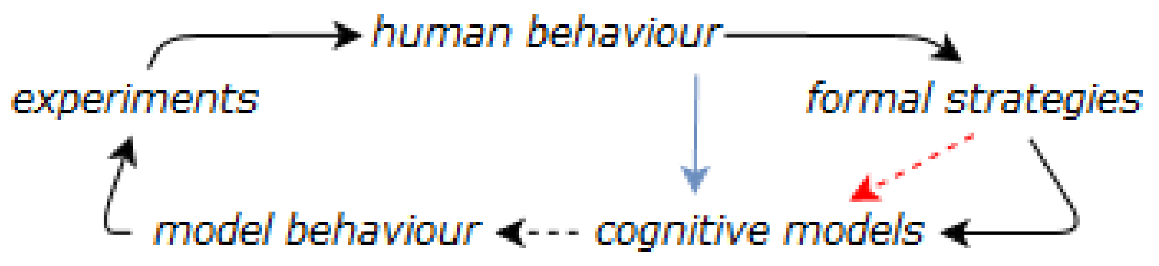
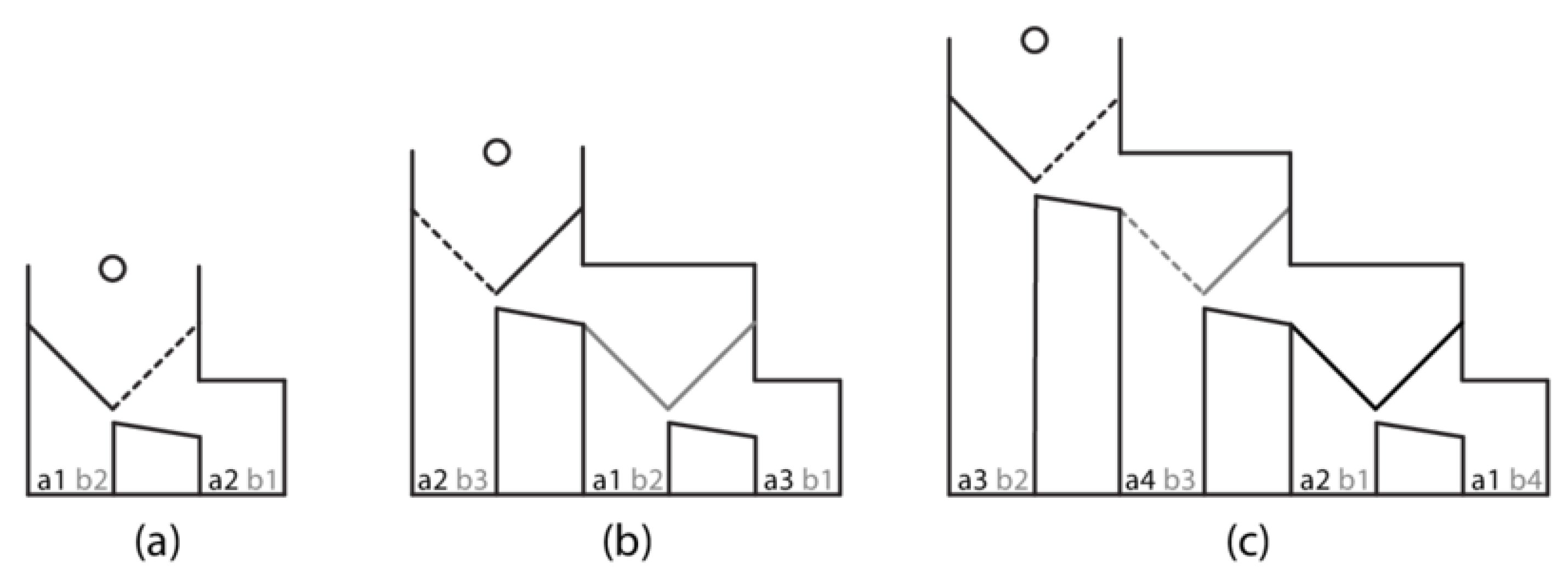
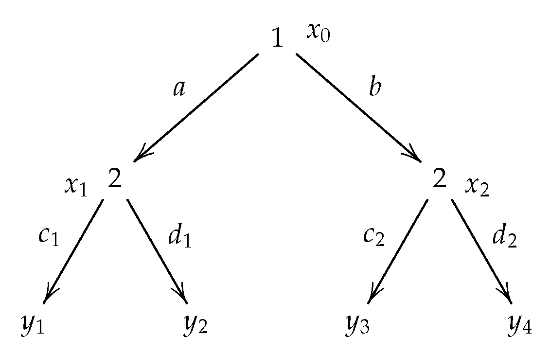
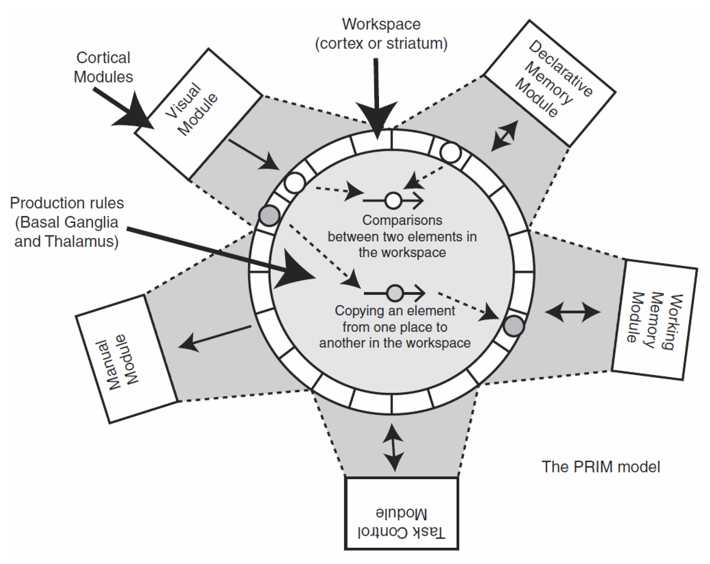
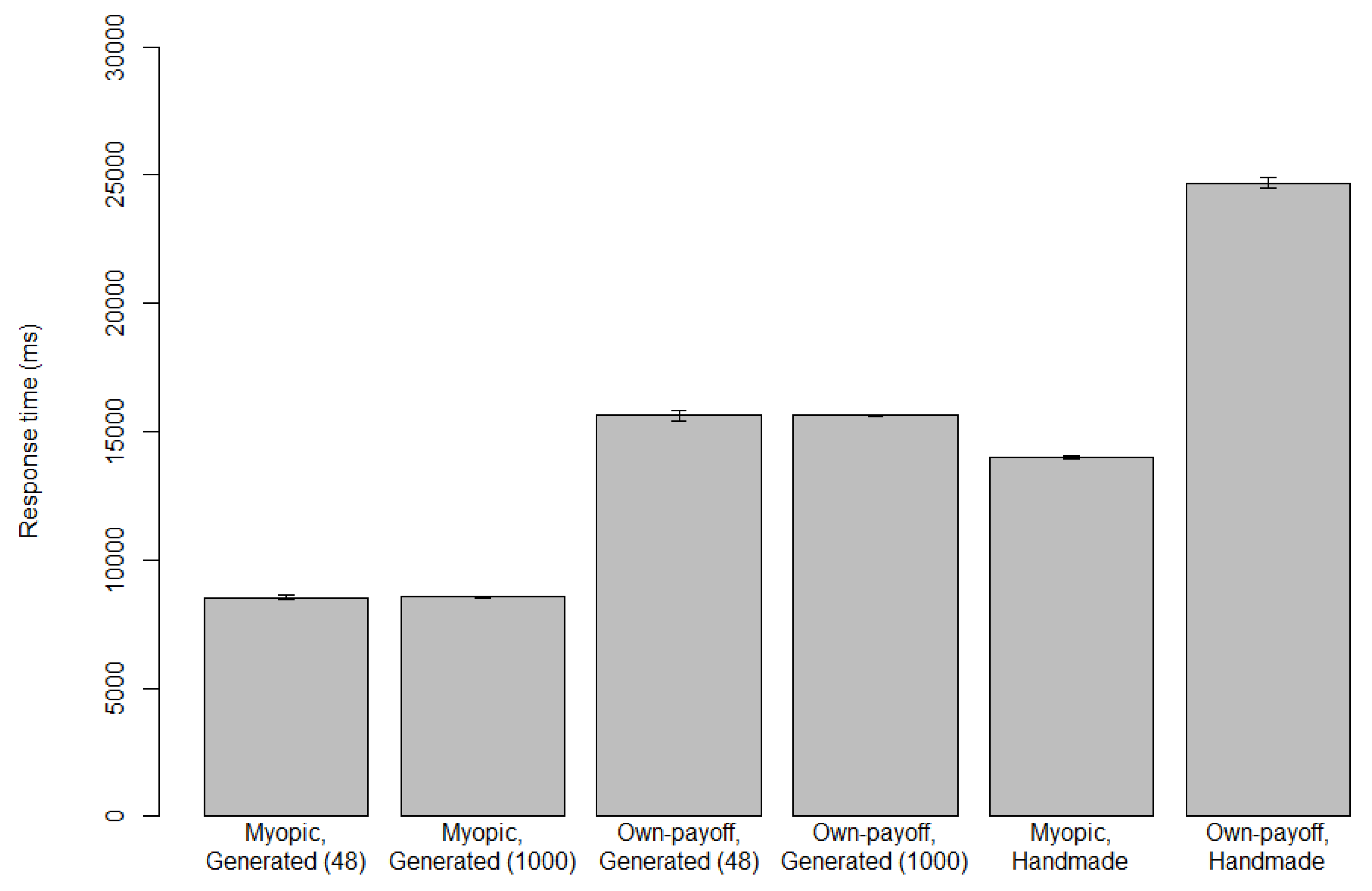
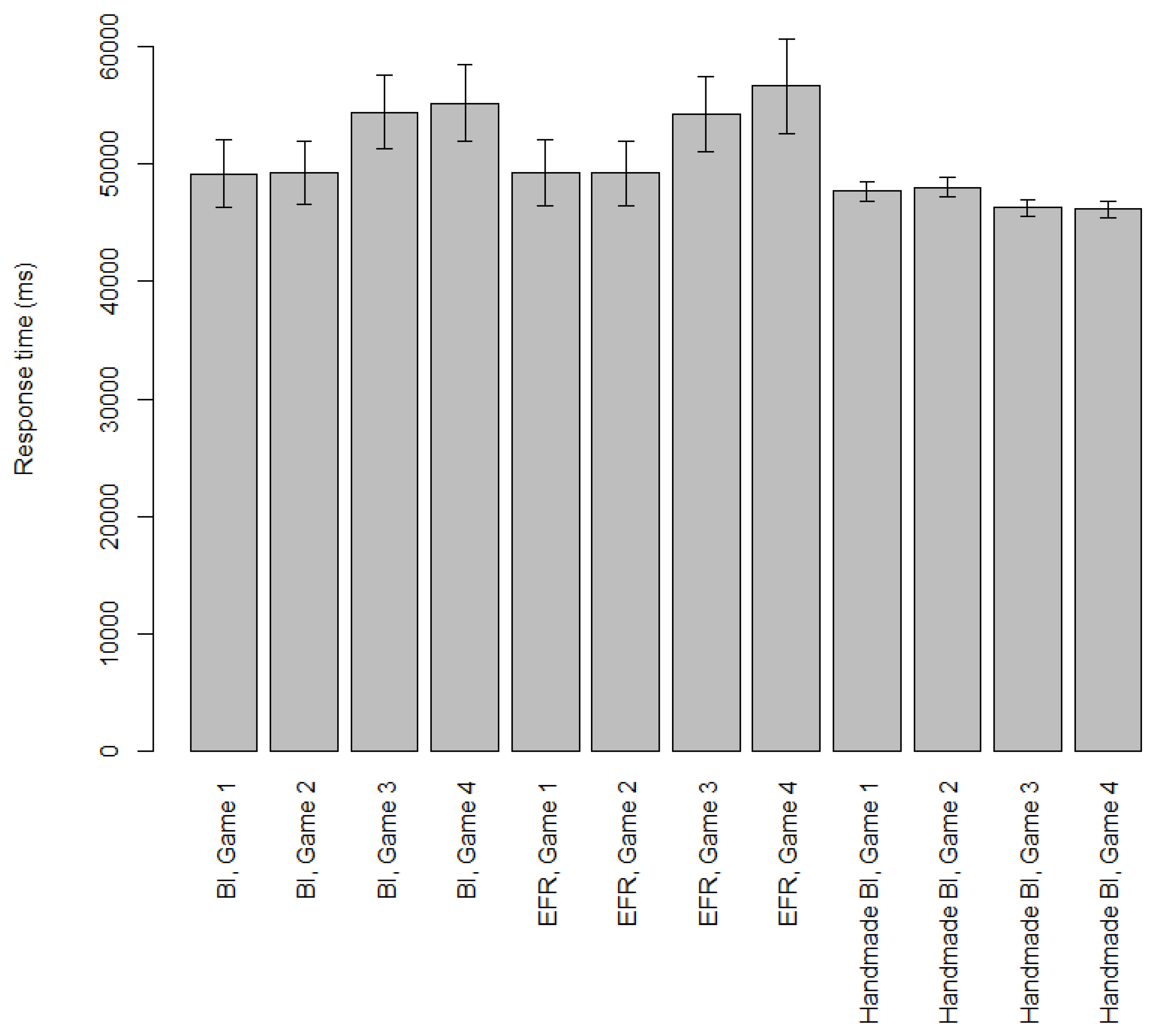
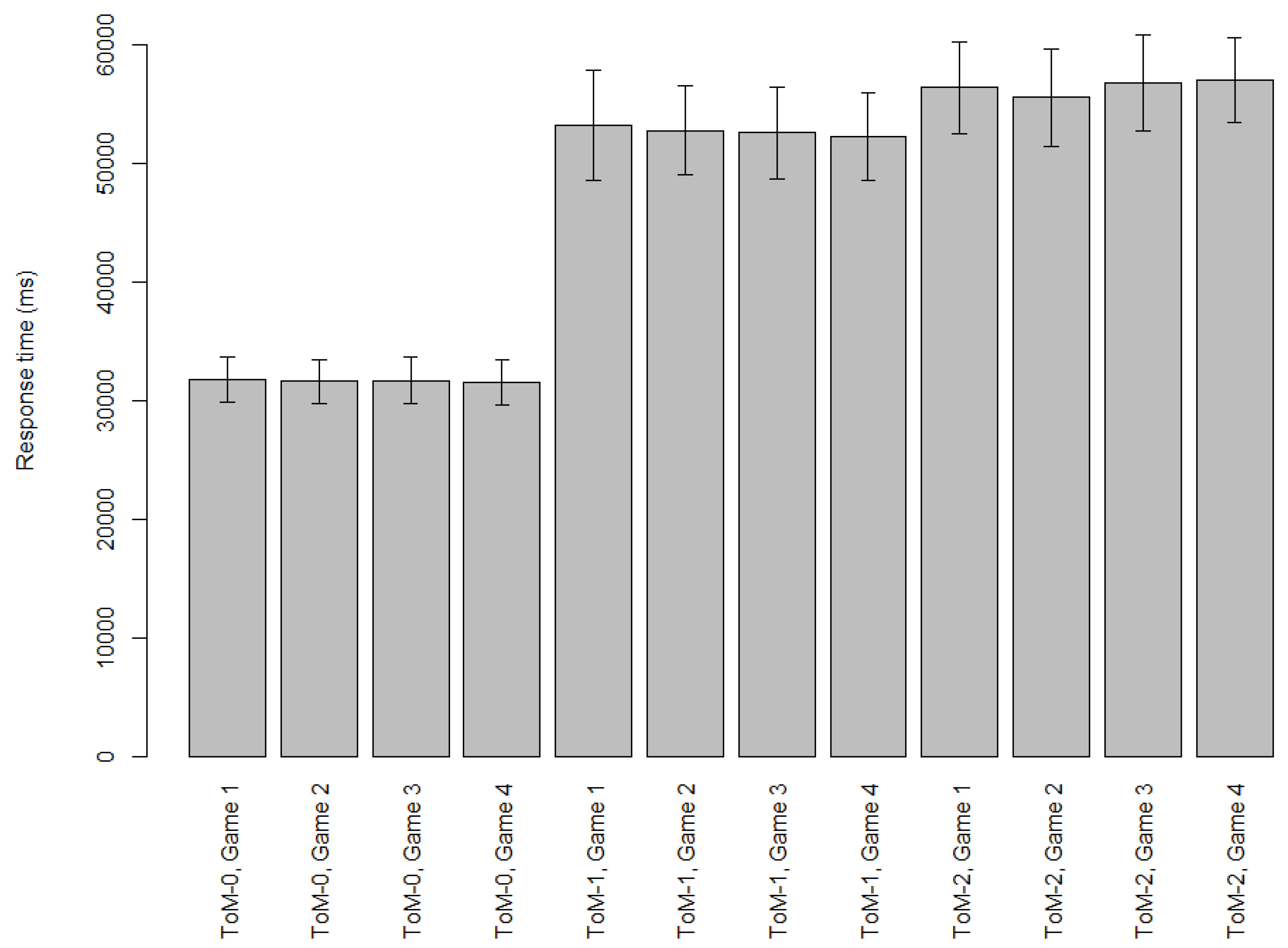
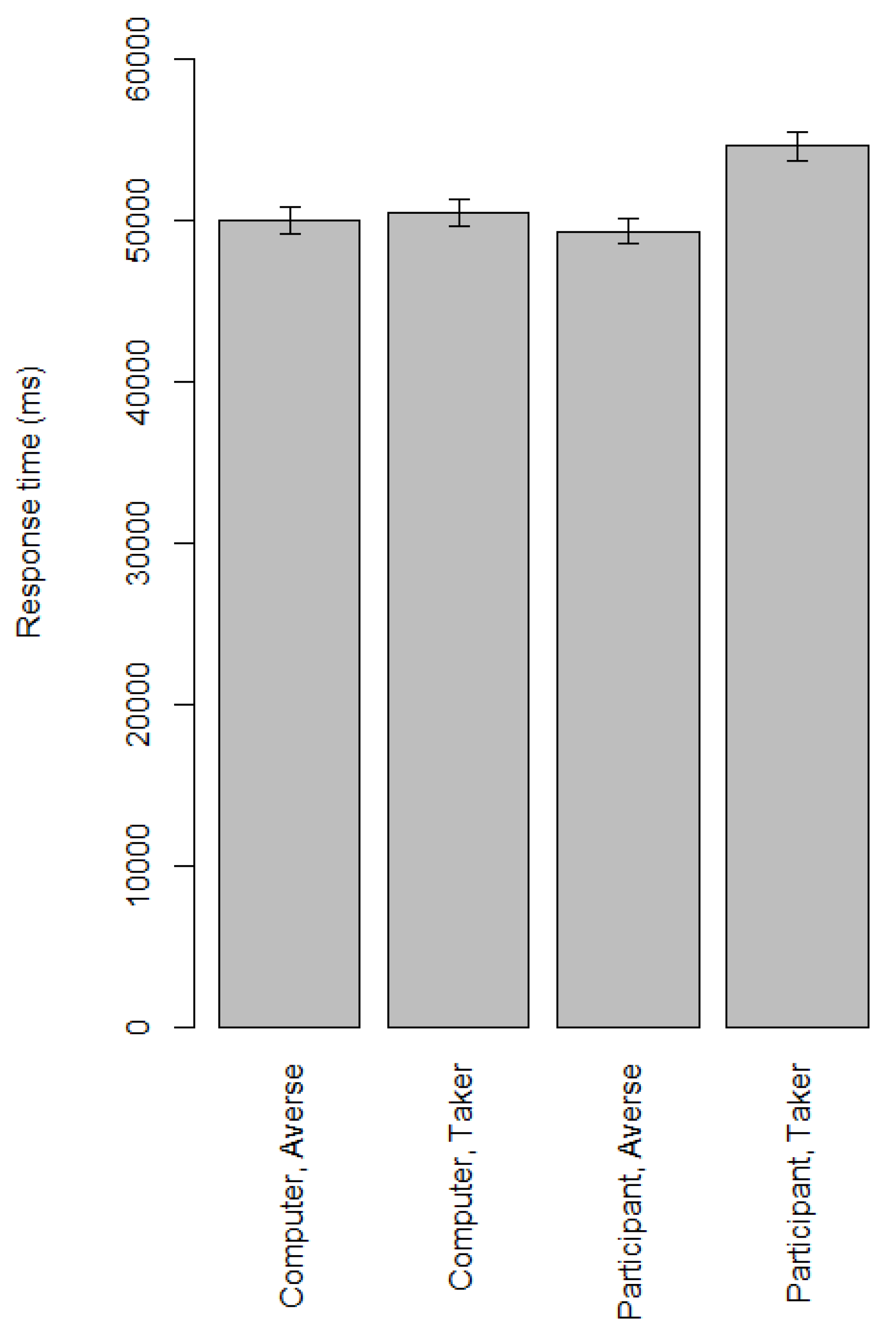
Table 1.
BI, EFR and own-payoff strategies for both players in Games 1–4. For example, P’s EFR strategy d; g in Game 1 stands for: “if the game were to get to P’s first decision point, go right (d); if it were to get to P’s second decision point, go down (g)”.
Table 1.
BI, EFR and own-payoff strategies for both players in Games 1–4. For example, P’s EFR strategy d; g in Game 1 stands for: “if the game were to get to P’s first decision point, go right (d); if it were to get to P’s second decision point, go down (g)”.
| BI Strategies | EFR Strategies | Own-Payoff Strategies | |
|---|---|---|---|
| Game 1 | C: a;e, a;f P: c;g, c;h | C: a;e, a;f P: d;g | C: b;f P: d;g |
| Game 2 | C: a;e, a;f P: c;g, c;h | C: a;e, a;f P: c;g, c;h | C: b;f P: d;g |
| Game 3 | C: a;e, a;f, b;f P: c;g, c;h, d;g, d;h | C: a;e, a;f, b;f P: d;g, d;h | C: b;f P: d;g, d;h |
| Game 4 | C: a;e, a;f, b;e, b;f P: c;g, c;h, d;g, d;h | C: a;e, a;f, b;e, b;f P: c;g, c;h, d;g, d;h | C: b;f P: d;g, d;h |
Table 2.
Proportions c played for myopic and own-payoff cognitive models in Game 5.
| Myopic | Own-Payoff | |
|---|---|---|
| Handmade | 1 | 0 |
| Generated (48 virtual participants) | 1 | 0 |
| Generated (1000 virtual participants) | 1 | 0 |
Table 3.
Proportions c played for BI and EFR in Games 1–4.
| BI | EFR | Handmade BI | |
|---|---|---|---|
| Game 1 | 0.542 | 0.417 | 1 |
| Game 2 | 0.438 | 0.604 | 1 |
| Game 3 | 0.409 | 0.109 | 0.488 |
| Game 4 | 0.543 | 0.596 | 0.503 |
Table 4.
Proportions c played for our risk-based cognitive models in Game 4.
| Risk-Averse, P | Risk-Taker, P | Risk-Averse, C | Risk-Taker, C |
|---|---|---|---|
| 0.7 | 0.163 | 0.581 | 0.338 |
© 2018 by the authors. Licensee MDPI, Basel, Switzerland. This article is an open access article distributed under the terms and conditions of the Creative Commons Attribution (CC BY) license (http://creativecommons.org/licenses/by/4.0/).
Share and Cite
MDPI and ACS Style
Top, J.D.; Verbrugge, R.; Ghosh, S. An Automated Method for Building Cognitive Models for Turn-Based Games from a Strategy Logic. Games 2018, 9, 44. https://0-doi-org.brum.beds.ac.uk/10.3390/g9030044
AMA Style
Top JD, Verbrugge R, Ghosh S. An Automated Method for Building Cognitive Models for Turn-Based Games from a Strategy Logic. Games. 2018; 9(3):44. https://0-doi-org.brum.beds.ac.uk/10.3390/g9030044
Chicago/Turabian StyleTop, Jakob Dirk, Rineke Verbrugge, and Sujata Ghosh. 2018. "An Automated Method for Building Cognitive Models for Turn-Based Games from a Strategy Logic" Games 9, no. 3: 44. https://0-doi-org.brum.beds.ac.uk/10.3390/g9030044
Note that from the first issue of 2016, this journal uses article numbers instead of page numbers. See further details here.