Evolution of Groupwise Cooperation: Generosity, Paradoxical Behavior, and Non-Linear Payoff Functions

1
Department of Biological Sciences, The University of Tokyo, Hongo 7-3-1, Bunkyo-ku, Tokyo 113-0033, Japan
2
Division of Natural Resource Economics, Graduate School of Agriculture, Kyoto University, Oiwake-cho, Kitashirakawa, Sakyo-ku, Kyoto 606-8502, Japan
3
Key Lab of Animal Ecology and Conservation Biology, Institute of Zoology, Chinese Academy of Science, Datun Road, Chaoyang, Beijing 100101, China
4
School of Economics and Management, Kochi University of Technology, Kochi 780-8515, Japan
5
Meiji Institute for Advanced Study of Mathematical Sciences, Meiji Univeristy, Nakano 4-21-1, Nakano-ku, Tokyo 164-8525, Japan
*
Author to whom correspondence should be addressed.
Games 2018, 9(4), 100; https://0-doi-org.brum.beds.ac.uk/10.3390/g9040100
Submission received: 29 September 2018
/
Revised: 8 November 2018
/
Accepted: 13 November 2018
/
Published: 10 December 2018
(This article belongs to the Special Issue The Evolution of Cooperation in Game Theory and Social Simulation)
Abstract
:Evolution of cooperation by reciprocity has been studied using two-player and n-player repeated prisoner’s dilemma games. An interesting feature specific to the n-player case is that players can vary in generosity, or how many defections they tolerate in a given round of a repeated game. Reciprocators are quicker to detect defectors to withdraw further cooperation when less generous, and better at maintaining a long-term cooperation in the presence of rare defectors when more generous. A previous analysis on a stochastic evolutionary model of the n-player repeated prisoner’s dilemma has shown that the fixation probability of a single reciprocator in a population of defectors can be maximized for a moderate level of generosity. However, the analysis is limited in that it considers only tit-for-tat-type reciprocators within the conventional linear payoff assumption. Here we extend the previous study by removing these limitations and show that, if the games are repeated sufficiently many times, considering non-tit-for-tat type strategies does not alter the previous results, while the introduction of non-linear payoffs sometimes does. In particular, under certain conditions, the fixation probability is maximized for a “paradoxical” strategy, which cooperates in the presence of fewer cooperating opponents than in other situations in which it defects.
1. Introduction
Reciprocity is a key factor in the study of evolution of cooperation [1,2]. Evolution of pairwise and groupwise cooperation by reciprocity has been studied by using the two-player and -player repeated prisoner’s dilemma (PD) games [2,3,4,5,6,7,8,9,10,11,12]. While a population of reciprocators can be stable against invasion by defectors in repeated PDs, so long as games are repeated sufficiently many times, various additional mechanisms have been proposed to explain the initial emergence of reciprocators in a population of defectors, such as invasion by a mass of reciprocators [13], formation of spatial clusters [14,15], stochastic aggregate payoffs [16], and random drift [17]. Of particular relevance to the present study is Nowak et al. (2004). They developed a model of stochastic evolutionary dynamics for the two-player repeated PD and derived the fixation probability with which a single mutant of reciprocator that appears in a population of defectors will eventually replace the whole population. Nowak et al.’s (2004) framework has been extended to include the more general -player repeated PD [18,19], which has enabled to investigate the evolution of group-wise cooperation [20,21,22] considering the effect of random drift. In this article, we report our further investigation on the stochastic evolutionary model of the -player repeated PD.
An interesting feature of group-wise cooperation, or more specifically, the -player repeated PD, is that we can conceive of multiple types of reciprocators that differ in their levels of generosity. Take tit-for-tat (TFT) for example. TFT is a reciprocal strategy in the two-player repeated PD, which cooperates in the first round of a repeated game and, from the second round onward, cooperates if and only if its opponent has cooperated in the previous round. In the -player repeated PD, different reciprocal strategies analogous to TFT, or TFTa for , are possible, where represents the strategy’s level of generosity [23]. Namely, TFTa, cooperates in the first round and after that cooperates if and only if or more of its opponents have cooperated in the previous round. Thus, TFTa with a smaller value of is more generous toward the group members’ defection.
Suppose that a single mutant of the strategy that always defects (ALLD) appears in a population of TFTa. Obviously, less generous TFTa (i.e., having larger ) is quicker to find ALLDs in the group and withdraw further cooperation and, thus, more likely to be stable against their invasion. On the other hand, for TFTa to be advantageous over ALLD, it is always necessary that each TFTa individual tends to have or more other TFTa individuals in the same group; otherwise, TFTa cooperates only in the first round of each game to be exploited by ALLDs. This means that more generous TFTa (i.e., having smaller ) may compete better against ALLD, particularly when TFTa is rare in the population; in other words, generosity may serve to facilitate the initial emergence of TFTa.
This intuition has been confirmed by Kurokawa et al. (2010), who compared the fixation probabilities of TFTas with different values of when appears as a single mutant in a population of ALLD [19]. They found that more generous TFTa can sometimes have a greater fixation probability than less generous ones. They also specified the optimal level of generosity that maximizes the fixation probability, showing that there is a certain threshold level of generosity above which the largest fixation probability can never be attained. Specifically, it was shown that any such TFTa that tolerates defections by a half or more of its opponents can never have the largest fixation probability.
Although Kurokawa et al. (2010) focused on the strategies classified as TFTa, they are not the only ones that can potentially establish mutual cooperation in the -player repeated PD. In fact, tolerating the presence of some defectors in a group may have a similar enhancing effect on the evolution of reciprocal strategies in general. However, this possibility has not been explored thus far. Here we extend Kurokawa et al.’s (2010) analysis to consider the set of all “reactive strategies” that (i) cooperates with probability in the first round and (ii) cooperates in the th round () with probability , which depends on the number of opponents, , who have cooperated in the th round. There are such strategies in total, including TFTas and strategies that defect in the first move [24,25,26,27,28]. The rest of the strategies in the set are “paradoxical” in the sense that each of them has a certain situation in which it cooperates even though there are fewer cooperators in the group than in other situations in which it withdraws cooperation. It is of interest whether the strategies defecting in the first move or exhibiting paradoxical behavior can have the largest fixation probability among the set of all reactive strategies when invading ALLD.
Another limitation of Kurokawa et al.’s (2010) work is that they only considered the conventional linear payoff functions (i.e., linear public goods games. However, there are at least two reasons why non-linear payoff functions should be also considered. First, in the real world, payoffs are not always linear [29,30,31,32,33,34,35,36,37,38,39] and it has been demonstrated that introduction of non-linearity can affect the outcome of evolutionary models (e.g., [40,41,42,43,44,45,46,47]. Second, if payoffs increase non-linearly with the number of cooperating members in the group, it can be said that the efficiency of an act of cooperation varies depending on the number of cooperators. For example, in case payoffs increase more rapidly when cooperators are fewer, an individual’s act of cooperation is more efficient in the presence of fewer cooperators. In such a case, more generous strategies may be selectively favored because generosity promotes cooperation when it is efficient. To examine these possibilities, we also extend Kurokawa et al. (2010) in terms of payoff functions.
In addition, Kurokawa et al. (2010) derived their results under the assumption that selection is sufficiently weak. However, the intensity of selection can affect the outcomes of evolutionary models (e.g., [17,48,49,50]. Hence, we investigate to what extent our results based on the weak selection assumption may be affected by the selection intensity.
In this paper, we extend Kurokawa et al.’s (2010) analysis by removing these limitations. In particular, taking non-linear payoff functions and paradoxical (i.e., non-tit-for-tat type) strategies into consideration, we ask how non-linear payoffs may facilitate the evolution of excessive generosity and whether any paradoxical strategies can ever attain the highest fixation probability among all reactive strategies considered. Additionally, we examine how our results may depend on the intensity of natural selection. In what follows, we first introduce the -player repeated PD and our model of stochastic evolutionary dynamics (Model). Then we derive, based on the weak selection approximation, the best reactive strategies, or the strategies maximizing the fixation probability, and provide detailed analyses for linear and non-linear payoff cases. We also examine to what extent our results may be affected if selection is not sufficiently weak (Results). Finally, we summarize the results and discuss some caveats and possibilities of further investigations (Discussion).
2. Model
We investigate stochastic evolutionary dynamics of a population of individuals whose fitness is determined by -player repeated PD games. We consider a set of “reactive strategies,” as defined below, and compare the fixation probabilities of different reactive strategies when introduced as a mutant into a population of the strategy that always defects, or ALLD. Our goal is to specify the “best reactive strategies,” which maximize the fixation probability.
2.1. The -Player Repeated Prisoner’s Dilemma
In the n-player repeated PD, a group of individuals play a game consisting of one or more rounds, in each of which each individual chooses to either cooperate or defect. After one round is finished, another round will be played with probability ; otherwise, the group will be dismissed (. Thus, the expected number of rounds is . Suppose that there are cooperating and defecting individuals in a given round. The payoffs to cooperating (C) and defecting (D) individuals in that round are denoted by and , respectively (. Note that and are defined arbitrarily and used only for the sake of notational convenience. Following Boyd & Richerson (1988), n-player PD requires the following four conditions to be satisfied:
where . Conditions (1) states that an individual always gains more from defecting than cooperating. Conditions (2) and (3) mean that an individual always gains more when there are more cooperators in the group. Conditions (4) indicates that the total payoff of the group is larger when there are more cooperators in the group.
We define a reactive strategy in the -player repeated PD as follows: an individual with a reactive strategy cooperates with a certain probability in the first round, and from the second round on, cooperates with a certain probability determined by the number of opponents (i.e., group members other than the self) who have cooperated in the preceding round. Any reactive strategy is described by a vector , where denotes the probability with which an individual obeying this strategy cooperates in the first move and denotes the probability with which he cooperates in a given round, provided that of the opponents have cooperated in the preceding round. We focus on the set, , of all reactive strategies in which is either 0 or 1 and is either 0 or 1, namely, . Obviously, there are strategies in .
Table 1 shows the payoff matrix of the general two-strategy -player game, where denotes the payoff to an individual with strategy A whose opponents are individuals with strategy A and individuals with strategy B; likewise, denotes the payoff to an individual with strategy B confronting with the same composition of opponents. Let A and B in Table 1 represent a strategy in and ALLD, respectively. To describe the game involving and ALLD, we need to write down all and in Table 1 in terms of , , , and . Consider a group consisting of individuals adopting and individuals adopting ALLD. We denote by the expected number of rounds in which a individual cooperates before the group is dismissed. Since there are on average rounds, we have Further, since we do not consider any errors in behavior, individuals perfectly coordinate their behavior, that is, either all or none of them cooperate in a given round. Hence, we obtain:
For any group composition, is determined by , , and in the following manner. First, suppose that . In this case, never defects and, hence, . Second, if and , cooperates only in the first round and, thus, . Third, if and , alternates cooperation and defection indefinitely, in which case . Fourth, if , defects in every round and hence . Fifth, if and , defects only in the first round and thus Sixth, if and , alternates defection and cooperation indefinitely, in which case . In sum, is given by:
Therefore, an -player repeated PD involving and ALLD is specified using Equations (5)–(7).
2.2. Evolutionary Dynamics
We use a model of stochastic evolutionary dynamics developed for the general two-strategy -player game [18]. A population consisting of individuals adopting strategy A and individuals adopting strategy B is considered, where the population size, , is constant (. Groups of individuals are formed by choosing individuals at random from the population and a game is played within each of these groups (. The payoffs of the game are as shown in Table 1. Let and be the expected payoffs to an A individual and a B individual, respectively, when the number of A individuals in the population is . The fitness of A and B individuals are given by and , respectively, where is the selection intensity (. The population dynamics are formulated as a Moran process with frequency-dependent fitness: at each time step, an individual is chosen for reproduction with the probability proportional to its fitness, and then one identical offspring is produced to replace another individual randomly chosen for death with probability 1/N [17,51]. Denote by the probability that a single individual with strategy A in a population of N − 1 individuals with strategy B will finally take over the whole population (i.e., the fixation probability). Throughout the paper, we assume that the interaction group is smaller than the population (. Here, we have:
where represents a binomial coefficient when and is defined zero when .
3. Results
3.1. General Case
We define the best reactive strategy as the strategy (or strategies) that maximizes the fixation probability when introduced as a single mutant in a population of ALLD. The best reactive strategy maximizes the right-hand side of Equation (10) in the context of the -player repeated PD specified by Equations (5)–(7). Equation (10) is equivalent to:
Putting Equations (5) and (6) into Equation (11) and explicitly denoting the dependence on strategy , we obtain:
where:
is independent of strategy . Note that is given by Equation (7) and is dependent on in the following manner:
The best reactive strategy is given by the following equation:
As shown in Appendix A, the solution of the maximization problem in Equation (15) is given as follows. On the one hand, when:
the solution of Equation (15) is given by:
for . Note that can be either or in case . On the other hand, when the inequality in Inequality (16) is reversed, the solution of Equation (15) is given by:
where can be either or for . In sum, Conditions (16)–(18) specify the best reactive strategy, .
Our main result Conditions (16)–(18) states that so long as the game is repeated sufficiently many times (i.e., is sufficiently large), each bit, , of the best reactive strategy is solely determined by the sign of , which is determined by the payoff structure of the game (and the group size and the population size. In Equation (13), the term is the payoff to a cooperating player in a group where k players cooperate minus the payoff to a defecting player in a group where no one cooperates. Thus, this term represents the benefit of cooperation. The term represents the payoff difference between a cooperating player and a defecting player in a group where k individuals cooperate. Thus, this negative term represents the cost of cooperation. Weighted sum of them determines whether the best reactive strategy should cooperate if players have cooperated in the previous round.
In the following analysis, we consider cases in which Inequality (16) holds unless otherwise stated.
3.2. Linear Payoff
Let us begin with a special case where the following conventional linear payoff assumption holds:
From Inequalities (1)–(4), it has to be that . Putting Equations (19) and (20) into Equation (13), we obtain:
Since increases linearly with in this case, there exists a critical value above which is positive (Figure 1a. Hence, from Equation (17), is maximized when the following condition is met:
where:
From Equation (23), decreases with increasing , and for an infinitely large population, is given by:
Since by assumption, holds. Therefore, any strategy that cooperates when a half or less of the opponents have cooperated in the previous round cannot be the best reactive strategy.
A similar, but slightly different, result has been obtained by Kurokawa et al. (2010) [19]. They examined the fixation probability of a strategy called TFTa, being introduced as a mutant into a population of ALLD, under the linear payoff assumption as given by Equations (19) and (20). An individual adopting TFTa cooperates in the first round, and from the second round on, cooperates if and only if or more of the opponents have cooperated in the previous round, where measures the level of generosity [23]. Thus, there are strategies that are classified as TFTa with different levels of generosity. From these, Kurokawa et al. (2010) specified , the optimal level of generosity, which maximizes the fixation probability. In the terminology of the present study, the strategies constitute the subset of for which and . In addition to these, we consider two kinds of non-TFTa reactive strategies. One is those that defect in the first round (i.e., . Our analysis shows that some of this kind can maximize the fixation probability if the expected number of rounds is sufficiently small, partially modifying Kurokawa et al.’s (2010) finding. Another kind is what we call “paradoxical” strategies (see Introduction), in which holds for at least some ; for example, . It turns out that Equations (22)–(24) is equivalent to the optimal level of generosity obtained by Kurokawa et al. (2010). Thus, their result is not changed by taking paradoxical strategies into consideration.
3.3. Non-Linear Payoff
The n-player PD can be further subcategorized according to characteristics of the fitness functions [39,46]. To illustrate, we define the cost and benefit associated with cooperation as:
respectively. From Inequalities (1) and (2), is required for all . We can measure how the cost and benefit depend on the number of cooperators by considering:
For example, when holds for all , the cost is constant. Let us also consider:
for . It should be intuitively clear that the n-player PD requires , which is equivalent to (3), while can be either positive or negative (or zero. If, for instance, holds for all , the benefit increases in an accelerative manner with the number of cooperators (e.g., the weakest-link game; [56]), whereas if always holds, the increase is decelerated (e.g., the volunteer’s dilemma; [57]. The class of n-player PDs for which always holds represent the public goods games in which the amount of public goods increases linearly with the number of cooperators [47].
The linear payoff assumptions in Equations (19) and (20) mean that the following conditions are satisfied for all :
Below we examine how evolution of generosity and paradoxical behavior may be affected by relaxing Equations (30) and (31).
3.3.1. Evolution of Generosity with Non-Linear Payoff
Constant Cost with Non-Linear Benefit
Consider the case when there is no restriction on the benefit function (except Inequalities (1)–(4)), that is, Equation (30) is not necessarily true. For the moment, we assume Equation (31). From Equations (13) and (20), we have:
Using Conditions (1) and (20), we obtain:
which gives:
Thus, we obtain a necessary condition for , namely:
The right-hand side of Inequality (35) decreases and approaches with increasing . Hence, from Equation (17), holds in the best reactive strategy only if . This means that any strategy who cooperates when a half or less of the opponents have cooperated in the previous round cannot be the best reactive strategy.
Variable Cost with Non-Decelerating Benefit
Let us now remove the restriction on the cost function, that is, we consider the case when Equation (31) does not necessarily hold. Instead of Equation (30), we assume:
which means that the benefit from cooperation increases with the number of cooperators in either linear or accelerative fashion. From Equations (13), (26) and (28), we have:
Using Inequality (36), we obtain:
From Conditions (37) and (38), we have:
Meanwhile, using Conditions (1), (25), (26) and (28), we obtain:
Therefore, combining Equation (39) and (40), we obtain:
Hence, as in the case of constant cost, Inequality (35) is necessary for , which again means that the best reactive strategy must defect when a half or more of the opponents have defected in the previous round.
A Numerical Example
The results for the above two special cases are consistent with our finding in the analysis under the linear payoff assumption. However, the result may be altered qualitatively in the absence of any restriction on the benefit or cost functions. As an illustration, consider the following payoff functions:
which satisfies Inequalities (1)–(4), but is not consistent with Equations (30) or (31). To be specific, let us set , , and . Putting them into Equation (13), we obtain:
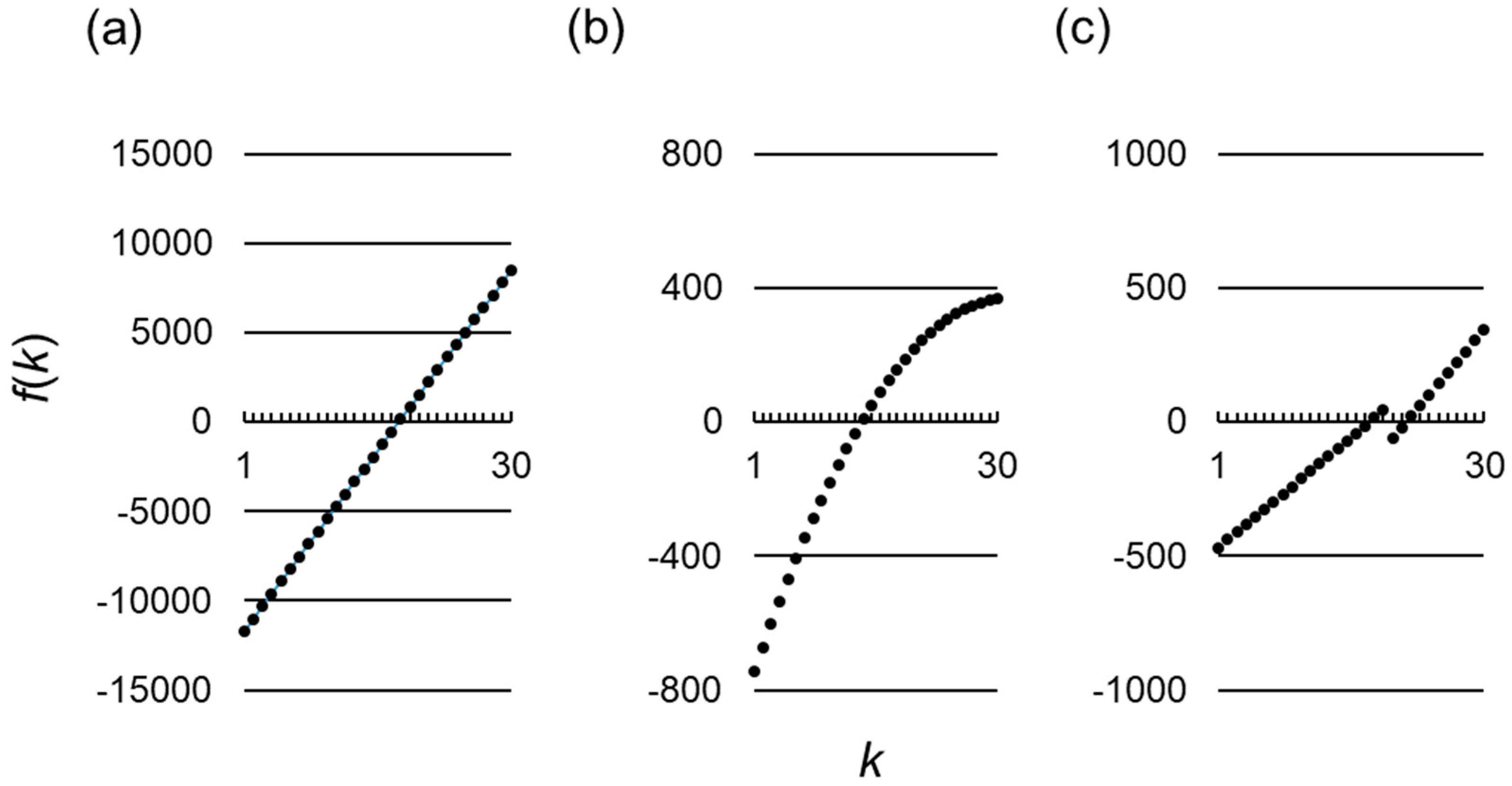
In this case, Inequality (16) is met, and as shown in Figure 1b, holds if and only if . Hence, from Equation (17), the best reactive strategy () satisfies the following:
Remember that is defined as the probability with which he cooperates in a given round, provided that of the “opponents” have cooperated in the preceding round. This demonstrates that there exist situations in which such a strategy that cooperates when a half or more of the opponents have defected in the previous round can be the best reactive strategy.
For comparison, the second and third best strategies following Equation (45) are given by:
respectively. For , the approximated fixation probabilities for Equations (45)–(47), calculated from Equation (9), are 0.00254215, 0.00254207, and 0.00254176, respectively.
3.3.2. Evolution of Paradoxical Behavior with Non-Linear Payoff
Non-Increasing Cost and Non-Linear Benefit
Consider the case when there is no restriction on the benefit function (except Inequalities (1)–(4)) and, thus, Equation (30) is not necessarily true. As for the cost function, we partially relax Equation (31) by assuming instead:
which means that the cost of cooperation either is constant or decreases with increasing number of cooperators. Equation (13) changes into:
Hence, we have:
From Conditions (48)–(50), we have:
This means that if then for any . Hence, from Equation (17), a paradoxical strategy cannot be the best reactive strategy.
A Numerical Example
Our analysis thus far has shown that a paradoxical strategy cannot be the best reactive strategy so long as the cost of cooperation is either unaltered or decreased by increasing number of cooperators. However, this may not be the case if the cost of cooperation sometimes increases with the number of cooperators. Let us provide a numerical example in which the best reactive strategy exhibits a paradoxical behavior. We set , , , and and assume that Equation (30) is met. Instead of Equation (31), here we assume:
for which Inequalities (1)–(4) are satisfied. This represents a case when the cost of cooperation is larger in the presence of more cooperators in the group. Intuitively, in such a situation, a paradoxical strategy that cooperates only when there are relatively few cooperators may be more advantageous than non-paradoxical strategies that, which cooperate whenever the number of cooperators exceeds a threshold. Indeed, since in this case Inequality (16) is met, and is non-monotonic in this case (Figure 1c), the best reactive strategy () is given from Equation (17) by:
That is, the best reactive strategy cooperates when there are 17 or more opponents who have cooperated in the previous round, except when the number of cooperators is 19 or 20, in which case it defects. The relative advantages of cooperation and defection are determined by a balance between the following two factors: On the one hand, obviously, cooperation is more advantageous when the associated cost is smaller. On the other hand, given that the cost is constant, the relative advantage of cooperation increases with the number of cooperators in the group. In the current example, there is a rise of the cost at (see Equation (52)), which can be compensated for only when the number of cooperating opponents increases to 21 or more.
The second and third best strategies following Equation (53) are given respectively by:
For , the fixation probabilities of strategies Equations (53)–(55) with the small approximation are 0.00251170, 0.00251155, and 0.00251154, respectively.
3.4. The Best Reactive Strategy under Moderate Selection Intensity
Thus far we have assumed that selection is sufficiently weak () so that the fixation probabilities can be approximated by Equation (9). Here we numerically obtain the exact fixation probabilities using (8) without the weak selection assumption to examine how this may affect the identity of the best reactive strategy.
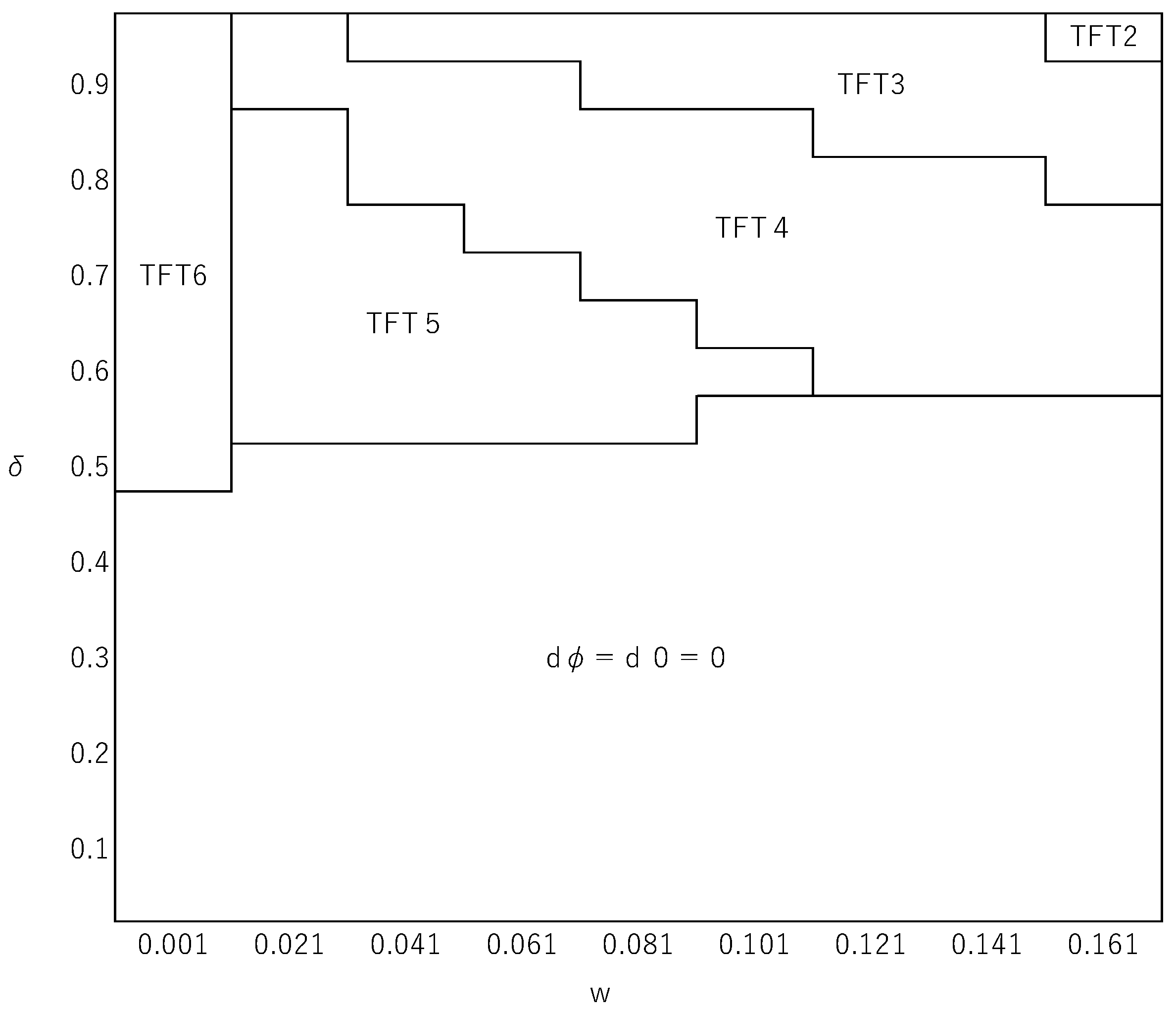
For simplicity, we make the linear payoff assumption, Equations (19) and (20). Figure 2 illustrates how the best reactive strategy (), obtained by using Equation (8), changes depending on the values of and for parameter values , , , and . For this parameter setting, a comparison of fixation probabilities calculated from Equation (9) would indicate TFT6 as the best reactive strategy when holds, where , and when . This gives a good approximation of the exact numerical solution for as shown in Figure 2. However, when is larger, the approximation is no longer valid. Figure 2 shows that there exist situations in which such a strategy that cooperates when a half or more of the opponents have defected in the previous round can be the best reactive strategy, which cannot be the case in the limit of week selection. A reactive strategy’s fixation probability is determined by its payoffs relative to the unconditional defector at various frequencies ( in Equation (8). Among the values, a relative payoff at a lower frequency has a greater impact on the fixation probability. Hence, if, as numerically suggested by Kurokawa et al. (2010), the relative payoff at a low frequency tends to be larger for more generous reactive strategies, this is likely to favor the evolution of generosity. This effect might be more pronounced when selection, rather than random drift, plays a greater role. These considerations all in all accord with our numerical example suggesting that more generous reactive strategies are selectively favored when selection is more intense. It was also numerically shown that can affect the identity of the best reactive strategy, while in the limit of weak selection does not affect what the best reactive strategy is as far as it satisfies Inequality (16). In addition, within this particular range of parameter values, we did not find any case in which a paradoxical strategy is the best reactive strategy.
4. Discussion
We have investigated stochastic evolutionary dynamics of a population in which an individual’s fitness is determined by the n-player repeated PD. We have compared the fixation probabilities of different reactive strategies when they appear as a rare mutant in a population of unconditional defectors. Reactive strategies in our analysis are described by a vector , where represents the probability with which the strategy cooperates in the first round and represents the probability with which the strategy cooperates in a given round of a repeated game when of the opponents have cooperated in the previous round. We have considered a set, , of all reactive strategies for which is either 0 or 1 and is either 0 or 1 to specify the best reactive strategy attaining the maximum fixation probability. In a repeated PD, after one round is played, another round will be played with probability . Under the assumption of weak selection, we have specified a threshold of below which all strategies satisfying are the best reactive strategies. We have also found that when exceeds the threshold, of the best reactive strategy is solely determined by the sign of , as given by Equation (13), which is interpreted as a weighted sum of the cost and benefit of cooperation when opponents have cooperated in the proceeding round.
The present study extends our previous analysis (Kurokawa et al. (2010), [19]) by considering a broader set of reactive strategies and non-linear payoff functions. We also investigate how robust the indicated identity of the best reactive strategy is to deviations from the weak selection assumption. Kurokawa et al. (2010) specified the best reactive strategy from reactive strategies classified as TFTa, which constitute a subset of , under the conventional linear payoff assumption. One of their findings was that any TFTa that tolerates defection by more than a half of the group members can never be the best reactive strategy. The present study has shown, on the one hand, that under the linear payoff assumption, the previous finding holds true even for all reactive strategies in . For non-linear payoff functions, on the other hand, we have shown that the previous finding does not always hold, that is, when the benefit increases in a decelerative manner with the number of cooperators, the best reactive strategy tolerates defection by more than a half of the opponents. We have also found that a strategy tolerating defection by more than a half of the opponents can be the best reactive strategy when selection is not weak.
We have also demonstrated that a paradoxical strategy, in which holds for at least some , can be the best reactive strategy when the cost of cooperation increases with the number of cooperators in a group. As far as we know, it has not been pointed out that a conditional cooperator can sometimes do better by behaving paradoxically in competition with defectors. A potentially relevant observation is that human participants in laboratory experiments of the repeated PD sometimes behave as if they were following a paradoxical strategy (e.g., [58,59,60,61]), though these studies assume linear payoff functions. The present study suggests that it may be of interest to investigate the effect of the shape of the payoff functions on the occurrence of paradoxical behaviors in the laboratory setting.
So far, we have examined the fixation probability of strategy when appeared as a single mutant in a population of ALLD. In Appendix B we also compare the fixation probability of ALLD when introduced as a single mutant in a population of reactive strategy , across all in . A reactive strategy associated with a lower fixation probability of ALLD is regarded as more robust against invasion by ALLD. The reactive strategy that minimizes the fixation probability of ALLD turns out to be TFTn-1, that is, , when is larger than the threshold specified by Inequality (16), and the strategies satisfying when otherwise. Further, we investigate the ratio of the fixation probability of in a population of ALLD to the fixation probability of ALLD in a population of , across all in . As shown in Appendix C, the reactive strategy maximizing the ratio of the fixation probabilities is TFTn-1 when is larger than the threshold, and when otherwise. These results are consistent with our earlier analysis [19], even though the present study considers paradoxical strategies and non-linear payoff functions, which were not considered in the previous study.
Natural selection is regarded as favoring a mutant reactive strategy replacing a population of ALLD if the fixation probability of the reactive strategy exceeds , which is the fixation probability for neutral evolution. The reactive strategies that are the best when is small so that Inequality (16) is not satisfied (i.e., ) always have the fixation probability . Thus, when Inequality (16) is not met, the best reactive strategies and ALLD are selectively neutral. On the other hand, when is large so that Inequality (16) is satisfied, there are other reactive strategies, including the best one, with the fixation probability larger than . Hence, in this case, the best reactive strategy is always selectively favored over ALLD. See Appendix D for a further analysis on the case assuming linear payoff functions.
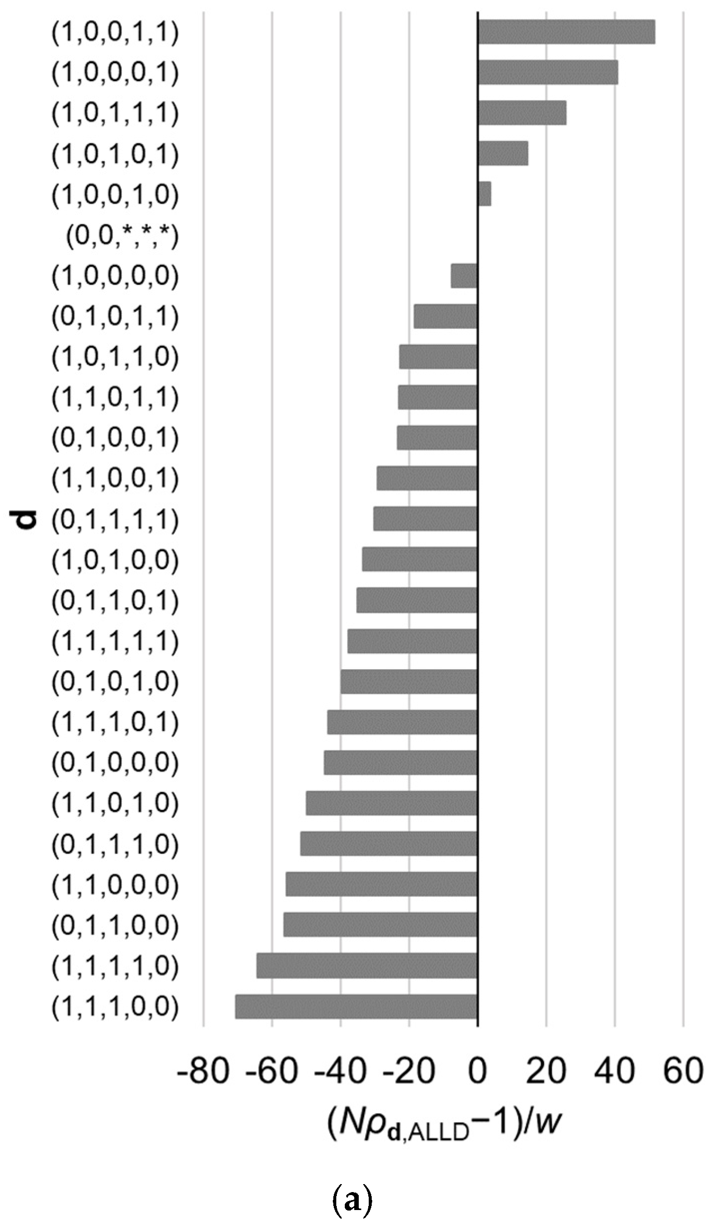
Thus far, our focus has been on the best reactive strategy, which maximizes the fixation probability. However, it is also of interest to examine characteristics of other reactive strategies whose fixation probabilities are relatively high and difference in fixation probabilities among those best strategies. For example, Table 2 gives a list of ten best strategies in the case of assuming Equations (19) and (20). Figure 3 illustrates the fixation probabilities of the 32 possible strategies in the case of for various values of , under the assumption of Equations (19) and (20). The value of makes difference in the order of the strategies. Note that as shown in Appendix A, the value of does not have an effect on the order of the strategies belonging to subset of .
Finally, let us conclude by mentioning two issues to be addressed in future research. First, actual human behavior can be more complex than that in our model. Although the present study considers a greater variety of reactive strategies than in a previous study [19], the strategy set can be further broadened. Our strategy set, , does not include, for example, continuous strategies that engage in partial cooperation (see [62]), or those that make decisions referring to their own past behaviors ([63,64,65,66,67,68]. In addition, in our analysis, the benefit, , and the cost, , of cooperation are assumed to be the same for all individuals. Namely, we assumed that there are no differences among agents in this sense. In reality, however, individuals may have different values of and , and these variations could affect the model outcome [69]. Secondly, we have assumed that perfect information regarding group members’ behaviors is always available. It has been shown, however, that results of related models may be qualitatively altered depending on the accessibility of the relevant information [45,64,70,71,72,73,74,75].
Author Contributions
Every author was involved in all stages of development and writing of the paper.
Funding
S.K. is partially funded by Chinese Academy of Sciences President’s International Fellowship Initiative. Grant No. 2016PB018 and Monbukagakusho grant 16H06412. J.Y.W. is partly supported by JSPS Kakenhi 16K05283 and 16H06412. Y.I. is partly supported by the JSPS aid for Topic-Setting Program to Advance Cutting-Edge Humanities and Social Sciences Research and Kakenhi 16K07510 and 17H06381.
Acknowledgments
We thank Yoshio Kamijo (Kochi University of Technology) for discussions.
Conflicts of Interest
The authors declare no conflict of interest.
Appendix A
Solving (15)
To solve the maximization problem Equation (15), we first consider subsets of reactive strategies satisfying and , where:
we derive the solution, (), within each subset, after which the solution in is obtained by comparing the maxima of within the subsets.
First, when and , Equation (7) gives:
Note that in this case depends only on a single component () of . Since is constant and the right-hand side of Equation (A2) increases with , the solution of the maximization problem within subset is given by:
for . In case , both and are the solutions. Hence, from Equations (12), (A2) and (A3), we obtain the maximum of within as follows:
Note that we use (from Conditions (1), (2) and (13)) in the derivation of Equation (A4).
Second, when , we have:
which increases with . Thus, the solution in this case is given as well by Equation (A3) for . Accordingly, the maximum of within is given by:
Third, when , we have:
This means that all combinations of for are the solutions and the maximum of within is:
Fourth, when and , we obtain:
which increases with . Hence, the solution in this case is also given by Equation (A3) for . Therefore, the maximum of within is given by:
Finally, a comparison of Equations (A4), (A6), (A8) and (A10) shows that the solution of Equation (15) depends on the expected number of rounds, , as shown in Conditions (16)–(18). Note that as Equations (A2), (A5), (A7) and (A9) indicate, does not affect the rank order of reactive strategies in the magnitudes of the fixation probabilities within each subset.
Appendix B
The Fixation Probability of ALLD as a Single Mutant in a Population of d
Under the assumption of weak selection, the fixation probability, , of a single individual with strategy B in a population of individuals with strategy A is given approximately by:
where:
Let us specify the reactive strategy that minimizes the fixation probability of ALLD. Putting Equations (5) and (6) into Equation (B2), we obtain:
where:
is independent of strategy . Since and always hold, we have .
Firstly, when and , Equations (7) and (A13) show:
From Equation (A15), since and always hold, is minimized when , for and . This means that the fixation probability of ALLD is minimized in a population of strategy , namely, TFTn−1 in . In this case, the minimum of is given by:
Secondly, when , (A13) becomes:
Since and , is minimized when , for and . Hence, the minimum of in is given by:
Thirdly, when , Equations (7) and (A13) indicates that always holds. Hence, irrespective of the values of for , the minimum of in is:
and fourthly, when and , Equation (A13) becomes:
Since and , is minimized when , for and . Thus, the minimum of in is:
A comparison of Equations (A16), (A18), (A19) and (A21) shows the following. The strategy that minimizes among all strategies in is TFTn−1 when:
and any strategy satisfying when the inequality in Equation (A22) is reversed. This means that the fixation probability of ALLD is minimized in a population of strategy , namely, TFTn-1 when exceeds a threshold and otherwise, it is minimized in a population of strategies satisfying .
Appendix C
The Ratio of the Fixation Probabilities
Ratio can be viewed as a measure of the selective advantage of A over B for the long-term evolutionary process. From Equations (9) and (A11), the ratio is given approximately by:
where:
We regard A and B as strategy and ALLD, respectively, to specify the reactive strategy that maximizes the ratio of the fixation probabilities. Putting Equations (5) and (6) into Equation (A24) yields:
Firstly, when and , by using Equation (7), Equation (A25) becomes:
Since and always hold, is maximized when , for and . This means that the largest ratio of the fixation probabilities is attained by strategy , namely, TFTn−1. Hence, the maximum of in is given by:
Secondly, when , Equation (A25) becomes:
Since and , is maximized when , for and . Thus, the maximum of in is:
Thirdly, when holds, Equation (7) and Equation (A25) indicate that is always true, irrespective of the values of for . Therefore, the maximum of in is:
Fourthly, when and , by using Equation (7), Equation (A25) becomes:
Since and always hold, is maximized when , for and . Hence, the maximum of in is given by:
Finally, by comparing Equations (A27), (A29), (A30) and (A32), we obtain the following result. Of all strategies in , the strategy maximizing is TFTn−1 when:
and any strategy satisfying when the inequality in Inequality (A33) is reversed. This means that the largest ratio of the fixation probabilities is attained by strategy , namely, TFTn-1 when Inequality (A33) is met and, otherwise, the largest ratio of the fixation probabilities is attained by strategies satisfying .
Appendix D
The Conditions for Reactive Strategies to Be Selectively Favored over ALLD
We investigate whether natural selection favors strategy over ALLD under the assumption that the payoffs are given by linear functions in Equations (19) and (20). First, let us specify the condition for replacing a population of ALLD to be selectively favored, which is true when the fixation probability of exceeds . Unless holds true, this condition is given by:
To make a geometric representation of the condition, let strategy be represented by a point, Pd, on the -plane, whose coordinates are given by:
This formulation makes the right-hand side of Equation (A23) equivalent to the slope of the line through points Pd to M, the latter of which are given by . Then, Inequality (A34) is satisfied if and only if Pd is located below the “critical line,” which passes through M with slope , where . Figure A1 provides such a geometric representation for the case of , showing and , but none of the others are selectively favored when replacing a population of ALLD. If holds true, the fixation probability of in a population of ALLDs is equal to .
Second, we specify the condition for ALLD replacing a population of to be selectively disfavored, or the condition under which the fixation probability of ALLD is smaller than . When either or is satisfied, the condition is given by:
Let strategy be represented by point Qd, whose coordinates are:
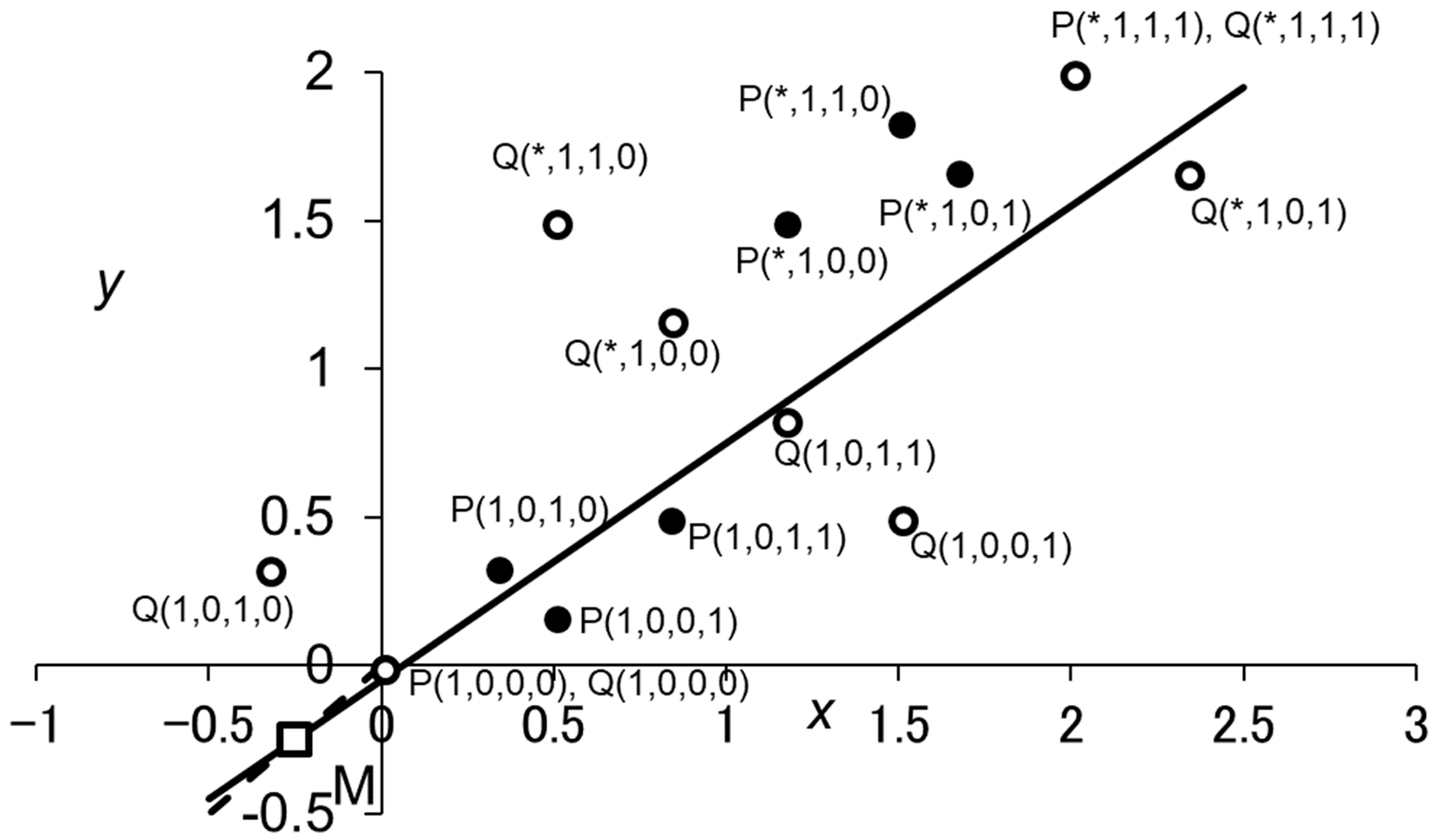
Figure A1.
Geometric representations of Inequalities (A34) and (A36) for . Each reactive strategy is represented by two points on the -plane, P() and Q(). The empty square represents point M, which is given by and on the line () (the broken line). The thick line is the “critical line,” which passes M and has the slope . For given strategy , Inequality (A34) is satisfied if and only if P() is below the critical line, showing that and are the only reactive strategies that are selectively favored when replacing a population of ALLD. Similarly, Inequality (A36) holds true if and only if Q() is below the critical line. Parameter values used are and . The asterisks indicate that the corresponding element of d can be either 0 or 1.

The slope of the line through points Qd and M gives the right-hand side of Inequality (A36). Thus, Inequality (A36) is met if and only if Qd is below the critical line as mentioned above. From Equation (A37), it is clear that holds for any Qd with , which means that Qd with is above the critical line, for the slope of the critical line is always smaller than one. Hence, the fixation probability of ALLD replacing a population of is larger than for any having . Figure A1 illustrates the case of , showing that ALLD is selectively disfavored when replacing a population of , ,, or . When holds true, the fixation probability of ALLD is equal to .
References
- Trivers, R. The evolution of reciprocal altruism. Q. Rev. Biol. 1971, 46, 35–57. [Google Scholar] [CrossRef]
- Axelrod, R.; Hamilton, W.D. The evolution of cooperation. Science 1981, 211, 1390–1396. [Google Scholar] [CrossRef]
- Joshi, N.V. Evolution of cooperation by reciprocation within structured demes. J. Genet. 1987, 6, 69–84. [Google Scholar] [CrossRef]
- Boyd, R.; Richerson, P.J. The evolution of reciprocity in sizable groups. J. Theor. Biol. 1988, 132, 337–356. [Google Scholar] [CrossRef]
- Nowak, M.A. Stochastic strategies in the prisoner’s dilemma. Theor. Popul. Biol. 1990, 38, 93–112. [Google Scholar] [CrossRef]
- Nowak, M.A.; Sigmund, K. The evolution of stochastic strategies in the prisoner’s dilemma. Acta Appl. Math. 1990, 20, 247–265. [Google Scholar] [CrossRef]
- Press, W.H.; Dyson, F.J. Iterated prisoner’s dilemma contains strategies that dominate any evolutionary opponent. Proc. Natl. Acad. Sci. USA 2012, 109, 10409–10413. [Google Scholar] [CrossRef]
- Stewart, A.J.; Plotkin, J.B. Extortion and cooperation in the prisoner’s dilemma. Proc. Natl. Acad. Sci. USA 2012, 109, 10134–10135. [Google Scholar] [CrossRef]
- Stewart, A.J.; Plotkin, J.B. From extortion to generosity, evolution in the iterated prisoner’s dilemma. Proc. Natl. Acad. Sci. USA 2013, 110, 15348–15353. [Google Scholar] [CrossRef]
- Stewart, A.J.; Plotkin, J.B. Collapse of cooperation in evolving games. Proc. Natl. Acad. Sci. USA 2014, 111, 17558–17563. [Google Scholar] [CrossRef] [Green Version]
- Hilbe, C.; Traulsen, A.; Sigmund, K. Partners or rivals? strategies for the iterated prisoner’s dilemma. Games Econ. Behav. 2015, 92, 41–52. [Google Scholar] [CrossRef] [PubMed]
- Hilbe, C.; Chatterjee, K.; Nowak, M.A. Partners and rivals in direct reciprocity. Nature Hum. Behaviour. 2018, 2, 469–477. [Google Scholar] [CrossRef]
- Nowak, M.A.; Sigmund, K. Tit for tat in heterogeneous populations. Nature 1992, 355, 250–253. [Google Scholar] [CrossRef]
- Nowak, M.A.; May, R.M. Evolutionary games and spatial chaos. Nature 1992, 359, 826–829. [Google Scholar] [CrossRef]
- Killingback, T.; Doebeli, M. Self-organized criticality in spatial evolutionary game theory. J. Theor. Biol. 1998, 191, 335–340. [Google Scholar] [CrossRef] [PubMed]
- Fudenberg, D.; Harris, C. Evolutionary dynamics with aggregate shocks. J. Econ. Theory 1992, 57, 420–441. [Google Scholar] [CrossRef]
- Nowak, M.A.; Sasaki, A.; Taylor, C.; Fudenberg, D. Emergence of cooperation and evolutionary stability in finite populations. Nature 2004, 428, 646–650. [Google Scholar] [CrossRef] [Green Version]
- Kurokawa, S.; Ihara, Y. Emergence of cooperation in public goods games. Proc. R. Soc. Lond. B Biol. Sci. 2009, 276, 1379–1384. [Google Scholar] [CrossRef] [Green Version]
- Kurokawa, S.; Wakano, J.Y.; Ihara, Y. Generous cooperators can outperform non-generous cooperators when replacing a population of defectors. Theor. Popul. Biol. 2010, 77, 257–262. [Google Scholar] [CrossRef]
- Kollock, P. Social dilemmas: The anatomy of cooperation. Annu. Rev. Sociol 1998, 24, 183–214. [Google Scholar] [CrossRef]
- Milinski, M.; Semmann, D.; Krambeck, H.J.; Marotzke, J. Stabilizing the Earth’s climate is not a losing game: Supporting evidence from public goods experiments. Proc. Natl. Acad. Sci. USA 2006, 103, 3994–3998. [Google Scholar] [CrossRef] [PubMed]
- Hauert, C.; Schuster, H.G. Effects of increasing the number of players and memory size in the iterated Prisoner’s Dilemma: A numerical approach. Proc. R. Soc. Lond. B Biol. Sci. 1997, 264, 513–519. [Google Scholar] [CrossRef]
- Taylor, M. Anarchy and Cooperation; Wiley: New York, NY, USA, 1976. [Google Scholar]
- Boyd, R.; Lorberbaum, J.P. No pure strategy is evolutionarily stable in the repeated prisoner’s dilemma game. Nature 1987, 327, 58–59. [Google Scholar] [CrossRef]
- Boyd, R. Mistakes allow evolutionary stability in the repeated prisoner’s dilemma game. J. Theor. Biol. 1989, 136, 47–56. [Google Scholar] [CrossRef]
- van Veelen, M. Robustness against indirect invasions. Games Econ. Behav. 2012, 74, 382–393. [Google Scholar] [CrossRef]
- van Veelen, M.; García, J.; Rand, D.G.; Nowak, M.A. Direct reciprocity in structured populations. Proc. Natl. Acad. Sci. USA 2012, 109, 9929–9934. [Google Scholar] [CrossRef] [Green Version]
- García, J.; van Veelen, M. In and out of equilibrium I: Evolution of strategies in repeated games with discounting. J. Econ. Theor. 2016, 161, 161–189. [Google Scholar] [CrossRef]
- Bonner, J.T. The Social Amoeba; Princeton University Press: Princeton, NJ, USA, 2008. [Google Scholar]
- Yip, E.C.; Powers, K.S.; Aviles, L. Cooperative capture of large prey solves scaling challenge faced by spider societies. Proc. Natl. Acad. Sci. USA 2008, 105, 11818–11822. [Google Scholar] [CrossRef] [Green Version]
- Packer, C.; Scheel, D.; Pusey, A.E. Why lions form groups: Food is not enough. Am. Nat. 1990, 136, 1–19. [Google Scholar] [CrossRef]
- Creel, S. Cooperative hunting and group size: Assumptions and currencies. Anim. Behav. 1997, 54, 1319–1324. [Google Scholar] [CrossRef]
- Stander, P.E. Foraging dynamics of lions in semi-arid environment. Can. J. Zool. 1991, 70, 8–21. [Google Scholar] [CrossRef]
- Bednarz, J.C. Cooperative hunting Harris’ hawks Parabuteo unicinctus. Science 1988, 239, 1525–1527. [Google Scholar] [CrossRef]
- Rabenold, K.N. Cooperative enhancement of reproductive success in tropical wren societies. Ecology 1984, 65, 871–885. [Google Scholar] [CrossRef]
- Pacheco, J.M.; Santos, F.C.; Souza, M.O.; Skyrms, B. Evolutionary dynamics of collective action in N-person stag hunt dilemmas. Proc. R. Soc. Lond. B Biol. Sci. 2009, 276, 315–321. [Google Scholar] [CrossRef]
- Bach, L.A.; Helvik, T.; Christiansen, F.B. The evolution of n-player cooperation—Threshold games and ESS bifurcations. J. Theor. Biol. 2006, 238, 426–434. [Google Scholar] [CrossRef] [PubMed]
- Souza, M.O.; Pacheco, J.M.; Santos, F.C. Evolution of cooperation under n-person snowdrift games. J. Theor. Biol. 2009, 260, 581–588. [Google Scholar] [CrossRef] [PubMed]
- De Jaegher, K. Harsh environments and the evolution of multi-player cooperation. Theor. Popul. Biol. 2017, 113, 1–12. [Google Scholar] [CrossRef]
- Taylor, C.; Nowak, M.A. Transforming the dilemma. Evolution 2007, 61, 2281–2292. [Google Scholar] [CrossRef]
- Nowak, M.A.; Tarnita, C.E.; Wilson, E.O. The evolution of eusociality. Nature 2010, 466, 1057–1062. [Google Scholar] [CrossRef]
- Allen, B.; Nowak, M.A.; Wilson, E.O. Limitations of inclusive fitness. Proc. Natl. Acad. Sci. USA 2013, 110, 20135–20139. [Google Scholar] [CrossRef] [Green Version]
- Allen, B.; Nowak, M.A. Games among relatives revisited. J. Theor. Biol. 2015, 378, 103–116. [Google Scholar] [CrossRef] [PubMed]
- Kurokawa, S. Payoff non-linearity sways the effect of mistakes on the evolution of reciprocity. Math. Biosci. 2016, 279, 63–70. [Google Scholar] [CrossRef] [PubMed]
- Kurokawa, S. Imperfect information facilitates the evolution of reciprocity. Math. Biosci. 2016, 276, 114–120. [Google Scholar] [CrossRef] [PubMed]
- Peña, J.; Lehmann, L.; Nöldeke, G. Gains from switching and evolutionary stability in multi-player matrix games. J. Theor. Biol. 2014, 346, 23–33. [Google Scholar] [CrossRef] [PubMed] [Green Version]
- Archetti, M.; Scheuring, I. Review: Game theory of public goods in one-shot social dilemmas without assortment. J. Theor. Biol. 2012, 299, 9–20. [Google Scholar] [CrossRef] [PubMed]
- Bomze, I.; Pawlowitsch, C. One-third rules with equality: Second-order evolutionary stability conditions in finite populations. J. Theor. Biol. 2008, 254, 616–620. [Google Scholar] [CrossRef] [PubMed] [Green Version]
- Wu, B.; García, J.; Hauert, C.; Traulsen, A. Extrapolating weak selection in evolutionary games. Plos. Comput. Biol. 2013, 9, e1003381. [Google Scholar] [CrossRef] [PubMed]
- Slade, P.F. On risk-dominance and the ‘1/3—Rule’ in 2X2 evolutionary games. IJPAM 2017, 113, 649–664. [Google Scholar] [CrossRef]
- Moran, P.A.P. Random processes in genetics. Math. Proc. Camb. 1958, 54, 60–71. [Google Scholar] [CrossRef]
- Deng, K.; Li, Z.; Kurokawa, S.; Chu, T. Rare but severe concerted punishment that favors cooperation. Theor. Popul. Biol. 2012, 81, 284–291. [Google Scholar] [CrossRef]
- Zhang, C.; Chen, Z. The public goods game with a new form of shared reward. J. Stat. Mech. Theor. Exp. 2016, 10, 103201. [Google Scholar] [CrossRef]
- Kurokawa, S.; Ihara, Y. Evolution of social behavior in finite populations: A payoff transformation in general n-player games and its implications. Theor. Popul. Biol. 2013, 84, 1–8. [Google Scholar] [CrossRef] [PubMed]
- Gokhale, C.S.; Traulsen, A. Evolutionary games in the multiverse. Proc. Natl. Acad. Sci. USA 2010, 107, 5500–5504. [Google Scholar] [CrossRef] [PubMed] [Green Version]
- Hirshleifer, J. From weakest-link to best-shot: The voluntary provision of public goods. Public Choice 1983, 41, 371–386. [Google Scholar] [CrossRef]
- Diekmann, A. Volunteer’s dilemma. J. Confl. Resolut. 1985, 29, 605–610. [Google Scholar] [CrossRef]
- Fischbacher, U.; Gachter, S.; Fehr, E. Are people conditionally cooperative? Evidence from a public goods experiment. Econ. Lett. 2001, 71, 397–404. [Google Scholar] [CrossRef] [Green Version]
- Kocher, M.G.; Cherry, T.; Kroll, S.; Netzer, R.J.; Sutter, M. Conditional cooperation on three continents. Econ. Lett. 2008, 101, 175–178. [Google Scholar] [CrossRef] [Green Version]
- Herrmann, B.; Thöni, C. Measuring conditional cooperation: A replication study in Russia. Exp. Econ. 2009, 12, 87–92. [Google Scholar] [CrossRef]
- Martinsson, P.; Pham-Khanh, N.; Villegas-Palacio, C. Conditional cooperation and disclosure in developing countries. J. Econ. Psychol. 2013, 34, 148–155. [Google Scholar] [CrossRef] [Green Version]
- Takezawa, M.; Price, M.E. Revisiting “the evolution of reciprocity in sizable groups”: Continuous reciprocity in the repeated n-person prisoner’s dilemma. J. Theor. Biol. 2010, 264, 188–196. [Google Scholar] [CrossRef]
- Nowak, M.A.; Sigmund, K. A strategy of win-stay, lose-shift that outperforms tit-for-tat in the prisoner’s dilemma game. Nature 1993, 364, 56–58. [Google Scholar] [CrossRef] [PubMed]
- Kurokawa, S. Persistence extends reciprocity. Math. Biosci. 2017, 286, 94–103. [Google Scholar] [CrossRef] [PubMed]
- Hayden, B.Y.; Platt, M.L. Gambling for gatorade: Risk-sensitive decision making for fluid rewards in humans. Anim. Cogn. 2009, 12, 201–207. [Google Scholar] [CrossRef] [PubMed]
- Scheibehenne, B.; Wilke, A.; Todd, P.M. Expectations of clumpy resources influence predictions of sequential events. Evol. Hum. Behav. 2011, 32, 326–333. [Google Scholar] [CrossRef] [Green Version]
- Wang, Z.; Xu, B.; Zhou, H.-J. Social cycling and conditional responses in the rock-paper-scissors game. Sci. Rep. 2014, 4, 5830. [Google Scholar] [CrossRef] [PubMed]
- Tamura, K.; Masuda, N. Win-stay lose-shift strategy in formation changes in football. EPJ 257 Data Sci. 2015, 4, 9. [Google Scholar] [CrossRef]
- Kurokawa, S. Evolution of cooperation: The analysis of the case wherein a different player has a different benefit and a different cost. Lett. Evol. Behav. Sci. 2016, 7, 5–8. [Google Scholar] [CrossRef]
- Bowles, S.; Gintis, H. A Cooperative Secies: Human Reciprocity and its Evolution; Princeton University Press: Princeton, NJ, USA, 2011. [Google Scholar] [CrossRef]
- Kurokawa, S. Does imperfect information always disturb the evolution of reciprocity? Lett. Evol. Behav. Sci. 2016, 7, 14–16. [Google Scholar] [CrossRef]
- Kurokawa, S. Evolutionary stagnation of reciprocators. Anim. Behav. 2016, 122, 217–225. [Google Scholar] [CrossRef]
- Kurokawa, S. Unified and simple understanding for the evolution of conditional cooperators. Math. Biosci. 2016, 282, 16–20. [Google Scholar] [CrossRef]
- Kurokawa, S. The extended reciprocity: Strong belief outperforms persistence. J. Theor. Biol. 2017, 421, 16–27. [Google Scholar] [CrossRef] [PubMed]
- Kurokawa, S.; Ihara, Y. Evolution of group-wise cooperation: Is direct reciprocity insufficient? J. Theor. Biol. 2017, 415, 20–31. [Google Scholar] [CrossRef] [PubMed]
Figure 1.
Functional forms of for various payoff assumptions. The horizontal and vertical axes represent , the number of cooperating individuals in a given round among the group members, and , a function of as defined by Equation (13), respectively. Parameter values used are and , (a) The conventional linear payoff assumption, Equations (19) and (20); and , (b) A non-linear payoff assumption, Equations (42) and (43); (c) A non-linear payoff assumption, Equations (20) and (52). .

Figure 2.
The effects of and on the identity of the best reactive strategy. The horizontal axis represents (0.001 to 0.161 with the interval of 0.02) and the vertical axis is (0.05 to 0.95 with the interval of 0.05. The fixation probabilities of strategies are obtained without assuming weak selection (i.e., using Equation (8). The parameter values used are , , , and .

Figure 3.
Relative fixation probabilities of all reactive strategies for the linear public goods game with . The horizontal axis represents , which is positive when (i.e., the fixation probability of a single mutant of strategy , when introduced in a population of ALLD, exceeds what is expected under neutral evolution), and is negative when the inequality is reversed. The strategies are aligned in the order of the fixation probabilities, which are calculated using Equation (9). Results for different value of are shown: (a) , (b) , and (c) . Other parameter values are , , and . The asterisks indicate that the corresponding element of d can be either 0 or 1. The order of the strategies is affected by .


Table 1.
The payoff matrix of the general n-player game.
| Strategy of the focal individual | ||||||
| A | ||||||
| B | ||||||
Table 2.
A list of the ten best reactive strategies for under the linear payoff assumption of Equations (19) and (20). Vector and the corresponding value of are given. Parameter values are , , , and .
Table 2.
A list of the ten best reactive strategies for under the linear payoff assumption of Equations (19) and (20). Vector and the corresponding value of are given. Parameter values are , , , and .
| Ranking | ||
|---|---|---|
| 1 | (1,0,0,0,0,0,0,1,1,1,1) | 40.39 |
| 2 | (1,0,0,0,0,0,1,1,1,1,1) | 38.14 |
| 3 | (1,0,0,0,0,0,0,0,1,1,1) | 36.35 |
| 4 | (1,0,0,0,0,0,1,0,1,1,1) | 34.1 |
| 5 | (1,0,0,0,0,1,0,1,1,1,1) | 31.85 |
| 6 | (1,0,0,0,0,0,0,1,0,1,1) | 30.06 |
| 7 | (1,0,0,0,0,1,1,1,1,1,1) | 29.59 |
| 8 | (1,0,0,0,0,1,0,0,1,1,1) | 27.81 |
| 8 | (1,0,0,0,0,0,1,1,0,1,1) | 27.81 |
| 10 | (1,0,0,0,0,0,0,0,0,1,1) | 26.03 |
© 2018 by the authors. Licensee MDPI, Basel, Switzerland. This article is an open access article distributed under the terms and conditions of the Creative Commons Attribution (CC BY) license (http://creativecommons.org/licenses/by/4.0/).
Share and Cite
MDPI and ACS Style
Kurokawa, S.; Wakano, J.Y.; Ihara, Y. Evolution of Groupwise Cooperation: Generosity, Paradoxical Behavior, and Non-Linear Payoff Functions. Games 2018, 9, 100. https://0-doi-org.brum.beds.ac.uk/10.3390/g9040100
AMA Style
Kurokawa S, Wakano JY, Ihara Y. Evolution of Groupwise Cooperation: Generosity, Paradoxical Behavior, and Non-Linear Payoff Functions. Games. 2018; 9(4):100. https://0-doi-org.brum.beds.ac.uk/10.3390/g9040100
Chicago/Turabian StyleKurokawa, Shun, Joe Yuichiro Wakano, and Yasuo Ihara. 2018. "Evolution of Groupwise Cooperation: Generosity, Paradoxical Behavior, and Non-Linear Payoff Functions" Games 9, no. 4: 100. https://0-doi-org.brum.beds.ac.uk/10.3390/g9040100
Note that from the first issue of 2016, this journal uses article numbers instead of page numbers. See further details here.