Homophily and Social Norms in Experimental Network Formation Games


1
Department of Economics, Simon Fraser University, 8888 University Drive, Burnaby, BC V5A 1S6, Canada
2
PPE Program, University of Pennsylvania, 313 Claudia Cohen Hall, 249 South 36th Street, Philadelphia, PA 19104, USA
*
Author to whom correspondence should be addressed.
Games 2018, 9(4), 83; https://0-doi-org.brum.beds.ac.uk/10.3390/g9040083
Submission received: 21 September 2018
/
Revised: 11 October 2018
/
Accepted: 16 October 2018
/
Published: 19 October 2018
(This article belongs to the Special Issue Games on Networks: From Theory to Experiments)
Abstract
:Field studies of networks have uncovered a preference to befriend people we perceive as similar according to some dimensions of our identity (“homophily”). Lab studies of network formation games have found that adherence to social norms of reciprocity and inequity aversion are also drivers of network choices. No study so far has attempted to investigate the role of both homophily and social norms in a controlled environment. At the beginning of our experiment, each player fills in a personal profile. Each player then views the profile of all other players and expresses a degree of perceived similarity between his/her profile and the profile of the other player. At this point, a repeated network formation game ensues. We find that: (1) potential homophily considerations triggered by the profile rating task did not measurably change the players’ behavior compared to the baseline; (2) reciprocity plays a significant role in the formulation of the players’ strategies, in particular lowering the probability that the player naively best responds to the network observed in the previous period. We speculate that reciprocation of past choices might be a more “available” aid in strategy-formulation than considerations related to the similarity of the other players.
JEL Classification:
C91; D85; D011. Introduction
Previous literature has tried to isolate the determinants of behavior observed in social networks. A robust finding is that people tend to choose friends who are similar to them, a phenomenon that the the literature since [1] calls “homophily”, the subject of a vast scholarship.1 In an influential study using data from American high schools, Currarini et al. [9] found that homophily is widespread, especially within the Caucasian and African-American subpopulations. The theoretical model presented in this paper shows that to generate homophily, one needs both biased preferences and a matching technology that is biased towards people with whom we share features. The authors of [10] found evidence in an all-girls school in Pasadena, CA, that the bigger the social distance between two friends, computed through the length of the shortest path between them, the less the “proposing friend” gives to a “receiving friend” in a dictator game. While features of the network are predictive of dictator giving, personal features are not. The authors found that personal features like ethnicity that the pupils share are instead important predictors of whether they state they are “friends”, again evidence of homophily.2
Homophily can only play a role in the interaction among heterogeneous players, i.e., players who differ along some socially significant aspect of their identity. The work in [13] surveyed different strategies in recent economic scholarship to model identity, the most influential attempt being perhaps that of [14], based on a utility function that includes, among other things, one’s identity or self-image (cf. also [15], discussing the problem of affiliation to multiple groups). Several recent contributions tried to spell out the way in which homophily and identity might shape network behavior. In [16], the payoff of the players explicitly depended on the social distance between the features of the players. The model of [17] generated, among other results, insights into the dynamics of homophily over the lifespan of a “networking” individual.
The existing experimental literature on network formation games has shown that adherence to social norms of reciprocity and inequity aversion are important predictors of the players’ behavior (cf., e.g., [18,19]). To the best of our knowledge, no experimental study has attempted to investigate the role of both homophily and social norms in network choices.3
In our experiment, each player fills in a profile (longer in Treatment 1, shorter in Treatment 2) where he/she can disclose demographic and hobby-related information to the other group members. Each player is then shown the profiles of the other players and is asked to express the degree of perceived similarity between the profile of each of the other players and his/her own profile. The players then repeatedly decide whether they wish to link or not to the other group members. The experiment is in discrete time, and all links are unmade at the end of each round. Links require no mutual consent, are insensitive to the presence of intermediaries and, once established, benefit both players, regardless of who has paid to create the link in a certain round (two-way flow of benefits). This network formation game was first studied by [24]. It shares some features with a social dilemma: each player prefers to be linked to the others, but has a preference for the others to pay for the links to be established.
We hypothesize that reciprocity and inequity aversion play a role in our experiment. After each round, the players see the full network, which shows all connections that were created in that round (and those that were not). An assessment of the other players’ intentions to link is therefore possible, a necessary intermediate step for reciprocity concerns to arise (cf. [25,26]). The display of the network in each round’s feedback stage also allows players to compute everyone’s payoff. Inequity aversion might arise following an assessment of the distance between one’s own and someone else’s (or the average) payoff.
A concern is whether our choice of network formation game, especially two-way flow of information, defaults inequity aversion and reciprocity to play a role in our experiment. Many possible networks are possible as a result of the strategic interaction, ranging from more egalitarian, when all players create a link, to highly asymmetric, as in the case in which one player links to everyone else (the “center-sponsored” star, in the language of [24]). The game we chose does not seem, therefore, to default inequity aversion to play a role. The game we chose offers, instead, somewhat unconducive conditions for reciprocity to arise, especially if subjects learn naively (i.e., they best respond to the network observed in the previous period, assuming everyone else confirms his/her choice). If reciprocity is observed nevertheless, this might be taken as further evidence of the strength and stability of reciprocity in the set of human motivators (cf., e.g., [27,28]).
Homophily might also play a role, as the participants have access to the profiles of the other players throughout the experiment. The most obvious hypothesis is that players will link preferably to those they perceive as similar. Our analysis is exploratory regarding which of the three forces (homophily, reciprocity or inequity aversion) is prevalent in our controlled environment.
We find that similarity does not change in any measurable way the behavior of the players. Previous studies have found that heterogeneity induced by the experimenter by breaking the full symmetry of the players promotes convergence to equilibrium ([29]). Heterogeneity linked to personal features of the participants seems, instead, not to be equally “available”4 in strategy formulation. Reciprocity considerations discourage naive best responses. In some empirical specifications of our regression model, players are more likely to create a link to an opponent if that opponent created a link in the previous period. Inequity aversion does not seem to have a measurable impact on the players’ choices.
2. Results
2.1. The Dataset
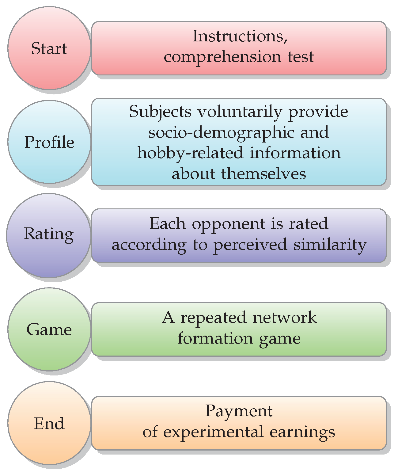
While adherence to social norms is a traditional territory of inquiry for experimental economics (cf. [31] and the references cited therein), studying homophily in the laboratory is a novel aspect of our study, and it presents several challenges. The experimenter needs to ensure that the privacy of the participants’ features and choices is preserved. Relatedly, the students are randomly matched into groups of strangers and learn of potential common traits or tastes in the lab. Homophily concerns might therefore only arise after the experimental groups are formed. The compromise solution we devised was to allow the students to release to the other group members information about themselves, using questionnaire responses. The design of our treatment studies is summarized in Figure 1: following the usual formalities (instructions and comprehension test), groups are randomly formed. The participants then fill in a profile. After, each participant rates each opponent in terms of perceived similarity. Finally, the participants play a repeated network formation game. The experiment concludes with the payment of the experimental earnings. The control study is a repeated network formation game, without profile and rating stages.
We recruited 90 Simon Fraser University students to participate in our study. Twenty subjects played our TG1 (four independent groups), our treatment study featuring a longer profile; 30 subjects the TG2 (six independent groups), our treatment study featuring a shorter profile; and 40 subjects the CG (eight independent groups), the control study featuring no profile (and no rating). Each group interacted for 20 rounds, with fixed IDs. No subject participated more than once in any of our sessions. Sessions lasted on average 90 min, and subjects earned on average 15 Canadian dollars, including a show-up fee. We have evidence that the rating was done consistently in TG1 and TG2, as measured by the correlation between our two measures of similarity (number of attributes shared and proximity of the rated participant’s attributes to the rater’s); we have evidence also that the perception of similarity is mutually shared, i.e., there is a high correlation between i’s rating of j and j’s of i. The average degree of similarity in each group was approximately the same, and the sessions were gender-balanced.
2.2. Descriptive Statistics
Table 1 shows the descriptive statistics of the three key dependent variables: the decision to create a link (), whether two players are directly connected (i.e., either i linked to j or j linked to i) and whether the decision in a round was a naive best response to the network observed in the previous period (bestresp5). As explained further below, each participant ( for short) had four s in each round, which tell us whether that participant had linked or not to each of the four opponents in each round. Standard errors were clustered at the level of each participant.
Even in an environment like ours in which the marginal benefit of creating a link in an empty network is higher than the marginal cost (cf. Equation (5) in Section 4 below), participants chose on average not to create a link. This behavior was a result most likely of the belief that a path would exist to other players even if one paid for no link. The probability that any two participants were directly connected was roughly 50%. The proportion of naive best responses was consistent with earlier findings ([32]).
In order to gain insights into the effectiveness of our manipulation (the profile and the rating), we grouped responses from the two treatments together and conducted a two-sample Wilcoxon rank-sum (Mann–Whitney) test to verify whether the medians of , connected and bestresp were the same in all treatments vs. the control. The null was rejected in all three cases (z = −3.525, −3.354 and 2.730, respectively), a first sign of the effectiveness of our manipulation (profile and rating).
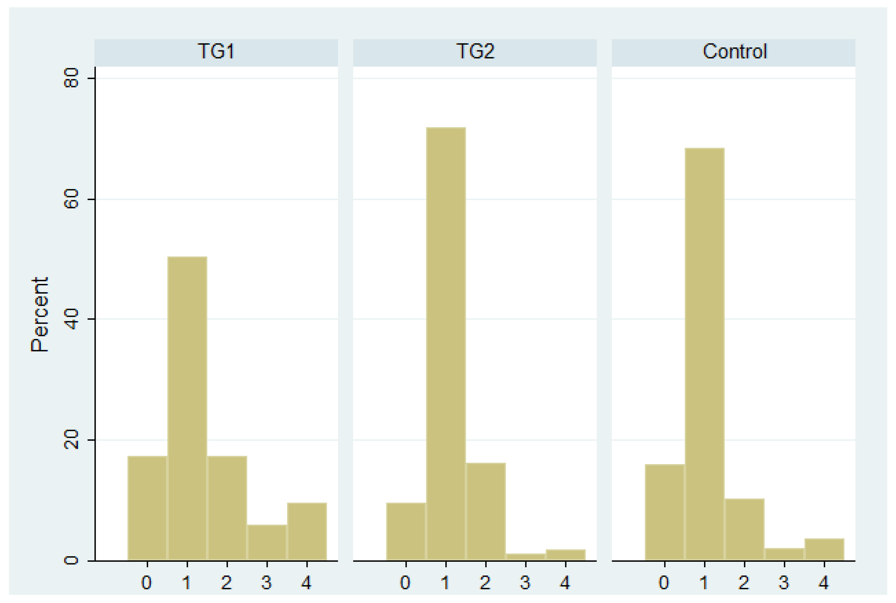
Figure 2 is a histogram of the average number of links formed by the players in each round, for the two treatments and the control. The modal choice is to form one link in the three subplots.
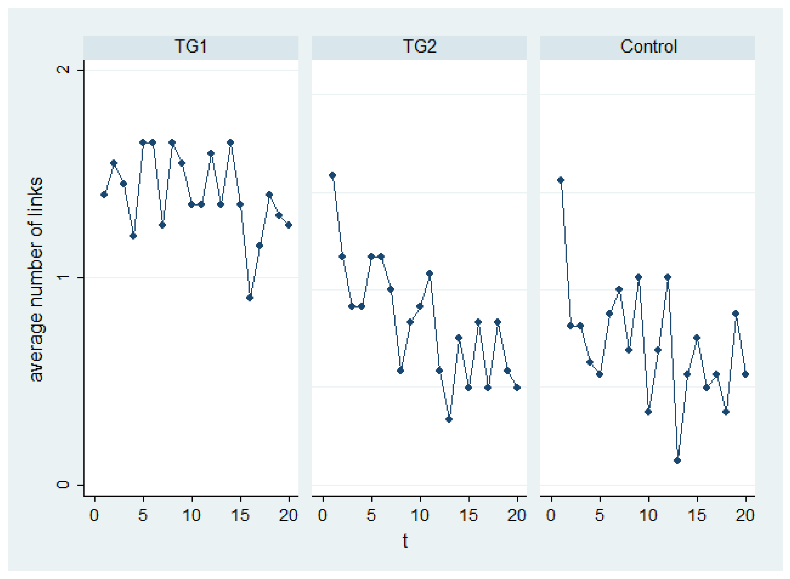
Figure 3 shows the average number of links created in each period t, where the mean is across the players in each round of play. Although no clear trend is apparent in TG1, in TG2 and the Control a tendency is apparent to choose fewer links in the final rounds compared to the initial rounds.
We now try to explain the behavior of the players through the measure of similarity we collected at the beginning of the experiment, as well as through reciprocity and inequity aversion considerations. For this analysis, only the data from TG1 and TG2 are useful, as the Control did not include the profile and rating stages. The sample size for regression analyses was therefore restricted to 50 participants.
2.3. Constructing a Panel
Participants in our experiment were observed repeatedly making choices. The most natural choice of the class of estimators for this dataset was panel data estimators. The obvious choice for the time identifier of our panel was the round number. The choice of the individual identifier was less obvious. In each round, every participant (abbreviated as pers) made four binary choices, i.e., whether one wants to link or not to the four opponents each player faces in his/her group. Panel data analysis required that each individual identifier be observed once in each time identifier. To take care of this constraint, we assigned to every four different ’s. The individual identifier of our panel was . considered each participant in relation to each opponent. Each had therefore four ’s. These “couples” were fixed for the purpose of estimation (i.e., each was observed for 20 rounds of play).
2.4. The Data Generating Process
A first way to specify our regression model is shown in Equation (1):
The dependent variables (y) are the decision to by (; 6) and whether the decision taken was a naive (; 7). is the number of personal features the two players shared, as expressed by each in the rating; is the average degree of similarity to the vector of personal features of the other player, expressed also in the rating stage of the experiment (Likert-scale from one, very dissimilar to five, very similar, averaged for all dimensions that were rated to end up with a single number); is a multiplicative interaction term of and that we added to account for the high correlation between the two measures of similarity; is a dummy variable that was equal to one if j linked to i in period ; is a dummy variable equal to one when the difference between i’s payoff at and the average payoff in his/her group at was positive (zero in all other cases); is a dummy variable for TG1: captures the marginal effect of having a longer questionnaire and evaluating the other player on several extra dimensions.
Model (1) allows each cross-sectional unit () to have a different intercept. If one makes the additional assumptions that and the error term are i.i.d., we have the well-known random effects (RE) model ([33], p. 700).
An alternative specification of our data generating process (DGP) is the so-called fixed effects (FE) model (Equation (2)). This model estimates a transformed Equation (1) without and the time-invariant regressors (cf. [33], p.750).
2.5. Challenges to Consistent Estimation
Our dependent variables of interest are binary. A choice must be made between linear probability models available for panel data and non-linear estimation methods for panel data (such as probit). The estimated coefficients retain the traditional marginal-effect interpretation only in the case of linear probability models, and thus, this is our preferred estimation method.8
Some of our key regressors, like the measures of similarity, are time-invariant. For the estimation of the coefficients of these time-invariant variables, we can only rely on the RE (Equation (1)) or the mixed (Equation (4)) models.
To obtain consistent estimates of the parameters of interest, the RE model requires the assumption of strong exogeneity: . This assumption can be tested through a robust version of the Hausman test, detailed below. Furthermore, if Model (1) is correctly specified, then the RE estimator is consistent and asymptotically efficient. The FE estimator is always consistent, possibly though not the most efficient because of the transformation it requires (cf. [33], pp. 716–717).
The mixed model (Equation (4)), sometimes also called “hybrid” or “correlated random effects”, gives us fixed-effects estimates of time-varying variables, but allows also the inclusion of time-invariant variables, estimated in a random effects framework. The mixed approach might outperform FE and RE in finite samples ([37]). The mixed model uses the logic of the Hausman–Taylor model (cf. [33], p. 761), in which the researcher must make the difficult choice of which regressors are endogenous (with respect to the unobserved effects) and which are exogenous. The assumption of Model (3) is that all time-varying regressors (reciprocity and inequity aversion) are endogenous and all time-invariant regressors (the measures of similarity) are exogenous (cf. [33], p. 761). This assumption appears plausible in our setup.
A standard Hausman test can be used to check the plausibility of the additional assumptions of the RE model (compared to the FE model). A shortcoming of this test is that it requires the and to be i.i.d., an assumption that does not hold “if cluster-robust standard errors for the RE estimator differ substantially from default standard errors” ([38], p. 261). Our panel suffers most likely from clustering problems at the level of the participant. Two (equivalent) robust Hausman tests for data affected by clustering issues are available and detailed in [38] (p. 262) and [39], respectively. These tests take explicitly into consideration clustering problems in the panel and are based on the procedure described in [40]. This a test of the overidentifying restrictions in the RE model, considering the less onerous orthogonality restrictions of the FE model. If the test is in the rejection area, this is a rejection of the over-identifying restrictions of the RE model and evidence in favor of FE. The Hausman test with as the dependent variable rejects the null hypothesis of exogeneity of the random effects (Sargan–Hansen statistic 97.97, p < 0.01). We also reject the null when bestresp is the dependent variable (Sargan–Hansen statistic 9.60, p < 0.01). The Hausman test results alert us to the risks of drawing inferences only based on the RE model, but should not be taken as definite evidence against RE estimates. The Hausman test might not provide reliable guidance on which approach to follow ([41]). It has been observed that occasionally, it is preferable to use RE when this involves a small enough bias, rather than choosing the less precise FE estimator ([41]). The approach we follow in the next section is to display the output using RE, FE and mixed estimation.9
Another challenge is the estimation of the asymptotic variance matrix for inference. Every participant has four ’s, requiring clustering at the level of pers.10 We use the bootstrapping method to estimate the asymptotic variance matrix, correcting for clustering in pers.11 Simulation methods for the standard errors are available in the statistic software for both linear and nonlinear (probit and logit) estimation methods, while clustering is only available for linear estimators, another reason why we concentrate on linear estimators. The number of clusters (50) seems congruous.
2.6. Estimation Results
Using as the dependent variable (Table 2), the two main similarity measures are positively, but insignificantly correlated with the decision to link in all three models.
We found evidence of reciprocity motives playing a role in increasing the propensity to link from RE estimation. As a robustness check, we have also used the single personal features the subjects shared (or not) as regressors (for example, if the subjects claimed to be of the same gender), instead of the aggregate measure that measured the number of personal features the subjects claimed to share. These regressors were also not significant. As a further robustness check, we used the observations from Round 1 only (a cross-section), but did not find evidence of similarity driving choices, even in the first round. Furthermore, being better off in round did not measurably impact round t behavior.
Using as the dependent variable (Table 3), we found evidence that reciprocity considerations negatively affect the decision to naively best respond to the network observed in the previous period, in all three models.12 Possible explanations for this finding are i’s desire to reciprocate; or the fear that j might stop paying to form a link, because of inequity aversion or spite. The explanatory power of our regression models was generally low, a result that was due both to the exclusion of unnecessary variables that would raise the R (mixed estimation, which augments the model with the averages of time-varying regressors, had in fact much higher R), but also to the very high degree of experimentation that took place in game, as shown in Figure 3.
2.7. Relation to Previous Literature
Previous studies found that with a two-way flow of benefits and homogenous players, the players rarely achieved full coordination on a Nash equilibrium ([18,32]). The authors of [18] explained this finding as a result of social norms of symmetry interfering with naive best response dynamics. Asymmetry in their paper resulted from one player paying for all links, while all others enjoyed the benefits of the network, without incurring any cost. This network was an equilibrium of the network formation game with two-way flow of information and no decay, as proven by [24], but it resulted in an inequitable distribution of payoffs between the sponsor of all links and the other players. The role of inequity remained elusive in our experiment. There were, however, differences in design between [18], featuring homogeneous players, and our study.
The authors of [29] argued that the low frequency of Nash equilibrium networks in Falk and Kosfeld’s study was caused by the homogeneity of the players that aggravated the problem of coordinating. The authors broke the homogeneity by granting: one player the possibility of forming links at a cheaper rate in one treatment (low cost); one player higher benefits when other players link to him/her (high value); two players per group the “high-value” feature; one player the low-cost feature and another the high-value feature, in each group. The introduction of heterogeneity significantly increased the likelihood of a Nash equilibrium.
Heterogeneity of the type introduced by [29] cannot give rise to homophilous behavior, as heterogeneity was created through an experimental manipulation. In our paper, heterogeneity was brought into the lab by the experimental subjects, and it derived from the naturally occurring variability in the identity of the players. This heterogeneity was arguably closer to real-world patterns, where it is hard to imagine the existence of low-cost or high-benefit individuals from inception. We suspect that in situations in which the special player had to emerge endogenously, the effect of heterogeneity on convergence to an equilibrium might be significantly more nuanced than in [29].
3. Discussion
In this paper, we study the role of homophily and adherence to social norms in a novel experimental framework. Table 4 contains a summary of the hypothesized signs for the coefficients of interest in Equation (1) (cf. Section 4) and our findings. While our hypotheses regarding the way in which reciprocity interacts with linking choices and naive best responses are confirmed, the effects of inequity aversion and homophily are elusive.
Abstracting from considerations related to the particular population our experimental subjects were sampled from, a possible explanation for our null finding regarding homophily is that the computational difficulty of the network formation game shifted the players’ focus from the personal features of the players to their immediate past choices, shown at the end of every round. Notwithstanding our efforts to make the personal features of each group member easy to retrieve during the experiment, personal features might not have been “available” to the participants, occupied in strategy formulation in a complex repeated game with four opponents. In the experiment, subjects decided how to allocate their time between at least three different activities. They could recall or revisit by clicking on the appropriate button on the screen the personal information provided by the other players; they could study the previous choices and payoffs of the other players; or simply experiment. It is likely that the last two activities absorbed the attention of the players. In a possible extension of our study, participants could buy information on the other players and information on the strategy they plan to adopt in the network formation game. In our current experimental design, all information, personal and about past choices of the other players, was provided for free. This amendment would allow us to measure the demand of the participants for information about the other players.
Another possible explanation for our finding that the players’ decisions were not affected by similarity considerations is the lack of a biased matching technology. In the theoretical model of homophilous behavior in [9], biased preferences are not sufficient to generate widespread homophilous behavior. One also needs a biased matching technology, i.e., a coordinating device that increases the probability that two similar individuals meet above pure chance levels. This type of situation is more likely to arise in field studies, where similar subjects congregate in clubs or associations, rather than in lab studies where students are randomly assigned to experimental groups. Coupling the possibly inborn biased preferences of the experimental subjects with a design that features a biased matching technology seems a promising approach to generate homophilous behavior in the lab in the future.
Another set of concerns is directly attributable to the way our network formation game was specified, with particular reference to the two-way flow of benefits feature. If a player desires to link to another player who is rated as similar, he/she needs also to consider whether a path to that player will exist through links paid by others. Furthermore, it is possible that the profile and rating manipulations were excessively conservative and that instead having the participants exchange “relational goods” (cf. [42]), through a direct meeting at the end of the experiment for example, might rescue homophily. This type of manipulation would, however, violate the standard anonymity conditions in which economic experiments are usually carried out.
We find evidence that (naively) best responding to the previous period network and reciprocating past choices are in a negative relation. It is possible that in our study, the subjects were trying, in subtle ways, to reach an equitable division of the burden of creating a link, by trying for example to alternate linking decisions, out of a concern for a norm of reciprocity. Institutions might help in this coordination problem ([43]). Possible ways to study the players’ desire to share the burdens of linking would be: (i) the introduction of a bargaining stage to determine the division of the cost of linking; (ii) the introduction of side payments among the players, which could also bring further evidence of the presence of reciprocity concerns of the players when making linking decisions.
4. Materials and Methods
We studied two treatments and one control. Treatment 1 (TG1) was divided into three phases. In Phase 1, subjects were assigned randomly to groups composed of 5 players. The subjects were identified in the course of the session only by a random ID, which was visible to all other group members. Subjects interacted with the same group members for the entire duration of the session. After that, the experimenter read the instructions aloud13, and the subjects took a test to ensure that they understood the way payoffs were calculated (explained further below). Answers were checked individually by the experimenter.
In Phase 2, subjects filled in a questionnaire using a web-based application. Subjects could provide information on their gender, age, languages they spoke, their major, favorite sport, political views, favorite singers, whether the subject usually had an impulsive (vs. reflective) attitude when making decisions, whether the respondent devoted time to volunteering activities, length of Facebook use per day, frequency with which the participant talked to his/her family per week and number of text messages sent.14 We refer to each answer in the questionnaire as a “personal feature” of the subject and the vector of personal features as his/her “profile”. Subjects could not reveal their identity or name, as all their questionnaire answers were picked from a drop-down menu with predetermined options. Subjects could decline to provide an answer to each question by simply choosing the “Prefer not to say/None of the above” option provided for each question. Through their profile, the participants could share with the other group members basic information on their demographic characteristics, hobbies and some proxies for sociability. The subjects knew that their profile would be rated by the other players, and there was no incentive for them to report their features truthfully. We cannot, therefore, exclude that the players provided answers that they thought would be popular.15
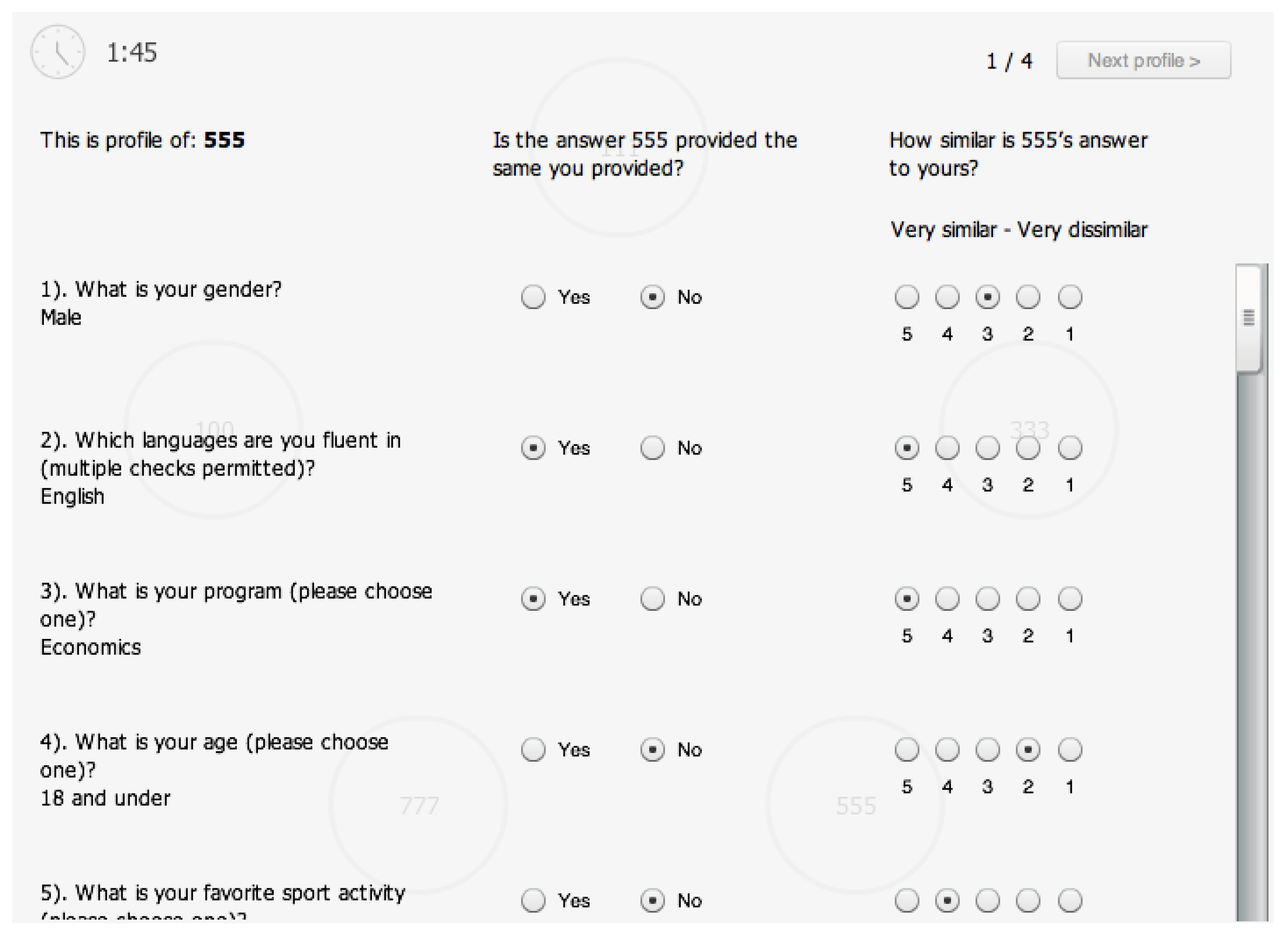
Then, the subjects were asked to “rate” the profiles of the other group members. For each subject in his/her group (identified by experimental ID), the “rater” had to answer whether each single personal feature of the “rated” was shared; the rater also expressed a degree of similarity between the personal feature of the other player and his/her feature, on a Likert scale from 1 to 5, for each single question of the questionnaire. Figure 4 is a screenshot of part of the page where subjects performed the rating. The rating of all players in one’s group concluded Phase 2 of the experiment.
In Phase 3, the subjects were asked to choose whether they wanted to link to the other players in their group. The costs of link formation were incurred only by the person who initiated the link (cf. [24]). Establishing the relationship required no mutual consent. The benefits of the relationship accrued, however, to both players i and j, regardless of who paid for the link to be established, a feature known as two-way flow of benefits (cf. [24], p. 1182). In our experiment, if agent was linked with some other agent via a sequence of intermediaries , then the benefit that derived from being indirectly linked to was insensitive to the number of intermediaries, a feature known as no decay. The no decay feature of the experiment simplifies the computation of payoffs greatly in each round of our experiment. Introducing at this point some simple notation allows us to write the payoff function for the network formation game our participants played.
Let be the set of players. A strategy of player was a vector , where , . i had a link to j if . Given two-way flow of benefits, allowed both i and j to benefit from the link. We call the set of strategies of player i and the space of pure strategies of all the players. The strategies of all the players, summarized in the strategy profile gave rise to a network. The closure of g, denoted , is defined by for each . was the number of players i had a path to (the path can have an arbitrary number of intermediaries given no decay), not including i himself. denotes the number of players to which i paid to link. The simplest linear payoff function for this game, first used by [24], reads as follows:
where c is the cost of forming a link, set at 0.5 in our experiment; and the benefit is given by the number of agents to which i has a path. Because of its simplicity, this payoff function has been used in earlier experimental papers (e.g., [18]). Importantly, this payoff function allowed us not to impose on the subjects a preference structure, in the form of homophily preferences (like, e.g., in [16]) or inequity averse/intention-based preferences (as, e.g., in [26] or [45], respectively). Whether homophily, social norms, or both, drove choices is a question we investigate empirically in our controlled environment.
Subjects created a link by clicking on the ID of the other player, an input that created a line on the screen between the link initiator and the link receiver. The link could be unmade by clicking again on the ID of the other player. Each participant could retrieve at any point during the game the profile of the other participants by clicking on a “profiles” button located on the top-right corner of the screen.
Once all players made their choices, the subjects were shown the strategy profile g, as illustrated in Figure 5. Then, subjects manually computed their payoff and recorded it on a piece of paper provided. The manual calculation of the payoffs was a way in which we tried to ensure that subjects paid attention to the network formed in each period. If payoffs were instead simply presented to the subjects, as customarily done in laboratory studies, subjects could have completely ignored the previous-period network in the formulation of their next period response. Although subjects computed their payoffs, payments were made at the end of the session based on the experimenter’s calculation, as explained in the instructions.
The players had a time limit of four minutes to make their decisions, after which the system imputed a “No links” decision to the player. The subjects repeated the linking decisions for 20 rounds. At the end of the 20th round, we randomly selected one round, and subjects were paid according to their earnings in that round, with the exchange rate set at 1 point = $5 Canadian. Participants also received a show-up fee of $7.
Our second treatment (TG2) is a simple variant of TG1. The questionnaire we used in Phase 2 of the experiment was shorter, and it included only information on age, languages spoken, gender and major. The experiment was in all other regards the same as TG1. We devised TG2 to address the concern that the 12-item questionnaire we used in TG1 might have provided an excessive amount of information that the subjects did not find very valuable. The four questions that were included in the TG2 questionnaire were chosen through a non-incentivized survey of Simon Fraser University undergraduate students () in which we asked what the selection criteria they used in their day-to-day friendship decisions were. The four answers that appeared most often were used in the TG2 questionnaire.
Our Control (CG) lacks Phase 2 of TG1, i.e., the questionnaire and the rating. After Phase 1, subjects play the network formation game. This study is essentially a replication of some of the treatments in [18,32] although with different cost and benefit parameters that affect the comparability of their findings and ours. The purpose of the control was to gain insights into the determinants of network formation choices in the absence of any possible role of homophily.
There were three hypotheses we wished to subject to experimental testing:
Hypothesis 1.
The similarity between two players predicts whether the two players are directly connected.
We hypothesize that players perceived as similar are linked to more often. Picking links by perceived similarity is a sound strategy if it is true that subjects have homophilous preferences, which, as we have seen, is a robust finding in the field literature on networks.
Hypothesis 2.
A player is more likely to create links in period t if he/she earned more than the group average in round .
This hypothesis is motivated by the likely presence of inequity aversion motives in the players, as already documented by [18]. If a player earned more than the group average in the previous round, he/she is likely to increase the number of links he/she pays for in the next round to reduce payoff differences. Similarly, if the player earned less than the group average, he is likely to reduce the number of links he/she pays for. This effect must be further checked by excluding from the empirical analysis the instances in which the player earned zero in the previous round (i.e., he/she paid for no link and no player linked to him/her). In this case, the player is at a payoff-disadvantage compared to everyone else (unless everyone else earned zero too, the case of an empty network), and the hypothesis would predict a reduction of the number of links. This is clearly impossible in the case of zero links. Furthermore, an inequity-averse player in this case would rather increase links to try to reduce the payoff differences.
Hypothesis 3.
Player j’s decision to create a link to player i in round t is positively associated with i’s decision to link to j in round .
We hypothesize that players adhere to a social norm of reciprocity. This norm is fact, hard to reconcile with the the learning algorithm postulated by [24], i.e., naive best response. If subject i (he) believes that subject j (she) will link, based on her previous-round choice, then i has no incentive to link to j, and therefore, i would naively best respond by not positively reciprocating j’s choice. If on the other hand, i believes that j will not link to him, and player i expects not to have any path to j, then a naive best responding player i has incentives to link to j, and therefore, i would rationally not negatively reciprocate j’s choice of not linking in the previous period, creating instead a link. We expect that many subjects will forgo naive best responding and will reciprocate past choices, positively (linking to j if j made a link in period ) or negatively (i.e., avoiding making a link to j if j did not create a link in the previous period). If reciprocation and naive best responding are indeed alternative learning algorithms in our repeated network formation game, then we should expect to find a negative relation between the two variables. This would bring further evidence that some players do not learn to best respond, but rather they learn, or perhaps are hard-wired, to return kind and unkind acts of the other players (cf. [26]), “in kind”.
Author Contributions
Conceptualization, G.D. and J.A. Data curation, G.D. Formal analysis, G.D. Funding acquisition, J.A. Investigation, G.D. Methodology, G.D. and J.A. Software, J.A. Supervision, J.A. Visualization, G.D. Writing, original draft, G.D. Writing, review and editing, G.D.
Funding
This research was funded by the Community Trust Endowment Fund Grant Number 31-788021.
Acknowledgments
We would like to thank for useful discussions: Brice Corgnet, Greg Dow, Erik Kimbrough, Chris Muris and Ruth Tacneng. Anton Krutov provided software assistance. The usual disclaimer applies.
Conflicts of Interest
The authors declare no conflict of interest.
Abbreviations
The following abbreviations are used in this manuscript:
| MDPI | Multidisciplinary Digital Publishing Institute |
| DOAJ | Directory of open access journals |
| TLA | Three letter acronym |
| LD | linear dichroism |
Appendix A. Instructions: TG1 and TG2
Welcome to this experiment in decision-making. Please read these instructions carefully. Throughout the experiment you are not allowed to communicate with other participants in any way. If you have a question please raise your hand. One of us will come to your desk to answer it confidentially.
During this experiment you will earn experimental points, on the basis of your own decisions and the decisions of all other players in your group. At the end of the experiment, one round of play will be picked at random, and everybody will be paid according to his/her earnings in that round. You will be paid according to the system’s calculation of your payoff. The exchange rate will be: 1 experimental point = $5. You will be paid your earnings privately and confidentially at the end of the experiment. You have already earned 1.4 experimental point ($7) for your participation.
In this experiment, you will play with four other players, randomly chosen by the system from those in the room at this time. For the purposes of this experiment you will be identified only by the random username you were assigned. Some of the usernames are masculine, some are feminine: this bears no relationship to the actual gender of the player.
As soon as we finish reading these instructions, you will be asked to enter your username on a webpage. Notice that the username is the code you randomly picked, and it is NOT your real name.
Then, you will move to TASK 1:
TASK 1: you will fill in a questionnaire asking you to provide, on a voluntary basis, some information on yourself. This information makes up your “Profile”.
Upon completion of TASK 1, you will move to TASK 2:
TASK 2: you will rate the Profiles of all other players in your group. More details on the rating system will be provided on the screen.
Upon completion of TASK 2, you will move to TASK 3:
TASK 3: here you will decide whether to link ti other players in your group, and with whom to link. You will take this decision for 20 times. The link(s) you make in a particular round are valid for that round only. In order to create a link to another player, you need to click with your mouse on his/her username. The choice can be undone by clicking for a second time on the username of the player.
You can make any number of links (0, 1, 2, 3 or 4). All subjects are identified through their usernames.
You can be “directly linked”, “indirectly linked” or “not linked” with any other member of your group. You are “directly linked” with another player if:
- you make a link to that player, or
- if that player makes a link to you, or
- if both of you link to each other.
Throughout the experiment we call Neighbors the people in your group that you are directly linked with. You are “indirectly linked” with another player if that player is not your neighbor but there is a sequence of links between you and that player.
If there is no sequence of links between you and another player then you are “not linked” (neither directly nor indirectly) to that player.
For each (direct) link that you make you have to pay some cost: 0.5 experimental points. You also benefit from being connected with other players: your benefit is equal to the number of people you are directly or indirectly linked to. Other players also benefit from the number of direct and indirect links they have (including their links with you).
You do not incur any cost for the links that other players make and other players do not incur in any cost for the links that you make.
Notice that there is a possibility that you are linked with the same player in more than one way. However, you only benefit once from being linked to this player.
After everybody in your group has made his/her choice, you will be shown everybody’s choices. An arrow starting from you pointing to another player (⟶) means that you have paid to link to that player. An arrow starting from another player and pointing towards you (⟵) means that that player has paid to link to you. A leftright arrow (⟷) between you and another player means that you have paid to link to the other player, and so did he/she to you.
You will then be asked to compute your earnings in that round based on the display of choices of yours and of all other group members.
The table below will help you in calculating your per-round earnings.
| Number of links you make | ||||||
| 0 | 1 | 2 | 3 | 4 | ||
| 0 | 0 | - | - | - | - | |
| 1 | 1 | 0.5 | - | - | - | |
| Number of people you are linked to | 2 | 2 | 1.5 | 1 | - | - |
| 3 | 3 | 2.5 | 2 | 1.5 | - | |
| 4 | 4 | 3.5 | 3 | 2.5 | 2 | |
The missing numbers in the table are due to the fact that you are always connected to at least the number of people you have paid to link to.
Notice that at all points during the experiment you are able to retrieve the profiles of the other players by clicking on the PROFILES button on the screen.
At the end of each round, please compute your earnings and record them on the sheet labelled “Record of Earnings”, which is on your desk.
In each round, your linking decisions have to be made within 4 min. If you have not taken any decision by then, the system will input a “no link chosen” decision.
Appendix B. Instructions: Control
Welcome to this experiment in decision-making. Please read these instructions carefully. Throughout the experiment you are not allowed to communicate with other participants in any way. If you have a question please raise your hand. One of us will come to your desk to answer it confidentially.
During this experiment you will earn experimental points, on the basis of your own decisions and the decisions of all other players in your group. At the end of the experiment, one round of play will be picked at random, and everybody will be paid according to his/her earnings in that round. You will be paid according to the system’s calculation of your payoff. The exchange rate will be: 1 experimental point = $5. You will be paid your earnings privately and confidentially at the end of the experiment. You have already earned 1.4 experimental point ($7) for your participation.
In this experiment, you will play with four other players, randomly chosen by the system from those in the room at this time. For the purposes of this experiment you will be identified only by the random username you were assigned. Some of the usernames are masculine, some are feminine: this bears no relationship to the actual gender of the player.
As soon as we finish reading these instructions, you will be asked to enter your username on a webpage.
Then the experiment will start. You will decide whether to link to other players in your group, and with whom to link. You will take this decision for 20 times. The link(s) you make in a particular round are valid for that round only. In order to create a link to another player, you need to click with your mouse on his/her username. The choice can be undone by clicking for a second time on the username of the player.
You can make any number of links (0, 1, 2, 3 or 4). All subjects are identified through their usernames.
You can be “directly linked”, “indirectly linked” or “not linked” with any other member of your group. You are “directly linked” with another player if:
- you make a link to that player, or
- if that player makes a link to you, or
- if both of you link to each other.
Throughout the experiment we call Neighbors the people in your group that you are directly linked with. You are “indirectly linked” with another player if that player is not your neighbor but there is a sequence of links between you and that player.
If there is no sequence of links between you and another player then you are “not linked” (neither directly nor indirectly) to that player.
For each (direct) link that you make you have to pay some cost: 0.5 experimental points. You also benefit from being connected with other players: your benefit is equal to the number of people you are directly or indirectly linked to. Other players also benefit from the number of direct and indirect links they have (including their links with you).
You do not incur any cost for the links that other players make and other players do not incur in any cost for the links that you make.
Notice that there is a possibility that you are linked with the same player in more than one way. However, you only benefit once from being linked to this player.
After everybody in your group has made his/her choice, you will be shown everybody’s choices. An arrow starting from you pointing to another player (⟶) means that you have paid to link to that player. An arrow starting from another player and pointing towards you (⟵) means that that player has paid to link to you. A leftright arrow (⟷) between you and another player means that you have paid to link to the other player, and so did he/she to you.
You will then be asked to compute your earnings in that round based on the display of choices of yours and of all other group members.
The table below will help you in calculating your per-round earnings.
| Number of links you make | ||||||
| 0 | 1 | 2 | 3 | 4 | ||
| 0 | 0 | - | - | - | - | |
| 1 | 1 | 0.5 | - | - | - | |
| Number of people you are linked to | 2 | 2 | 1.5 | 1 | - | - |
| 3 | 3 | 2.5 | 2 | 1.5 | - | |
| 4 | 4 | 3.5 | 3 | 2.5 | 2 | |
The missing numbers in the table are due to the fact that you are always connected to at least the number of people you have paid to link to.
At the end of each round, please compute your earnings and record them on the sheet labelled “Record of Earnings”, which is on your desk.
In each round, your linking decisions have to be made within 4 min. If you have not taken any decision by then, the system will input a “no linkage chosen” decision.
Appendix C. Longer Questionnaire
- What is your gender (please choose one)?a. Maleb. Femalec. Transgenderd. Two Spiritede. Prefer not to say/None of the above
- Which languages are you fluent in (multiple checks permitted)?a. Englishb. Frenchc. Spanishd. Mandarine. Cantonesef. Arabicg. Farsih. Japanesei. Prefer not to say/None of the above
- What is your program (please choose one)?a. Economicsb. Businessc. Communicationd. Artse. Criminologyf. Natural Sciencesg. Frenchh. General studiesi. Prefer not to say/None of the above
- What is your age (please choose one)?a. 18 and underb. 19c. 20d. 21e. 22f. 23 and aboveg. Prefer not to say
- What is your favorite sport activity (please choose one)?a. Hockeyb. Soccerc. Footballd. Basketball/Volleyballe. Badminton/Ping-Pongf. Tennisg. Swimmingh. Snowboarding/Skiingi. Prefer not to say/None of the above
- How would you describe your political views (please choose one)?a. Fiscally conservative, socially liberalb. Fiscally liberal, socially conservativec. Fiscally and socially liberald. Fiscally and socially conservativee. Greenf. Prefer not to say/None of the above
- Who is your favorite musician (please choose one)?a. Britney Spearsb. Sarah McLachlanc. Shakirad. Lady Gagae. Jay Chou (Jielun Zhou)f. Madonnag. David Guettah. Andy Liu (Dehua Liu)i. Ebij. Hayedehk. Coco Lee (Wen Li)l. Ghomeyshim. Girls’ generationn. IUo. Celine Dionp. Leonard Cohenq. Eminemr. Andrea Bocellis. Prefer not to say/None of the above
- How would you describe your behavior before taking a decision (please choose one)?a. I consider carefully all alternatives, and then decideb. I only examine few alternatives, until when I find a satisfactory onec. Prefer not to say/None of the above
- Do you participate in a goodwill activity (like volunteering)?a. Yesb. Noc. Prefer not to say/None of the above
- How much time do you spend on Facebook every day?a. Less than an hourb. Between 1 and 2 hoursc. More than 2 hoursd. I don’t use Facebooke. Prefer not to say/None of the above
- How often do you talk to close relatives during a week?a. Every dayb. Once a weekc. I rarely talk to my relativesd. Prefer not to say/None of the above
- How many text messages do you send every day with your phone?a. More than 10b. Between 5 and 10c. Less than 5d. I don’t text/ I don’t have a cell phonee. Prefer not to say/None of the above
References
- Lazarsfeld, P.F.; Merton, R.K. Friendship as a social process: A substantive and methodological analysis. In Freedom and Control in Modern Society; Berger, M., Ed.; Van Nostrand: New York, NY, USA, 1954; Volume 18, pp. 18–66. [Google Scholar]
- McPherson, M.; Smith-Lovin, L.; Cook, J.M. Birds of a feather: Homophily in social networks. Ann. Rev. Sociol. 2001, 27, 415–444. [Google Scholar] [CrossRef]
- Bramoullé, Y.; Currarini, S.; Jackson, M.O.; Pin, P.; Rogers, B.W. Homophily and long-run integration in social networks. J. Econ. Theory 2012, 147, 1754–1786. [Google Scholar] [CrossRef] [Green Version]
- Pouli, V.; Kafetzoglou, S.; Tsiropoulou, E.E.; Dimitriou, A.; Papavassiliou, S. Personalized multimedia content retrieval through relevance feedback techniques for enhanced user experience. In Proceedings of the 2015 13th International Conference onTelecommunications (ConTEL), Graz, Austria, 13–15 July 2015; IEEE: Piscataway, NJ, USA, 2015; pp. 1–8. [Google Scholar]
- Stai, E.; Kafetzoglou, S.; Tsiropoulou, E.E.; Papavassiliou, S. A holistic approach for personalization, relevance feedback & recommendation in enriched multimedia content. Multimed. Tools Appl. 2018, 77, 283–326. [Google Scholar]
- Zhao, T.; Hu, J.; He, P.; Fan, H.; Lyu, M.; King, I. Exploiting homophily-based implicit social network to improve recommendation performance. In Proceedings of the 2014 International Joint Conference on Neural Networks (IJCNN), Beijing, China, 6–11 July 2014; IEEE: Piscataway, NJ, USA, 2014; pp. 2539–2547. [Google Scholar]
- Grossetti, Q.; Constantin, C.; du Mouza, C.; Travers, N. An Homophily-based Approach for Fast Post Recommendation on Twitter. In Proceedings of the 21th International Conference on Extending Database Technology, EDBT 2018, Vienna, Austria, 26–29 March 2018; pp. 229–240. [Google Scholar] [CrossRef]
- Ertug, G.; Gargiulo, M.; Galunic, C.; Zou, T. Homophily and Individual Performance. Organ. Sci. 2018. [Google Scholar] [CrossRef]
- Currarini, S.; Jackson, M.O.; Pin, P. An Economic Model of Friendship: Homophily, Min rities, and Segregation. Econometrica 2009, 77, 1003–1045. [Google Scholar]
- Goeree, J.K.; McConnell, M.A.; Mitchell, T.; Tromp, T.; Yariv, L. The 1/d Law of Giving. Am. Econ. J. Microecon. 2010, 2, 183–203. [Google Scholar] [CrossRef] [Green Version]
- Richmond, A.D.; Laursen, B.; Stattin, H. Homophily in delinquent behavior: The rise and fall of friend similarity across adolescence. Int. J. Behav. Dev. 2018. [Google Scholar] [CrossRef]
- Trinh, S.L.; Lee, J.; Halpern, C.T.; Moody, J. Our Buddies, Ourselves: The Role of Sexual Homophily in Adolescent Friendship Networks. Child Dev. 2018. [Google Scholar] [CrossRef] [PubMed]
- Davis, J.B. Social identity strategies in recent economics. J. Econ. Methodol. 2006, 13, 371–390. [Google Scholar] [CrossRef] [Green Version]
- Akerlof, G.A.; Kranton, R.E. Economics and identity. Q. J. Econ. 2000, 115, 715–753. [Google Scholar] [CrossRef]
- Wichardt, P.C. Identity and why we cooperate with those we do. J. Econ. Psychol. 2008, 29, 127–139. [Google Scholar] [CrossRef]
- Iijima, R.; Kamada, Y. Social Distance and Network Structures. Theor. Econ. 2017, 12, 655–689. [Google Scholar] [CrossRef]
- Tarbush, B.; Teytelboym, A. Social groups and social network formation. Games Econ. Behav. 2017, 3, 286–312. [Google Scholar] [CrossRef]
- Falk, A.; Kosfeld, M. It’s all about connections: Evidence on network formation. Rev. Netw. Econ. 2012, 11, 1–34. [Google Scholar] [CrossRef]
- Berninghaus, S.; Ehrhart, K.M.; Ott, M.; Vogt, B. Evolution of networks—An experimental analysis. J. Evol. Econ. 2007, 17, 317–347. [Google Scholar] [CrossRef]
- Chen, Y.; Li, S.X. Group identity and social preferences. Am. Econ. Rev. 2009, 99, 431–457. [Google Scholar] [CrossRef]
- Chakravarty, S.; Fonseca, M.A. The effect of social fragmentation on public good provision: An experimental study. J. Behav. Exp. Econ. 2014, 53, 1–9. [Google Scholar] [CrossRef] [Green Version]
- Boosey, L.A. Conditional cooperation in network public goods experiments. J. Behav. Exp. Econ. 2017, 69, 108–116. [Google Scholar] [CrossRef]
- Güth, W.; Levati, M.V.; Ploner, M. Social identity and trust—An experimental investigation. J. Socio-Econ. 2008, 37, 1293–1308. [Google Scholar] [CrossRef] [Green Version]
- Bala, V.; Goyal, S. A Noncooperative Model of Network Formation. Econometrica 2000, 68, 1181–1230. [Google Scholar] [CrossRef]
- Fehr, E.; Schmidt, K. Theories of Fairness and Reciprocity-Evidence and Economic Applications; Technical Report, CESifo Working Paper; CESifo Group Munich: München, Germany, 2000. [Google Scholar]
- Rabin, M. Incorporating fairness into game theory and economics. Am. Econ. Rev. 1993, 83, 1281–1302. [Google Scholar]
- Guttman, J.M. On the evolutionary stability of preferences for reciprocity. Eur. J. Political Econ. 2000, 16, 31–50. [Google Scholar] [CrossRef]
- Fehr, E.; Fischbacher, U.; Gächter, S. Strong reciprocity, human cooperation, and the enforcement of social norms. Hum. Nat. 2002, 13, 1–25. [Google Scholar] [CrossRef] [PubMed]
- Goeree, J.K.; Riedl, A.; Ule, A. In search of stars: Network formation among heterogeneous agents. Games Econ. Behav. 2009, 67, 445–466. [Google Scholar] [CrossRef] [Green Version]
- Tversky, A.; Kahneman, D. Availability: A heuristic for judging frequency and probability. Cogn. Psychol. 1973, 5, 207–232. [Google Scholar] [CrossRef]
- Bicchieri, C. The Grammar of Society: The Nature and Dynamics of Social Norms; Cambridge University Press: New York, NY, USA, 2005. [Google Scholar]
- Bernasconi, M.; Galizzi, M. Network formation in repeated interactions: Experimental evidence on dynamic behaviour. Mind Soc. 2010, 9, 193–228. [Google Scholar] [CrossRef]
- Cameron, A.C.; Trivedi, P. Microeconometrics: Methods and Applications; Cambridge University Press: New York, NY, USA, 2005. [Google Scholar]
- Mundlak, Y. On the pooling of time series and cross section data. Econometrica 1978, 46, 69–85. [Google Scholar] [CrossRef]
- Schunck, R. Within and between estimates in random-effects models: Advantages and drawbacks of correlated random effects and hybrid models. Stata J. 2013, 13, 65–76. [Google Scholar]
- Greene, W. Discrete Choice Modelling. In The Handbook of Econometrics; Mills, T., Patterson, K., Eds.; Palgrave: London, UK, 2008; Volume 2. [Google Scholar]
- Dieleman, J.L.; Templin, T. Random-effects, fixed-effects and the within-between specification for clustered data in observational health studies: A simulation study. PLoS ONE 2014, 9, e110257. [Google Scholar] [CrossRef] [PubMed]
- Cameron, A.C.; Trivedi, P.K. Microeconometrics Using STATA; Stata Press: College Station, TX, USA, 2009; Volume 5. [Google Scholar]
- Schaffer, M.; Stillman, S. XTOVERID: Stata Module to Calculate Tests of Overidentifying Restrictions after xtreg, xtivreg, xtivreg2, xthtaylor. 2016. Available online: https://econpapers.repec.org/software/bocbocode/s456779.htm (accessed on 18 October 2018).
- Arellano, M. On the testing of correlated effects with panel data. J. Econ. 1993, 59, 87–97. [Google Scholar] [CrossRef]
- Clark, T.S.; Linzer, D.A. Should I use fixed or random effects? Political Sci. Res. Methods 2015, 3, 399–408. [Google Scholar] [CrossRef]
- Becchetti, L.; Pelloni, A.; Rossetti, F. Relational goods, sociability, and happiness. Kyklos 2008, 61, 343–363. [Google Scholar] [CrossRef] [Green Version]
- Rong, R.; Houser, D. Growing stars: A laboratory analysis of network formation. J. Econ. Behav. Organ. 2015, 117, 380–394. [Google Scholar] [CrossRef]
- Rockenbach, B.; Milinski, M. To qualify as a social partner, humans hide severe punishment, although their observed cooperativeness is decisive. Proc. Natl. Acad. Sci. USA 2011, 108, 18307–18312. [Google Scholar] [CrossRef] [PubMed] [Green Version]
- Fehr, E.; Schmidt, K.M. A Theory Of Fairness, Competition, and Cooperation. Q. J. Econ. 1999, 114, 817–868. [Google Scholar] [CrossRef]
| 1 | Cf., among many others, [2], discussing how homophily shapes the information channels and human sociality of the decision makers; [3] for a theoretical model that can accommodate type-dependent biases in network-based searches for connections; [4,5] for personalization in content retrieval on the web; [6], discussing the role of homophily to improve recommendation performance on the web; [7], studying homophily in recommendations on social media; [8], studying the relationship between homophily in the choice of instrumental relationships and performance in knowledge-intensive organizations. |
| 2 | |
| 3 | |
| 4 | The classical contribution discussing the “availability heuristic”, in terms of exaggerating the probability of events or, in our case, past choices, that can be easily recalled, is [30]. |
| 5 | This variable was computed for the last five rounds of play. We focus on the last five rounds because the subjects are likely to have gained considerable familiarity with the game and the other players’ behavior by then. |
| 6 | The number is thus obtained: 50 participants in our treatment sessions × 4 opponents in each round × 20 rounds of play = 4000. |
| 7 | The number is thus obtained: 50 participants × 4 opponents in each round × the last 5 rounds of play = 1000. |
| 8 | There are also other technical reasons for not using nonlinear estimation. It is not possible to use panel probit in the FE framework presented below, due to simplification issues. Logit transforms the dependent variable in such a way that in the transformed model, it takes a value equal to one if switches from zero to one, and zero if switches from one to zero (cf. [36]). |
| 9 | All statistical analyses were performed using STATA 13 (StataCorp LP). |
| 10 | We do not consider using heteroskedasticity-robust standard errors. In a panel setting, it is typically more important to correct for correlation in cluster errors, compared to correcting for heteroskedasticity alone ([33], p. 707). |
| 11 | The STATA command is vce(bootstrap, reps(500)) cluster (pers). |
| 12 | As a robustness checks, we re-ran all regressions after dropping the observations in which the player had a payoff of zero in round . In those instances, the hypothesized positive relationship between being better off in the previous round and creating links at t did not hold (cf. Section 4). Signs, magnitudes and p-values were unaffected. |
| 13 | Instructions for all studies can be found in the Appendix A to the paper. |
| 14 | The questionnaire for TG1 can be found in the Appendix C to the paper. |
| 15 | The work in [44] reported that individuals make a strategic choice regarding which information to disclose in a public good game, for example hiding their choices to punish and to contribute little. |
Figure 1.
A summary of the experimental design (treatment studies).

Figure 2.
Number of links formed on average by the players, by study.

Figure 3.
Average number of links in each round.

Figure 4.
Rating of the player “555”.

Figure 5.
The choices made by all group members, as shown in the feedback stage at the end of every round.
Figure 5.
The choices made by all group members, as shown in the feedback stage at the end of every round.


Table 1.
Descriptive statistics.
| Coefficient | (Std. Err.) | |
|---|---|---|
| Variable: | ||
| Control | 0.272 | (0.021) |
| TG1 | 0.35 | (0.046) |
| TG2 | 0.283 | (0.014) |
| Variable: connected | ||
| Control | 0.461 | (0.019) |
| TG1 | 0.552 | (0.035) |
| TG2 | 0.467 | (0.025) |
| Variable: bestresp | ||
| Control | 0.39 | (0.046) |
| TG1 | 0.23 | (0.043) |
| TG2 | 0.393 | (0.057) |
Standard errors adjusted for 90 clusters in (i.e., at the level of the participant).
Table 2.
as the dependent variable. RE, random effects; FE, fixed effects.
| Variable | RE | FE | Mixed |
|---|---|---|---|
| attshared | 0.0855 | 0.0581 | |
| avsimil | 0.0106 | 0.0231 | |
| crossimil | −0.0215 | −0.0148 | |
| lag1otherlinks | 0.04884 * | 0.033 | 0.033 |
| lag1betteroff | −0.0191 | 0.0034 | 0.0034 |
| tg1 | 0.013 | 0.0717 | |
| Averages | (omitted) | ||
| Intercept | (omitted) | (omitted) | (omitted) |
| R | 0.029 | 0.011 | 0.093 |
* The coefficient is significant at 5%.
Table 3.
as the dependent variable.
| Variable | RE | FE | Mixed |
|---|---|---|---|
| attshared | −0.0707 | −0.0603 | |
| avsimil | 0.0541 | 0.0479 | |
| crossimil | 0.0007 | -0.002 | |
| lag1otherlinks | −0.1366 *** | −0.0957 * | −0.1236 ** |
| lag1betteroff | −0.0106 | −0.036 | −0.0525 |
| tg1 | 0.0488 | 0.0146 | |
| Averages | (omitted) | ||
| Intercept | (omitted) | (omitted) | (omitted) |
| R | 0.075 | 0.008 | 0.12 |
* (**) [***]: the coefficient is significant at 5% (1%) [0.1%].
Table 4.
Summary of hypotheses and findings.
| Coefficient | Hypothesized Sign | Finding |
|---|---|---|
| as dependent variable | ||
| , (similarity) | + | Null |
| (reciprocity) | + | + |
| (inequity aversion) | + | Null |
| as dependent variable | ||
| (reciprocity) | − | − |
© 2018 by the authors. Licensee MDPI, Basel, Switzerland. This article is an open access article distributed under the terms and conditions of the Creative Commons Attribution (CC BY) license (http://creativecommons.org/licenses/by/4.0/).
Share and Cite
MDPI and ACS Style
Arifovic, J.; Danese, G. Homophily and Social Norms in Experimental Network Formation Games. Games 2018, 9, 83. https://0-doi-org.brum.beds.ac.uk/10.3390/g9040083
AMA Style
Arifovic J, Danese G. Homophily and Social Norms in Experimental Network Formation Games. Games. 2018; 9(4):83. https://0-doi-org.brum.beds.ac.uk/10.3390/g9040083
Chicago/Turabian StyleArifovic, Jasmina, and Giuseppe Danese. 2018. "Homophily and Social Norms in Experimental Network Formation Games" Games 9, no. 4: 83. https://0-doi-org.brum.beds.ac.uk/10.3390/g9040083
Note that from the first issue of 2016, this journal uses article numbers instead of page numbers. See further details here.