Call to Action: Intrinsic Motives and Material Interests

Faculty of Economics, University of Cambridge, Austin Robinson Building, Sidgwick Ave, Cambridge CB3 9DD, UK
Games 2018, 9(4), 92; https://0-doi-org.brum.beds.ac.uk/10.3390/g9040092
Submission received: 30 August 2018
/
Revised: 2 November 2018
/
Accepted: 6 November 2018
/
Published: 14 November 2018
(This article belongs to the Special Issue Social Norms and Games)
Abstract
:We provide a game-theoretic account of endogenous intrinsic motivation within a principal–agent framework. We explore the incentives of an altruistic principal who, by exerting costly effort, can intrinsically motivate a present-biased agent to exhibit a direct preference for more far-sighted behaviour. We characterize the conditions under which this happens. We show that allowing for endogenous intrinsic motivation generates interesting interplays between exogenous economic incentives and endogenous motivation, including the possibility of crowding out. Our model can be applied in a wide variety of contexts, including public policy, self-control, and cultural transmission.
1. Introduction
Standard economic theory postulates that preferences are given and immutable. Hobbes prompts us to think of humans as if they were mushrooms, attaining full development prior to engaging in any form of interaction with each other [1]. His position has been widely adhered to by traditional economic approaches. In the view of [2], tastes tend to be relatively stable and qualitatively similar across people. As such, they are prone to being considered as constant in the analysis of economic behaviour. This view of preferences can lead to important insights into the causal mechanisms underlying behaviour.
However, it is clear that the conception of stable, universal preferences is only a first-order approximation. Economists and other social scientists agree, to some extent, that people’s preferences are moulded by a number of factors, including the influence of our parents (e.g., [3]), teachers (e.g., [4]), leaders (e.g., [5]), and others. Bowles remarks that thinking of preferences as fixed does result in the simplification of the task facing economists, but also compromises economic analysis in terms of explanatory power, relevance, and ethical consistency [6]. Indeed, to the extent that preferences are, even partly, affected by the environment where the individuals live and interact, the implications for economic theory and the design of public policy can be quite significant.
This paper therefore takes an alternative approach, and focuses on the incentives of an altruistic principal who, by exerting costly effort, can intrinsically motivate an agent to exhibit a direct preference for a given behaviour. For instance, a parent may wish to instil in her child a preference for hard work. A teacher may wish to instil in his pupil a preference for studying hard. A doctor may wish to instil in her patient a preference for a healthy lifestyle. An individual himself may want to cultivate a preference for a principled stance, if only as a commitment device. Such instances are indicative of a more general mechanism of preference formation, which this paper aims to model.
Our approach, owing to its particular incentive structure, departs from the standard principal–agent model, which has been extensively developed and deployed to account for agency problems.1 Specifically, we assume that the (altruistic) principal cares, to some extent, about the material welfare of the agent.2 We show that this feature of our design gives rise to interesting links between the underlying economic environment and the principal’s optimal action.
A crucial ingredient of the setup is that the agent is present-biased.3 This means that he is characterised by an excessive tendency to adopt behaviours that generate short-term rewards and involve long-term costs. In other words, he assigns a very high weight on present outcomes, to the detriment of his future welfare. Present bias is an increasingly acknowledged notion in the economics literature. Following the seminal contributions of Ainslie in the domain of temptation and self-control (see [12,13]), many experimental studies have documented the phenomenon in economics (Refs. [14,15] are two recent examples). This led to a growing literature of formal accounts that have established the phenomenon as a feature of people’s preferences (see, e.g., [16,17,18,19]; see [20,21] for overviews and discussion).4
In our framework, the element of present bias is something that the individuals cannot address directly. For this reason, if the agent is left to his own devices, he will be prone to making myopic choices. To counteract this tendency, the altruistic principal has an incentive to imbue the agent with an intrinsic preference.5 By intrinsic, we mean a preference that is defined directly over actions rather than the outcomes these actions imply. In other words, an intrinsic preference expresses a direct tendency to behave in a particular way, rather than a taste for the resulting payoff of that behaviour.
We firstly explore the conditions under which the principal in our scenario will optimally endow the agent with such a preference, in order to mitigate the distortionary effects of the agent’s present bias. We then explore how the principal’s incentive varies with the parameters of our model. We show that allowing for endogenous intrinsic preferences generates interplays between extrinsic economic incentives and intrinsic motivation that can exert significant effects on behaviour. In particular, a standard analysis would predict that the short-sighted behaviour will be less common in environments where it is objectively less attractive (e.g., because it generates, on average, higher long-term costs). This intuition may fail once endogenous preferences are factored in. The reason is that, in these environments, the principal’s incentive to instil a direct preference against the short-sighted behaviour is weaker.
The scope of our analysis is quite broad. There are numerous principal–agent relationships of the type we describe here.6 Parents may wish for their children to attain financial independence. Health-insurance providers may want to encourage their members to abstain from unhealthy habits. An individual may yearn for a life of affluence. We explore some alternative readings in Section 3 and discuss the implications of our analysis using specific examples.
2. Model
2.1. Principal–Agent Setup
Consider a two-player sequential game, , spanning across three periods, denoted by . The first player, the principal (P), moves at . The second player, the agent (A), observes the principal’s move and subsequently makes his own, at .7 The agent must select an action, (smoke/do not smoke, be extravagant/be thrifty, break/follow the law, etc.). Each of these two actions yields a consumption payoff for the agent. The consumption payoff of action F is normalised to zero.8 Selecting action B generates an immediate consumption benefit, , as well as a delayed cost, .9
The agent decides with the aim to maximise his utility, which is given by the present discounted value of his consumption payoff over periods 1 and 2, as well as a hedonic component, which is manipulated by the principal (more on this later). There is no hedonic component associated with action B. By choosing F, on the other hand, the agent experiences a (net) degree of intrinsic gratification, denoted by . We will refer to n as the level of ‘warm glow’ player A is conditioned to experience.10
Definition 1.
Warm glow: The degree of direct preference, n, for action is the level of intrinsic (non-material) utility player A receives upon choosing . This is additional to the material payoff resulting from action , but relevant only to the ‘conditioned’ agent, i.e., player A.
Recall that n is associated with action F. This entails, again, no loss of generality: In principle, agent A can be conditioned to experience some degree of warm glow for each of the two actions he performs, with n describing their difference.11 The problem of the agent, then, becomes obvious: He has to judge the relative appeal of each option, given their material costs and benefits, as well as the hedonic component n he has been conditioned to experience.
As stated before, the principal moves first, at . Her objective is to maximise the joint welfare of herself and the agent. To do so, she chooses a value for . However, indoctrination comes at a cost. This is captured by a function , which associates each action available to the principal with a material loss she has to incur to take that action. We postulate that no such loss occurs by default, i.e., . We also assume that this loss is increasing linearly in the degree of the principal’s interference and, in particular, that . The linearity assumption here is only imposed for simplicity. Our results would be no different in a qualitative sense under an exponentially increasing cost function.12
An important element of our framework is that the preferences of both players are present-biased. Specifically, let denote the standard, compounding discount factor common to both the principal and the agent. Furthermore, let denote the present-bias term of the principal and represent that of the agent, where . Parameter () measures the additional weight by which the principal (agent) discounts all future consequences relative to present ones.13
Notice that, in this framework, the case where the principal and the agent are different temporal versions of the same individual (the intertemporal self) involves . Notice, further, that we are agnostic as to which of the two players is more biased toward their present. In particular, from P’s point of view at all consequences of A’s actions materialise in the future and are therefore uniformly discounted by . Then, P’s utility function, evaluated at , can be stated as:
On the other hand, in making his decision, A has to consider present payoffs in addition to future ones. His utility function, evaluated at , can be stated as:
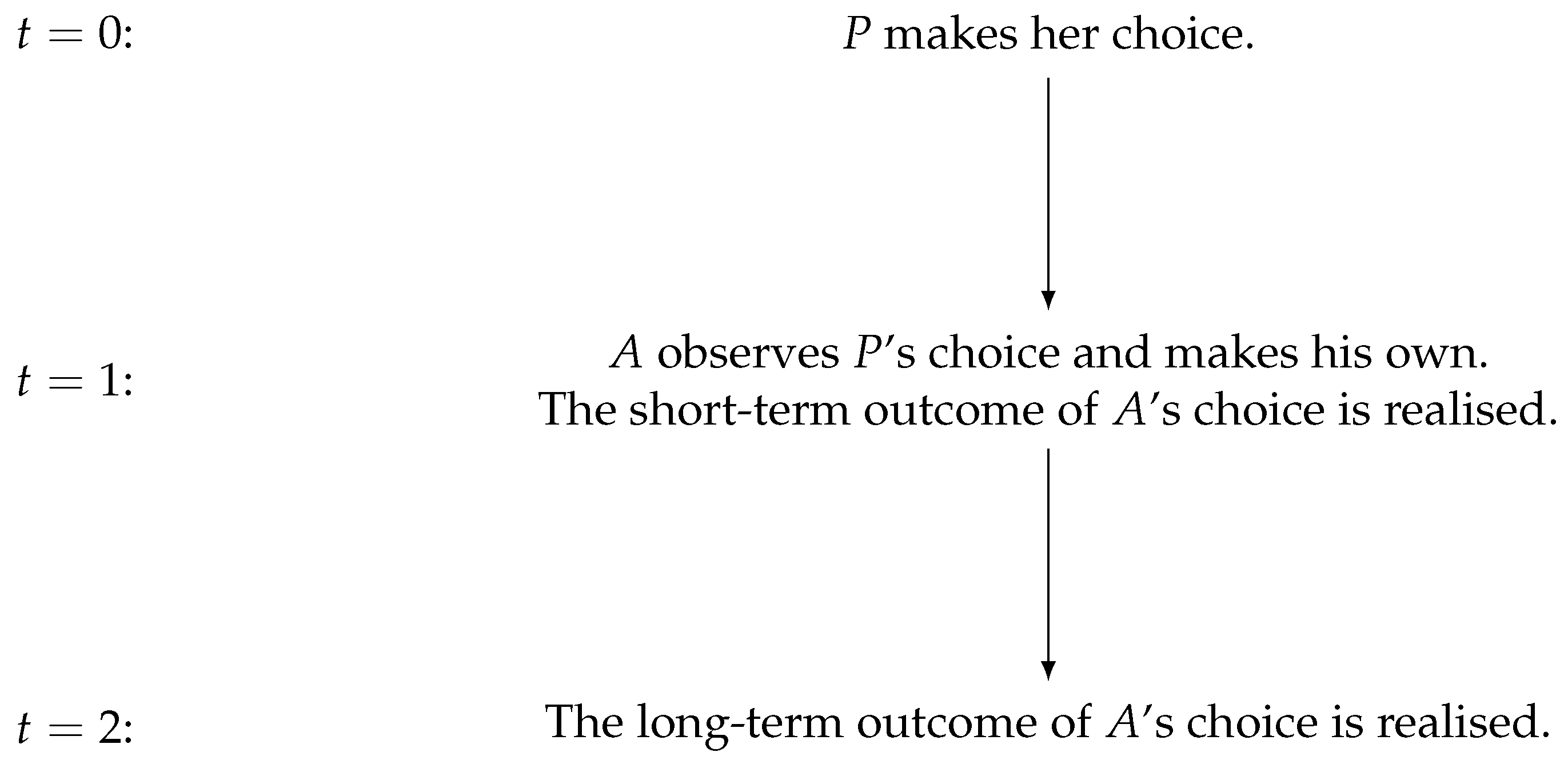
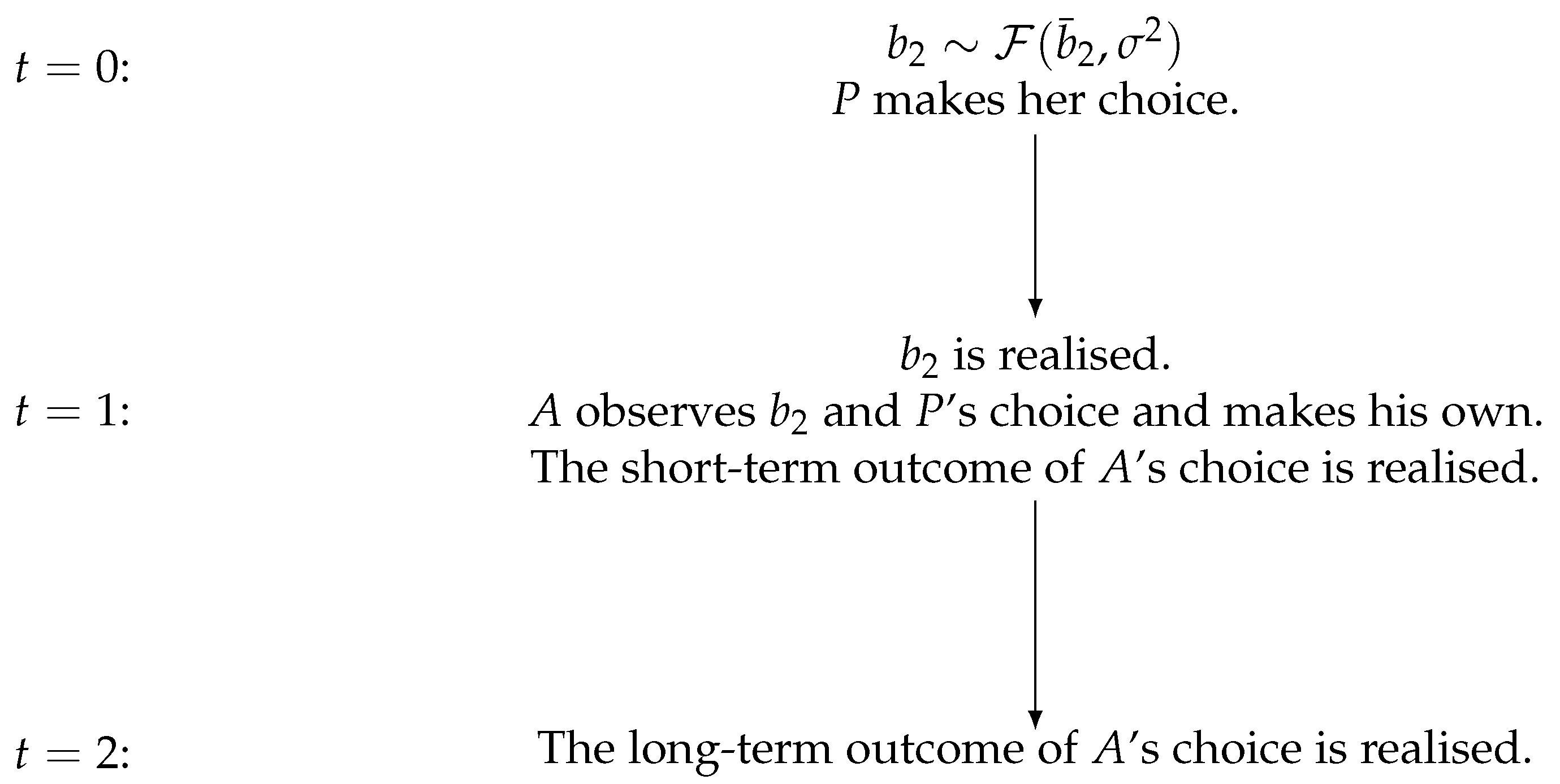
To summarise, in the period , the principal selects so as to maximise the joint utility of herself and the agent, evaluated according to her preferences at that time. The agent observes the principal’s move and subsequently makes his own choice, at , between actions F and B. The agent’s choice yields both a short- and a long-term outcome. The short-term outcome is realised immediately upon his choice, i.e., at . The long-term outcome is realised in the following period, i.e., at . A timeline of the events is provided in Figure 1.
Throughout our analysis, we apply backward induction to solve the game. The principal knows that, at time , the agent will choose, between actions B and F, the one that maximises his utility, as expressed in Equation (2). She therefore knows the outcome of every sub-game that starts with the agent making a choice. Then, at , the principal will choose the value of n that maximises her utility, as expressed in Equation (1) (or (4), see Section 2.3 below), given the agent’s profile of choices. The natural solution concept for this problem is thus the Subgame-Perfect Nash Equilibrium (SPNE).
The fact that the players’ preferences are present-biased can create a conflict of interest. This is because the principal does not internalise fully the agent’s preferences, but instead applies imperfect empathy. That is, she evaluates the agent’s material payoff through the lens of her own preferences at .14 As a result, from the point of view of the principal, the agent appears impulsive. His present bias may lead him to choose action B, whereas he would be better off, in P’s own assessment, were he to opt for F instead. To correct for this bias, given her inability to eliminate it directly, she can opt instead to imbue A with a direct preference for one of the actions.
The inability of the principal to address the present-bias problem of the agent directly is, indeed, critical for our account. At first glance, this might seem arbitrary. Why should the principal not simply invest in eliminating this feature from the agent’s preferences? One argument is that our model would still apply in a situation where the principal could indeed influence , but only to some extent or at too high a cost. A stronger argument can be made about the nature of each source of motivation. In our discussion in Section 1, we have described present bias as an innate characteristic, an impulse similar to the drive for profit. Such an impulse may emerge as an evolutionarily optimal feature of preferences under certain conditions. By contrast, we have described the principal’s intervention as a form of indoctrination. That is, the principal is able to interfere with the agent’s preferences to some extent, but, by instilling a preference for a particular action, rather than eliminating an impulse. It is this distinction that renders our account relevant. As a final point, such constraints are common in this literature (see e.g., [22] on the constraints in information processing).
Equations (1) and (2) highlight the potential for discrepancy between the choice favoured by the principal and the one the agent prefers. To see this, consider the following example, where . Here, P would prefer A to choose B iff:
On the other hand, A will opt for B iff:
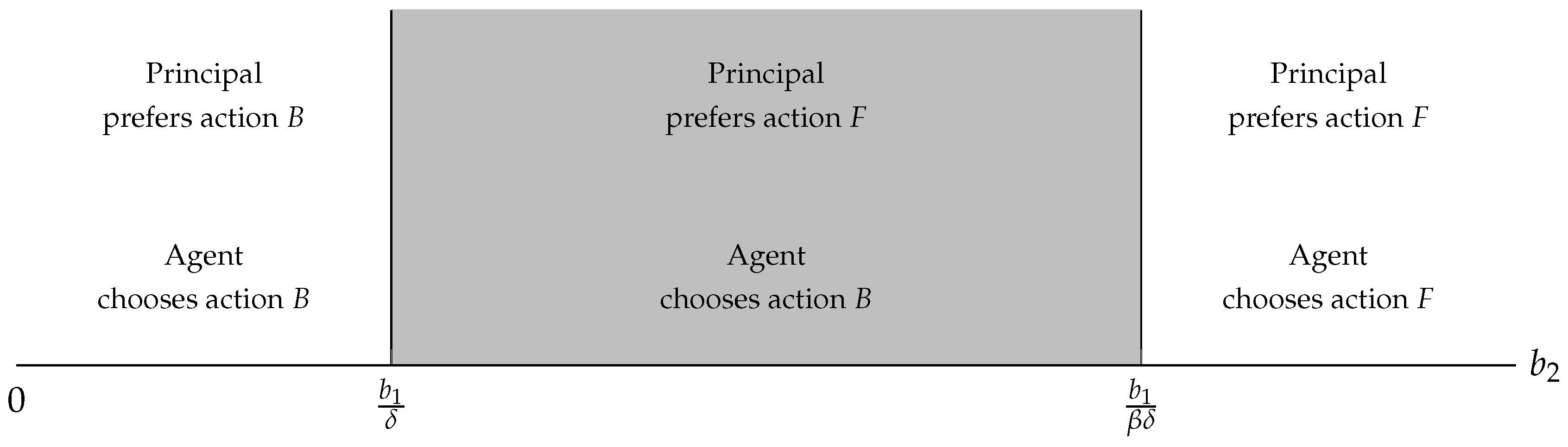
Thus, the agent would switch from B to F at a higher threshold value for . From the point of view of the principal that would be sub-optimal. In simple terms, P would like A to opt for action F so long as the period-1 gain from switching to B falls short of the period-2 cost discounted by . However, A would need a period-2 cost of at least in order to be induced to switch to F. That would render him impulsive in P’s opinion: due to his present-biased preferences, he would assign an unreasonably high weight on his period-1 utility. This situation, where the principal does not interfere with the agent’s preferences at all (), is illustrated in Figure 2.
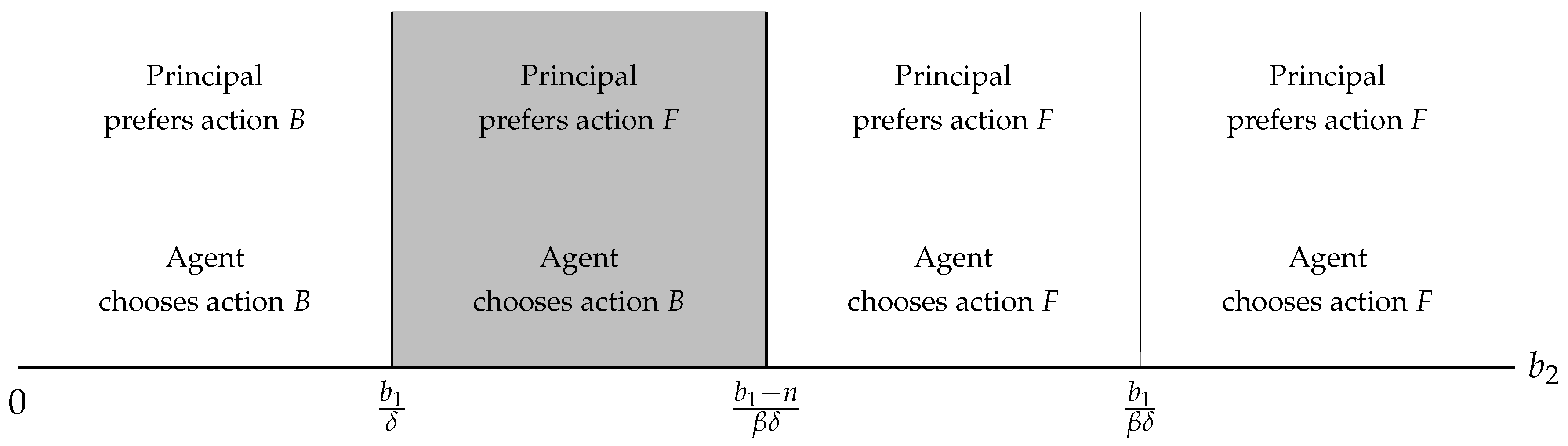
Suppose now that the principal chooses instead to instil a direct preference for action F at , so that . That will induce the agent to lower his threshold for switching from B to F. Recall that n is entirely inconsequential and, thus, of no value to the principal. That is, P chooses to condition A to receive some warm glow from action F that is additional to its material consequences.15 This does not affect the material consequences implied by the choices available to the agent or his present bias, but it does affect his utility. In this way, it counteracts his impulse and brings his preferences closer to those of the principal. The resulting situation looks like the one depicted in Figure 3.
Notice that so far the magnitudes of and are both deterministic, that is, there is no uncertainty associated with any of them. We start from this case, in Section 2.2, because it is useful as a basis for comparison. In Section 2.3, we consider a more realistic scenario, by allowing for uncertainty over .
2.2. Baseline
Some important remarks are in order. To start with, notice that the principal would have no incentive to set , as that would not only be more costly for her, but also counter-productive. Indeed, such a value for n would induce the agent to choose action F even in instances where the principal would want him to opt for B. In addition, the principal would have no incentive to instil a preference for action B instead.16 Doing so would also be counter-productive, as it would increase the discrepancy between the two players’ preferences.
Lastly, it can be easily shown that the sequences of actions in Figure 2 and Figure 3 would be reversed if it was the case that . That is, if action B led to a present cost and a future benefit, then both players would favour F for and both would choose B for . For they would disagree, with the principal favouring B and the agent choosing F. Then, the former would find it optimal to assign to action B. Taking these observations into account, we can form the following proposition.
Proposition 1.
In any equilibrium of game , .
Proof.
Formally, this can be proved by contradiction. Consider first the case where and, thus, P assigns n to action F.
- i.
- Suppose : Then, it would be true that . Thus, A would choose action B and P would have been better off setting .
- ii.
- Suppose : Then, it would be true that . Thus, A would choose action F, even though P would prefer action B. Therefore, P would have been better off setting .
- iii.
- Suppose : For A would choose action F, in line with P’s preferences. If , P would be indifferent between actions F and B, as they would both result in . Setting would render A indifferent between the two actions at a positive cost to P. Thus, P would be better off setting n slightly below , so as to avoid the unnecessary expenditure in the case where .
An equivalent argument holds in the case where and P attaches n on action B. ☐
Proposition 1 describes the upper and lower bound for n. In simple terms, it determines the values of n for which it makes sense for the principal to consider.
Consider now the situation outlined in Section 2.1 from the principal’s perspective at . The principal knows that in period 1 the agent will choose based on:
If the future cost from action B is such, that the preferences of the agent are at odds with those of the principal, then the latter may find it optimal to invest in n. In other words, if , then P may optimally assign on action F, so as to induce A to choose it at . This depends on the cost of doing so. To simplify the analysis, suppose that, when the agent’s preferences render him indifferent between the two options, he always chooses action F. Then, the various different cases are summarised in the following proposition.
Proposition 2.
Given game with , P assigns to action F such, that:
- i.
- if , then and A will choose action F.
- ii.
- if , then and A will choose action B.
- iii.
- if , then
Proof.
The proof of this proposition is straightforward. Trying to maximise their joint welfare, the principal compares the material gain that results from with its cost. When both players agree on which action the agent should take, there is no need for investment in n. When they do not, if , then it is precisely such that it makes the agent indifferent between F and B (given the assumption stated above, that in such cases the agent opts for F). Any higher or lower value would incur an additional cost to the principal with no added benefit. Thus. the principal has to compare what she gets by setting with the cost, , of doing so. If the benefit surpasses the cost, then is set equal to ; otherwise, it is set equal to 0. ☐
The instrumental view of indoctrination championed in our paper gives rise to a rich structure of variations. Recall that the level of n the principal optimally attaches onto an action is dependent on the material consequences implied by that action relative to those implied by the alternative. In our simple scenario, the value of n attached on action F varies with the net benefit/cost of action B. The latter is expressed as a comparison between and , evaluated at . The following corollaries summarize how changes in these two parameters affect .
Corollary 1.
Consider game with and assigned on action F. The relationship between and is non-monotonic. That is, . In particular, an increase in will encourage P to increase the level of at a one-to-one rate, so long as remains lower than . If becomes equal to or greater than , the value of will drop to zero.
Corollary 2.
Consider game with and assigned on action F. The relationship between and is non-monotonic. That is, . In particular, an increase in past will encourage P to decrease at a rate lower than one-to-one (equal to ), unless is already equal to zero. For values lower than or equal to , will be equal to zero.
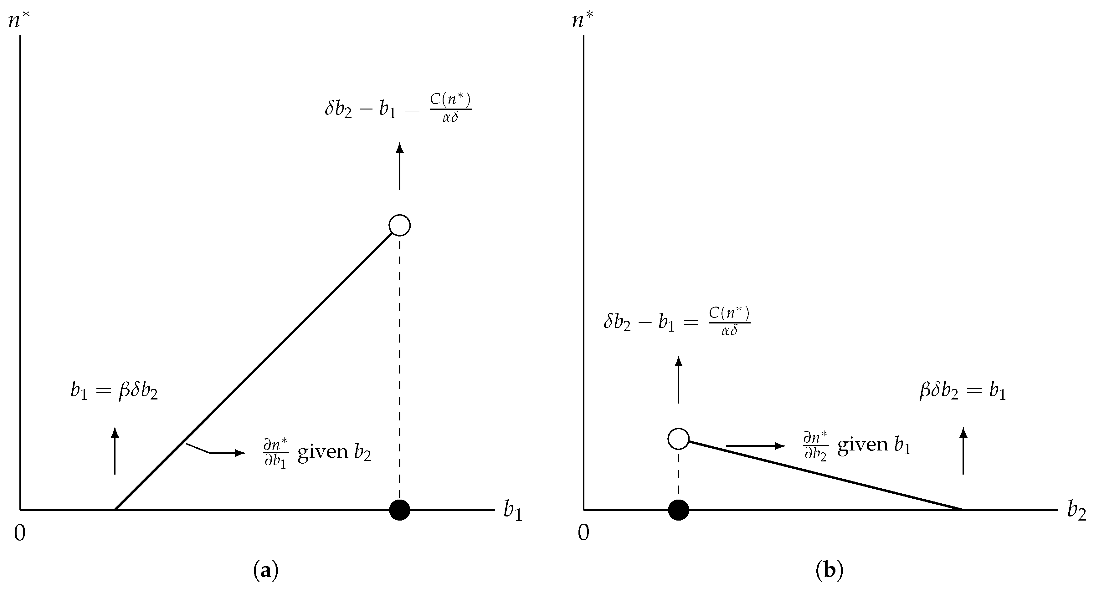
An increase in increases the appeal of action B to the agent. Therefore, if the principal still thinks that opting for it is non-optimal, she will need to invest in a higher level of n to avert it. As increases, there comes a point where such an investment is sub-optimal from the principal’s point of view: what the agent gains by choosing F is not enough to justify the cost of n necessary to induce him to do so. From that point onward, the only sensible option for the principal is to set . A fall in also increases the appeal of action B to the agent. Therefore, again, the principal needs to increase n to ensure that the agent will opt for F. As keeps dwindling, there comes a point where the net material benefit of B does not cover the cost of her investment (as evaluated by the principal). From that point onward, further reductions in will not change n from zero. Figure 4a,b illustrate these two cases.
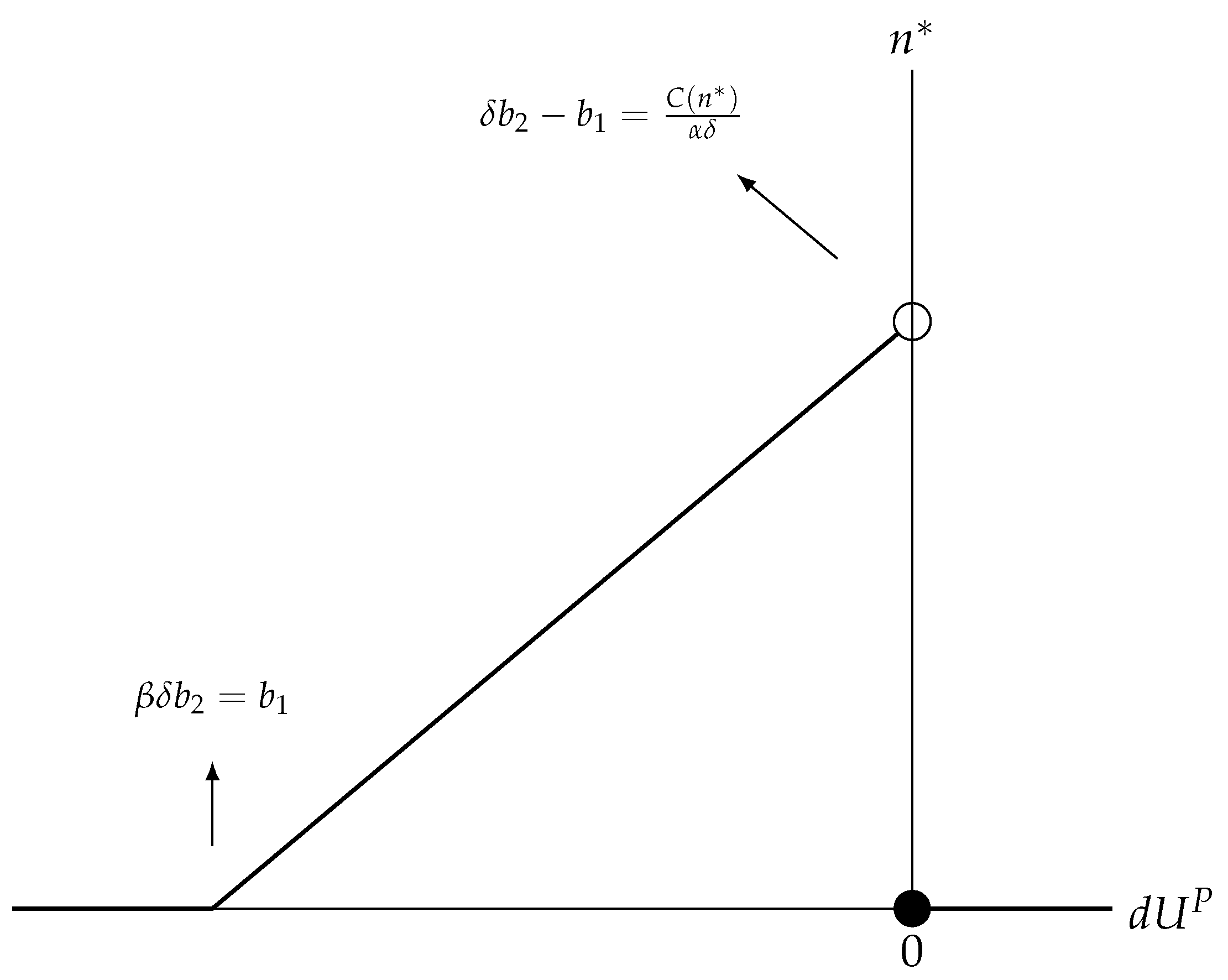
We can describe the variations in , the optimal level of n, as responding to variations in the principal’s total utility. Recall that her utility depends on hers and the agent’s joint material payoff. This, in turn, is determined by her decision on n and the agent’s choice between actions F and B. Based on our previous analysis, the optimal value for n will be either equal to zero or such that will render the agent exactly indifferent between F and B. This is true for any pair of values, and , preference parameters, , , and , and linear cost function, . We can, thus, describe as a function of the difference in P’s utility between the following two combinations of choices:
Figure 5 illustrates how changes in affect . It is worth noting that attains its highest levels in our framework for values close to zero. This is true when the net cost from action B, as evaluated by the principal at , is only marginally higher than the cost of the level of n necessary to avert it. In other words, a relatively high n is necessary when action B is sub-optimal, but only just so.
We now turn to examine the case where the principal does not know ex ante, only that it follows a certain distribution, .
2.3. Probabilistic Future Cost
In this sub-section, we allow for some information asymmetry to arise over the value of , the future consequence of action B. Specifically, the principal is now unaware of the actual value of when she makes her decision. She only knows that it follows a specific distribution, with a positive mean and a certain variance. The agent, on the other hand, knows its exact value when he makes his choice. Suppose that is normally distributed in and let be the cumulative distribution function, with the corresponding probability-density function represented by . Then, the timeline of the events is akin to that in Figure 6.
This new structure enhances the generality of our results. To see this, note that our framework accommodates cases where is ex ante definite as instances where . In addition, in many applications, it is intuitively plausible. Indeed, the principal can be fairly certain about the degree of gratification the agent can expect instantaneously upon making a decision. However, future consequences related to that decision are inherently compromised by environmental volatility-changes in exogenous factors that the principal may not even be aware of, let alone able to influence. In this sense, the agent has an informational advantage simply by being closer to these future consequences. The material payoff of the agent will thus now feature in the principal’s utility in expected terms:
The agent’s utility, on the other hand, is still represented by Equation (2). Taking Equations (2) and (4) into account, the principal’s problem can be stated as follows:
Here, is the agent’s total material payoff across periods 1 and 2. The particular functional form of the distribution of may imply more than one local maxima for Equation (5). To maintain simplicity, we impose two technical assumptions, which jointly ensure that the maximum is unique.
Assumption 1.
Given game , let denote the density function according to which is distributed. Then, is quasi-concave in .
Assumption 2.
In any game , .
Assumption 1 implies that the marginal gain from n will not increase again once it has started decreasing. Given that is increasing in n, a unique maximum point is implied. Assumption 2 precludes the possibility of a minimum occurring before a maximum as n increases. This would be possible if, for example, for n sufficiently small, the cost of increasing it surpassed its additional benefit. Assumptions 1 and 2 together ensure that P’s problem attains a unique optimum solution, which confers the maximum return to n.
Assumptions 1 and 2 are rather restrictive, but their purpose is to maintain the analysis simple. Note that the set of values for that are relevant to P’s problem is bounded by and . Thus, a solution would be attainable even with a different functional form for . The additional complication would be a comparison across all local maxima to determine the global one(s). Moreover, the same would be true even in the presence of local minima. We simply chose to sidestep these additional complexities, in order to refrain from further obscuring our analysis.
Bearing the above in mind, we can now proceed to characterise the solution to P’s problem in the face of uncertainty. Proposition 3 presents this result.
Proposition 3.
Consider game with and in line with Assumptions 1 and 2. Then, the optimal n satisfies:
The proof can be found in Appendix A. The result is, by construction, consistent with the analytical perspective of methodological individualism. That is, n will be assigned a positive value only if it is instrumental to the achievement of P’s goal, and only to the extent that it has a higher rate of return compared to its cost. We thus see that the instrumental character of indoctrination does not change when uncertainty is introduced. The solution to P’s problem is qualitatively similar to the one in our baseline version.
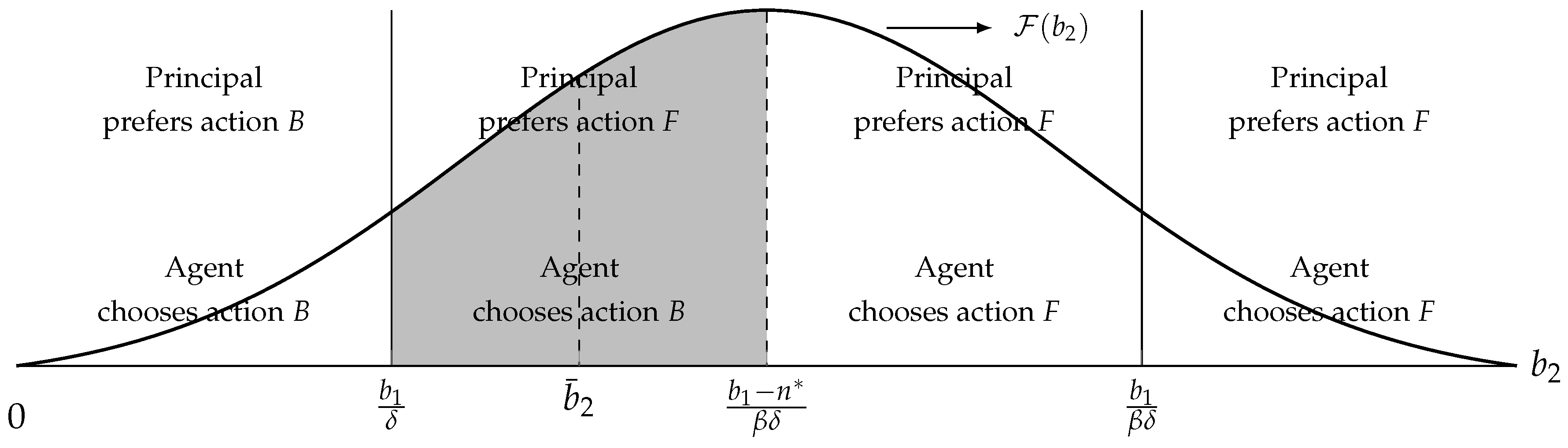
What about the agent’s decision? In our baseline scenario, the value of would be such that he would always be exactly indifferent between actions B and F, and would eventually choose F, in line with the principal’s preference.17 In this new scenario, however, it is possible that the agent’s choice will not reflect the principal’s preference, even given her investment in n. The reason is that the actual realisation of may be so low that he may find it profitable to choose action B even with the additional intrinsic utility n associated with action F. Figure 7 illustrates such a scenario.
Given that the possibility is now open for the agent’s choice to be different from what the principal would want, we can also assess how the probability of this scenario varies with and the distribution of . To do so, we need to formally distinguish between cases where the choice of A agrees with P’s preference and cases where the two differ.
Definition 2.
Compliance: The degree of conformity following P’s choice of is the cumulative probability that A’s choice will agree with P’s preference given .
Using Definitions 1 and 2, we now turn to examine how and compliance are affected by changes in and .
Corollary 3.
Consider game satisfying Assumptions 1 and 2. An increase in the value of , from to may lead to a higher , so long as Assumption A2 remains satisfied. However, compliance may be lower as a result of the increase in .
Proof.
See Appendix B. ☐
Corollary 3 points out that changes in may affect and compliance in different ways. Suppose that increases. This implies that both players will be more inclined to opt for action B than before. However, the discrepancy between their preferences widens. To see this, notice that the agent’s switching threshold changes by a greater margin than the principal’s one does. Therefore, the range of values for which their preferences are conflicting is now larger. As a result, if the principal still prefers action F, then the previous level of is no longer optimal. In particular, the increase in induces her to increase n, in order to account for the additional appeal of action B relative to action F.
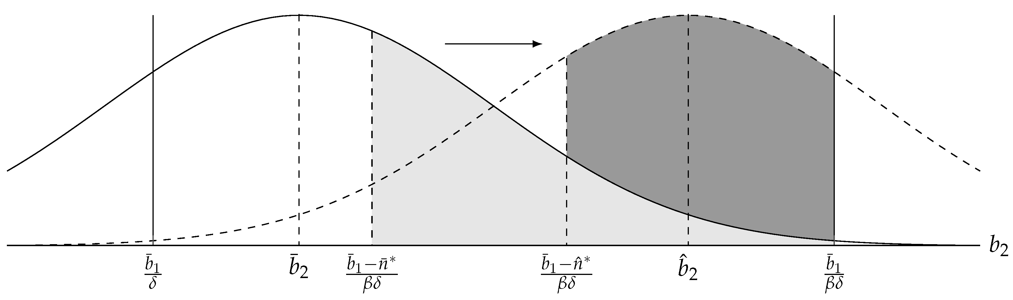
It is important to bear in mind that, in adjusting to account for the change, the principal is interested in its marginal benefit, not what she gets out of it on average. It may well be the case that on average the agent will choose action B, contrary to the principal’s preference. However, it may still make sense for her to invest in n, so long as what she gets from doing so (in expected terms) is more than what she spends on it. Figure 8 illustrates this situation, given a linear cost function and a normal distribution for . In this scenario, an increase in results in a higher and a lower degree of compliance.
The positive relation between and also implies that a decrease in will likely be followed by a reduction in the level of . Intuitively, the change renders option B less appealing and, therefore, encourages the principal to reduce the level of indoctrination, so as to lower its cost. We thus observe a trade-off between the exogenous incentive to opt for the option that the principal favours and the endogenous intrinsic preference she instils herself.
Corollary 4.
Consider game satisfying Assumptions 1 and 2. A parallel rightward shift of , which increases from to , where , may induce P to invest less in n. However, such a shift will always result in greater compliance.
Proof.
See Appendix B. ☐
An increase in the magnitude of the expected future consequence can lead to a lower level of . The intuition behind this result is straightforward. As the increase in renders option B less attractive, the principal will eventually be discouraged from investing in n. The reason is that its instrumentality dwindles. As the agent becomes more likely to avoid B anyway, investing in n and assuming the cost of doing so gets progressively counter-productive.
Thus, the increase in may be partially crowded out by the decrease in the incentive to instil a given level of n. The same trade-off ensues between the agent’s extrinsic and intrinsic incentives to act in a particular way. In the face of higher exogenous motivation, his intrinsic preference dwindles, because it is no longer relevant.
It is worth noting that this is also true when the magnitude of the expected future consequence goes towards the opposite direction. The reasoning is the same as before. A reduction in may induce the principal to compensate by increasing n. However, successive reductions will eventually discourage her from increasing n, as the preference discrepancy becomes progressively less relevant.
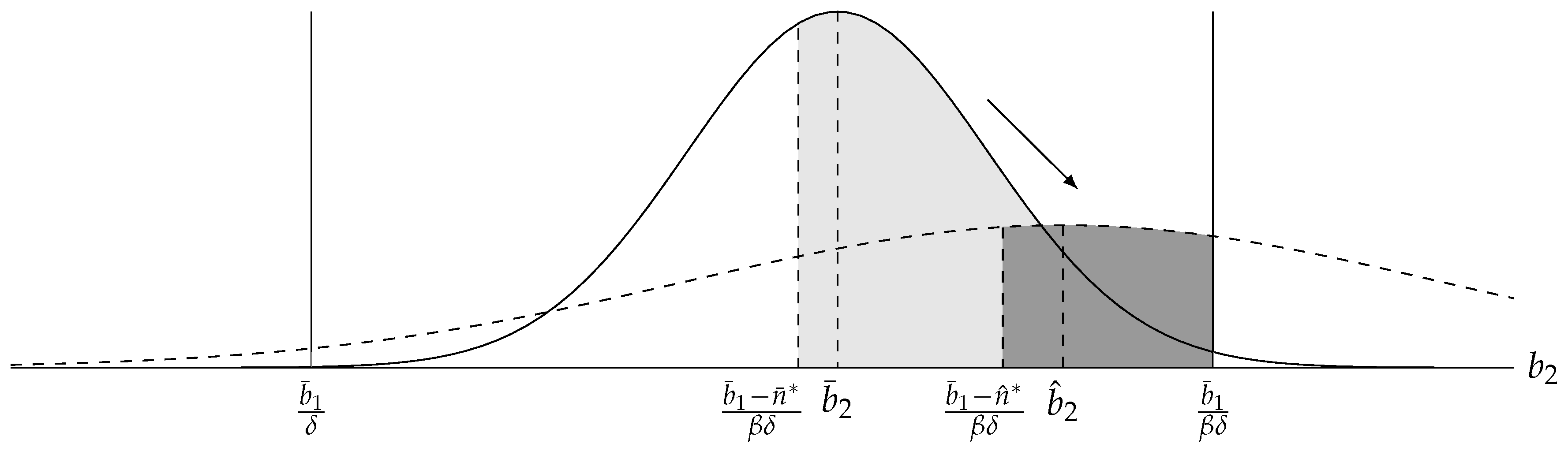
In line with the previous arguments, the agent’s degree of compliance with the principal’s preference depends on the initial distribution of . If in the first place, then any subsequent increase will lead to higher compliance. Figure 9 presents a situation where a higher results in both a lower and a higher degree of compliance.
Notice that the crowding-out of the intrinsic preference by the material cost is always accompanied by enhanced compliance. To see why, consider a situation where the expected cost of action B is such that the principal should optimally assign to action F. If increases, then the principal will only settle for a lower level of n if it confers a greater return than the previous one. Investing in n is not more expensive than it was before. If anything, she could still invest in it to the extent she did before. If she chooses to undercut her investment, it is because this is the optimal response.
Notice that Corollary 4 describes a variance-preserving shift. That is, it refers to a change in the distribution of to a higher expected value, but with the same degree of uncertainty. This is important for our analysis, as our conclusion that the increase in always results in an increased degree of compliance does not necessarily hold if we allow for simultaneous changes in its variance. To see this, consider a situation where an exogenous shift affects both and . Since is affected by both, the effects of this change may actually counteract each other. We explore this possibility in the following Proposition.
Proposition 4.
Consider game satisfying Assumptions 1 and 2. Suppose that an exogenous shock changes the distribution of to one that has a higher mean and a higher variance. Such a shock may induce P to invest less in n and may also lead to a lower degree of compliance.
Proof.
See Appendix C for a proof by example. ☐
Proposition 4 highlights the potential conflict between two effects that result from the distributional change. One of these effects comes as a result of the higher expected future consequence. The other follows from the increased uncertainty about that consequence. The net effect on and the degree of compliance can be surprising.
As it has already been argued (see Corollary 4), an increase in may reduce the principal’s incentive to invest in n. However, the principal’s incentive is crowded out due to the fact that, given the new even a lower n makes the agent more likely to comply (by choosing action F). Thus, the increase in (given ) leads to a higher degree of compliance.
The increase in , on the other hand, may induce to fall even further. This is because, as the future consequence becomes more volatile, the marginal return that the principal receives by increasing n gets progressively lower. Intuitively, the increased uncertainty implies that the most likely values are now less probable. As a result, it becomes difficult for the principal to pinpoint a level for n that is highly likely to be optimal.18 Given that the cost of providing n has not changed, the principal may find it better to reduce n in response to higher uncertainty.
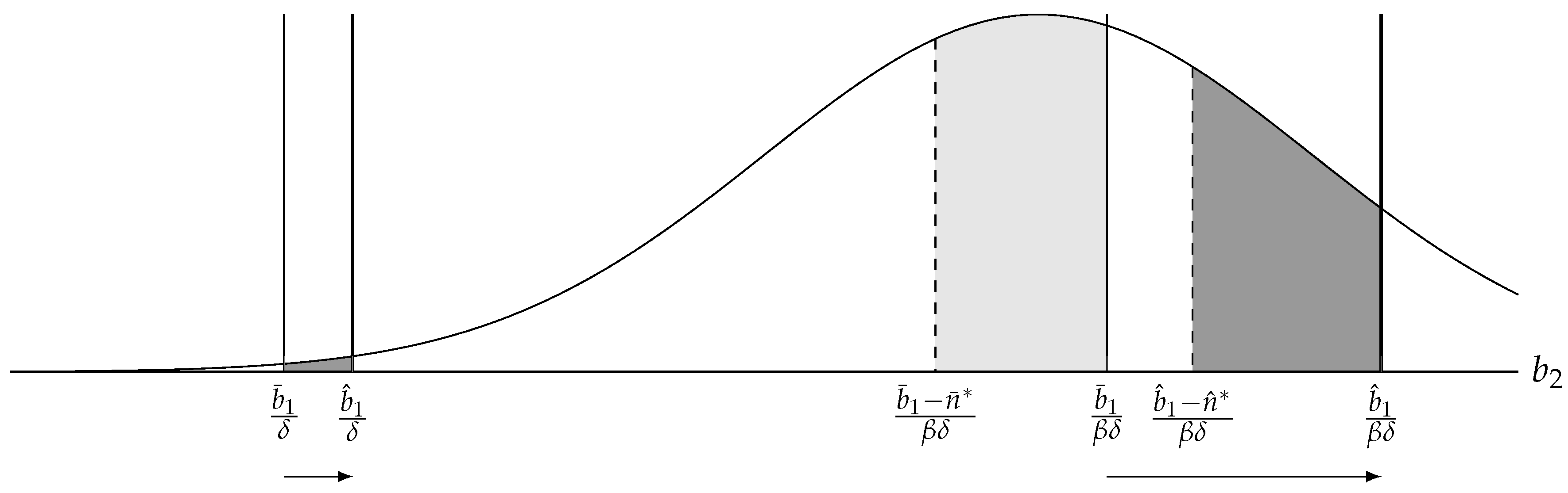
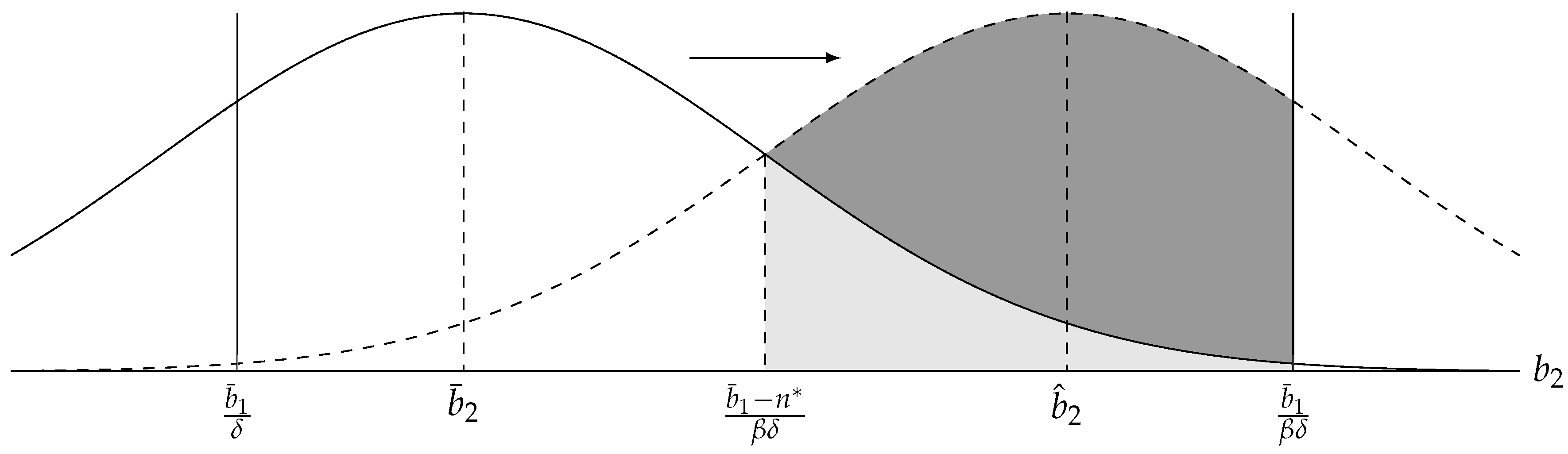
The final outcome may, thus, resemble the one illustrated in Figure 10. This is a case where a shift towards a higher but more volatile results in a reduced probability of the agent choosing in accordance with the principal’s preference. Consequently, apart from crowding out n, the change also renders the agent more vulnerable to present bias. This result is all the more striking when considered in light of the intuition that a higher on its own would have the exact opposite effect.
We have thus far examined the changes in and the degree of compliance induced by changes in and the distribution of . As a final remark, we note that varies monotonically with , to which it is inversely related. That is, other things being equal, an increase in the marginal cost of instilling n always leads to a lower level for the intrinsic preference and vice versa. In particular, there is no crowding-out related to the principal’s incentives: a reduction in will render her unambiguously more willing to provide a higher . The same is true with respect to compliance.
3. Discussion
This section explores some of the potential applications of our framework. It discusses firstly some implications for public policy, where the government can be viewed as the principal and a representative citizen as the agent. It then examines cultural transmission under a parent–child interpretation. It concludes with a discussion of self-control problems as viewed from the perspective of the intertemporal self. Note that the examples reported below are not exhaustive. The domain of application of our theory is much more general and includes all instances where one-shot decisions can have consequences at multiple points in time.19
3.1. Public Policy
We turn to some consequences of our analysis for the design of public policy. Our aim is to demonstrate that, owing to the strategic interplay analysed in Section 2, the results of policy measures may be very different from those originally expected. To do so, we use examples of policies that may prove inefficient, given the policymaker’s stated goals.
Consider, thus, a policy aimed at encouraging more people to save some of their income, e.g., an increase in the interest rate, taking effect at . Such a policy will have an effect on the amount of period-2 consumption one has to forfeit in order to spend more money in period 1. In the context of our model, it amounts to an exogenous increase in . Should we expect that this policy will be successful, and to what extent? One factor that may limit the policy’s effectiveness is the change in the culture of parsimony that its announcement initiates. As Corollary 4 points out, a greater may crowd out private and public investment in promoting frugality. Thus, even in the absence of additional effects stemming from the announcement of the policy, the resulting increase in the proportion of savers may not be as high as initially expected.
Suppose, now, that the government aims to discourage tax avoidance while in the midst of an austerity programme. To do so, it imposes stronger sanctions to perpetrators. However, owing to the need for austerity, it is also required to cut back on audits. What does the resulting situation look like? The announcement of stricter penalties (higher ) is set to increase compliance, although it is also expected to discourage a culture of duty to pay one’s taxes (lower n). The reduction in oversight, however, results in these penalties being more unlikely than before. As a result, it mitigates both the sense of social responsibility and compliance. Proposition 4 suggests that the resulting effect on taxes may well be negative.
Lastly, consider a policy that aims to reduce carbon emissions. One way of doing so would be to collect research on the adverse consequences for the environment and, thus, the society’s future prospects. Then, this research would be disseminated, perhaps in the form of short advertisements, in a bid to increase environmental awareness among the population. Our analysis shows that there may be a caveat in this reasoning. Specifically, if the research appears inconclusive, so that many possible future scenarios seem likely but none is deemed particularly probable, the policy may backfire. Furthermore, as Proposition 4 points out, this can be true even if the additional information results in the situation appearing more dire on average. Thus, our framework suggests that caution must be exercised in the release of information as part of a policy measure.
The three examples outlined above highlight the trade-off between people’s (exogenous) material incentives and their (endogenous) intrinsic motivation. By providing extrinsic incentives, public policies may end up crowding out intrinsic motivation. In doing so, they are compromising, at least partly, their own effects (this result is consistent with [30], among others). Our analysis indicates that caution needs to be exercised when assessing the potential effects of a proposed policy measure.
3.2. Cultural Transmission
The transmission of cultural values across generations has traditionally been modelled by means of dynamic games played by successive agents. In constructing such a process, Ref. [10] applies the imperfect-empathy setup of [11]. The result is a model of parent–child interaction. The assumptions made are that (a) parents can affect the deep preferences of their children and (b) parents try to maximise a notion of utility of their children that departs from pure material welfare. This general framework of parent–child interaction (with alternatives to imperfect empathy) is becoming increasingly popular as a means of explaining social dynamics and cultural change.20
In this interpretation, the principal in our model can assume the role of the parent, while the agent that of the child. It is then straightforward to see how parental indoctrination can be modelled as a principal–agent game, where the former takes an interest in the utility of the latter. Notice that, in the parent–child interpretation, it is not necessary that the players suffer from present bias, only that the agent’s discount factor is different than that of the principal.
3.3. Self Control
We can also evaluate the scope of our framework through the perspective of the intertemporal self (in the spirit of [46]). To this end, consider a game that is being played among the various instances of the same person, acting at different points in time. It is natural to assume that in this case . Then, our analysis focuses on the action of her self at and the choice of her self at . Suppose that this person is initially characterised solely by preferences over outcomes and that she also exhibits present bias. Suppose, further, in line with the previous setup, that, while she knows about her bias, she cannot eliminate it per se. Then, in trying to maximise her intertemporal utility, she might optimally set .
How can such a result be interpreted? From the point of view of the self, at it is (weakly) optimal to commit to preferring an action over another. She knows that, if she is equipped only with materialistic preferences, then it is probable that, in the face of temptation, she will make an ill-preferred choice. To reduce this probability, she may want to commit to a particular code of conduct, so as to enhance the appeal of the alternative option.
An appealing feature of this account of preference formation is its general applicability. Note that the aforementioned code of conduct can be grounded on various premises, such as moral principles (see [47,48]), social norms (see [49,50]), reputation (see [51,52,53,54]), and habitual or conventional decision-making (see [55,56,57], as well as [58]).21 All such concerns can be shown to be instrumental from a purely materialist viewpoint. Thus, such preferences can also emerge through an evolutionary process, assuming that present bias is also at play (through a reasoning similar to [22]).
4. Conclusions
We propose a game-theoretic model of endogenous preference formation, where an action-based inclination is optimally chosen to counterbalance present-biased proclivities. We build on the idea that preferences are, to some extent, malleable. We then investigate the relationship between material incentives and intrinsic motivation. Our analysis indicates that the relationship between the two is non-monotonic. Our results are especially relevant to the domain of policy analysis.
The theory presented here describes how the endowment of an intrinsic preference can be optimal from a materialistically rational perspective. We depict the dialectics between parameter variations and individual incentives and show how the effects of the former can sometimes crowd out the latter. These effects are important, both with respect to cultural transmission and to the exercise of self-control. The effectiveness of a policy is demonstrated to depend, at least to some extent, on it providing the right mix of incentives to individuals.
The paper does not consider the intergenerational dynamics that ensue in such a context. This is a fascinating research question in its own right. Here, instead, we propose two main arguments: that preferences for actions can be rationally assigned and that they should be taken into account when considering the effects of changes in the underlying economic environment.
Funding
This research received no external funding.
Acknowledgments
The author is grateful to Silvia Sonderegger and Daniele Nosenzo for their unwavering support and invaluable guidance, as well as to two anonymous referees for their thoughtful comments. The financial support provided by the Economic and Social Research Council (ESRC) is gratefully acknowledged.
Conflicts of Interest
The author declares no conflicts of interest.
Appendix A. P’s Problem
Consider the objective function of P as defined by Expression (5). Upon satisfaction of the first-order condition:
The second-order condition for a strict maximum suggests that:
Appendix B. Parameter Variations
We now investigate how variations in the parameters of the model affect the level of n and the rate of A’s adherence to P’s preference. We focus firstly on . Recall that according to Equation (A1):
Deriving (A3) with respect to , we find:
Consider an exogenous shift from to , where . Let and . Note that P will respond to the change in by adjusting n according to (A3). Therefore, (A4) and (A5) together add up to:
Thus, it is true that:
The sign of depends on the sign and magnitude of . To see this, recall firstly that inequality (A2) implies that has a lower bound:
This means that the denominator of the fraction on the right-hand side of Equation (A6) is positive for every that constitutes a maximum (assuming that ). The numerator, on the other hand, will be negative if:
Taking the above into account, we can discern the following cases:
It is worth noting that, when , will fall to zero following an increase in . The reason is that, from Assumption 2, it can be seen that is decreasing more rapidly than . Thus, as is the case in our baseline scenario, in response to an increase in P will either increase , or eliminate it altogether. We can describe the relationship between changes in and changes in in a general proposition. Consider game with , , and . Suppose that is replaced with , where . Such a change will, ceteris paribus, lead to:
- , if ,
- , if ,
- , if .
The first of these cases corresponds to Corollary 3. It suggests that, so long as the percentage change in the frequency of the cut-off point is above a certain threshold, P will have an incentive to increase in response to increases in .
Changes in also have a bearing on compliance, which, according to Corollary 3, may be negative. Following our definition of compliance (2), we can measure its variations as changes in the cumulative probability that A’s choice wil not conform with P’s preference. As this probability dwindles, the degree of compliance increases.
Let be the cumulative probability that the choice of A will be different from P’s preference. Then, , where is the cumulative distribution function of distribution . Consider, then, the change in this difference in response to a change in :
Given that (from Equation (A6)), the first term of the right-hand side of (A8) is always positive. Therefore, for a sufficiently low , an increase in will lead to a lower degree of compliance.
To clarify this argument further, we also provide a numerical example. Consider game with , , , , , , and , where is the normal distribution with mean , variance , and probability density function . Let be the equilibrium level of n corresponding to and the one corresponding to . Then, from Equation (A1), solving for :
Solving out, we obtain approximately equal to 1. On the other hand, solving for :
Again, solving out, we obtain approximately equal to 2.875. We see that P has increased in response to the rise in . With respect to compliance, it is easy to see that the cumulative probability of disagreement between the two players has increased. In particular, under , this probability is equal to:
Under , on the other hand, it becomes:
Thus, compliance decreases following the increase of from to .
We now turn to variations in and their effect on . In what follows, . In accordance with Assumptions 1 and 2, let , where is quasi-concave. To start with, suppose that a variance-preserving shift occurs, from to , where . In other words, the distribution shifts towards higher values of , making option B less appealing than before. Let denote the equilibrium n under and that under . In addition, let denote the probability density function of distribution and that of distribution . It is straightforward to verify from Equation (A3) that an increase (decrease) of the density of the cut-off point that has resulted from a change in the distribution will lead to an increase (decrease) in . The reason is that such a change adjusts the importance of in the determination of . In other words, it is true that if , then , while if , then . In addition, from (A3), the following two equations are true:
Therefore, it follows that:
Then, comparing with , one can see that:
The converse is also true:
Suppose, now, that , that is, that the cost function is weakly convex in n. In this case, and vice versa. Thus:
It thus becomes apparent that Equation (A11) implies an upper and a lower bound for the density of the new cut-off point, . That is, the density of a cut-off point that has resulted from an increase in n can never be lower than that of the initial cut-off point. Conversely, the density of a cut-off point that has resulted from a reduction in n will never surpass that of the initial cut-off point. This result implies that a parallel (variance-preserving) shift in the distribution of , such as the one described above, always enhances compliance.
To see why this is the case, consider such a change, whereby rule is replaced by such, that , where . Recall that is the equilibrium level of n under and that under . Then, it is true that:
To see this, one can start from and show that this is, in fact, not equal to .22 Recall that, if was an equilibrium level under , then it would need to satisfy (A3). However:
It is obvious that (A3) is not satisfied by . Therefore, P has an incentive to further increase n, thereby increasing the probability that A will make her preferred choice in the next period.
We can organise our findings with respect to variance-preserving distributional shifts in another general proposition. Consider game with , , and . Consider a shift from to , where . Let denote the probabilty density function of distribution and denote the probability density function of distribution . Then, such a change will, ceteris paribus, lead to:
- , if ,
- , if ,
- , if .
If, additionally, , then, ceteris paribus, the probability that A’s choice will comply with P’s preference increases as grows larger (as in Figure A1).
Figure A1.
: The expected future consequence is relatively larger, but the level of is the same.

Appendix C. Example of a Distributional Shift
What if both the mean and the variance of increase as a result of the distributional shift? This is the case pertaining to Proposition 4, which states that such a change may decrease both and compliance. We show how this can be the case through an example situation. Consider game with , , , , , , and , where is the normal distribution with mean , variance , and probability density function . Let be the equilibrium level of n under distribution and that is under . Then, from Equation (A1), solving for :
Solving out, we obtain approximately equal to 1.38. On the other hand, solving for :
Again, solving out, we obtain approximately equal to 0.67. Thus, the level of has decreased as a result of the distributional shift. Regarding compliance, let denote the cumulative distribution function of . Then, under the share of values for which A would conform with P’s preference in the case of conflict was:
Under the share of values for which A will conform with P’s preference in the case of conflict becomes:
Thus, both and compliance decrease as a result of the distributional shift. The results are illustrated in Figure 10, in Section 2.3. In general terms, the proposition may be stated as follows. Consider game with , , and . Consider a shift from to , where and . Let denote the probability density function of distribution and denote the probability density function of distribution . Then, such that and the degree of compliance is lower.
References
- Hobbes, T. De Cive (The Citizen); Appleton-Century-Crofts: New York, NY, USA, 1949. [Google Scholar]
- Stigler, G.J.; Becker, G.S. De gustibus non est disputandum. Am. Econ. Rev. 1977, 67, 76–90. [Google Scholar] [CrossRef]
- Adriani, F.; Sonderegger, S. Why do parents socialize their children to behave pro-socially? An information-based theory. J. Public Econ. 2009, 93, 1119–1124. [Google Scholar] [CrossRef] [Green Version]
- Algan, Y.; Cahuc, P.; Shleifer, A. Teaching Practices and Social Capital; Technical Report; National Bureau of Economic Research: Cambridge, MA, USA, 2011. [Google Scholar]
- Acemoglu, D.; Jackson, M.O. History, Expectations, and Leadership in the Evolution of Social Norms; Technical Report; National Bureau of Economic Research: Cambridge, MA, USA, 2011. [Google Scholar]
- Bowles, S. Endogenous preferences: The cultural consequences of markets and other economic institutions. J. Econ. Lit. 1998, 36, 75–111. [Google Scholar]
- Laffont, J.J.; Martimort, D. The Theory of Incentives: The Principal-Agent Model; Princeton University Press: Princeton, NJ, USA, 2009. [Google Scholar]
- Prendergast, C. The provision of incentives in firms. J. Econ. Lit. 1999, 37, 7–63. [Google Scholar] [CrossRef]
- Edmans, A.; Gabaix, X. Executive compensation: A modern primer. J. Econ. Lit. 2016, 54, 1232–1287. [Google Scholar] [CrossRef]
- Tabellini, G. The scope of cooperation: Values and incentives. Q. J. Econ. 2008, 123, 905–950. [Google Scholar] [CrossRef]
- Bisin, A.; Verdier, T. The economics of cultural transmission and the dynamics of preferences. J. Econ. Theory 2001, 97, 298–319. [Google Scholar] [CrossRef]
- Ainslie, G. Specious Reward: A Behavioral Theory of Impulsiveness and Impulse Control. Psychol. Bull. 1975, 82, 463–496. [Google Scholar] [CrossRef] [PubMed]
- Ainslie, G. Picoeconomics: The Strategic Interaction of Successive Motivational States within the Person; Cambridge University Press: Cambridge, UK, 1992. [Google Scholar]
- Meier, S.; Sprenger, C. Present-biased preferences and credit card borrowing. Am. Econ. J. Appl. Econ. 2010, 2, 193–210. [Google Scholar] [CrossRef]
- Benhabib, J.; Bisin, A.; Schotter, A. Present-bias, quasi-hyperbolic discounting, and fixed costs. Games Econ. Behav. 2010, 69, 205–223. [Google Scholar] [CrossRef] [Green Version]
- Laibson, D. Golden eggs and hyperbolic discounting. Q. J. Econ. 1997, 112, 443–477. [Google Scholar] [CrossRef]
- O’Donoghue, T.; Rabin, M. Doing It Now or Later. Am. Econ. Rev. 1999, 89, 103–124. [Google Scholar] [CrossRef]
- Gul, F.; Pesendorfer, W. Temptation and Self-Control. Econometrica 2001, 69, 1403–1435. [Google Scholar] [CrossRef] [Green Version]
- Bénabou, R.; Tirole, J. Self-confidence and personal motivation. Q. J. Econ. 2002, 117, 871–915. [Google Scholar] [CrossRef]
- Bénabou, R. The economics of motivated beliefs. Rev. Econ. Polit. 2015, 125, 665–685. [Google Scholar] [CrossRef]
- Bénabou, R.; Tirole, J. Mindful economics: The production, consumption, and value of beliefs. J. Econ. Perspect. 2016, 30, 141–164. [Google Scholar] [CrossRef]
- Samuelson, L.; Swinkels, J. Information, evolution and utility. Theor. Econ. 2006, 1, 119–142. [Google Scholar]
- Becker, G.S. A theory of social interactions. J. Polit. Econ. 1974, 82, 1063–1093. [Google Scholar] [CrossRef]
- Phelps, E.S. Altruism, Morality, and Economic Theory; Russell Sage Foundation: New York, NY, USA, 1975. [Google Scholar]
- Cornes, R.; Sandler, T. Easy riders, joint production, and public goods. Econ. J. 1984, 94, 580–598. [Google Scholar] [CrossRef]
- Cornes, R.; Sandler, T. The Theory of Externalities, Public Goods, and Club Goods; Cambridge University Press: Cambridge, UK, 1996. [Google Scholar]
- Steinberg, R. Voluntary donations and public expenditures in a federalist system. Am. Econ. Rev. 1987, 77, 24–36. [Google Scholar]
- Andreoni, J. Impure altruism and donations to public goods: A theory of warm-glow giving. Econ. J. 1990, 100, 464–477. [Google Scholar] [CrossRef]
- Varvarigos, D. Cultural norms, the persistence of tax evasion, and economic growth. Econ. Theory 2017, 63, 961–995. [Google Scholar] [CrossRef]
- Bohnet, I.; Frey, B.S.; Huck, S. More order with less law: On contract enforcement, trust, and crowding. Am. Polit. Sci. Rev. 2001, 95, 131–144. [Google Scholar] [CrossRef]
- Lindbeck, A.; Nyberg, S. Raising children to work hard: Altruism, work norms, and social insurance. Q. J. Econ. 2006, 121, 1473–1503. [Google Scholar]
- Adriani, F.; Sonderegger, S. Signaling about norms: Socialization under strategic uncertainty. Scand. J. Econ. 2018, 120, 685–716. [Google Scholar] [CrossRef]
- Adriani, F.; Sonderegger, S. The Signaling Value of Punishing Norm-Breakers and Rewarding Norm-Followers. Unpublished work. 2018. [Google Scholar]
- Lizzeri, A.; Siniscalchi, M. Parental Guidance and Supervised Learning; Technical Report, Discussion Paper; Center for Mathematical Studies in Economics and Management Science: Evanston, IL, USA, 2006. [Google Scholar]
- Doepke, M.; Zilibotti, F. Occupational Choice and the Spirit of Capitalism; Technical Report; National Bureau of Economic Research: Cambridge, MA, USA, 2007. [Google Scholar]
- Doepke, M.; Zilibotti, F. Parenting with Style: Altruism and Paternalism in Intergenerational Preference Transmission; Technical Report; Forschungsinstitut zur Zukunft der Arbeit: Bonn, Germany, 2012. [Google Scholar]
- Cosconati, M. Parenting Style and the Development of Human Capital in Children; Job Market Paper; University of Pennsylvania: Philadelphia, PA, USA, 2009. [Google Scholar]
- Bhatt, V.; Ogaki, M. Tough Love and Intergenerational Altruism. Int. Econ. Rev. 2012, 53, 791–814. [Google Scholar] [CrossRef]
- Bernheim, B.D.; Shleifer, A.; Summers, L.H. The strategic bequest motive. J. Polit. Econ. 1985, 93, 1045–1076. [Google Scholar] [CrossRef]
- Lindbeck, A.; Weibull, J.W. Intergenerational aspects of public transfers, borrowing and debt. Scand. J. Econ. 1986, 88, 239–267. [Google Scholar] [CrossRef]
- Wilhelm, M.O. Bequest behavior and the effect of heirs’ earnings: Testing the altruistic model of bequests. Am. Econ. Rev. 1996, 86, 874–892. [Google Scholar]
- Pinker, S. The Blank Slate: The Modern Denial of Human Nature; Penguin: London, UK, 2003. [Google Scholar]
- Turkheimer, E. Three laws of behavior genetics and what they mean. Curr. Dir. Psychol. Sci. 2000, 9, 160–164. [Google Scholar] [CrossRef]
- Heckman, J.J.; Stixrud, J.; Urzua, S. The Effects of Cognitive and Noncognitive Abilities on Labor Market Outcomes and Social Behavior; Technical Report; National Bureau of Economic Research: Cambridge, MA, USA, 2006. [Google Scholar]
- Cappelen, A.W.; List, J.A.; Samek, A.; Tungodden, B. The Effect of Early Education on Social Preferences; Working Paper 22898; National Bureau of Economic Research: Cambridge, MA, USA, 2016. [Google Scholar]
- Fudenberg, D.; Levine, D.K. A Dual-Self Model of Impulse Control. Am. Econ. Rev. 2006, 96, 1449–1476. [Google Scholar] [CrossRef] [PubMed] [Green Version]
- Alger, I.; Weibull, J.W. A generalisation of Hamilton’s rule: Love others how much? J. Theor. Biol. 2012, 299, 42–54. [Google Scholar] [CrossRef] [PubMed]
- Alger, I.; Weibull, J.W. Homo Moralis—Preference Evolution under Incomplete Information and Assortative Matching. Econometrica 2013, 81, 2269–2302. [Google Scholar]
- Bicchieri, C. The Grammar of Society: The Nature and Dynamics of Social Norms; Cambridge University Press: Cambridge, UK, 2006. [Google Scholar]
- Bicchieri, C. Norms, Preferences, and Conditional Behavior. Pol. Phil. Econ. 2010, 9, 297–313. [Google Scholar] [CrossRef]
- Binmore, K. Game theory and the social contract. In Game Equilibrium Models II; Springer Nature: Berlin, Germany, 1991; pp. 85–163. [Google Scholar]
- Binmore, K. Natural Justice; Oxford University Press: Oxford, UK, 2005. [Google Scholar]
- Binmore, K. Why do people cooperate? Pol. Phil. Econ. 2006, 5, 81–96. [Google Scholar]
- Gächter, S.; Falk, A. Reputation and Reciprocity: Consequences for the Labour Relation. Scand. J. Econ. 2002, 104, 1–26. [Google Scholar] [CrossRef] [Green Version]
- Lewis, D.K. Convention: A Philosophical Study; Blackwell Publishers: Hoboken, NJ, USA, 1969. [Google Scholar]
- Sugden, R. Spontaneous Order. J. Econ. Perspect. 1989, 3, 85–97. [Google Scholar] [CrossRef] [Green Version]
- Sugden, R. Thinking as a Team: Towards an Explanation of Nonselfish Behavior. Soc. Philos. Pol. 1993, 10, 69–89. [Google Scholar] [CrossRef]
- Binmore, K. Social norms or social preferences? Mind 2010, 9, 139–157. [Google Scholar] [CrossRef]
- Binmore, K. Modeling Rational Players: Part I. Econ. Philos. 1987, 3, 179–214. [Google Scholar] [CrossRef]
- Binmore, K. Modeling Rational Players: Part II. Econ. Philos. 1988, 4, 9–55. [Google Scholar] [CrossRef]
- Binmore, K. Do conventions need to be common knowledge? Topoi 2008, 27, 17–27. [Google Scholar] [CrossRef]
- Elster, J. Social Norms and Economic Theory. J. Econ. Perspect. 1989, 3, 99–117. [Google Scholar] [CrossRef] [Green Version]
- Paternotte, C.; Grose, J. Social Norms and Game Theory: Harmony or Discord? Br. J. Philos. Sci. 2012, 64, 551–587. [Google Scholar] [CrossRef]
| 1. | |
| 2. | |
| 3. | In our framework both individuals exhibit present-biased preferences, but it is the present bias of the agent that is incentivising the principal. |
| 4. | Present bias also has a theoretical rationale as a feature of humans’ preferences in an evolutionary sense. If the information reception and processing mechanisms of humans are imperfect (as in the context of [22]), then their uncertainty about the environment may induce them to place a lot of weight on present consumption. |
| 5. | It is interesting to note that the principal has such an incentive even though she exhibits present bias herself. |
| 6. | We are grateful to an anonymous referee for pointing out several such instances. |
| 7. | The two players may very well be different temporal versions of the same agent (i.e., the same person at different time-periods), but in general this need not be the case. |
| 8. | This is without loss of generality. Given any and in some , where is the material-payoff function of agent A in period , subtracting from both will not alter A’s decision. |
| 9. | The same relationship could have been achieved by restricting both and to be negative. Indeed, the important element is that they are of the same sign. Consider this alternative case, where a present loss is weighted against a future benefit. It is straightforward to show that this scenario is a reflection of ours. Owing to the symmetric structure of the analysis, our results are invariant across the two. |
| 10. | |
| 11. | This interpretation is relevant to situations where the action space for A contains more than two distinct elements, which we will not examine here. Indeed, due to the associated cost, when two actions are available to agent A, attaching some value of n to one of them only is optimal. |
| 12. | Indeed, is assumed weakly convex for our proofs in Appendix A and Appendix B. |
| 13. | We say that the players exhibit quasi-hyperbolic, time-inconsistent preferences. |
| 14. | The general principle of imperfect empathy is quite standard in the principal–agent literature (see [11]). |
| 15. | Notice that in our characterisation the degree of intrinsic utility assigned to an action is dependent on its material consequences. The level of n is chosen by the principal in order to account for the agent’s present bias and not because she believes that it has any real value. One way to think about this instrumentalist approach would be to consider that P can assign n to virtually any action available to A, so long as, given the underlying parameter values, she prefers it more than he does. Note, however, that for A this additional value is meaningful, in the sense that his utility increases by n whenever he performs the associated action. |
| 16. | In this paper, we focus on positive values for n in an effort to determine the action that will be chosen, as opposed to that which will be avoided. The two are equivalent in our framework, where the agent faces a binary-choice problem. However, in a situation with three or more available actions, assigning a negative n to an action (aversion towards a certain type of behaviour) does not generally ensure that the desired action will be chosen. A comparison between the cost of discouraging certain types of behaviour and that of encouraging others is an interesting research project itself. We leave this for the future and focus instead on positive education (encouragement of a particular behaviour). |
| 17. | The same would be true in expected terms, if the cost of action B was uncertain for both players. So long as P and A had the same distribution of in mind, A’s choice would be anticipated by P: They would both form the same expectation about . Thus, even if the actual value of eventually proved to be different than what they had expected, their choices would coincide. |
| 18. | Recall that the optimal level of n would render the agent exactly indifferent between options B and F. |
| 19. | In fact, our paper is relevant to an even wider class of studies. Consider, for example, the model proposed by [29], where practices of tax evasion, as soon as they have been established, are perpetuated as history-dependent cultural norms. Our paper can be seen as complementary to his, due to the fact that we focus on the mechanism by which cultural indoctrination takes place across generations. |
| 20. | |
| 21. | |
| 22. | If it were, the cut-off point would be in the same relative position given with that of under . |
Figure 1.
Timeline of events.

Figure 2.
, no preference for a particular action.

Figure 3.
assigned on action F.

Figure 4.
(a) relationship between and given and : so long as there is a conflict of preferences between P and A and the cost of indoctrination is sufficiently low, n increases in ; (b) relationship between and given and : given that there is conflict of preferences between P and A and the cost of indoctrination is sufficiently low, n decreases in .

Figure 5.
Relationship between and : Indoctrination is at its highest when its net benefit is only marginal.
Figure 5.
Relationship between and : Indoctrination is at its highest when its net benefit is only marginal.

Figure 6.
Timeline of events— uncertain at .

Figure 7.
Misalignment of preferences: Here, P has optimally assigned on action F knowing that is drawn from , but the realised value, , induces A to opt for action B. The shaded area is the cumulative probability of all such values.
Figure 7.
Misalignment of preferences: Here, P has optimally assigned on action F knowing that is drawn from , but the realised value, , induces A to opt for action B. The shaded area is the cumulative probability of all such values.

Figure 8.
: The immediate consequence from option B is relatively larger and so is the level of . The proportion of values for which A’s choice will conform with P’s preference is now lower.
Figure 8.
: The immediate consequence from option B is relatively larger and so is the level of . The proportion of values for which A’s choice will conform with P’s preference is now lower.

Figure 9.
: The expected future consequence is larger, the level of is lower, and the probability of compliance is higher.
Figure 9.
: The expected future consequence is larger, the level of is lower, and the probability of compliance is higher.

Figure 10.
: The expected future consequence is larger and more uncertain. The level of and the degree of compliance are both lower.
Figure 10.
: The expected future consequence is larger and more uncertain. The level of and the degree of compliance are both lower.

© 2018 by the author. Licensee MDPI, Basel, Switzerland. This article is an open access article distributed under the terms and conditions of the Creative Commons Attribution (CC BY) license (http://creativecommons.org/licenses/by/4.0/).
Share and Cite
MDPI and ACS Style
Kotsidis, V. Call to Action: Intrinsic Motives and Material Interests. Games 2018, 9, 92. https://0-doi-org.brum.beds.ac.uk/10.3390/g9040092
AMA Style
Kotsidis V. Call to Action: Intrinsic Motives and Material Interests. Games. 2018; 9(4):92. https://0-doi-org.brum.beds.ac.uk/10.3390/g9040092
Chicago/Turabian StyleKotsidis, Vasileios. 2018. "Call to Action: Intrinsic Motives and Material Interests" Games 9, no. 4: 92. https://0-doi-org.brum.beds.ac.uk/10.3390/g9040092
Note that from the first issue of 2016, this journal uses article numbers instead of page numbers. See further details here.