Article

Factor Analysis of XRF and XRPD Data on the Example of the Rocks of the Kontozero Carbonatite Complex (NW Russia). Part II: Geological Interpretation

1
Geological Institute, Kola Science Centre, Russian Academy of Sciences, 14, Fersmana Street, 184209 Apatity, Russia
2
South Urals Federal Research Center of Mineralogy and Geoecology of the Urals Branch of the Russian Academy of Sciences, Ilmen Nature Reserve, 456317 Miass, Russia
*
Author to whom correspondence should be addressed.
Submission received: 27 August 2020 / Revised: 20 September 2020 / Accepted: 22 September 2020 / Published: 26 September 2020
(This article belongs to the Special Issue Multivariate Analysis Applications to Crystallography)

Abstract

:
Numerical comparison of mineralogical and geochemical data, which is required in a variety of geological applications, is a challenging task, especially when analyzing extensive sample collections. Herein, we apply factor analysis (FA) to a collection of 198 diffraction patterns of bulk rock samples from the Kontozero carbonatite complex. The mineralogical information hidden in the X-ray powder diffraction (XRPD) data is thereby squeezed down to a set of two dozen variables represented by factor scores (FS). The values of these FSs show a functional relationship with the contents of the minerals composing the rocks. Therefore, factor scores can be considered as a beneficial tool for rapid qualitative and semiquantitative analysis of the mineral composition of rocks. Supplementing principal component analysis (PCA) with FSs as independent variables characterizing the mineral content of rocks allows for the numerical comparison of mineralogical and geochemical data. By PCA, we reveal the main trends in the mineralogical and geochemical evolution of the investigated rocks of the Kontozero complex. Furthermore, the results are obtained in the very first stages of the research. This fact elucidates the potential use of the proposed technique in geological studies and mining.

1. Introduction

Three methods are capable of providing accurate determinations of the mineralogical phase composition: (1) point-counting techniques using optical microscopy (optical modal analysis), supplemented by image digitalization and analysis and the application of electron microscopy techniques; (2) modal X-ray powder diffraction (XRPD); (3) normative calculation from bulk chemical data. Reviews and comparisons of these and related methods have been published in many articles; for example, see [1,2,3]. Though highly advantageous, each method has limitations. Optical modal analysis, which has long been successfully used in geology [4,5], has two significant drawbacks: (a) it is time-consuming, and (b) it yields mineralogical information only about a small section of the rock (samples for research are usually sub-inch size). Some progress has been made in solving the first problem thanks to electron microscopy techniques and their automation [6,7,8,9,10,11]. The latter fact becomes a problem when studying heterogeneous rocks. Modal XRPD and normative calculation are used to investigate bulk rock powders and, therefore, can provide data on a significant amount of rock. Of these, the first method is considered a powerful approach [12,13]. However, when studying rocks with complex mineral composition, the overlapping of peaks challenges the task. In this case, prior knowledge about the set of mineral phases is critical. Normative calculation (e.g., CIPW and similar techniques [14,15,16]) is rapid, but requires an adequate calculation algorithm to obtain correct results. This algorithm should consider both the mineral composition of rocks and the chemical specificity of the constituent minerals of variable composition (e.g., feldspars, micas, pyroxenes, and so on).
For a small sample of rocks (up to several tens of samples), it is preferable to use a combination of all three methods. They effectively complement each other, which guarantees a good result [3]. When processing extensive collections of samples—for example, when exploring deposits—the assessment of mineral contents by the uniform application of all three methods becomes a laborious task. Faced with this problem, researchers prefer normative calculation from bulk chemical data using statistical data processing as the least labor-intensive technique [1,2]. Optical modal analysis and modal X-ray powder diffraction are often used to verify the results. However, as noted above, the development of a calculation algorithm for normative calculations is not always possible.
We encountered these problems when studying the alkaline–carbonatite volcanic–plutonic Kontozero complex. Geological information of the studied part of the complex is scarce. The reports and published materials for Kontozero contain only a rough description of the mineral composition of these rocks and no data on the composition of the minerals. Traditional calculation techniques (e.g., CIPW [16]) have proven to be ineffective and may give utterly incorrect results. As we found, the reason for this is the specificity of the mineral composition of these rocks; namely, the presence of several minerals with equal proportions of all cations, except for silica. Examples are the analcime–natrolite–albite series and the monticellite–diopside pair. At the same time, quartz is often abundant. Furthermore, the rocks contain many phases of variable composition (e.g., Ca–Mg–Fe carbonates and minerals of the pyroxene, amphibole, and mica groups).
The complex mineral composition of Kontozero rocks does not allow for the use of a single algorithm for normative calculation throughout the entire sample set, which consists of almost 200 samples. In this regard, we applied an original technique based on the statistical processing of XRPD data using factor analysis [17]. Like modal XRPD, this technique deals with data of the bulk sample (i.e., on a significant volume of rock). Furthermore, it is a blind method and, therefore, does not require prior mineralogical information. On the contrary, this information results from applying the technique in the form of factors which are readily amenable to mineralogical interpretation. This paper reports on the use of scores of these factors as a tool for the semiquantitative analysis of mineral composition. We also exemplify how the factor scores used as supplementary variables in the statistical study of XRF data allow for mineralogical explanation of the identified geochemical trends.

2. Materials and Methods

2.1. Samples Description

The investigated rock collection comprises 198 core samples from the Kontozero volcano–plutonic alkaline–carbonatite paleovolcanic complex. Kontozero is one of the complexes of the Devonian Kola Alkaline Province [18,19], dating from an age of about 360–380 Ma [20]. This complex is a paleocaldera filled mainly with Kontozero formation rocks (Figure 1) and is surrounded by Precambrian gneisses. According to the data reported by [21,22,23,24,25,26], the Kontozero sedimentary–volcanic formation consists of three units: (1) the upper carbonate–terrigenous (carbonatite) sequence (up to 1000 m thick), which combines carbonatite lavas and tuffs, tuffites, and tuffaceous breccias; (2) the middle volcanogenic (melilitite) sequence (up to 800 m thick) consists of alkali picrite, melanephelinite, nephelinite, phonolite, and tephrite (lavas, lava breccias, and tuffs); (3) the lower terrigenous–volcanogenic (augitite) sequence (up to 750 m thick) is composed of augitite and limbourgite lavas, tuffs, and tuffites with conglomerate and siltstone interbed. Several intrusions of pyroxenites and syenites (alkaline and nepheline) occur on the periphery of the caldera. The central part of the caldera includes a carbonatite–picrite explosion tube and adjacent carbonatite agglomerate tuffs and tuffaceous breccias of vent facies.
Samples from two parts of the Kontozero section were selected for this study. We examined the upper part of the carbonatite–picrite explosion pipe using the drill core #7 (an interval from 4.5 to 293.0 m) and the lower part of the carbonatite sequence using the drill core #6 (an interval from 496.0 to 925.0 m). The core sampling step averaged about 4 m.

2.2. Analytical Techniques

The primary source of information on the mineral composition was X-ray powder diffraction (XRPD) from bulk rock samples. The chemical composition of each sample was determined by X-ray fluorescence analysis (XRF).
X-ray powder diffraction data of the bulk rock samples were collected at room temperature using a Shimadzu XRPD-6000 diffractometer (Shimadzu Corp., Kyoto, Japan), using a Cu target X-ray generator with graphite monochromator. The scan range of the Bragg angle (2θ) was from 4.00° to 70.00°. The work was performed on the analytical equipment of the Institute of Mineralogy UB RAS (Miass, Russia; [27]).
X-ray fluorescence data of the bulk rock samples were collected using the wavelength dispersive X-ray fluorescence spectrometer S4 Pioneer (Bruker AXS, Germany). Instrumental operation conditions for the main rock-forming (Na, Mg, Al, Si, P, K, Ca, Ti, Mn, and Fe) and some minor (Ba, Sr, and Zr) elements were as follows: 30 kV at 80 mA for NaKα, MgKα, AlKα, SiKα, PKα, KKα, and CaKα analytical lines; 50 kV at 40 mA for TiKα, MnKα, FeKα, SrKα, BaKα, ZrKα, and RhKα lines (RhKα Compton line was used as background standard for Sr and Zr determination). Spectral overlaps and matrix effects were calculated by the Fundamental Parameters Method. For the same purpose, we calculated the Sr and Zr contents using the intensity of the incoherent (Compton) anode emission (Rh) scatter peak. The XRF analysis technique used, including estimates of measurement errors, has been detailed in [28]. The research was performed using the equipment of the Joint-use Center “Isotope-geochemical Research” of A.P. Vinogradov Institute of Geochemistry SB RAS (Irkutsk, Russia; [29]).
Raw XRPD and XRF data are listed in Supplementary Tables S1 and S2, respectively.

2.3. Data Processing

This work is based on the results of the factor analysis of XRPD and XRF data for Kontozero rocks, carried out according to the method described in [17]. XRPD data were also the basis for semiquantitative phase analysis, performed using the QualX v. 2.24 program (Institute of Crystallography (IC)-CNR, Bari, Italy; [30,31]), and quantitative phase analysis, conducted using the MAUD v. 2.94 program (University of Trento, Trento, Italy; [32,33]). In both cases, the XRPD database POW_COD [34] was used. The classical FA for geochemical variables (from XRF data) in the modification of the principal component analysis (PCA) was performed using the Statistica v. 12.0 software (StatSoft, Tulsa, OK, USA).

3. Results and Discussion

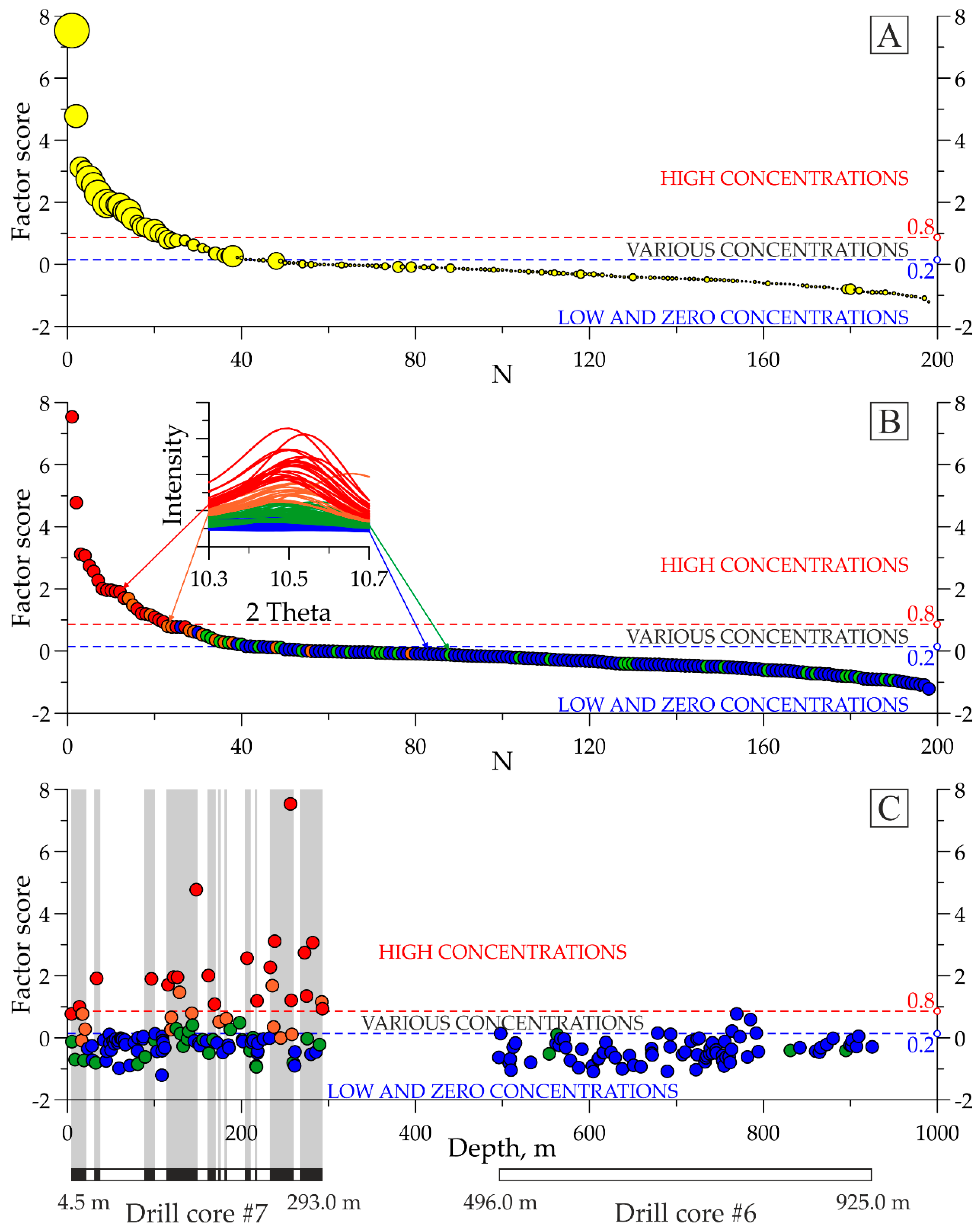
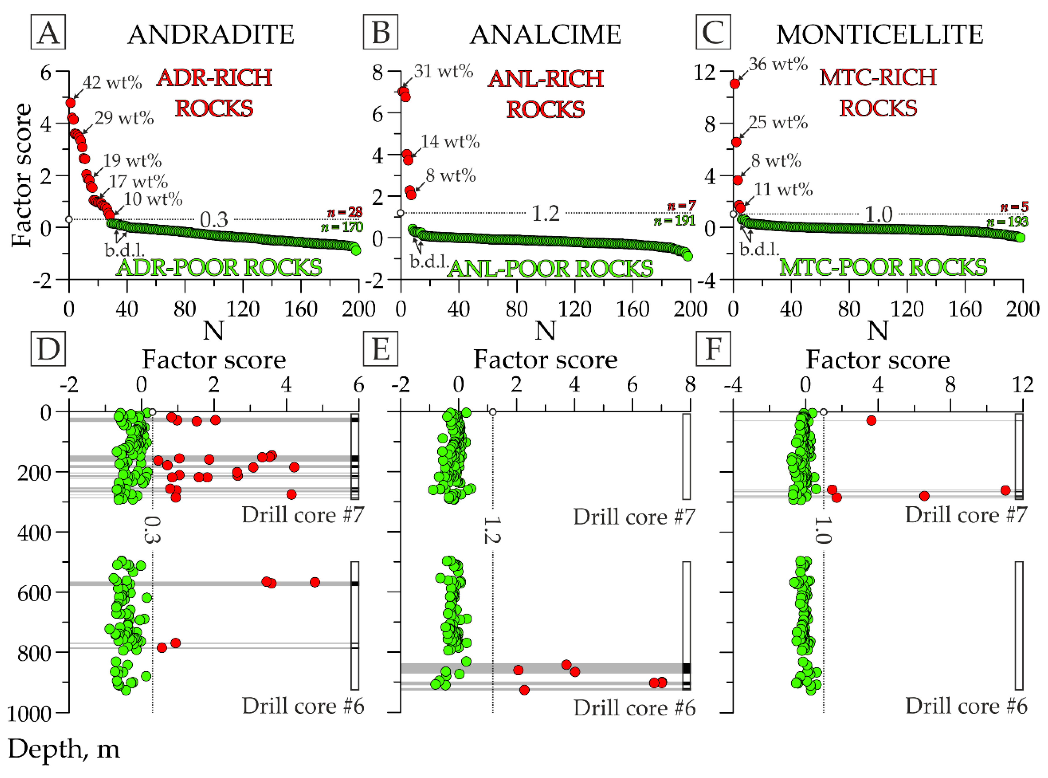
3.1. Use of Factor Scores for Qualitative and Semiquantitative Mineralogical Analysis

XRPD and XRF data of the investigated Kontozero rock sample collection were statistically processed by factor analysis, according to the method described in [17]. The FA extracted many factors, more than 20 of which were interpretable [35]. They corresponded to the following minerals: Ca–Mg–Fe carbonates (calcite, ferruginous dolomite, and siderite), strontianite, burbankite, feldspars (orthoclase and albite), garnet (andradite), monticellite, diopside, biotite, chlorite, serpentine, zeolites (natrolite and analcime), quartz, magnetite, ilmenite, fluorite, fluorapatite, pyrite, and anatase. Petrographic and mineralogical studies have confirmed that all these minerals were present in the tested rocks. Note that some extracted factors corresponded to several minerals simultaneously; for example, factor #7 combined diopside and magnetite. Following the results of FA, we characterized each sample by a set of several dozen new “mineralogical” variables corresponding to the listed minerals. These variables were the factor scores (FS), which describe the magnitudes of factors (factor scores are given in Supplementary Table S3).
To determine how the FS values were related to the mineral contents, we performed the following procedure. The CIF files of the above-listed minerals were selected in the XRPD data COD database [34] (see Appendix A). For this, using the QualX program [31], we chose the standards closest to the mineral phases of Kontozero rocks, both in terms of peak positions and intensity. A working database compiled from these CIF files served as the basis for semiquantitative analysis of the mineral composition of all samples in the QualX program, in which the semiquantitative analysis is based on the reference intensity ratio (RIR; see [36] and the references therein).
Factors that received a mineralogical interpretation showed a functional relationship between FSs and the estimated contents of minerals corresponding to the factors (Figure 2). As noted above, several mineral phases were sometimes associated to the same factor. In such cases, the functional relationship was established between the FS of this factor and each associated phase (see, e.g., Figure 2C,D).
A linear trend satisfactorily described these functional relationships (blue lines in Figure 3). However, the best quality approximation was guaranteed by a polynomial model expressing the relationship between the estimated content of a mineral (x) and the FS of the factor corresponding to this mineral (y) using an equation of the form y = Ax2 + Bx + C, where A, B, and C are constants (red lines in Figure 3).
This relationship validates the mineralogical interpretation of the factors. Moreover, it makes the FS a reliable tool for assessing the content of a mineral corresponding to a factor. Let us show this using the example of calcite: a polynomial trend describes the relationship between the calcite content and the FS of the factor corresponding to calcite (Figure 3A). Nevertheless, the graphs of the calcite content variations (in the range from 0 to 100 wt%) in the studied drill cores and the FS of the calcite factor (in the range from −1 to 3) were similar (Figure 4A,B). Other factors showed similarities between the plots of FS values and the contents of the corresponding minerals. The transition from the FS to the content of a mineral differed in scale between factors. Thus, for semiquantitative analysis using FS, it is sufficient to determine the content of a mineral in samples with the highest and lowest FS values by an alternative method and interpolate.
For many geological tasks, qualitative assessment of mineral content (like high/low content of a phase or its presence/absence) is often sufficient. For example, these are the requirements for the selection of samples rich in (or devoid of) any mineral for specialized mineralogical, geochemical, and isotopic studies. Qualitative information on the mineral composition is also necessary for quantitative analysis. For example, the Rietveld method [37,38] requires prior knowledge of the phase composition for a multicomponent mineral mixture. A rapid estimate of mineral composition can be performed by analyzing the ranked range of FSs (i.e., a graph of FS values arranged in descending order; see Figure 4C). For all factors, the morphology of such graphs is similar: (1) an area of high FS values with a steep slope; (2) an inflection area; (3) an area of low FS values in the form of a linear, subhorizontal plateau. The graphs of some factors (including calcite; see Figure 4C) have smooth inflection, while others show a break at this point. The first type of inflection is characteristic of the factors of the most common minerals, which are abundant in many tens of samples. The second type is common for minerals that are essential in only a small number of probes (from 2–3 to 20–25 samples).
The ranked range of the FS values for alkaline amphibole also had a smooth inflection (Figure 5A,B). A comparison of this graph with the results of the semiquantitative analysis (see Figure 5A) showed that the figurative points of samples with high content of this mineral fell within the region of high FS values (with a steep slope). The segment of low FS values, shaping a subhorizontal plateau, was formed by figurative points of samples in which the content of amphibole was either low or zero. The inflection segment was mainly composed of points of samples rich in amphibole. The positions of samples rich and poor in amphibole intersperse only within a small region near the point of transition to the plateau. Taking into account the significant error in the determination of the mineral content by the RIR method, we made an alternative estimate of the alkaline amphibole content. The diffraction patterns of the studied samples exhibited a pronounced peak for amphibole in the 2θ region from 10.4° to 10.6° (Figure 5B, inset), which was not overlapped by the neighboring lines of other minerals. We collated all diffraction patterns on a single scale of intensity values and compared the maximum peak with the intensities of other peaks in this region. This analysis divided the diffraction patterns and the corresponding samples into four groups:
  • GROUP I represents the samples/diffraction patterns with peak intensity in the considered region above half the maximum peak for the studied sample set (in Figure 5B,C, fragments of the diffraction patterns and the figurative points of the samples included in this group are red-colored);
  • GROUP II has peak intensities from a quarter to half of the maximum peak height (in Figure 5B,C, the elements related to this group are orange-colored);
  • GROUP III has a peak intensity of less than a quarter of the maximum peak height (in Figure 5B,C, the elements related to this group are green-colored);
  • GROUP IV has no peaks in the considered area (in Figure 5B,C, the details concerning this group are blue-colored).
Given this separation, we analyzed the graph of the ranked range of FSs (see Figure 5B). The results of this analysis were entirely consistent with the above comparison between the ranked range of FS and semiquantitative grade. Thus, we reliably documented two boundary values of the FSs: 0.8 (all samples of rocks with a higher FS are rich in amphibole) and 0.2 (most samples with a lower FS do not contain amphibole). Only in a narrow FS range between these values (i.e., just before the graph reaches the subhorizontal plateau) was a “zone of uncertainty” observed. The possibility of the presence of such a zone must be taken into consideration when carrying out a qualitative analysis.
With this in mind, we sorted the samples by FSs in the sections of the studied cores. It was found that the drill core #7 (explosion pipe) contained several intervals, about 30 m in thickness, composed of amphibole-rich rocks; while the drill core #6 (carbonatite sequence) did not contain these rocks at all. Subsequent petrographic and mineralogical studies fully confirmed these results.
Let us show the distribution of FSs for several other mineral phases (Figure 6). The graphs of the FS-ranked range for andradite, analcime, and monticellite factors (as well as all other factors), in contrast to those for calcite and amphibole, had a turning-point inflection.
For control purposes, we selectively calculated the mineral content in some samples from both before and after inflection points (see Figure 6A–C). Quantitative phase analysis was performed in the MAUD program [33] using the Rietveld full-pattern fitting method (see [40] and the references therein). In this analysis, the same CIF files were used as those in the semiquantitative calculations. To the left of the inflection were the points of samples rich in the considered minerals. The right-side points reflected those samples where the content of these minerals was below the detection limit. In this way, an individual FS threshold was traced for each phase. All samples above this threshold were abundant in the mineral in question, relative to other samples in the collection. Thus, the qualitative analysis using the graphs of FS-ranked range with such turning-points is simple. The content of the listed minerals in “rich” samples varied within 10–40 wt%. The situation was different with other minerals; for example, analysis of the burbankite factor showed about 10 samples rich in this phase, but the quantitative analysis counted no more than 2–3 wt% burbankite in them.
Analysis of FS distribution in cores showed that rocks with different dominant minerals occupied different positions in the structure of the Kontozero complex. Rocks abundant in some common minerals, such as calcite, dolomite, and andradite, were found to be ubiquitous (see Figure 4 and Figure 6D). Some minerals were abundant only in the explosion pipe, outcropped by drill hole #7 (e.g., amphibole; see Figure 5C). Rock varieties rich in other minerals (e.g., orthoclase and/or albite) occurred only in the carbonatite sequence, as outcropped by drill hole #6. The third group of minerals (e.g., fluorite and analcime discussed above; see Figure 6E) reached high concentrations in local intervals, composing cement of brecciated rock sections. Some minerals, such as monticellite, were essential only in sparse samples (see Figure 6F).
Thus, the graphs of the FS-ranked range allow for an express qualitative analysis and visualization of mineral distribution in the structure of the studied geological object.

3.2. The Application of Factor Scores for Mineralogical Interpretation of Geochemical Data

The discovered relationship between mineral contents and the scores of the corresponding factors allowed us to form a mineralogical interpretation of the results of the FA, based on geochemical variables (hereafter called “classical FA”; Figure 7A,B).
Classical FA traditionally pursues two goals [41]: (a) classification of observations (in our case, rock samples); (b) searching for correlations between variables (in our case, the contents of elements in rocks). As applied to the chemistry of Kontozero rocks, the classical FA with the modification of principal component analysis (PCA) has shown effectiveness in achieving both goals; for instance, when projecting Factors I and II onto the factor-plane, according to the explained dispersion (48% and 17%, respectively), all points were divided into three groups connected by mutual transitions (Figure 7A).
The positive pole of Factor I explains the group 1 cluster of points (the green field in Figure 7A). Three geochemical variables—namely L.O.I., Ca, and Sr—were associated with this pole (Figure 7B). These variables showed high factor loadings (note: the factor loading is the correlation coefficient between the factor and the original variable, which varies from −1 to 1): FILCa = 0.98, FILL.O.I. = 0.94, and FILSr = 0.83 (from now on, in the designation of factor loadings FXLY, the symbol X denotes the factor number and Y indicates the component under consideration).
Groups 2 and 3 (blue and red fields in Figure 7A, respectively) were the results of the negative pole of Factor I and were separated, due to the poles of Factor II. Silica and titanium were associated exclusively with the negative pole of Factor I (FILSi = −0.97 at FIILSi = 0.05; FILTi = −0.85 at FIILTi = 0.00). Sodium, potassium, aluminum, and zirconium were associated both with the negative pole of Factor I (FILNa = −0.67, FILK = −0.70, FILAl = −0.77, and FILZr = −0.54) and with the positive pole of Factor II (FIILNa = 0.40, FIILK = 0.47, FIILAl = 0.58, and FIILZr = 0.63). Magnesium, manganese, and iron were related to the negative poles of both Factor I (FILMg = −0.59, FILMn = −0.41, and FILFe = −0.86) and Factor II (FIILMg = −0.75, FIILMn = −0.55, and FIILFe = −0.40). An increase in barium, strontium, and sulfur contents contributed to the shift of the observation points toward the positive pole of Factor II (FIILBa = 0.37, FIILSr = 0.31, and FIILS = 0.30). However, unlike strontium, barium and sulfur were not related to Factor I (FILBa = 0.01 and FILS = −0.05). Phosphorus had no relationship with either of the factors considered (FILP = 0.10 and FIILP = −0.04). Instead, phosphorus and sulfur jointly formed their separate geochemical factor (FIIILP = 0.87 and FIIILS = 0.70), as did barium (FIVLBa = 0.86).
In total, the combinations of the considered geochemical variables yielded three geochemical vectors (shown by the colored arrows in Figure 7B). As the points were divided into three groups when displaced along these vectors, outlined by the fields in Figure 7A (the colors of the fields correspond to the colors of the vectors):
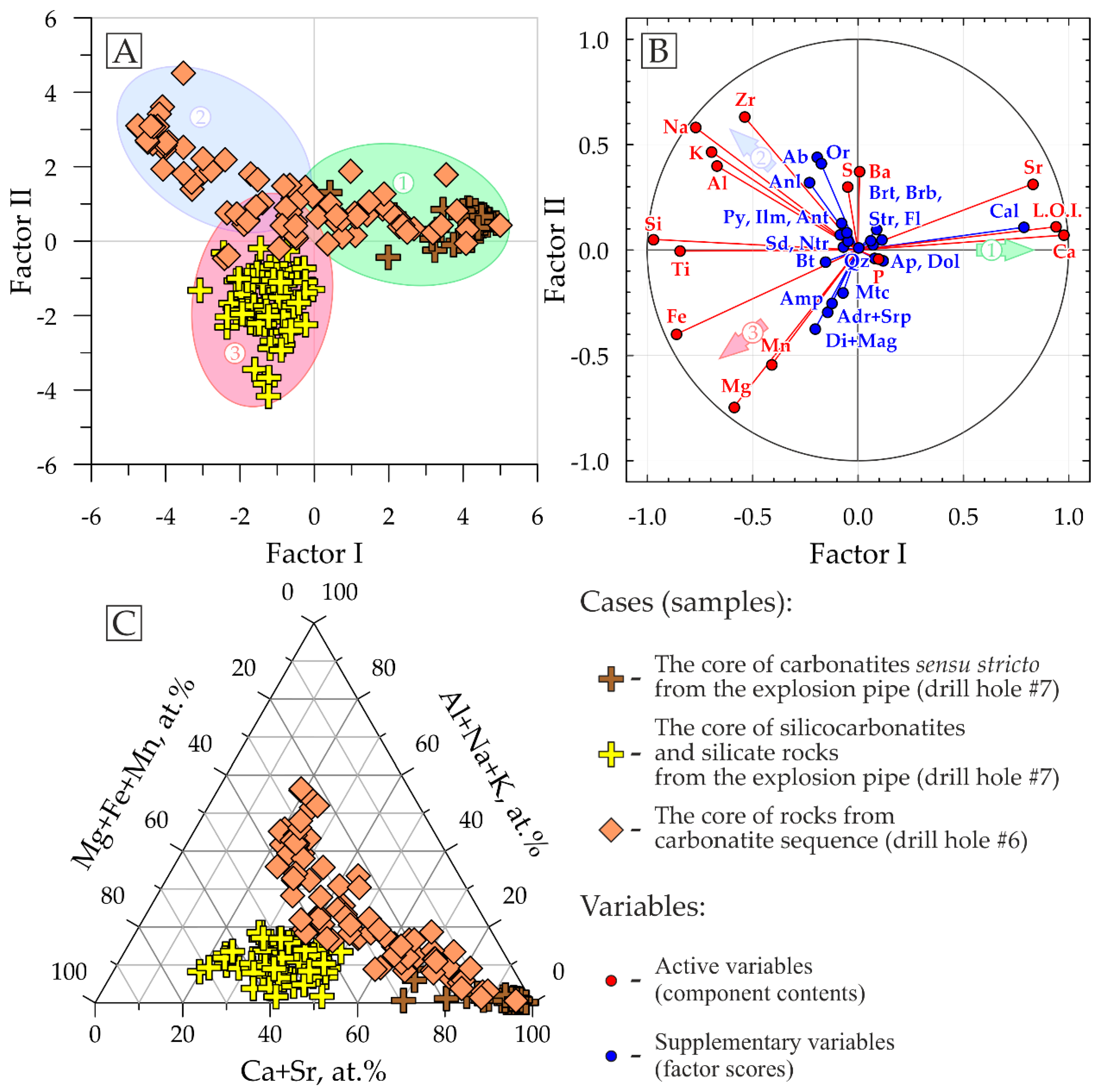
  • The influence of vector 1, related to high content of L.O.I., Ca, and Sr in the rock, led to a shift of the figurative points into group 1;
  • High contents of both Si (+Ti) and Na–K–Al (+Zr), with an essential contribution of Ba–Sr–S, caused a shift of points along vector 2 (towards group 2); and
  • High contents of Si (+Ti) and Mg–Fe (+Mn) resulted in the shifting of points along vector 3 (towards group 3).
The listed components were used as co-ordinates of the barycentric diagram (Figure 7C). The symbolic points of the composition of the samples plotted on it were divided in the same way as on the factor plane in the coordinates Factor I–Factor II (see Figure 7A,C). This circumstance confirms the effectiveness of classical factor analysis in data sorting.
To interpret the above geochemical vectors and groups, we projected the scores of mineralogically explained factors onto the factor plane of Factors I and II (see Figure 7B, blue points). These FSs were supplementary variables (i.e., they did not participate in factor extraction). Their position relative to the active geochemical variables (see Figure 7B, red points) allowed us to draw the following conclusions:
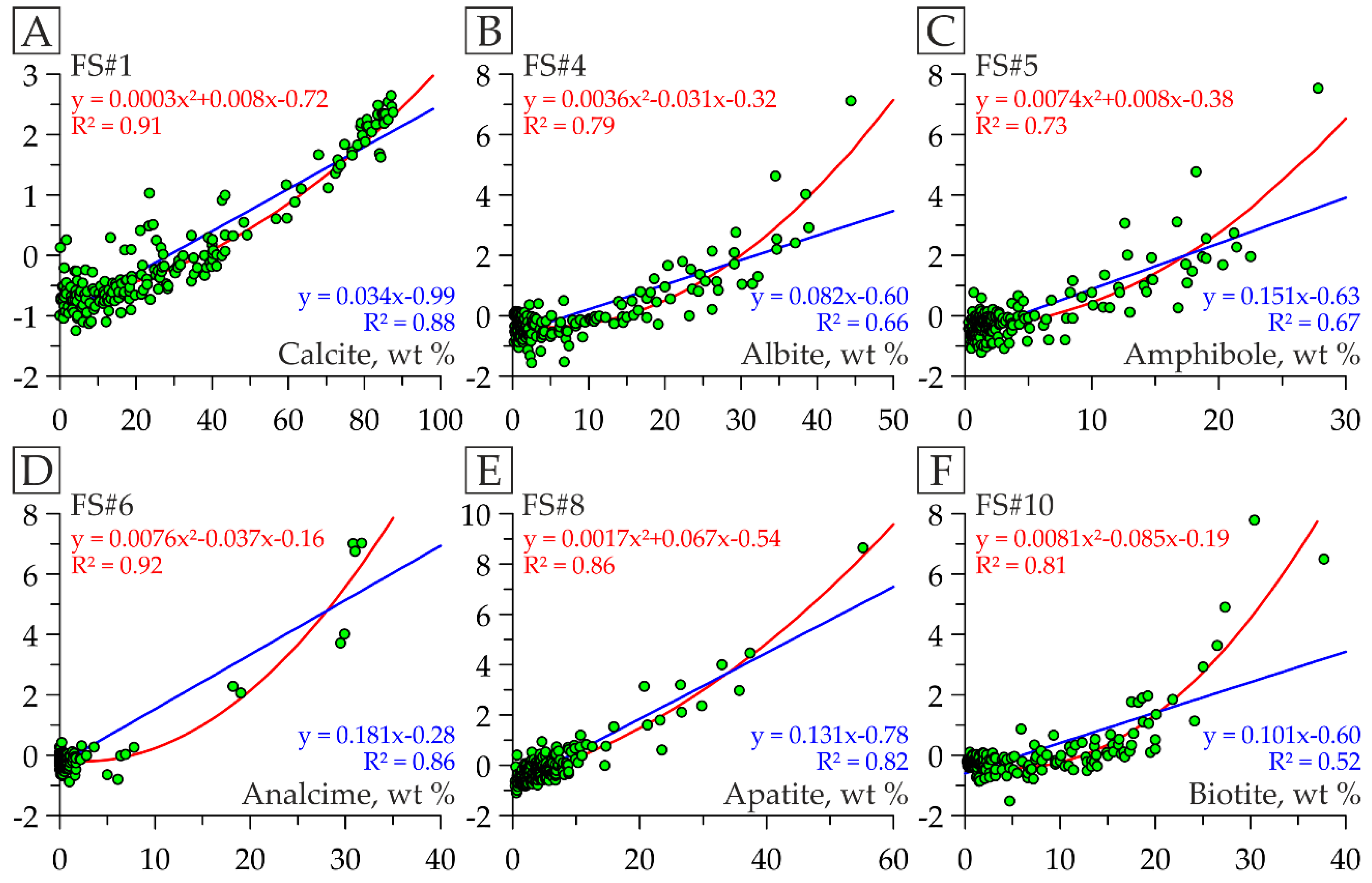
  • Vector 1 (and the corresponding group) was associated with calcite content in the rock. Consequently, group 1 predominantly represented calciocarbonatites (apparently being rich in strontium);
  • Vector 2 was due to the presence of albite, orthoclase, and sometimes analcime (±natrolite) in the rock. Thus, group 2 included samples rich in alkaline salic minerals; and
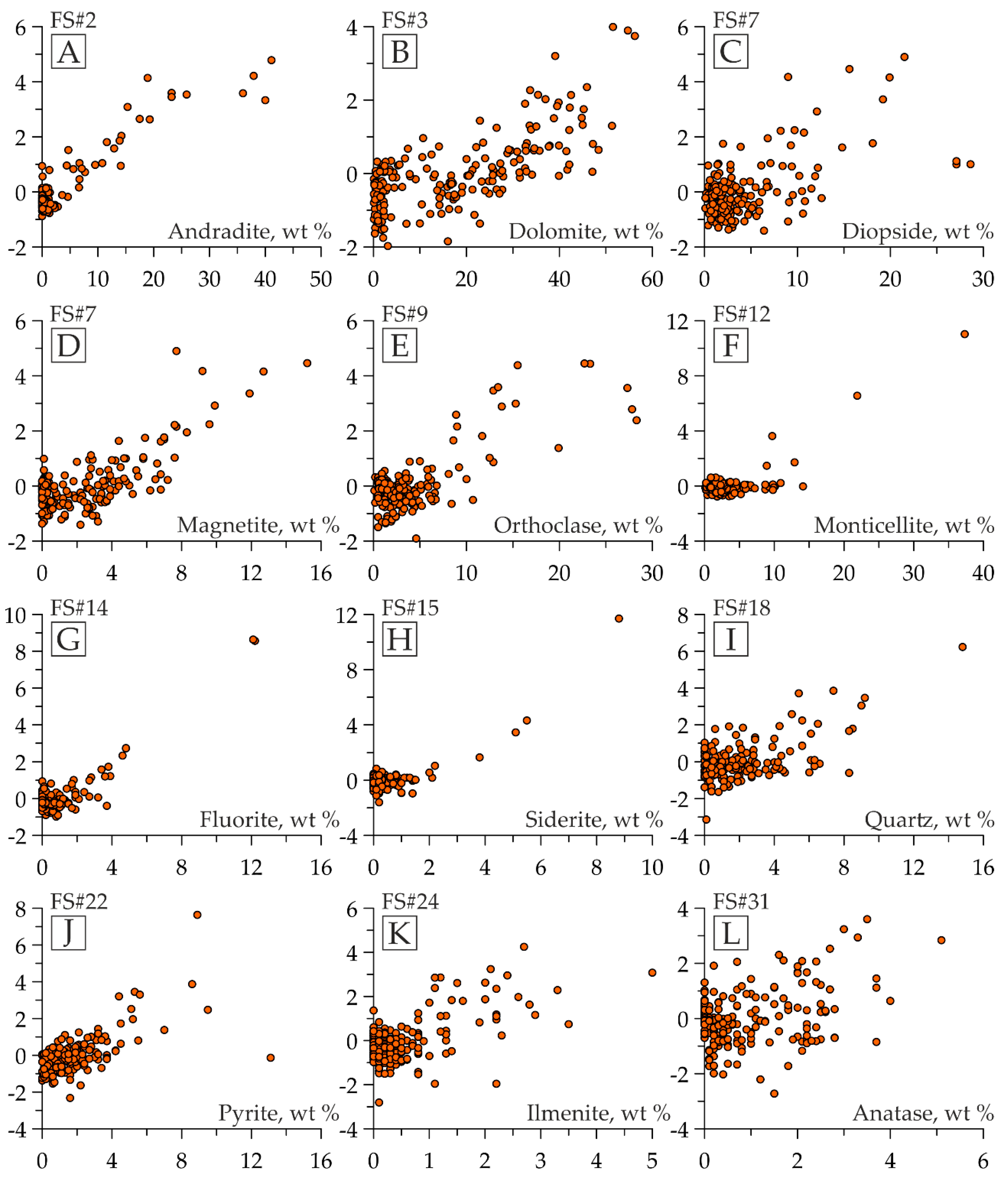
  • Vector 3 responded to the presence of diopside, magnetite, andradite, monticellite, amphibole, serpentine (secondary phase), and/or biotite. Thus, group 3 included rocks rich in femic minerals.
Geochemical analysis showed that the first group included carbonatites sensu stricto (mainly calcium, SiO2 < 20 wt%), both from the explosion pipe (drill core #7) and from the carbonatite sequence (drill core #6). The second group comprised silicocarbonatites and carbonate-rich aluminosilicate rocks from the carbonatite sequence, while the third group included silicocarbonatites and carbonate-rich silicate rocks from the explosion pipe (see Figure 7A). Petrographic–mineralogical investigations fully confirmed these assumptions about the mineral composition, as deduced from the analysis of supplementary variables (factor scores). The positions of active (geochemical) and supplementary (mineralogical) variables on the factor plane in Factor I–Factor II co-ordinates (see Figure 7B) allowed for further statistically sound inferences:
  • Titanium oxides (anatase and ilmenite) gravitated toward group 2, being rich in alkaline sialic minerals. However, titanium did not participate in the discrimination of groups 2 and 3. This suggests that the rocks of both groups were rich in titanium. However, in group 3, phases hosting Ti were not oxides but silicates such as biotite and/or garnet (as confirmed by EPMA);
  • The position of the “dolomite” variable (as well as the “apatite” variable) near the origin in the coordinate system suggests that the presence/absence of this mineral was irrelevant in the division into the groups noted above. This may indicate that all studied rocks of the complex were equally subjected to dolomite mineralization and, therefore, this process was superimposed;
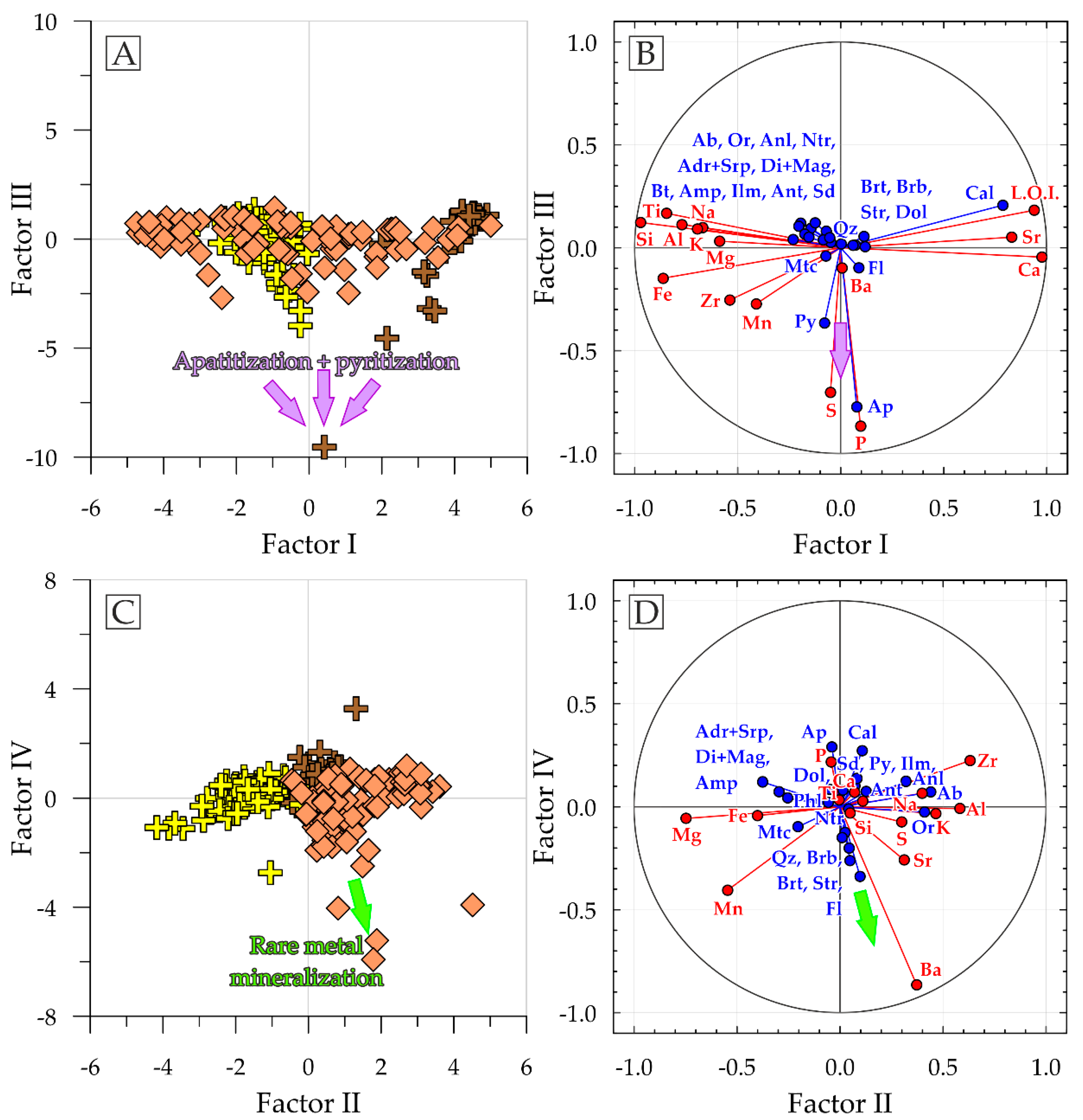
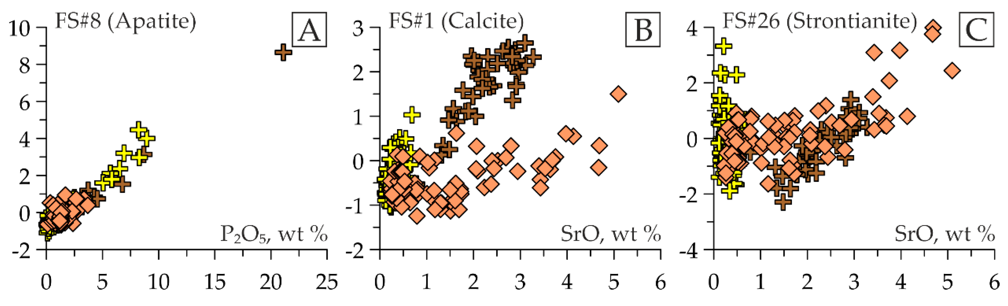
  • None of the considered factors tracked the presence of quartz (supposedly, its content is nearly equal in all types of rocks). Several mineral phases (e.g., apatite, baryte, strontianite, burbankite, and fluorite) exhibited a barely noticeable relationship to the considered separation of samples into groups. Nevertheless, the FSs of these phases were related to other factors identified by classical FA. For example, the scores of apatite and pyrite factors were close to the positive pole of the previously mentioned “phosphate” Factor III (FIIILAp = 0.77 and FIIILPy = 0.37; see Figure 8A,B). The scores of the burbankite, baryte, strontianite, fluorite, and quartz factors formed a shift vector towards the positive pole of the “baryte” Factor IV (Figure 8C,D). In the studied rocks, these minerals constitute a specific mineral paragenesis superimposed onto the earlier associations.
Thus, we determined the main trends in the mineralogical and geochemical evolution of carbonatites and aluminosilicate rocks of the Kontozero Devonian carbonatite paleovolcano.
Additional information can be obtained by direct comparison of the FS values and the content of individual elements (Figure 9); for example, the “FS of apatite factor–P2O5 content” diagram displayed a distinct linear trend (Figure 9A). Consequently, in the studied rock collection, only one mineral (apatite) hosts phosphorus. Among the identified groups, the rocks from the explosion pipe (both carbonatites and silicate carbonate-rich varieties) were most affected by apatite mineralization. In contrast, strontium is hosted by several minerals (e.g., calcite and strontianite), which reflects the presence of several divergent trends in the FS–SrO plots (Figure 9B,C). Silicate carbonate-bearing rocks from the explosion pipe have low strontium content, even at high FSs of strontianite (Figure 9C). This fact implies that strontianite is not the primary strontium concentrator. In the “FSs of strontianite factor–SrO content” diagram (Figure 9C), the carbonatites sensu stricto from the explosion pipe and the entire set of carbonatite sequence rocks jointly form a single trend. Nevertheless, in the “FSs of calcite factor–SrO content” diagram (Figure 9B), the trend of the carbonatite sequence rocks has a steeper slope than that of carbonatites sensu stricto from the explosion pipe. Hence, the highest content of strontium impurity refers to the calcite of rocks from the carbonatite sequence, as confirmed by the EPMA results. Similarly, it is possible to assess the relationship between the content of any identified mineral (expressed through the FS of the corresponding factor) and the concentration of a chemical component of interest in the rock.

4. Conclusions

The major perspectives of factor scores discovered in this study include: (1) rapid qualitative searching for rock samples abundant in (or devoid of) a particular mineral; (2) visualization of the distribution of such rocks in the space of a geological object; (3) when combined with the determination of the mineral composition by routine techniques, the advancement from the qualitative to semiquantitative analysis. Importantly, additional (routine) techniques are required only for a few samples with maximum and minimum FSs, which can be determined from the factor analysis set of phases. These benefits dramatically simplify and speed up the research process.
The use of FSs in classical FA as independent variables characterizing mineral content makes it possible to relate mineralogical and geochemical data numerically. This approach provides a mineralogical–geochemical classification of the studied rocks and reveals the main features of their mineralogical and geochemical evolution. The graphical comparison of FSs and element content elucidates the role of each mineral in the distribution of chemical components in the rock.
Factor analysis of a cumulative XRF and XRPD data set provided all the above information (i.e., qualitative and semiquantitative estimates of the mineral composition; distribution of minerals in the structure of the object; the relationship between the mineral composition and petrochemical characteristics of rocks) in the first stages of research, even in the absence of preliminary mineralogical data on the studied rocks. In turn, this information forms a basis for further, more detailed investigations using standard methods.

Supplementary Materials

The following are available online at https://0-www-mdpi-com.brum.beds.ac.uk/2073-4352/10/10/873/s1, Table S1: Raw diffraction patterns of the samples; Table S2: The measured contents of major elements; Table S3: Factor scores of the samples.

Author Contributions

Conceptualization, E.F.; methodology, E.K.; formal analysis, P.K.; Investigation, E.F., E.K., and P.K.; Writing—Original Draft Preparation, E.F. and E.K.; Visualization, E.K. All authors have read and agreed to the published version of the manuscript.

Funding

This research was funded by the Russian Science Foundation, grant number № 19-77-10039.

Acknowledgments

Core sampling was carried out in TFGI NWFD (Apatity, Russia) under the GI KSC RAS research topic № 0226-2019-0053. The authors express their deepest gratitude to the TFGI NWFD employees for their assistance and to Sidorov M.Yu (GI KSC RAS, Apatity, Russia) for his help with sample preparation. Thanks are due to Chuparina E.V. (IGC SB RAS, Irkutsk, Russia) for XRF analysis. The authors express their sincere gratitude to S.I. Korneev and I.K. Kotova (IES SPbSU) for inculcating interest in factor analysis.

Conflicts of Interest

The authors declare no conflict of interest.

Appendix A

Mineral map numbers from the XRPD database POW_COD [34], the CIF files of which were used for this research are the following: Quartz—1011159; Strontianite—9000227; Monticellite—9001074; Dolomite—9001245; Ferri-eckermannite (amphibole)—9001606; Albite—9001630; Fluorapatite—9001880; Antigorite (serpentine)—9003999; Diopside—9004210; Natrolite—9005047; Orthoclase—9006347; Magnetite—9006920; Fluorite—9007060; Melanite (andradite)—9007075[42]; Analcime—9008207; Anatase—9009086; Clinochlore (chlorite)—9010129; Phlogopite (biotite)—9010864; Ilmenite—9010912; Burbankite—9013840; Pyrite—9015842; Baryte—9016579; Siderite—9016640; Calcite—9016706. Request example: http://www.crystallography.net/cod/1011159.html (Quartz).

References

  1. Wang, X.; Sanei, H.; Dai, S.; Ardakani, O.H.; Isinguzo, N.; Kondla, D.; Tang, Y. A novel method to estimate mineral compositions of mudrocks: A case study for the Canadian unconventional petroleum systems. Mar. Pet. Geol. 2016, 73, 322–332. [Google Scholar] [CrossRef]
  2. Jiang, C.; Chen, Z.; Lavoie, D.; Percival, J.B.; Kabanov, P. Mineral carbon MinC(%) from Rock-Eval analysis as a reliable and cost-effective measurement of carbonate contents in shale source and reservoir rocks. Mar. Pet. Geol. 2017, 83, 184–194. [Google Scholar] [CrossRef]
  3. Nistor, M.M.; Har, N.; Dori, S.M.; Bigi, S.; Gualtieri, A.F. Progress in mineralogical quantitative analysis of rock samples: Application to quartzites from Denali National Park, Alaska Range (USA). Powder Diffr. 2016, 31, 31–39. [Google Scholar] [CrossRef]
  4. Chayes, F. Petrographie Modal Analysis: An Elementary Statistical Appraisal; John Wiley & Sons, Inc.: New York, NY, USA, 1956. [Google Scholar]
  5. Davis, B.L.; Walawender, M.J. Quantitative mineralogical analysis of granitoid rocks: A comparison of X-ray and optical technique. Am. Mineral. 1982, 67, 1135–1143. [Google Scholar]
  6. Warlo, M.; Wanhainen, C.; Bark, G.; Butcher, A.R.; McElroy, I.; Brising, D.; Rollinson, G.K. Automated Quantitative Mineralogy Optimized for Simultaneous Detection of (Precious/Critical) Rare Metals and Base Metals in A Production-Focused Environment. Minerals 2019, 9, 440. [Google Scholar] [CrossRef] [Green Version]
  7. Gu, Y. Automated Scanning Electron Microscope Based Mineral Liberation Analysis An Introduction to JKMRC/FEI Mineral Liberation Analyser. J. Miner. Mater. Charact. Eng. 2003, 2, 33–41. [Google Scholar] [CrossRef]
  8. Hrstka, T.; Gottlieb, P.; Skála, R.; Breiter, K.; Motl, D. Automated mineralogy and petrology—Applications of TESCAN Integrated Mineral Analyzer (TIMA). J. Geosci. 2018, 63, 47–63. [Google Scholar] [CrossRef] [Green Version]
  9. Sindern, S.; Meyer, F.M. Automated Quantitative Rare Earth Elements Mineralogy by Scanning Electron Microscopy. Phys. Sci. Rev. 2016, 1, 1–10. [Google Scholar] [CrossRef]
  10. Gottlieb, P.; Wilkie, G.; Sutherland, D.; Ho-Tun, E.; Suthers, S.; Perera, K.; Jenkins, B.; Spencer, S.; Butcher, A.; Rayner, J. Using quantitative electron microscopy for process mineralogy applications. JOM 2000, 52, 24–25. [Google Scholar] [CrossRef]
  11. Hoal, K.O.; Stammer, J.G.; Appleby, S.K.; Botha, J.; Ross, J.K.; Botha, P.W. Research in quantitative mineralogy: Examples from diverse applications. Miner. Eng. 2009, 22, 402–408. [Google Scholar] [CrossRef]
  12. Madsen, I.C.; Scarlett, N.V.Y.; Webster, N.A.S. Quantitative Phase Analysis. In Uniting Electron Crystallography and Powder Diffraction. NATO Science for Peace and Security Series B: Physics and Biophysics; Kolb, U., Shankland, K., Meshi, L., Avilov, A., David, W.I.F., Eds.; Springer: Dordrecht, The Netherlands, 2012; pp. 207–218. [Google Scholar]
  13. Lutterotti, L. Quantitative Phase Analysis: Method Developments. In Uniting Electron Crystallography and Powder Diffraction. NATO Science for Peace and Security Series B: Physics and Biophysics; Kolb, U., Shankland, K., Meshi, L., Avilov, A., David, W.I.F., Eds.; Springer: Dordrecht, The Netherlands, 2012; pp. 233–242. [Google Scholar]
  14. Pruseth, K.L. Calculation of the CIPW norm: New formulas. J. Earth Syst. Sci. 2009, 118, 101–113. [Google Scholar] [CrossRef] [Green Version]
  15. Mathieu, L.; Trépanier, S.; Daigneault, R. CONSONORM_HG: A new method of norm calculation for mid- to high-grade metamorphic rocks. J. Metamorph. Geol. 2016, 34, 1–15. [Google Scholar] [CrossRef]
  16. Cross, W.; Iddings, J.P.; Pirsson, L.V.; Washington, H.S. A Quantitative Chemico-Mineralogical Classification and Nomenclature of Igneous Rocks. J. Geol. 1902, 10, 555–690. [Google Scholar] [CrossRef]
  17. Fomina, E.; Kozlov, E.; Ivashevskaja, S. Study of diffraction data sets using factor analysis: A new technique for comparing mineralogical and geochemical data and rapid diagnostics of the mineral composition of large collections of rock samples. Powder Diffr. 2019, 34, S59–S70. [Google Scholar] [CrossRef]
  18. Downes, H.; Balaganskaya, E.; Beard, A.; Liferovich, R.; Demaiffe, D. Petrogenetic processes in the ultramafic, alkaline and carbonatitic magmatism in the Kola Alkaline Province: A review. Lithos 2005, 85, 48–75. [Google Scholar] [CrossRef] [Green Version]
  19. Bulakh, A.G.; Ivanikov, V.V.; Orlova, M.P. Overview of carbonatite-phoscorite complexes of the Kola Alkaline Province. In Phoscorites and Carbonatites from Mantle to Mine; Wall, F., Zaitsev, A.N., Eds.; Mineralogical Society of Great Britain and Ireland: London, UK, 2004; pp. 1–43. ISBN 9780903056229. [Google Scholar]
  20. Kramm, U.; Kogarko, L.N.; Kononova, V.A.; Vartiainen, H. The Kola Alkaline Province of the CIS and Finland: Precise Rb-Sr ages define 380–360 Ma age range for all magmatism. Lithos 1993, 30, 33–44. [Google Scholar] [CrossRef]
  21. Kirichenko, L.A. Kontozero Formation of Carboniferous Rocks in the Kola Peninsula; Nedra: Leningrad, Russia, 1970. [Google Scholar]
  22. Borodin, L.S.; Gladkikh, V.S. New petrographic and geochemical data on the volcanogenic alkaline rocks of the Kontozero formation. In New Data on the Geology, Mineralogy, and Geochemistry of Alkaline Rocks; Borodin, L.S., Ed.; Nauka: Moscow, Russia, 1973; pp. 48–55. [Google Scholar]
  23. Pyatenko, I.K.; Saprykina, L.G. Petrological features of alkali basaltic rocks and volcanic carbonatites of the Russian Platform. In Petrology and Petrochemistry of Ore-Bearing Igneous Rock Associations; Bogatikov, O.A., Simon, A.K., Eds.; Nauka: Moscow, Russia, 1981; pp. 233–255. [Google Scholar]
  24. Pyatenko, I.K.; Osokin, E.D. Geochemical features of the Kontozero carbonatite paleovolcano in the Kola Peninsula. Geokhimiya 1988, 25, 723–737. [Google Scholar]
  25. Arzamastsev, A.A.; Petrovsky, M.N. Alkaline volcanism in the Kola Peninsula, Russia: Paleozoic Khibiny, Lovozero and Kontozero calderas. Proc. MSTU 2012, 15, 277–299. [Google Scholar]
  26. Petrovsky, M.N.; Savchenko, E.A.; Kalachev, V.Y. Formation of eudialyte-bearing phonolite from Kontozero carbonatite paleovolcano, Kola Peninsula. Geol. Ore Depos. 2012, 54, 540–556. [Google Scholar] [CrossRef]
  27. Website of IM UB RAS (Miass, Russia). Available online: http://www.mineralogy.ru (accessed on 3 July 2020).
  28. Amosova, A.A.; Panteeva, S.V.; Chubarov, V.M.; Finkelshtein, A.L. Determination of major elements by wavelength-dispersive X-ray fluorescence spectrometry and trace elements by inductively coupled plasma mass spectrometry in igneous rocks from the same fused sample (110 mg). Spectrochim. Acta Part B At. Spectrosc. 2016, 122, 62–68. [Google Scholar] [CrossRef]
  29. Website of IG SB RAS (Irkutsk, Russia). Available online: http://www.igc.irk.ru (accessed on 3 July 2020).
  30. Qualx2 Software. Available online: http://www.ba.ic.cnr.it/softwareic/qualx/ (accessed on 3 July 2020).
  31. Altomare, A.; Corriero, N.; Cuocci, C.; Falcicchio, A.; Moliterni, A.; Rizzi, R. QUALX2.0 : A qualitative phase analysis software using the freely available database POW_COD. J. Appl. Crystallogr. 2015, 48, 598–603. [Google Scholar] [CrossRef]
  32. MAUD Software. Available online: http://maud.radiographema.eu/ (accessed on 3 July 2020).
  33. Lutterotti, L.; Matthies, S.; Wenk, H.-R. MAUD: A friendly Java program for materials analysis using diffraction. Int. Union Crystallogr. Comm. Powder Diffr. Newsl. 1999, 21, 14–15. [Google Scholar]
  34. Gražulis, S.; Daškevič, A.; Merkys, A.; Chateigner, D.; Lutterotti, L.; Quirós, M.; Serebryanaya, N.R.; Moeck, P.; Downs, R.T.; Le Bail, A. Crystallography Open Database (COD): An open-access collection of crystal structures and platform for world-wide collaboration. Nucleic Acids Res. 2012, 40, D420–D427. [Google Scholar] [CrossRef] [PubMed]
  35. Fomina, E.; Kozlov, E.; Bazai, A. Factor Analysis of XRF- and XRPD-data on the Case Study of the Rocks of the Kontozero Carbonatite Complex (NW Russia). Part I: Algorithm. Crystals 2020. [Google Scholar]
  36. Davis, B.L.; Kath, R.; Spilde, M. The Reference Intensity Ratio: Its Measurement and Significance. Powder Diffr. 1990, 5, 76–78. [Google Scholar] [CrossRef]
  37. Rietveld, H.M. A profile refinement method for nuclear and magnetic structures. J. Appl. Crystallogr. 1969, 2, 65–71. [Google Scholar] [CrossRef]
  38. Stephens, P.W. Rietveld Refinement. In Uniting Electron Crystallography and Powder Diffraction. NATO Science for Peace and Security Series B: Physics and Biophysics; Kolb, U., Shankland, K., Meshi, L., Avilov, A., David, W.I.F., Eds.; Springer: Dordrecht, The Netherlands, 2012; pp. 15–26. [Google Scholar]
  39. Kozlov, E.; Fomina, E. Geological interpretation of the results of factor analysis of XRF- and XRD-data on carbonatite and aluminosilicate rocks of the Kontozero alkaline complex (Kola Peninsula, NW Russia). In IOP Conference Series: Earth and Environmental Science; IOP Publishing: Bristol, UK, 2020; in press. [Google Scholar]
  40. Bish, D.L.; Post, J.E. Quantitative mineralogical analysis using the Rietveld full-pattern fitting method. Am. Mineral. 1993, 78, 932–940. [Google Scholar]
  41. Jöreskog, K.G.; Klovan, J.E.; Reyment, R.A. Geological Factor Analysis; Elsevier: Amsterdam, The Netherlands, 1976. [Google Scholar]
  42. Quartieri, S.; Boscherini, F.; Chaboy, J.; Dalconi, M.C.; Oberti, R.; Zanetti, A. Characterization of trace Nd and Ce site preference and coordination in natural melanites: A combined X-ray diffraction and high-energy XAFS study. Phys. Chem. Miner. 2002, 29, 495–502. [Google Scholar] [CrossRef]
Figure 1. Geological scheme of Kontozero paleocaldera [23]. 1—Zeolite–ankerite–dolomite (± albite) metasomatic rocks; 2—Carbonatite–picrite explosion pipe; (3–6) Kontozero formation: 3—Carbonatite agglomerate tuffs and tuffaceous breccias of vent facies; 4—Carbonatite sequence; 5—Melilitite sequence; 6—Augitite sequence; 7—Terrigenous–volcanic sequence of the Lovozero formation; 8—Alkaline and nepheline syenites; 9—Pyroxenites; 10—Archean gneiss and granite–gneiss; (11–13) Geological boundaries: 11—Between sequences; 12—Between facial varieties; 13—Intrusive; 14—Faults; 15—Drill holes (the rectangles mark the examined intervals). The subfigure shows the location of Kontozero in the Kola region.
Crystals 10 00873 g001
Figure 2. Examples of the functional relationships between factor scores (FS) and semiquantitative estimates of the mineral contents. Factor numbers are shown after the “#” symbol.
Crystals 10 00873 g002
Figure 3. Approximation models of the functional relationships between the FSs and the semiquantitative estimates of mineral contents. Linear trends are blue lines; polynomial trends are red lines.
Crystals 10 00873 g003
Figure 4. Comparison of graphs of calcite content (blue lines) and calcite FS (red lines) in cores of drill holes: (A) #7 (explosion pipe) and (B) #6 (carbonatite sequence); (C) ranked range of FS values of the calcite factor.
Crystals 10 00873 g004
Figure 5. (A,B) The ranked range of the amphibole FSs. In (A), the point diameters are proportional to the semiquantitative estimates of amphibole abundance. In (B), the coloration of the figurative points reflects the division of the collection into four groups, according to the amphibole content in the samples: red, maximum content; orange, high content; green, low content; blue, no amphibole (detailed explanations are in the text). The inset shows the amphibole peak, which served as determinant for referring to the groups. (C) The distribution of the amphibole FSs in sections of the studied cores.
Crystals 10 00873 g005
Figure 6. The ranked range of FSs for (A) andradite, (B) analcime, and (C) monticellite (the contents of the corresponding minerals in some samples are indicated); the FS distribution for (D) andradite, (E) analcime, and (F) monticellite in the drill cores. Figure from [39].
Crystals 10 00873 g006
Figure 7. (A) Projection of the cases onto the factor-plane (Factor I vs. Factor II), the fields outline the sample groups (details are given in the text); (B) projection of the variables onto the factor-plane (Factor I vs. Factor II); (C) figurative points of rock compositions on the barycentric diagram in coordinates [Ca + Sr]–[Mg + Fe + Mn]–[Al + Na + K] (atomic%), selected based on the results of classical FA.
Crystals 10 00873 g007
Figure 8. Projection of the (A) cases and (B) variables onto the factor-plane in the “Factor I–Factor III” coordinates. Projection of the (C) cases and (D) variables onto the factor-plane in the “Factor II–Factor IV” coordinates. The legend is the same as in Figure 7.
Crystals 10 00873 g008
Figure 9. Figurative points of the samples on the diagrams in the coordinates (A) FSs of apatite factor–P2O5 content (wt%); (B) FSs of calcite factor–SrO content (wt%); (C) FSs of strontianite factor–SrO content (wt%). Legend: peach rhombs—undifferentiated rocks of carbonatite sequence (drill core #6); brown crosses—carbonatites sensu stricto (mostly calcium) from explosion pipe (drill core #7); yellow crosses—silicocarbonatites and carbonate-bearing silicate rocks from the explosion pipe (drill core #7).
Crystals 10 00873 g009

