Computational Approach to Dynamic Systems through Similarity Measure and Homotopy Analysis Method for Renewable Energy


1
KMUTTFixed Point Research Laboratory, Room SCL 802 Fixed Point Laboratory, Science Laboratory Building, Department of Mathematics, Faculty of Science, King Mongkut’s University of Technology Thonburi (KMUTT), Bangkok 10140, Thailand
2
Center of Excellence in Theoretical and Computational Science (TaCS-CoE), Science Laboratory Building, Faculty of Science, King Mongkut’s University of Technology Thonburi (KMUTT), 126 Pracha-Uthit Road, Bang Mod, Thrung Khru, Bangkok 10140, Thailand
3
Department of Mathematics, Division of Science and Technology, University of Education, Lahore 54000, Pakistan
4
Department of Medical Research, China Medical University Hospital, China Medical University, Taichung 40402, Taiwan
5
Renewable Energy Research Centre, Department of Teacher Training in Electrical Engineering, Faculty of Technical Education, King Mongkut’s University of Technology North Bangkok, 1518 Pracharat 1 Road, Wongsawang, Bangsue, Bangkok 10800, Thailand
*
Authors to whom correspondence should be addressed.
Crystals 2020, 10(12), 1086; https://0-doi-org.brum.beds.ac.uk/10.3390/cryst10121086
Submission received: 6 October 2020
/
Revised: 9 November 2020
/
Accepted: 10 November 2020
/
Published: 27 November 2020
(This article belongs to the Special Issue Structural, Magnetic, Dielectric, Electrical, Optical and Thermal Properties of Nanocrystalline Materials: Synthesis, Characterization and Application)
Abstract
:To achieve considerably high thermal conductivity, hybrid nanofluids are some of the best alternatives that can be considered as renewable energy resources and as replacements for the traditional ways of heat transfer through fluids. The subject of the present work is to probe the heat and mass transfer flow of an ethylene glycol based hybrid nanofluid (Au-ZnO/CHO) in three dimensions with homogeneous-heterogeneous chemical reactions and the nanoparticle shape factor. The applications of appropriate similarity transformations are done to make the corresponding non-dimensional equations, which are used in the analytic computation through the homotopy analysis method (HAM). Graphical representations are shown for the behaviors of the parameters and profiles. The hybrid nanofluid (Au-ZnO/CHO) has a great influence on the flow, temperature, and cubic autocatalysis chemical reactions. The axial velocity and the heat transfer increase and the concentration of the cubic autocatalytic chemical reactions decreases with increasing stretching parameters. The tangential velocity and the concentration of cubic autocatalytic chemical reactions decrease and the heat transfer increases with increasing Reynolds number. A close agreement of the present work with the published study is achieved.
1. Introduction
Energy has a crucial role in the prosperity and development of any country. The daily consumed energy resources like natural gas, oil, and coal are certain to vanish with the passage of time because these are huge sources of energy and are being depleted due to their limited availability. To cope with such a situation, the replenishment of the world’s energy is of utmost concern, making it is a basic requirement to search for some reliable and affordable energy alternatives. Such problems apply to renewable energy systems. Nanoparticles have been shown to solve such constraints because of their remarkable heat transfer capabilities. The application of nanoparticles in the industrial, biomedical, and energy sectors is due to their thermophysical properties. Nanoparticles have seen applications in energy conversion (e.g., fuel cells, solar cells, and thermoelectric devices), energy storage (e.g., rechargeable batteries and super capacitors), and energy saving (e.g., insulation such as aerogels and smart glazes, efficient lightning like light emitting diodes and organic light-emitting diodes). To combat climate change, clean and sustainable energy sources need to be rapidly developed. Solar energy technology converts solar energy directly into electricity, for which high performance cooling, heating, and electricity generation are among the inevitable requirements. In solar collectors, the absorbed incident solar radiation is converted to heat. The working fluid conveys the generated heat for different uses [1]. Ettefaghi et al. [2] worked on a bio-nanoemulsion fuel based on biodegradable nanoparticles to improve diesel engines’ performance and reduce exhaust emissions. Gunjo et al. [3] investigated the melting enhancement of a latent heat storage with dispersed Cu, CuO, and Al2O3 nanoparticles for a solar thermal application. Khanafer and Vafai [4] presented a review on the applications of nanofluids in the solar energy field.
Nanofluids reduce the process time, enhance the heating rates, and improve the lifespan of machinery [5]. Nanofluids have seen applications in power saving, manufacturing, transportation, healthcare, microfluidics, nano-technology, microelectronics, etc. Recently, nano-technology has attracted great attraction from scientists [6]. Nanoparticles are the most interesting technology to introduce novel, environmentally friendly chemical and mechanical polishing slurries to fabricate effective materials [7]. Thermal conductivity is of great importance and is enhanced by the incorporation of nanoparticles in the base fluid [8]. Hamilton and Crosser [9] studied the thermal conductivity of a heterogeneous two component system. Nanofluids were obtained by the addition of nanoparticles to the base fluids, and they have gained popularity since the work of Choi and Eastman [10]. Vallejo et al. [11] analyzed the internal aspects of the fluid for six carbon-based nanomaterials in a rotating rheometer with a double conic shape containing a typical sheet. Alihosseini and Jafari [12] investigated a three-dimensional computational fluid dynamics model for an aluminum foam and nanoparticles with heat transfer using a number of cylinders having different configurations through a permeable medium. Sheikholeslami et al. [13], working with a ethylene glycol nanofluid, discussed the electric field, thermal radiation, and nanoparticle shape factors of a ferrofluid by showing that the platelet shape led to enhanced convective flow. Al-Kouz et al. [14] applied computational fluid dynamics to analyze entropy generation in a rarefied time dependent, laminar two-dimensional flow of an air-aluminum oxide nanofluid in a cavity with a square shape having more than one solid fin at the heated wall where the optimization procedure was adopted to show the conditions by which the overall entropy generation was reduced. Atta et al. [15] modified the asphaltenes isolated from crude oil to work as capping agents for the synthesis of hydrophobic silica to investigate the surface charge of hydrophobic silica nanoparticles, the chemical structure, the particle size, and the surface morphology. Rout et al. [16] presented the three and higher order nonlinear thin film study and optics fabricated with gold nanoparticles. They obtained the solution via spin-coating techniques to achieve the highest values of nonlinear absorption coefficient, nonlinear refractive index and saturation intensity. Alvarez-Regueiro et al. [17] experimentally determined the heat transfer coefficients and pressure drops of four functionalized graphene nanoplatelet nanofluids for heat transfer enhancement to discuss the nanoadditive loading, temperature and Reynolds number. Alsagri et al. [18] elaborated the heat and mass transfer flow of single walled and multi walled carbon nanotubes past a stretchable cylinder by investigating that the heat transfer enhances with the high values of nanoparticles concentration of single walled carbon nanotubes compared to that of multi walled carbon nanotubes. Working on transverse vibration, Mishra et al. [19] comparatively investigated a computational fluid dynamic model for water based nanofluid through a pipe subject to superimposed vibration, applied to the wall to increase the heat transfer in axial direction while vibration effect is decreased for pure liquid and is increased for nanofluid. Abbas et al. [20] achieved the results that in the heat and mass transfer flow of Cross nanofluid, the Bejan number was intensified for the high values of thermal radiation parameter. Some discussion on nanofluids and other relevant studies can be found in the references [21,22,23,24,25,26,27,28,29,30,31,32,33,34,35,36,37,38,39,40,41,42,43,44,45,46,47,48,49,50,51,52,53,54,55].
Mono-nanofluids represent enhanced thermal conductivity and good rheological characteristics, but still they have some weak characteristics necessary for a particular purpose. By the hybridization process, different nanoparticles are added in a base fluid to make the hybrid nanofluid which has enhanced thermophysical properties and thermal conductivity as well as rheological properties. Ahmad et al. [56] investigated the hybrid nanofluid with activation energy and binary chemical reaction through a moving wedge taken into account the Darcy law of porous medium, heat generation, thermal slip, radiation, and variable viscosity. Dinarvand and Rostami [57] presented the ZnO-Au hybrid nanofluid when 15 gm of nanoparticles are added into the 100 gm base fluid, the heat transfer enhances more than 40% compared to that of the regular fluid.
Homogeneous-heterogeneous chemical reactions have important applications in chemical industries. Ahmad and Xu [58] worked on homogeneous-heterogeneous chemical reactions in which the reactive species were of regular size reacting with other species in a nanofluid to show more realistic mathematical model physically. Hayat et al. [59] elaborated the Xue nanofluid model to study the carbon nanotubes nanofluids in rotating systems incorporating Darcy–Forchheimer law, homogeneous-heterogeneous chemical reactions and optimal series solutions. Suleman et al. [60] addressed the homogeneous-heterogeneous chemical reactions in Ag-HO nanofluid flow past a stretching sheet with Newtonian heating to prove that concentration field was decreased for the increasing strength of homogeneous-heterogeneous chemical reactions.
In the literature, interesting studies exists like [5] which investigates the electrical conductivity, structural and optical properties of ZnO. In study [6], the theoretical and experimental results of electric current and thermal conductivity of HO-ethylene glycol based TiO have been obtained. The study [7] relates to the oxide-ethylene glycol nanofluid with different sizes of nanoparticles. Due to the applications of the above studies, it is desire to investigate the ethylene glycol based Au-ZnO hybrid nanofluid flow with heat transfer and homogeneous-heterogeneous chemical reactions in rotating system. The present study has the applications in renewable energy technology, thermal power generating system, spin coating, turbo machinery etc. The solution of the problem is obtained through an effective technique known as homotopy analysis method [61]. Investigations are shown through graphs and discussed in detail.
2. Methods
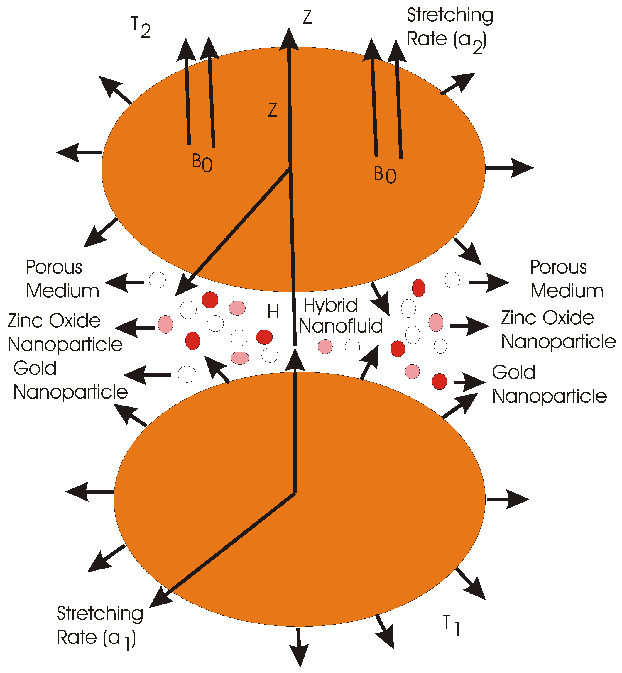
A rotating flow of hydromagnetic, time independent and incompressible hybrid nanofluid between two parallel disks in three dimensions is analyzed. Homogeneous-heterogeneous chemical reactions are also considered. The lower disk is supposed to locate at z = 0 while the upper disk is at a constant distance H apart. The velocities and stretching on these disks are (, ) and (a, a), respectively while the temperatures on these disks are T and T, respectively. A magnetic field of strength B is applied in the direction of z-axis (please see Figure 1). Ethylene glycol is chosen for the base fluid in which zinc oxide and gold nanoparticles are added.
For cubic auto-catalysis, the homogeneous reaction is
The first order isothermal reaction on the surface of catalyst is
where B and C denote the chemical species with concentrations b and c, respectively. k and k are the rate constants.
Cylindrical coordinates (r, , z), are applied to provide the thermodynamics of hybrid nanofluid as [57,58,59]
The boundary conditions are
where u(r, ϑ, z), v(r, ϑ, z) and w(r, ϑ, z) are the components of velocity, P is the pressure. S is the permeability of porous medium, S = is the non-uniform inertia coefficient of porous medium with C as the drag coefficient. Temperature of hybrid nanofluid is T and B = (0, 0, B) is the magnetic field. is the Stefan Boltzmann constant and k is the absorption coefficient. For the hybrid nanofluid, the important quantities are (density), (dynamic viscosity), (electrical conductivity), (c) (heat capacity) and k (thermal conductivity). The subscript “hnf” shows the hybrid nanofluid. For the thermal conductivity, the mathematical formulation is obtained via Hamilton–Crosser model [9] as
where n is the empirical shape factor for the nanoparticle whose value is given in Table 1.
The subscript “f” denotes the base fluid namely ethylene glycol and the subscript “nf” is used for nanofluid. and (c) are the density and heat capacity at specified pressure of nanoparticles, respectively. is the first nanoparticle volume fraction while is the second nanoparticle volume fraction which can be formulated as [57].
where m, m and m are, respectively the mass of first nanoparticle, mass of the second nanoparticle and mass of the base fluid. is the total volume fraction of zinc oxide and gold nanoparticles.
The thermophysical properties of CHO as well as nanoparticles are given in Table 2.
The mathematical formulations for (density), (dynamic viscosity), (electrical conductivity), (c) (heat capacity) are given in Table 3 where shows the particle concentration.
Following transformations are used
where = is the kinematic viscosity and is the pressure parameter.
Using the values from Equation (18) in Equations (4)–(11), the following eight Equations (19)–(26) are obtained
where () represents the derivative with respect to . B = ×, B = 1 + , B = , B = . k = is the porosity parameter, k = is the inertial parameter due to Darcy Forchheimer effect. The other non-dimensional parameters are = , Re = , M = , Rd = , Pr = , Ec = , Sc = , k = , k = , k = , k = and k = which are known as rotation parameter, Reynolds number, magnetic field parameter, thermal radiation parameter, Prandtl number, Eckert number, Schmidt number, homogeneous chemical reaction parameter, diffusion coefficient ratio, stretching parameter for lower disks, heterogeneous chemical reaction parameter and stretching parameter at upper disk, respectively.
Regarding the homogeneous-heterogeneous chemical reaction, the quantities B and C may be considered in a special case, i.e., if D is equal to D, then in such a case k equals unity, which leads to
Using Equation (27), Equations (23) and (24) generate
whose corresponding boundary conditions become
By taking derivative of Equation (19) with respect to , it becomes
Considering Equation (21), Equations (25) and (26), the quantity is computed as
Skin Frictions and Nusselt Numbers
The important physical quantities are defined as
where
denotes the sum of shear stress of tangential forces and along radial and tangential directions which are defined as
Using the information of Equations (34) and (35), Equation (33) proceeds to
where = is the Reynolds number.
Another important physical quantity is
where q is the surface temperature defined as
3. Computational Methodology
Following the HAM, choosing the initial guesses and linear operators for the velocities, temperature and homogeneous-heterogeneous chemical concentration profiles as
characterizing
where E(i = 1–10) are the arbitrary constants.
3.1. Zeroth Order Deformation Problems
Introducing the nonlinear operator ℵ as
where j is the homotopy parameter such that j ∈ [0, 1].
Moreover
where , , and are the convergence control parameters.
Boundary conditions of Equation (48) are
Boundary conditions of Equation (49) are
Boundary conditions of Equation (50) are
Boundary conditions of Equation (51) are
Characterizing j = 0 and j = 1, the calculations obtained as
f(ζ,j) becomes f(ζ) and f(ζ) as j assumes the values zero and one. g(ζ,j) becomes g(ζ) and g(ζ) as j assumes the values zero and one. θ(ζ,j) becomes θ(ζ) and θ(ζ) as j assumes the values zero and one. Finally, φ(ζ,j) becomes φ(ζ) and φ(ζ) as j assumes the values zero and one.
Applying Taylor series expansion on the Equations (56)–(59), the results are obtained as
, , and are adjusted to obtain the convergence for the series in Equations (60)–(63) at j = 1, so Equations (60)–(63) transform to
3.2. mth Order Deformation Problems
Considering Equations (48) and (52) for homotopy at mth order as
Considering Equations (49) and (53) for homotopy at mth order as
Considering Equations (50) and (54) for homotopy at mth order as
Considering Equations (51) and (55) for homotopy at mth order as
Adding the particular solutions f(ζ), g(ζ), θ(ζ) and φ(ζ), Equations (68), (71), (74) and (77) yield the general solutions as
4. Results and Discussion
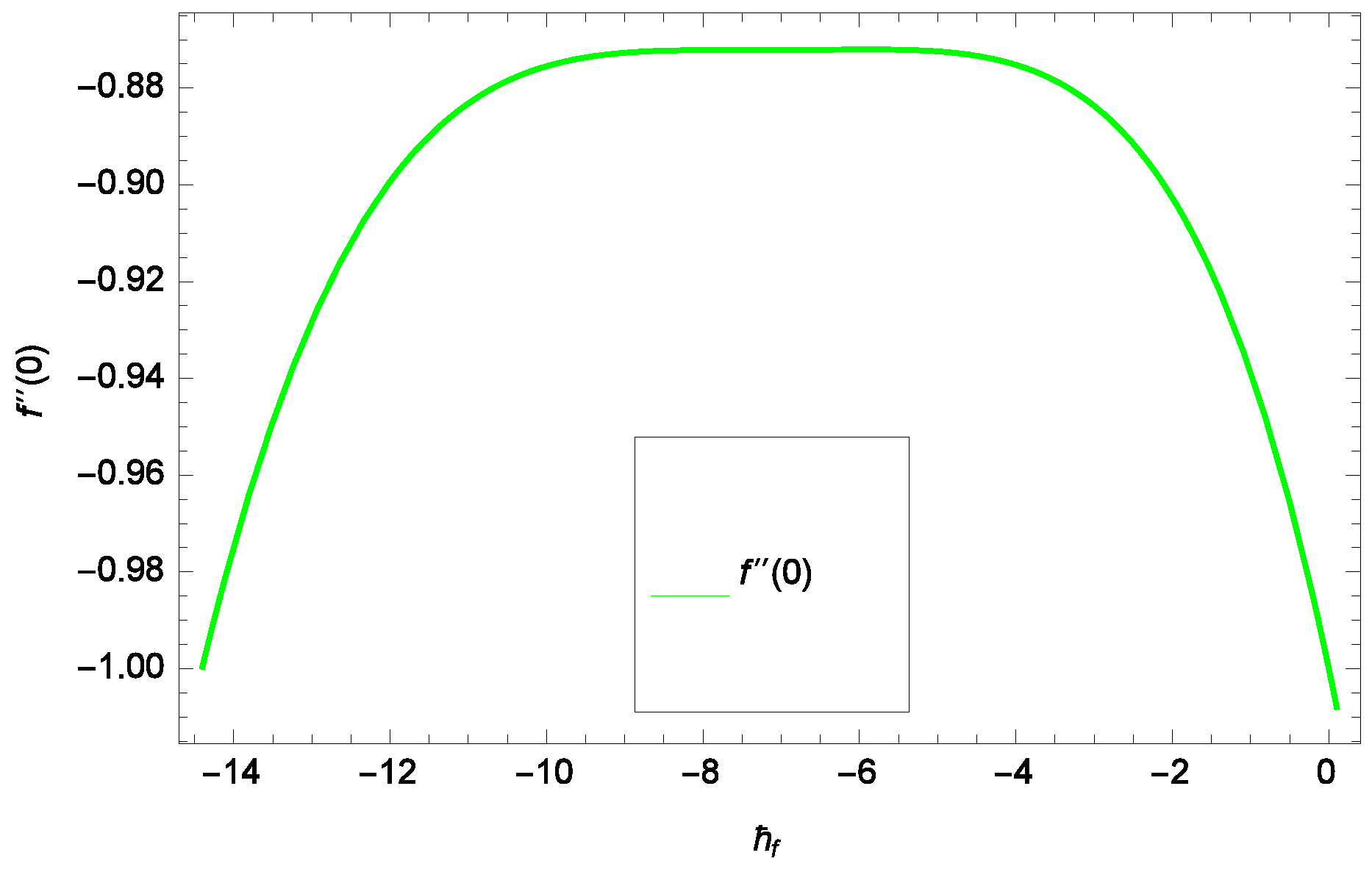
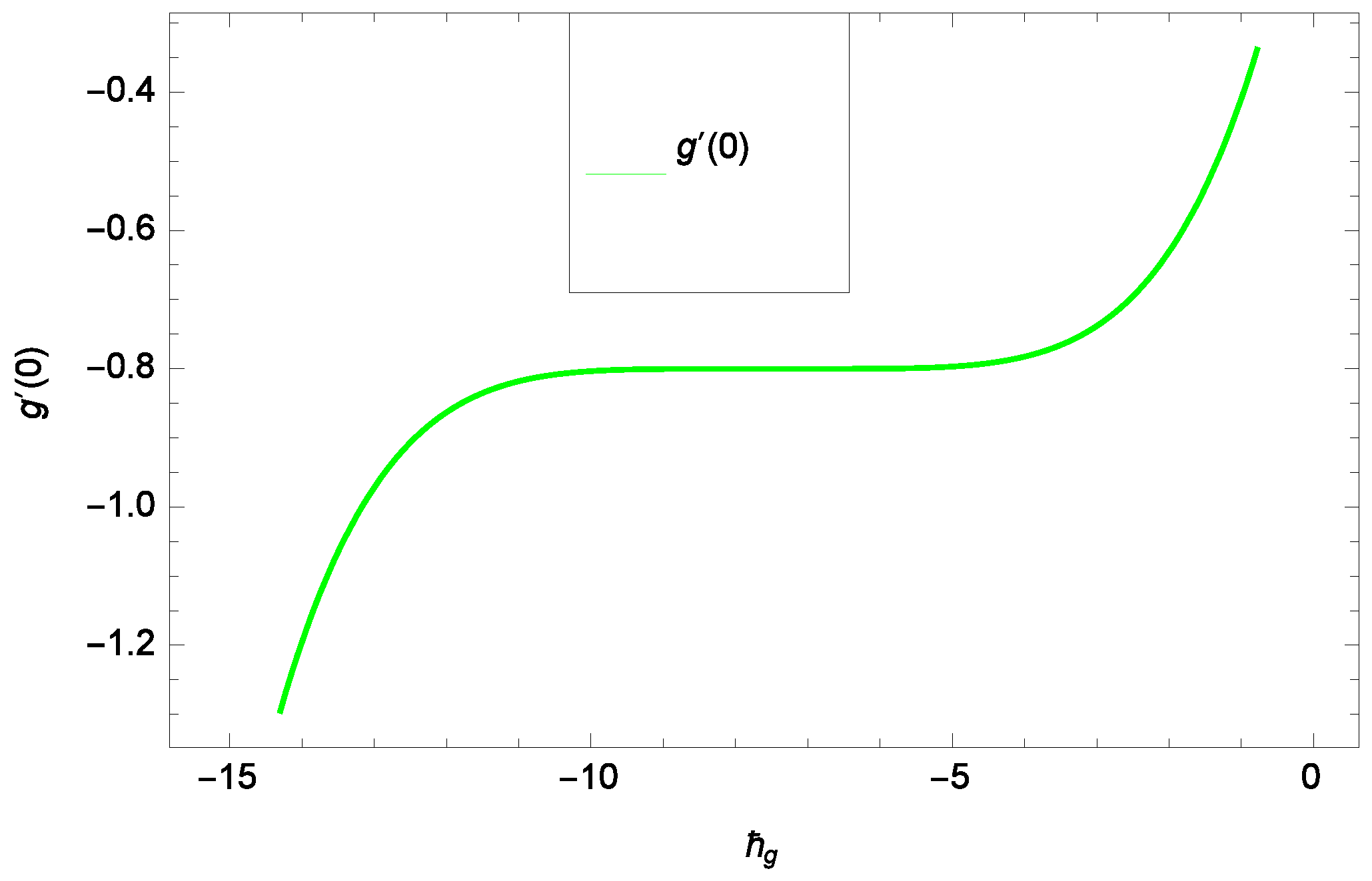
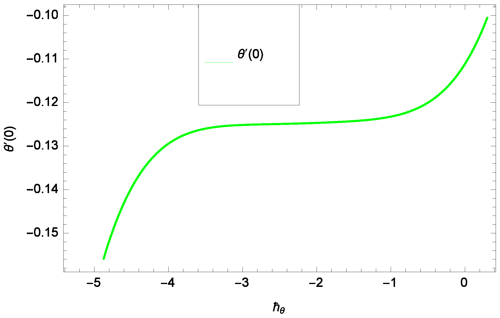
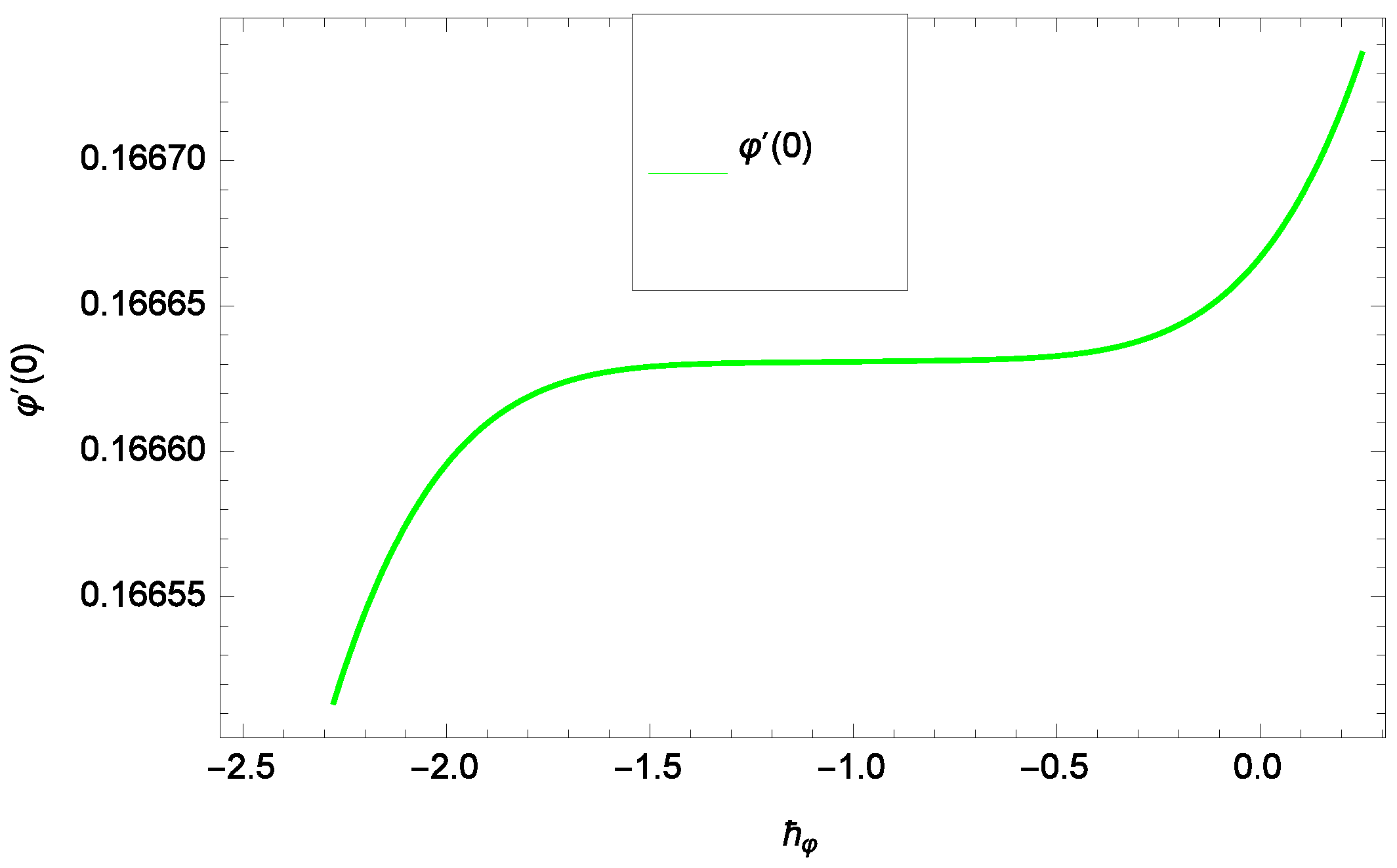
Results and discussion provide the analysis of the problem through the impacts of all the relevant parameters. The non-dimensional Equations (20), (22), (28) and (30) with boundary conditions in Equations (25), (26) and (29) are analytically computed. The performances of different parameters on the velocity profiles with heat and concentration of homogeneous-heterogeneous chemical reactions are shown in the relevant graphs. The streamlines show the internal behaviors of flow. The physical representation of the problem is shown in Figure 1. Liao [61] introduced ℏ-curves for the convergence of the series solution to get the precise and convergent solutions of the problems. ℏ-curves are also called the convergence controlling parameters for solution in the homotopy analysis method (used for solution in the present case). These ℏ-curves specify the range of numerical values. These numerical values (optimum values) are selected from the valid region in straight line. These optimum values of ℏ-curves are selected from the straight lines parallel to the horizontal axis (please see carefully Figure 2, Figure 3, Figure 4 and Figure 5) to control the convergence of problem solution. In the present case, the valid region of each profile ℏ-curve is specified. Therefore, the admissible ℏ-curves for f(ζ), g(ζ), θ(ζ) and φ(ζ) are drawn in the ranges −10.00 ≤ ≤ −4.00, −10.00 ≤ ≤ −5.00, −3.5 ≤ ≤ −2.50 and −1.50 ≤ ≤ −0.50 in Figure 2, Figure 3, Figure 4 and Figure 5, respectively.
4.1. Axial Velocity Profile
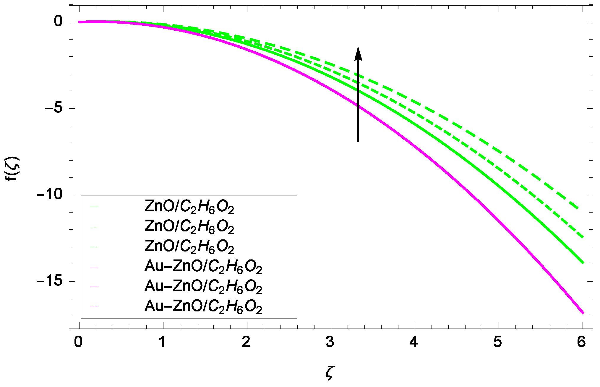
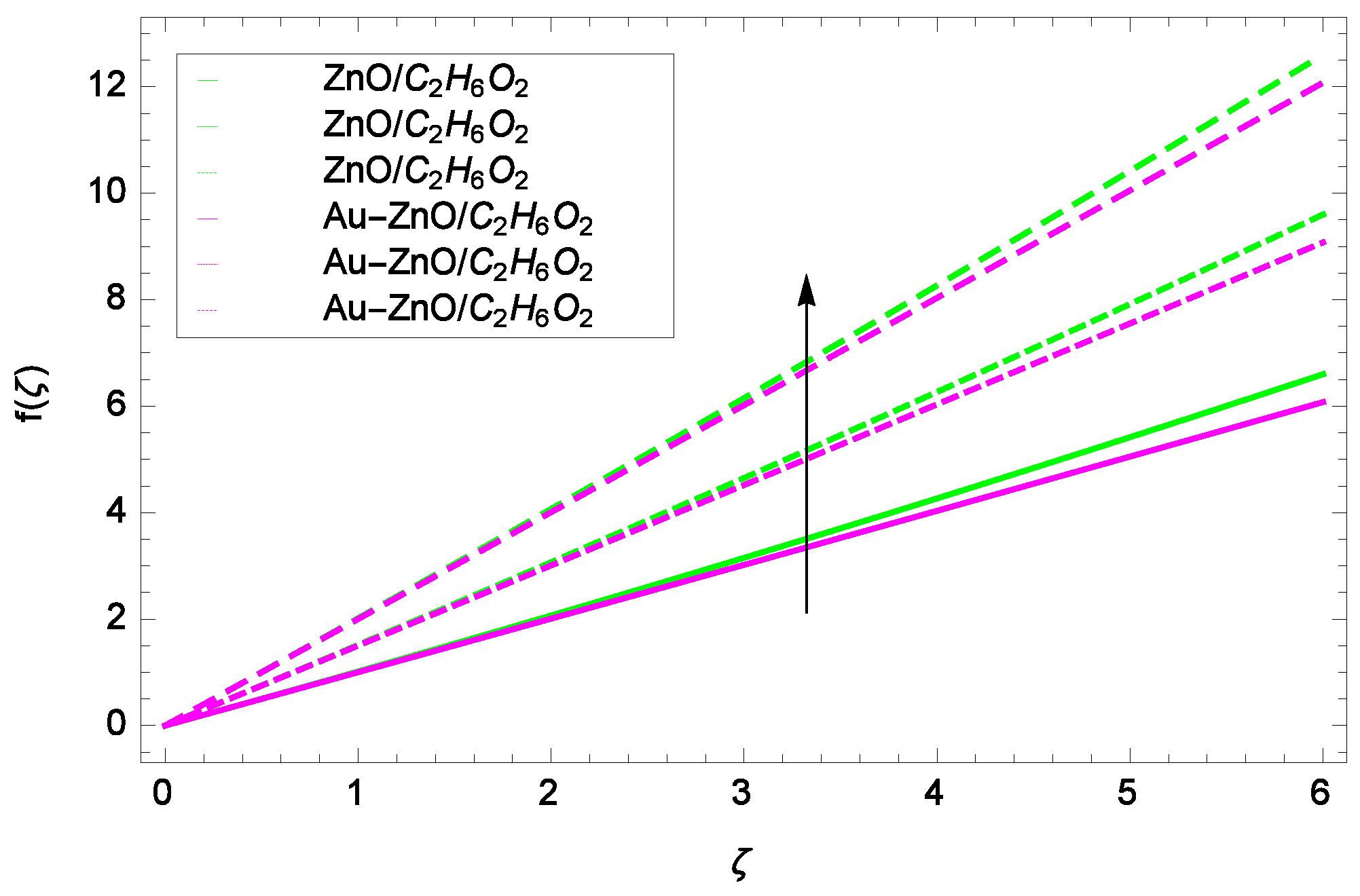
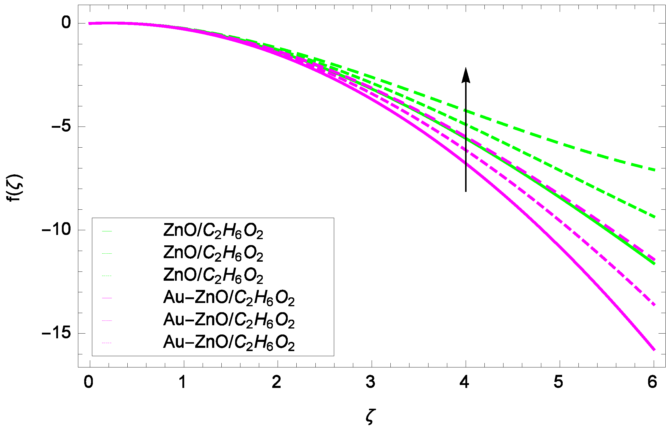
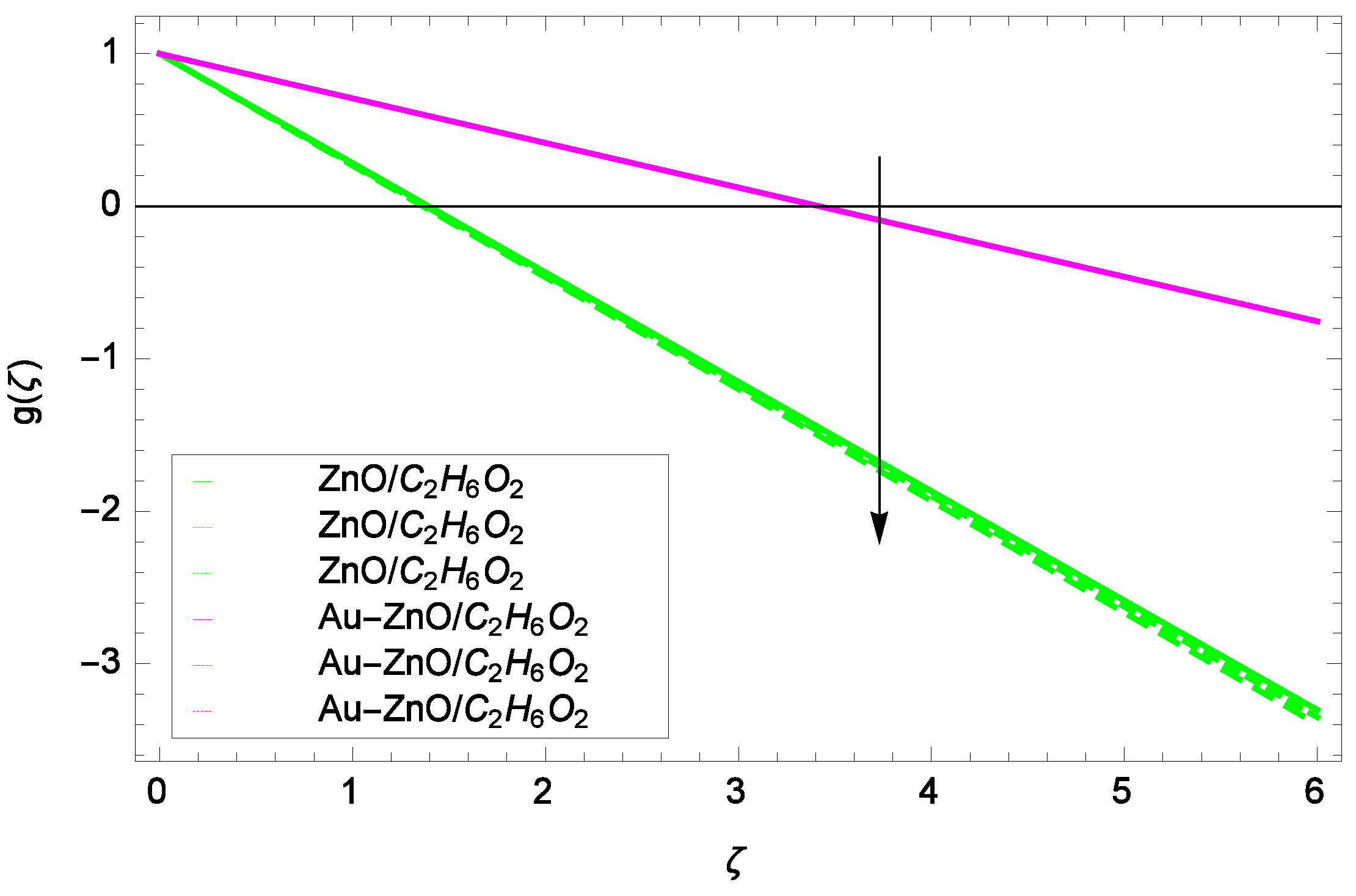
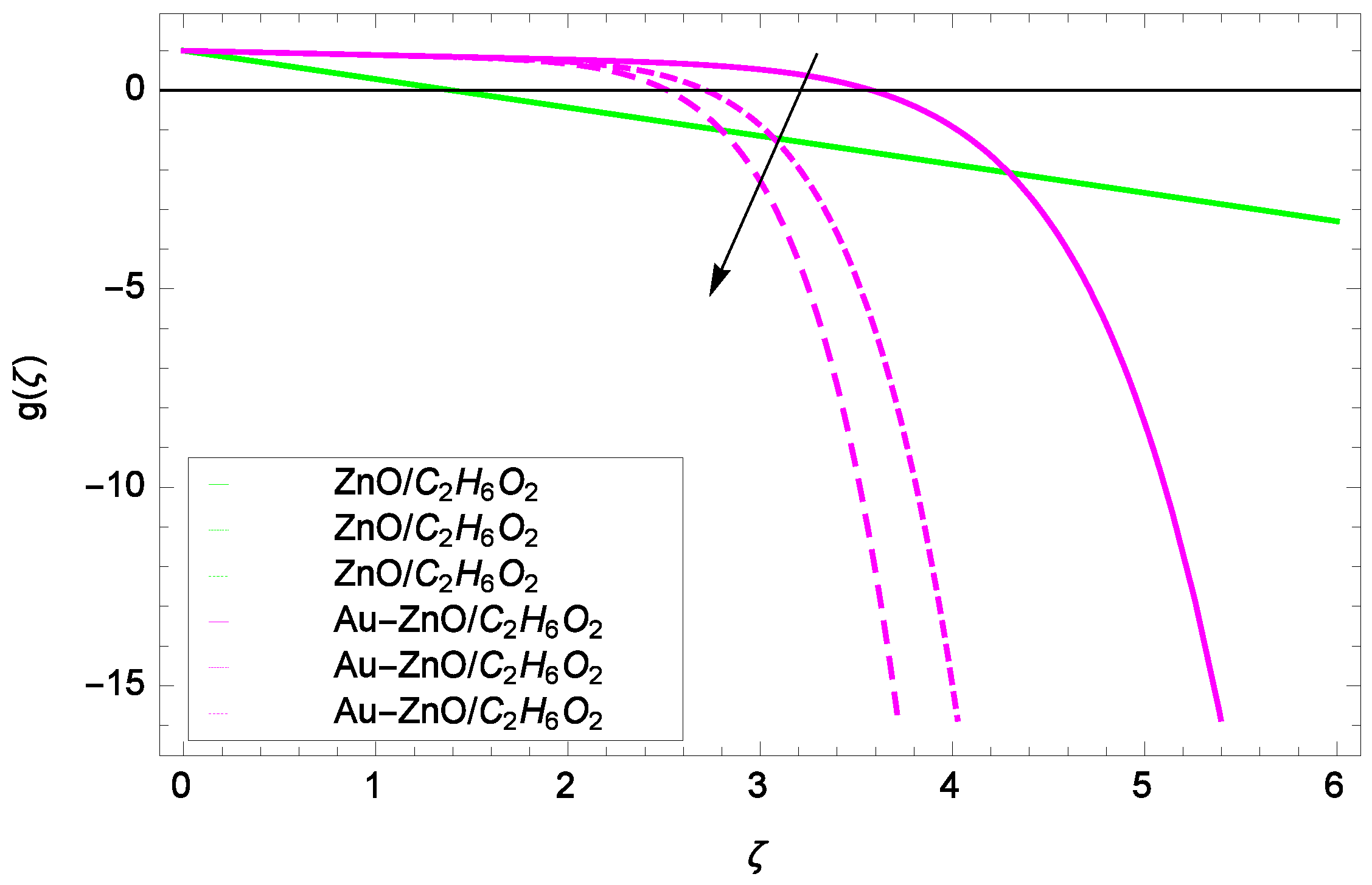
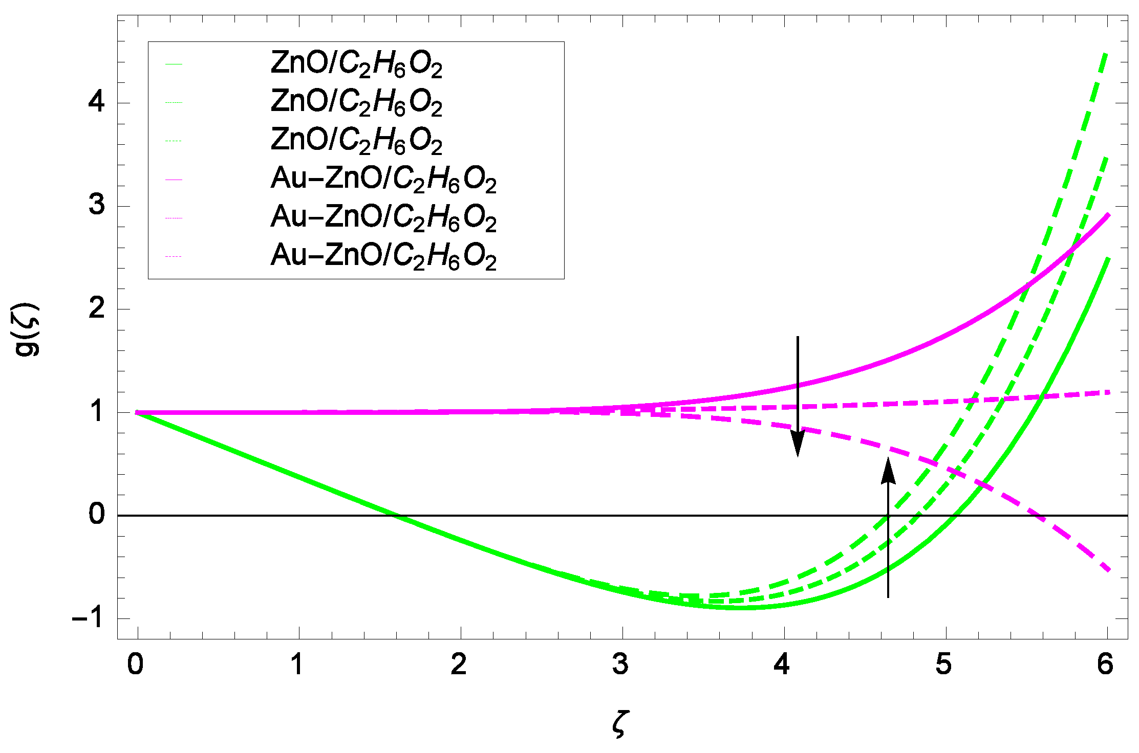
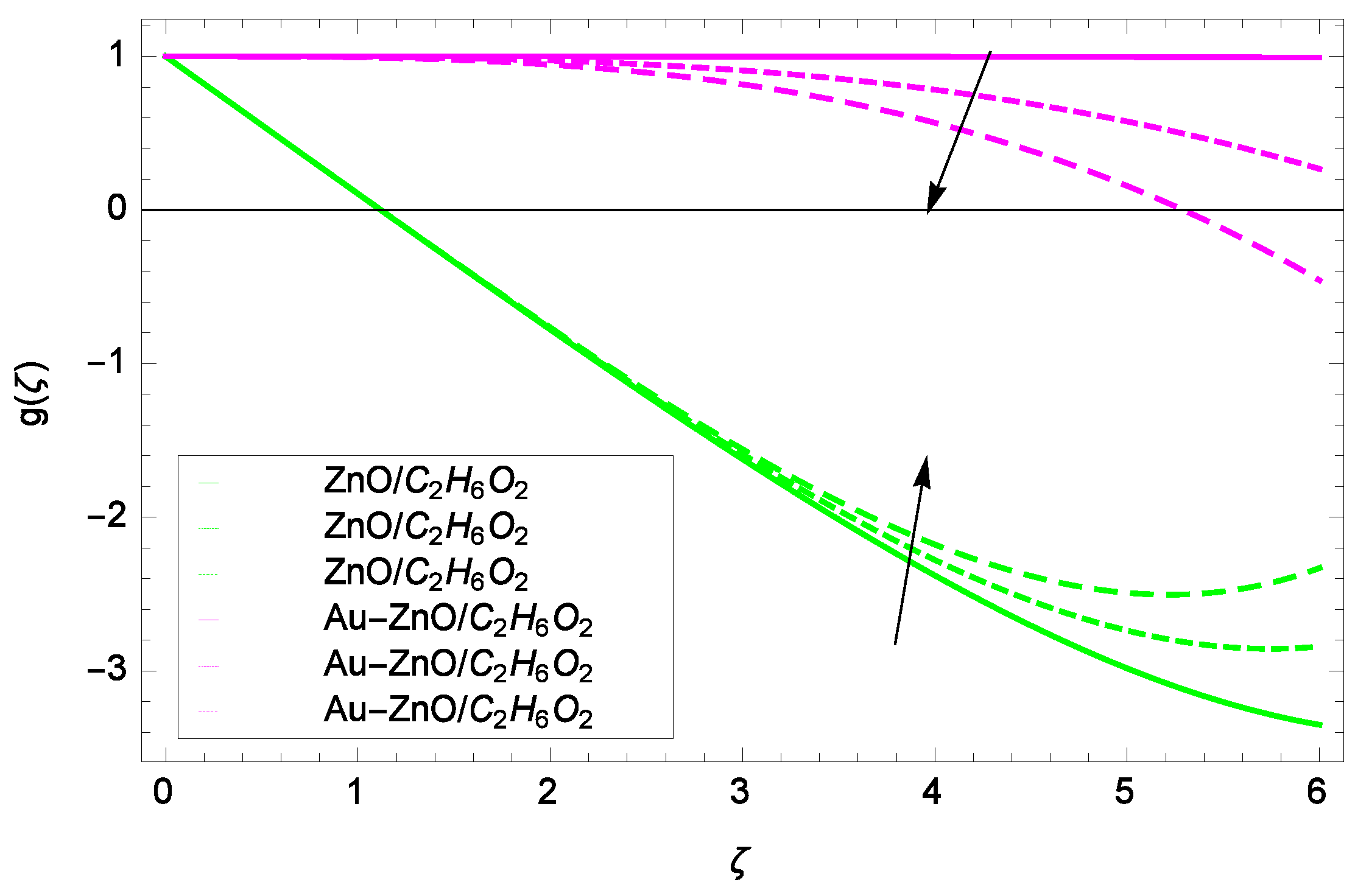
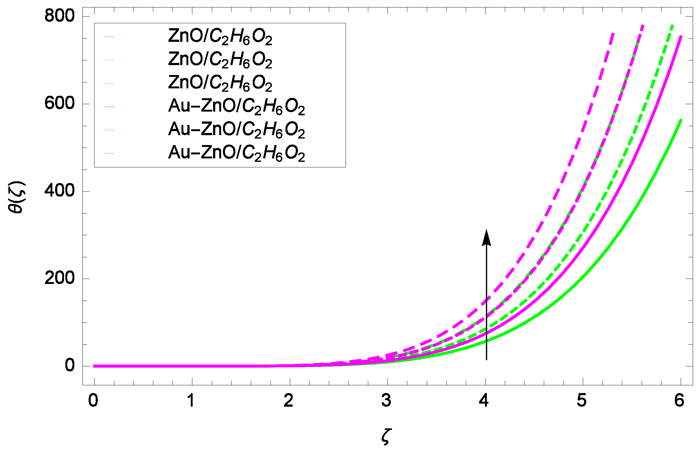
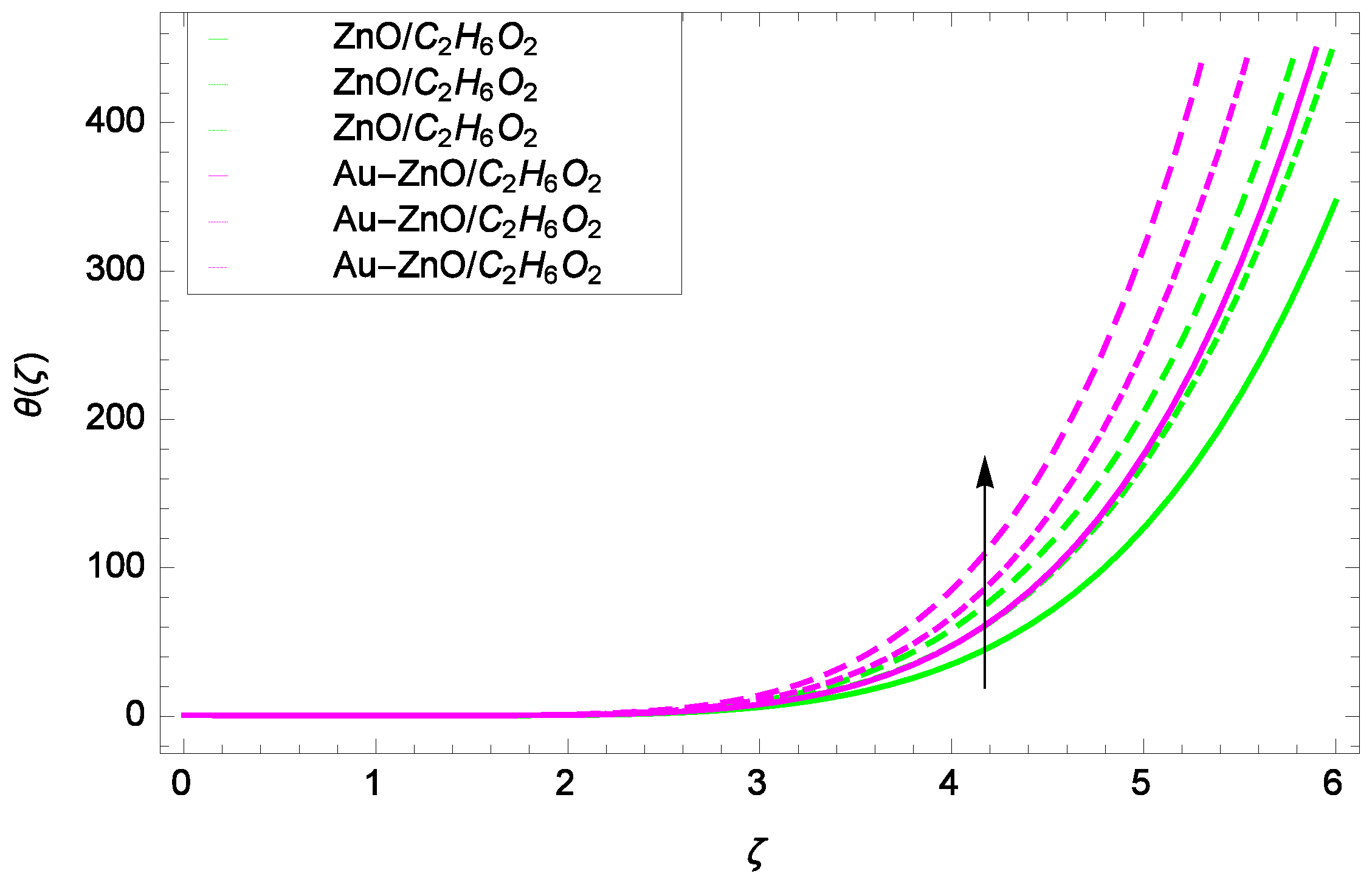
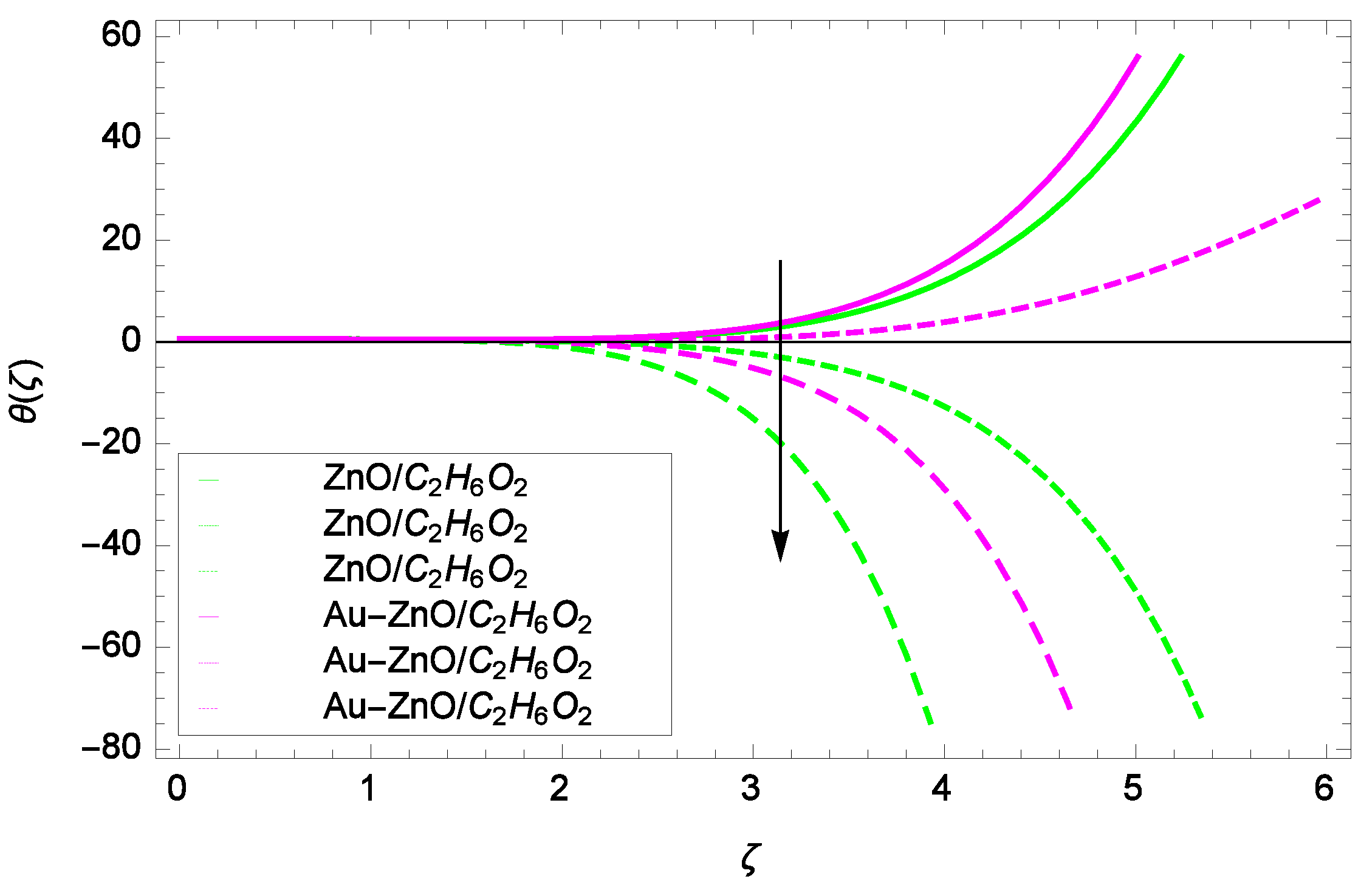
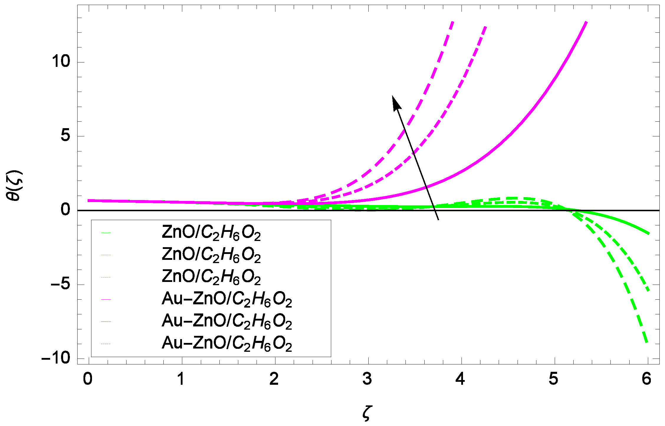
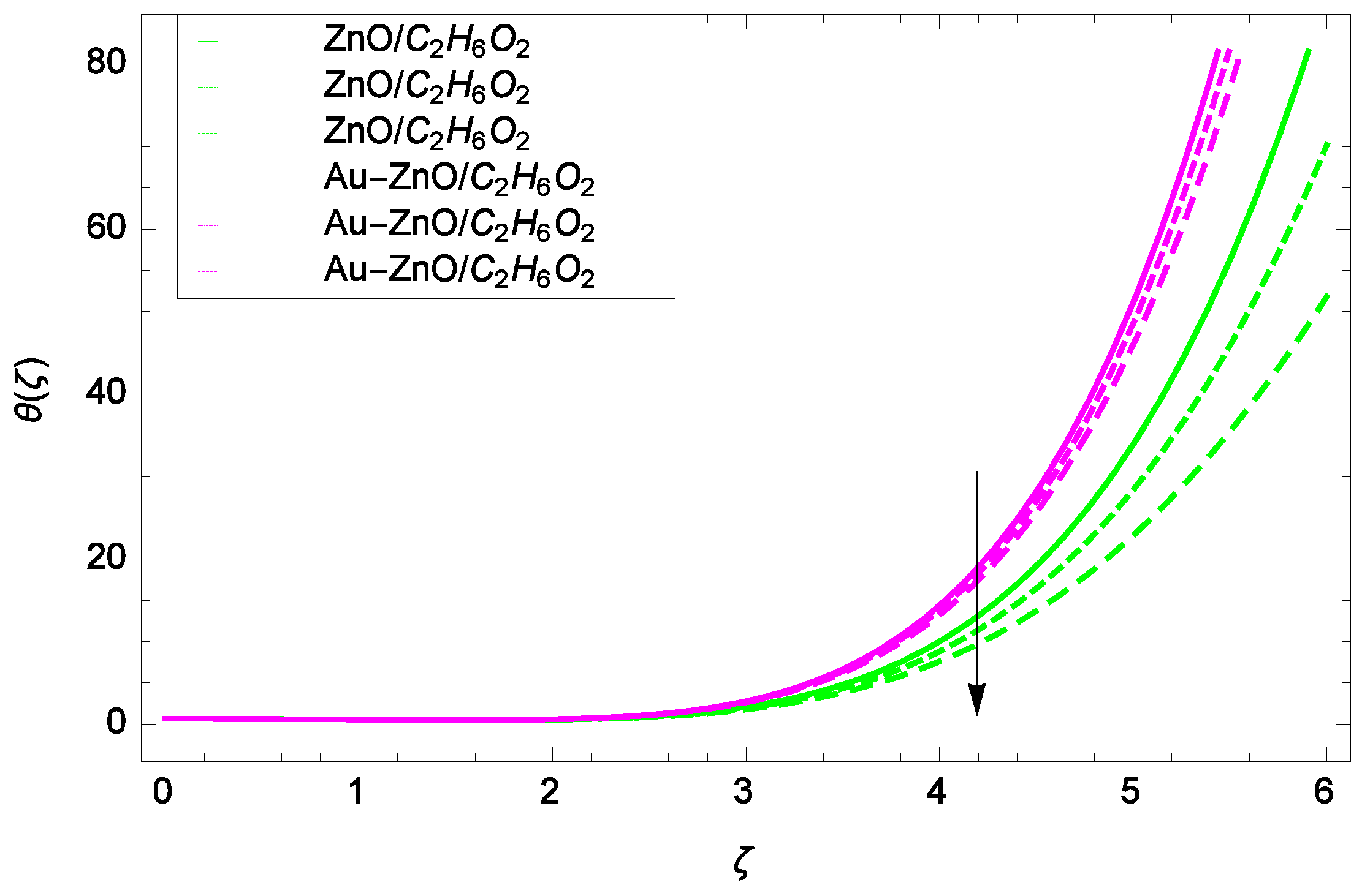
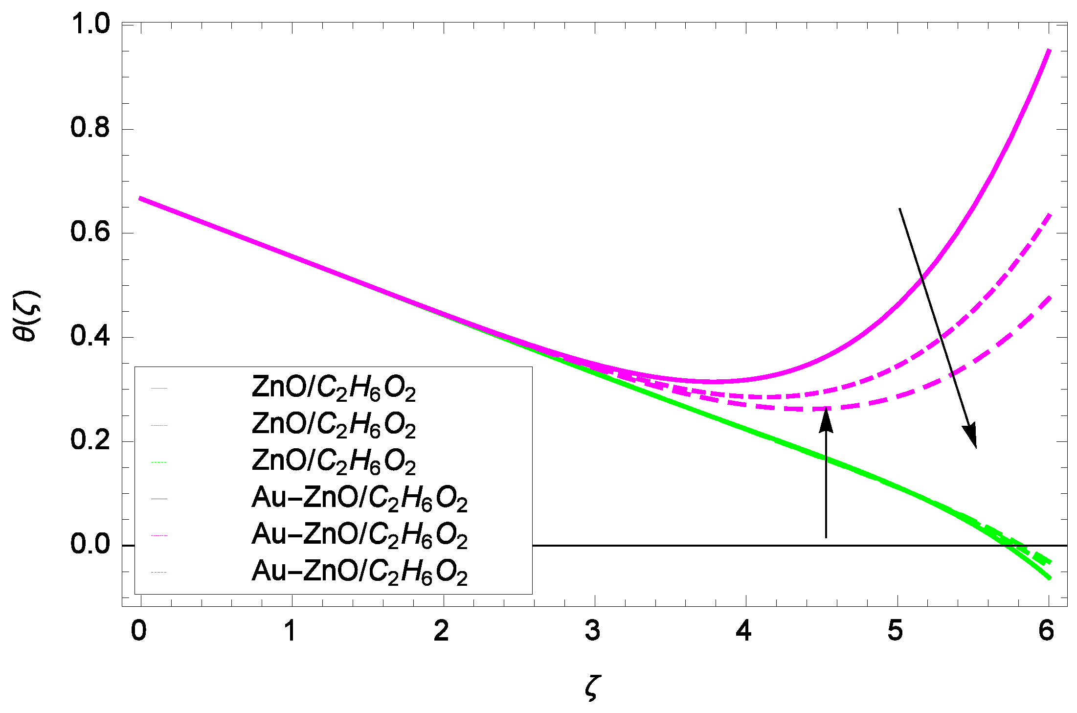
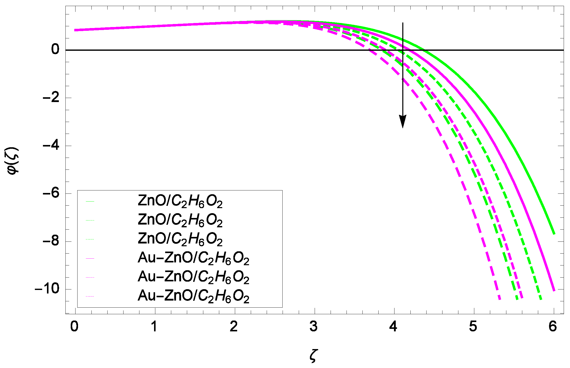
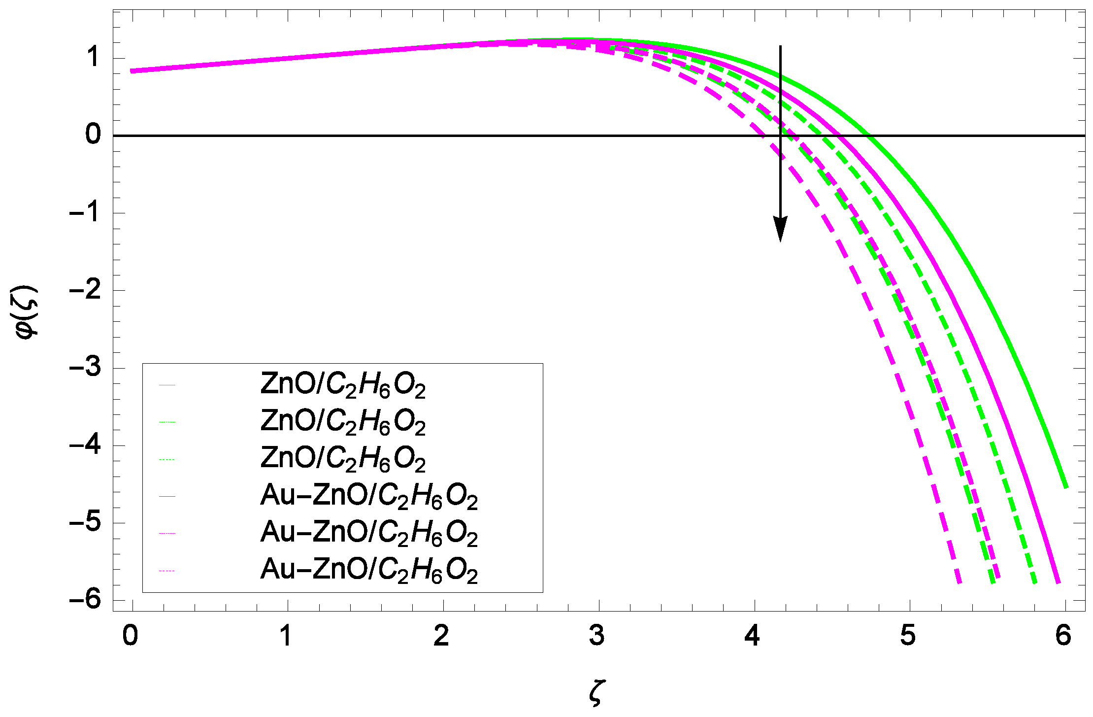
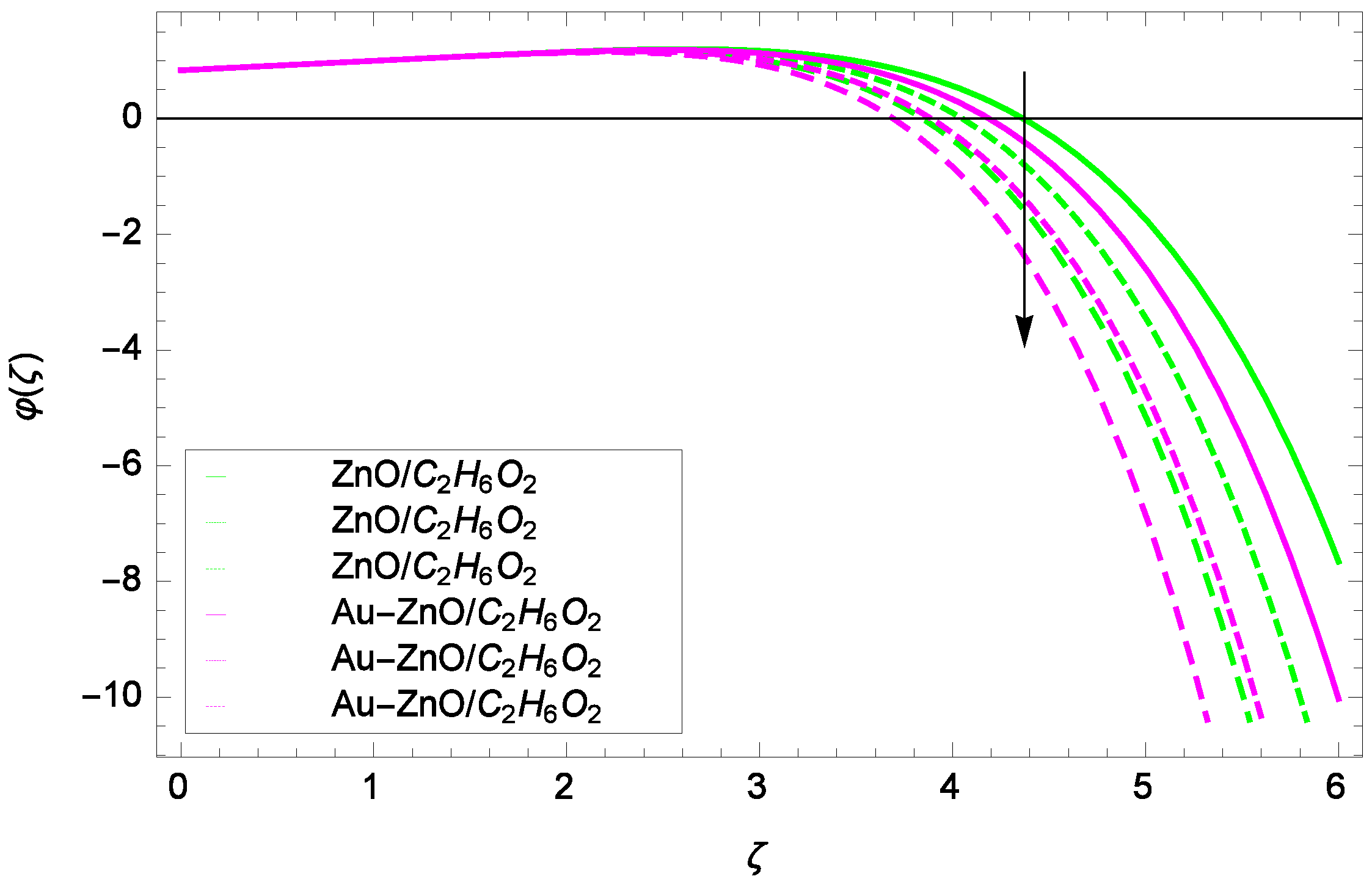
In the present study, two nanofluids namely ZnO-CHO and Au-ZnO/CHO are investigated whose behaviors are shown through the graphs under the effects of different parameters. In Figure 6, Figure 7, Figure 8, Figure 9, Figure 10, Figure 11, Figure 12, Figure 13, Figure 14, Figure 15, Figure 16, Figure 17, Figure 18, Figure 19, Figure 20, Figure 21, Figure 22, Figure 23, Figure 24 and Figure 25, the green and magenta colors are used for ZnO-CHO and Au-ZnO/CHO while in Figure 24 and Figure 25, the additional colors are also used. There are solid and dashed curves in Figure 6, Figure 7, Figure 8, Figure 9, Figure 10, Figure 11, Figure 12, Figure 13, Figure 14, Figure 15, Figure 16, Figure 17, Figure 18, Figure 19, Figure 20, Figure 21, Figure 22 and Figure 23. The mechanism is that three positive increasing numerical values are given to one parameter in the HAM solution while all the remaining parameters are fixed to show the effect of that one parameter simultaneously on the two nanofluids namely ZnO-CHO and Au-ZnO/CHO. When the solid lines locate below the dashed lines, then it shows the increasing effect and when the solid lines locate above the dashed lines, then it shows the decreasing effect. When the arrow head is from top to bottom, it shows the decreasing effect and when the arrow head is from bottom to top, it shows the increasing effect.
Figure 6 shows that for the different values of Reynolds number Re, the axial velocity f(ζ) is increased. In fact, the velocity of ZnO-CHO and Au-ZnO/CHO increase with increasing values of Reynolds number therefore overall motion is accelerated. Figure 7 shows the prominent role of stretching parameter k due to lower disk in which the axial velocity f(ζ) increases. The present motion is due to stretching so if the stretching parameter is increased, the flow of fluids is also increased. In the mean time, porosity is responsible to decrease the axial flow. It shows that motion due to different nanofluids is reduced because the permeability at the edge of the accelerating surface increases. Surely, it is noted that excess of nanoparticles concentration is involved in decelerating the motion. It is worthy of notice that the axial velocity f(ζ) decreases against the inertia. Physically it means that the absorbency of the porous medium shows an increment in the thickness of the fluid. Figure 8 shows that magnetic field parameter resists the flow since due to magnetic field, the Lorentz forces are generated which resist the motion. The curves are shrink in response to the parameter effect. Figure 9 exhibits all the assigned values of Ω and axial velocity f(ζ) which offers opportunities to know about the rotating systems and shows that the flow of ZnO-CHO and Au-ZnO/CHO increase.
Some interesting results have been found in case of tangential velocity g(ζ). Figure 10 shows that as the Reynolds number Re increases, the opposite tendency has been observed in the motion of ZnO-CHO and Au-ZnO/CHO. The flow of mono nanofluid ZnO-CHO decreases while the flow of hybrid nanofluid Au-ZnO/CHO shows no prominent change for increasing the Reynolds number Re. In Figure 11, the tangential velocity f(ζ) tends to decreasing. Tangential velocity assumes a likely downfall so the flow is not supported by stretching due to k. Figure 12 witnesses that the tangential velocity g(ζ) shifts to the effective decreasing for hybrid nanofluid Au-ZnO/CHO and increases for ZnO-CHO on behalf of the magnetic field parameter M. Figure 13 exhibits that rotation parameter Ω parameter resists the tangential flow of Au-ZnO/CHO and enhances the tangential flow of ZnO-CHO.
4.2. Temperature Profile
Figure 14 shows the effect of Reynolds number Re on heat transfer. The larger values of Re increase the temperature of ZnO-CHO and Au-ZnO/CHO. It has been observed in Figure 15 that as the stretching parameter k increases, the temperature of ZnO-CHO and Au-ZnO/CHO increase. These observations indicate that the fluid temperature and its related layer are incremented for higher estimations of k. The rotation parameter Ω cannot generate an extra heating to the system as shown in Figure 16. Temperature θ(ζ) is decreased on increasing the parameter Ω. The physical reason is that enhancement in Ω causes to improve the internal source of energy, that is why the fluid temperature is reduced. The system gets the parameter Pr for the designated values 1.00, 3.50, and 6.00 during the process and increases the temperature shown through Figure 17. The direct relation of Pr and thermal conductivity increases the thickness of thermal boundary layer. Larger values of Pr generate the high diffusion of heat transfer. The temperature θ(ζ) is changed to lowest level after the exchange of high values of magnetic field parameter M as shown in Figure 18. The reason is that strong Lorentz forces resist the flow of nanoparticles, so causing no high collision among the nanoparticles, consequently, the temperature is decreased. Figure 19 depicts that with the increasing values of thermal radiation parameter Rd, the temperature θ(ζ) of ZnO-CHO increases while the temperature of hybrid nanofluid Au-ZnO-CHO decreases. The reason is that radiation enhances more heat in the working fluids.
4.3. Concentration of Homogeneous-Heterogeneous Chemical Reactions
Looking at the non-dimensional Equation (28), the suitable values of Re, Sc and k are the basic quantities for generating a cubic autocatalysis chemical reaction. The concentration of chemical reaction φ(ζ) is low with the Reynolds number Re as shown in Figure 20. Figure 21 shows that for the homogeneous chemical reaction parameter k, the concentration of chemical reaction is decreased. From Equation (28), it is witnessed that the homogeneous chemical reaction parameter k is a part of performance with the multiple solutions. Enhancement in k makes dominant the concentration. In Figure 22, the stretching parameter k upgrades concentration of chemical reaction with low level by performing active role in the rotating motion. The stretching parameter k makes compact the homogeneous reaction and hence the concentration profile φ(ζ). Figure 23 stands for the outcomes of Schmidt number Sc and concentration φ(ζ). Momentum diffusivity to mass diffusivity is known as Schmidt number. The parameter Sc causes to make low the homogeneous chemical reaction.
4.4. Streamlines
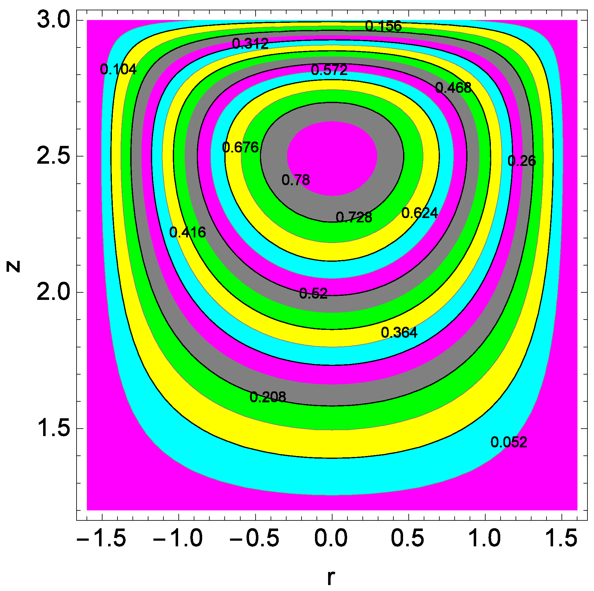
Figure 24 shows the streamlines at upper disks. The size of the streamlines increases at upper disk compared to that of lower disk. Both mono nanofluid and hybrid nanofluid proceed towards the edges of disks. Figure 25 shows the streamlines for the Reynolds number Re at lower disks. The compression of streamlines are clear from Figure 25. The plumes power is strong for lower disks.
4.5. Authentication of the Present Work
The important physical quantities introduced in Section 2 are evaluated to compare the validity of the solution with the published work [8]. Table 4 shows the tabulations to the several values for the parameter Re. There exists a nice agreement with the published work [8]. Similarly in Table 5, the values of heat transfer rate are computed for the volume fraction ϕ = 0.10, 0.20, 0.30, and 0.40. These values also have the close agreement with the published work [8].
5. Conclusions
A significant modification in the mathematical model for hybrid nanofluid has been made for the analysis of flow, heat and mass transfer. Chemical species reactions are shown in hybrid nanofluid. The problem is modeled in rotating systems for the nanoparticles ZnO and Au with base fluid ethylene glycol and solved through HAM. In ethylene glycol-based fluid (CHO), two types of nanoparticles, namely ZnO (zinc oxide) and Au (gold), with volume fractions = 0.03 and = 0.04 are investigated, respectively. It is noted that for = 0.00 and = 0.00, the problem becomes about viscous fluid with the absence of nanoparticles volume fractions. If = 0.00, Ag/CHO is obtained and if = 0.00, ZnO/CHO is constructed. Achieving better comprehension, the competencies of active parameters on flow, heat transfer and concentration of heterogeneous-homogeneous chemical reactions are noted. There exists a nice agreement between the present and published work in Table 4 and Table 5. The problem has potential for renewable energy system and researchers to investigate the thermal conductivity of nanoparticles like silver, aluminum, copper etc. with different base fluids like water, benzene, engine oil etc. The results for flow, heat transfer and concentration of homogeneous-heterogeneous chemical reactions are summarized as following.
- (1)
- Axial velocity f(ζ) increases for ZnO-CHO and Au-ZnO/CHO with the increasing values of Reynolds number Re, stretching parameter k and rotation parameter Ω while axial velocity f(ζ) decreases for ZnO-CHO and Au-ZnO/CHO with the increasing values of magnetic field parameter M.
- (2)
- Tangential velocity g(ζ) increases for ZnO-CHO with the increasing values of magnetic field parameter M and rotation parameter Ω while the same velocity decreases for Au-ZnO/CHO with the increasing values of magnetic field parameter M and rotation parameter Ω. Moreover, tangential velocity g(ζ) decreases for ZnO-CHO and Au-ZnO/CHO with the increasing values of Reynolds number Re and stretching parameter k.
- (3)
- Heat transfer increases for ZnO-CHO and Au-ZnO/CHO with the increasing values of Reynolds number Re, stretching parameter k. Similarly, heat transfer increases for ZnO-CHO with increasing values of thermal radiation parameter Rd while it is decreased for ZnO-CHO and Au-ZnO/CHO with the increasing values of rotation parameter Ω, magnetic field parameter M. In case of Au-ZnO/CHO, heat transfer also decreases with increasing values of thermal radiation parameter Rd.
- (4)
- The concentration of homogeneous-heterogeneous chemical reactions φ(ζ) decreases for ZnO-CHO and Au-ZnO/CHO with the increasing values of Reynolds number Re, stretching parameter k and Schmidt number Sc.
- (5)
- Streamlines are compressed at the upper portion of upper disk while these are compressed at the lower portion of lower disk when the Reynolds number Re assumes the value 0.30.
- (6)
Author Contributions
Conceptualization, N.S.K.; methodology, N.S.K.; software, N.S.K.; validation, N.S.K.; formal analysis, P.K.; investigation, N.S.K.; resources, P.T.; data curation, P.T.; writing—original draft preparation, N.S.K.; writing—review and editing, N.S.K.; visualization, P.K.; supervision, N.S.K.; project administration, P.K.; funding acquisition, P.K. All authors have read and agreed to the revised version of the manuscript.
Funding
This research is funded by the Center of Excellence in Theoretical and Computational Science (TaCS-CoE), KMUTT.
Acknowledgments
This work was partially supported by the International Research Partnerships: Electrical Engineering Thai-French Research Center (EE-TFRC) between King Mongkut’s University of Technology North Bangkok and Universite’ de Lorraine under Grant KMUTNB-BasicR-64-17. The authors are cordially thankful to the honorable reviewers for their constructive comments to improve the quality of the paper. This research is supported by the Postdoctoral Fellowship from King Mongkut’s University of Technology Thonburi (KMUTT), Thailand. This project is supported by the Theoretical and Computational Science (TaCS) Center under Computational and Applied Science for Smart Innovation Research Cluster (CLASSIC), Faculty of Science, KMUTT.
Conflicts of Interest
The authors declare no conflict of interest.
References
- Kasaeian, A.; Eshghi, A.T.; Sameti, M. A review on the applications of nanofluids in solar energy systems. Renew. Sustain. Energy Rev. 2015, 43, 584–598. [Google Scholar] [CrossRef]
- Ettefaghi, E.; Ghobadian, B.; Rashidi, S.; Najafi, G.; Khoshtaghaza, M.H.; Rashtchi, M.; Sadeghian, S. A novel bio-nano emulsion fuel based on biodegradable nanoparticles to improve diesel engines performance and reduce exhaust emissions. Renew. Energy 2018, 125, 64–72. [Google Scholar] [CrossRef]
- Gunjo, D.G.; Jena, S.R.; Mahanta, P.; Robi, P.S. Melting enhancement of a latent heat storage with dispersed Cu, CuO and Al2O3 nanoparticles for solar thermal application. Renew. Energy 2018, 121, 652–665. [Google Scholar] [CrossRef]
- Khanafer, K.; Vafi, K. A review on the aplications of nanofluids in solar energy field. Renew. Energy 2018, 123, 398–406. [Google Scholar] [CrossRef]
- Caglar, M.; Ilican, S.; Caglar, Y.; Yakuphanoglu, F. Electrical conductivity and optical properties of Zno nanostructured thin film. Appl. Surf. Sci. 2009, 225, 4491–4496. [Google Scholar] [CrossRef]
- Islam, R.I.; Shabani, B.; Rosengarten, G. Electrical and thermal conductivities of water-ethylene glycol based TiO2 nanofluids to be used as coolants in PEM fuel cells. Energy Procedia 2017, 110, 101–108. [Google Scholar] [CrossRef]
- Fal, J.; Sidorowicz, A.; Zyla, G. Electrical conductivity of ethylene glycol based nanofluids with different types of thulium oxide nanoparticles. Acta Phys. Pol. A 2017, 132, 146–148. [Google Scholar] [CrossRef]
- Rout, B.C.; Mishra, S.R.; Nayak, B. Semi analytical solution of axisymmetric flows of Cu- and Ag-water nanofluids between two rotating disks. Heat Transf. Asian Res. 2019, 132, 1–25. [Google Scholar] [CrossRef]
- Hamilton, R.L.; Crosser, O.K. Thermal conductivity of heterogeneous two component systems. Ind. Eng. Chem. Fundam. 1962, 1, 187–191. [Google Scholar] [CrossRef]
- Choi, S.U.S.; Eastman, J.A. Enhancing thermal conductivity of fluids with nanoparticles. In Proceedings of the 1995 International Mechanical Engineering Congress and Exhibition, San Francisco, CA, USA, 12–17 November 1995; Volume 231, pp. 99–106. [Google Scholar]
- Vallejo, J.P.; Zyla, G.; Fernandez-Seara, J.; Lugo, L. Influence of six carbon-based nanomaterials on the rheological properties of nanofluids. Nanomaterials 2019, 9, 146. [Google Scholar] [CrossRef] [Green Version]
- Alihosseini, S.; Jafari, A. The effect of porous medium configuration on nanofluid heat transfer. Appl. Nanosci. 2020, 10, 895–906. [Google Scholar] [CrossRef]
- Sheikholeslami, M.; Shah, Z.; Tassaddiq, A.; Shafee, A.; Khan, I. Application of electric field for augmentation of Ferrofluid heat transfer in an enclosure including double moving walls. IEEE Access 2019, 7, 21048–21056. [Google Scholar] [CrossRef]
- Al-Kouz, W.; Al-Muhtady, A.; Owhaib, W.; Al-Dahidi, S.; Hadar, M.; Abu-Alghanam, R. Entropy generation optimization for rarified nanofluid flows in a square cavity with two fins at the hot wall. Entropy 2019, 21, 103. [Google Scholar] [CrossRef] [Green Version]
- Atta, A.M.; Abdullah, M.M.S.; Al-Lohedan, H.A.; Mohamed, N.H. Novel superhydrophobic sand and polyurethane sponge coated with silica/modified asphaltene nanoparticles for rapid oil spill cleanup. Nanomaterials 2019, 9, 187. [Google Scholar] [CrossRef] [Green Version]
- Rout, A.; Boltaev, G.S.; Ganeev, R.A.; Fu, Y.; Maurya, S.K.; Kim, V.V.; Rao, K.S.; Guo, C. Nonlinear optical studies of gold nanoparticles films. Nanomaterials 2019, 9, 291. [Google Scholar] [CrossRef] [PubMed] [Green Version]
- Alvarez-Regueiro, E.; Vallejo, J.P.; Fernandez-Seara, J.; Fernandez, J.; Lugo, L. Experimental convection heat transfer analysis of a nano-enhanced industrial coolant. Nanomaterials 2019, 9, 267. [Google Scholar] [CrossRef] [Green Version]
- Alsagri, A.S.; Nasir, S.; Gul, T.; Islam, S.; Nisar, K.S.; Shah, Z.; Khan, I. MHD thin film flow and thermal analysis of blood with CNTs nanofluid. Coatings 2019, 9, 175. [Google Scholar] [CrossRef] [Green Version]
- Mishra, S.K.; Chandra, H.; Arora, A. Effect of velocity and rheology of nanofluid on heat transfer of laminar vibrational flow through a pipe under constant heat flux. Int. Nano Lett. 2019, 9, 245–256. [Google Scholar] [CrossRef] [Green Version]
- Abbas, S.Z.; Khan, W.A.; Sun, H.; Ali, M.; Irfan, M.; Shahzed, M.; Sultan, F. Mathematical modeling and analysis of cross nanofluid flow subjected to entropy generation. Appl. Nanosci. 2019, 10, 3149–3160. [Google Scholar] [CrossRef]
- Ali, M.; Khan, W.A.; Irfan, M.; Sultan, F.; Shahzed, M.; Khan, M. Computational analysis of entropy generation for cross nanofluid flow. Appl. Nanosci. 2019, 10, 3045–3055. [Google Scholar] [CrossRef]
- Sharma, R.P.; Seshadri, R.; Mishra, S.R.; Munjam, S.R. Effect of thermal radiation on magnetohydrodynamic three-dimensional motion of a nanofluid past a shrinking surface under the influence of a heat source. Heat Transf. Asian Res. 2019, 48, 2105–2121. [Google Scholar] [CrossRef]
- Jahan, S.; Sakidin, H.; Nazar, R.; Pop, I. Analysis of heat transfer in nanofluid past a convectively heated permeable stretching/shrinking sheet with regression and stability analyses. Results Phys. 2018, 10, 395–405. [Google Scholar] [CrossRef]
- Hossinzadeh, K.; Asadi, A.; Mogharrebi, A.R.; Khalesi, J.; Mousavisani, S.; Ganji, D.D. Entropy generation analysis of (CH2OH)2 containing CNTs nanofluid flow under effect of MHD and thermal radiation. Case Stud. Therm. Eng. 2019, 14, 100482. [Google Scholar] [CrossRef]
- Khan, N.S. Bioconvection in second grade nanofluid flow containing nanoparticles and gyrotactic microorganisms. Braz. J. Phys. 2018, 43, 227–241. [Google Scholar] [CrossRef]
- Khan, N.S.; Gul, T.; Khan, M.A.; Bonyah, E.; Islam, S. Mixed convection in gravity-driven thin film non-Newtonian nanofluids flow with gyrotactic microorganisms. Results Phys. 2017, 7, 4033–4049. [Google Scholar] [CrossRef]
- Khan, N.S.; Gul, T.; Islam, S.; Khan, I.; Alqahtani, A.M.; Alshomrani, A.S. Magnetohydrodynamic nanoliquid thin film sprayed on a stretching cylinder with heat transfer. J. Appl. Sci. 2017, 7, 271. [Google Scholar] [CrossRef]
- Zuhra, S.; Khan, N.S.; Khan, M.A.; Islam, S.; Khan, W.; Bonyah, E. Flow and heat transfer in water based liquid film fluids dispensed with graphene nanoparticles. Results Phys. 2018, 8, 1143–1157. [Google Scholar] [CrossRef]
- Khan, N.S.; Gul, T.; Islam, S.; Khan, W. Thermophoresis and thermal radiation with heat and mass transfer in a magnetohydrodynamic thin film second-grade fluid of variable properties past a stretching sheet. Eur. Phys. J. Plus 2017, 132, 11. [Google Scholar] [CrossRef]
- Palwasha, Z.; Khan, N.S.; Shah, Z.; Islam, S.; Bonyah, E. Study of two dimensional boundary layer thin film fluid flow with variable thermo-physical properties in three dimensions space. AIP Adv. 2018, 8, 105318. [Google Scholar] [CrossRef] [Green Version]
- Khan, N.S.; Gul, T.; Islam, S.; Khan, A.; Shah, Z. Brownian motion and thermophoresis effects on MHD mixed convective thin film second-grade nanofluid flow with Hall effect and heat transfer past a stretching sheet. J. Nanofluids 2017, 6, 812–829. [Google Scholar] [CrossRef]
- Khan, N.S.; Zuhra, S.; Shah, Z.; Bonyah, E.; Khan, W.; Islam, S. Slip flow of Eyring-Powell nanoliquid film containing graphene nanoparticles. AIP Adv. 2019, 8, 115302. [Google Scholar] [CrossRef]
- Khan, N.S.; Gul, T.; Kumam, P.; Shah, Z.; Islam, S.; Khan, W.; Zuhra, S.; Sohail, A. Influence of inclined magnetic field on Carreau nanoliquid thin film flow and heat transfer with graphene nanoparticles. Energies 2019, 12, 1459. [Google Scholar] [CrossRef] [Green Version]
- Khan, N.S. Study of two dimensional boundary layer flow of a thin film second grade fluid with variable thermo-physical properties in three dimensions space. Filomat 2019, 33, 5387–5405. [Google Scholar] [CrossRef] [Green Version]
- Khan, N.S.; Zuhra, S. Boundary layer unsteady flow and heat transfer in a second grade thin film nanoliquid embedded with graphene nanoparticles past a stretching sheet. Adv. Mech. Eng. 2019, 11, 1–11. [Google Scholar] [CrossRef] [Green Version]
- Khan, N.S.; Gul, T.; Islam, S.; Khan, W.; Khan, I.; Ali, L. Thin film flow of a second-grade fluid in a porous medium past a stretching sheet with heat transfer. Alex. Eng. J. 2017, 57, 1019–1031. [Google Scholar] [CrossRef]
- Zuhra, S.; Khan, N.S.; Alam, A.; Islam, S.; Khan, A. Buoyancy effects on nanoliquids film flow through a porous medium with gyrotactic microorganisms and cubic autocatalysis chemical reaction. Adv. Mech. Eng. 2020, 12, 1–17. [Google Scholar] [CrossRef] [Green Version]
- Palwasha, Z.; Islam, S.; Khan, N.S.; Ayaz, H. Non-Newtonian nanoliquids thin film flow through a porous medium with magnetotactic microorganisms. Appl. Nanosci. 2018, 8, 1523–1544. [Google Scholar] [CrossRef]
- Khan, N.S. Mixed convection in MHD second grade nanofluid flow through a porous medium containing nanoparticles and gyrotactic microorganisms with chemical reaction. Filomat 2019, 33, 4627–4653. [Google Scholar] [CrossRef] [Green Version]
- Zuhra, S.; Khan, N.S.; Shah, Z.; Islam, Z.; Bonyah, E. Simulation of bioconvection in the suspension of second grade nanofluid containing nanoparticles and gyrotactic microorganisms. AIP Adv. 2018, 8, 105210. [Google Scholar] [CrossRef] [Green Version]
- Khan, N.S.; Shah, Z.; Shutaywi, M.; Kumam, P.; Thounthong, P. A comprehensive study to the assessment of Arrhenius activation energy and binary chemical reaction in swirling flow. Sci. Rep. 2020, 10, 7868. [Google Scholar] [CrossRef]
- Zuhra, S.; Khan, N.S.; Islam, S. Magnetohydrodynamic second grade nanofluid flow containing nanoparticles and gyrotactic microorganisms. Comput. Appl. Math. 2018, 37, 6332–6358. [Google Scholar] [CrossRef]
- Zuhra, S.; Khan, N.S.; Islam, S.; Nawaz, R. Complexiton solutions for complex KdV equation by optimal homotopy asymptotic method. Filomat 2020, 33, 6195–6211. [Google Scholar] [CrossRef]
- Zahra, A.; Mahanthesh, B.; Basir, M.F.M.; Imtiaz, M.; Mackolil, J.; Khan, N.S.; Nabwey, H.A.; Tlili, I. Mixed radiated magneto Casson fluid flow with Arrhenius activation energy and Newtonian heating effects: Flow and sensitivity analysis. Alex. Eng. J. 2020, 57, 1019–1031. [Google Scholar]
- Liaqat, A.; Asifa, T.; Ali, R.; Islam, S.; Gul, T.; Kumam, P.; Mukhtar, S.; Khan, N.S.; Thounthong, P. A new analytical approach for the research of thin-film flow of magneto hydrodynamic fluid in the presence of thermal conductivity and variable viscosity. ZAMM J. Appl. Math. Mech. Z. Angewwandte Math. Mech. 2020, 1–13. [Google Scholar] [CrossRef]
- Khan, N.S.; Zuhra, S.; Shah, Q. Entropy generation in two phase model for simulating flow and heat transfer of carbon nanotubes between rotating stretchable disks with cubic autocatalysis chemical reaction. Appl. Nanosci. 2019, 9, 1797–1822. [Google Scholar] [CrossRef]
- Khan, N.S.; Shah, Z.; Islam, S.; Khan, I.; Alkanhal, T.A.; Tlili, I. Entropy generation in MHD mixed convection non-Newtonian second-grade nanoliquid thin film flow through a porous medium with chemical reaction and stratification. Entropy 2019, 21, 139. [Google Scholar] [CrossRef] [Green Version]
- Khan, N.S.; Zuhra, S.; Shah, Z.; Bonyah, E.; Khan, W.; Islam, S.; Khan, A. Hall current and thermophoresis effects on magnetohydrodynamic mixed convective heat and mass transfer thin film flow. J. Phys. Commun. 2019, 3, 035009. [Google Scholar] [CrossRef]
- Khan, N.S.; Kumam, P.; Thounthong, P. Renewable energy technology for the sustainable development of thermal system with entropy measures. Int. J. Heat Mass Transf. 2019, 145, 118713. [Google Scholar] [CrossRef]
- Khan, N.S.; Kumam, P.; Thounthong, P. Second law analysis with effects of Arrhenius activation energy and binary chemical reaction on nanofluid flow. Sci. Rep. 2020, 10, 1226. [Google Scholar] [CrossRef] [Green Version]
- Khan, N.S.; Shah, Q.; Bhaumik, A.; Kumam, P.; Thounthong, P.; Amiri, I. Entropy generation in bioconvection nanofluid flow between two stretchable rotating disks. Sci. Rep. 2020, 10, 4448. [Google Scholar] [CrossRef]
- Khan, N.S.; Shah, Q.; Sohail, A. Dynamics with Cattaneo-Christov heat and mass flux theory of bioconvection Oldroyd-B nanofluid. Adv. Mech. Eng. 2020. [Google Scholar] [CrossRef]
- Khan, N.S.; Shah, Q.; Sohail, A.; Kumam, P.; Thounthong, P.; Bhaumik, A.; Ullah, Z. Lorentz forces effects on the interactions of nanoparticles in emerging mechanisms with innovative approach. Symmetry 2020, 5, 1700. [Google Scholar] [CrossRef]
- Liaqat, A.; Khan, N.S.; Ali, R.; Islam, S.; Kumam, P.; Thounthong, P. Novel insights through the computational techniques in unsteady MHD second grade fluid dynamics with oscillatory boundary conditions. Heat Transf. 2020. [Google Scholar] [CrossRef]
- Khan, N.S.; Ali, L.; Ali, R.; Kumam, P.; Thounthong, P. A novel algorithm for the computation of systems containing different types of integral and integro-differential equations. Heat Transf. 2020. [Google Scholar] [CrossRef]
- Ahmad, S.; Nadeem, S.; Ullah, N. Entropy generation and temperature-dependent viscosity in the study of SWCNT-MWCNT hybrid nanofluid. Appl. Nanosci. 2020. [Google Scholar] [CrossRef]
- Dinarvand, S.; Rostami, M.N. An innovative mass-based model of aqueous zinc oxide-gold hybrid nanofluid for von Karman’s swirling flow. J. Therm. Anal. Calorim. 2019, 138, 845–855. [Google Scholar] [CrossRef]
- Ahmed, S.; Xu, H. Mixed convection in gravity driven thin nano-liquid film flow with homogeneous-heterogeneous reactions. Phys. Fluids 2020, 32, 023604. [Google Scholar] [CrossRef]
- Hayat, T.; Haider, F.; Muhammad, T.; Ahmad, B. Darcy-Forchheimer flow of carbon nanotubes due to a convectively heated rotating disk with homogeneous-heterogeneous chemical reactions. J. Therm. Anal. Calorim. 2019, 137, 1939–1949. [Google Scholar] [CrossRef]
- Suleman, M.; Ramzan, M.; Ahmad, S.; Lu, D.; Muhammad, T.; Chung, J.D. A numerical simulation of silver-water nanofluid flow with impacts of Newtonian heating and homogeneous-heterogeneous reactions past a nonlinear stretched cylinder. Symmetry 2019, 11, 295. [Google Scholar] [CrossRef] [Green Version]
- Liao, S.J. Homotopy Analysis Method in Non-Linear Differential Equations; Higher Education Press: Beijing, China; Springer: Berlin/Heidelberg, Germany, 2012. [Google Scholar]
Figure 1.
Geometry of the problem.

Figure 2.
Illustration of the -curve of f(ζ).

Figure 3.
Illustration of the -curve of g(ζ).

Figure 4.
Illustration of the -curve of θ(ζ).

Figure 5.
Illustration of the -curve of φ(ζ).

Figure 6.
Illustration for the velocity f(ζ) and parameter Re = 1.00, 1.50, 2.00.

Figure 7.
Illustration for the velocity f(ζ) and parameter k = 1.00, 1.50, 2.00.

Figure 8.
Illustration for the velocity f(ζ) and parameter M = 1.00, 1.50, 2.00.

Figure 9.
Illustration for the velocity f(ζ) and parameter Ω = 1.00, 1.50, 2.00.

Figure 10.
Illustration for the velocity g(ζ) and parameter Re = 1.00, 10.50, 20.00.

Figure 11.
Illustration for the velocity g(ζ) and parameter k = 1.00, 10.50, 20.00.

Figure 12.
Illustration for the velocity g(ζ) and parameter M = 1.00, 10.50, 20.00.

Figure 13.
Illustration for the velocity g(ζ) and parameter Ω = 1.00, 1.50, 2.00.

Figure 14.
Illustration for the heat transfer θ(ζ) and parameter Re = 1.00, 1.50, 2.00.

Figure 15.
Illustration for the heat transfer θ(ζ) and parameter k = 1.00, 1.50, 2.00.

Figure 16.
Illustration for the heat transfer θ(ζ) and parameter Ω = 1.00, 5.50, 10.00.

Figure 17.
Illustration for the heat transfer θ(ζ) and parameter Pr = 1.00, 3.50, 6.00.

Figure 18.
Illustration for the heat transfer θ(ζ) and parameter M = 1.00, 1.50, 2.00.

Figure 19.
Illustration for the heat transfer θ(ζ) and parameter Rd = 1.00, 1.50, 2.00.

Figure 20.
Illustration for the concentration φ(ζ) and parameter Re = 1.00, 1.50, 2.00.

Figure 21.
Illustration for the concentration φ(ζ) and parameter k = 1.00, 1.50, 2.00.

Figure 22.
Illustration for the concentration φ(ζ) and parameter k = 1.00, 1.50, 2.00.

Figure 23.
Illustration for the concentration φ(ζ) and parameter Sc = 1.00, 1.50, 2.00.

Figure 24.
Illustration for the streamlines at upper disk and parameter Re = 0.30.

Figure 25.
Illustration for the streamlines for lower disks and parameter Re = 0.30.


Table 1.
Values of shape factor of different shapes of nanoparticles.
| Shapes of Nanoparticle | n | Aspect Ratio |
|---|---|---|
| Spherical | 3 | - |
| Brick | 3.7 | 1:1:1 |
| Cylinder | 4.8 | 1:8 |
| Platelet | 5.7 | 1:1/8 |
Table 2.
Thermophysical properties of ethylene glycol and nanoparticles.
| Properties | Ethylene Glycol (CHO) | Zinc Oxide (ZnO) | Gold (Au) |
|---|---|---|---|
| (kg/m) | = 116.6 | = 5600 | = 19,282 |
| c(J/kg K) | (c) = 2382 | (c) = 495.2 | (c) = 192 |
| k(W/m K) | k = 0.249 | k = 13 | k = 310 |
| (Um) | = 3.14 | = 7.261 × 10 | = 4.11 × 10 |
| Nanoparticle measurement/nm | - | 29 and 77 | 3–40 |
Table 3.
Mathematical forms of thermophysical properties.
| Properties | ZnO/CHO |
|---|---|
| Density () | = (1 − ) + |
| Heat capacity (c) | (c) = (1 − )(c) + (c) |
| Dynamic viscosity () | = |
| Thermal conductivity (k) | = |
| Electrical conductivity () | = 1 + , where = |
| Properties | Hybrid nanofluid (Au-ZnO/CHO) |
| Density () | = (1 − ( + )) + + |
| Heat capacity (c) | (c) = (1 − ( + ))(c) + (c) + (c) |
| Dynamic viscosity () | = |
| Thermal conductivity (k) | = × × k |
| Electrical conductivity () | = 1 + |
Publisher’s Note: MDPI stays neutral with regard to jurisdictional claims in published maps and institutional affiliations. |
© 2020 by the authors. Licensee MDPI, Basel, Switzerland. This article is an open access article distributed under the terms and conditions of the Creative Commons Attribution (CC BY) license (http://creativecommons.org/licenses/by/4.0/).
Share and Cite
MDPI and ACS Style
Khan, N.S.; Kumam, P.; Thounthong, P. Computational Approach to Dynamic Systems through Similarity Measure and Homotopy Analysis Method for Renewable Energy. Crystals 2020, 10, 1086. https://0-doi-org.brum.beds.ac.uk/10.3390/cryst10121086
AMA Style
Khan NS, Kumam P, Thounthong P. Computational Approach to Dynamic Systems through Similarity Measure and Homotopy Analysis Method for Renewable Energy. Crystals. 2020; 10(12):1086. https://0-doi-org.brum.beds.ac.uk/10.3390/cryst10121086
Chicago/Turabian StyleKhan, Noor Saeed, Poom Kumam, and Phatiphat Thounthong. 2020. "Computational Approach to Dynamic Systems through Similarity Measure and Homotopy Analysis Method for Renewable Energy" Crystals 10, no. 12: 1086. https://0-doi-org.brum.beds.ac.uk/10.3390/cryst10121086
Note that from the first issue of 2016, this journal uses article numbers instead of page numbers. See further details here.