Principal Component Analysis (PCA) for Powder Diffraction Data: Towards Unblinded Applications


1
Swiss-Norwegian Beamlines at the European Synchrotron Radiation Facility, 38000 Grenoble, France
2
Institut des Matériaux Poreux de Paris, UMR 8004 CNRS, Ecole Normale Supérieure, Ecole Supérieure de Physique et de Chimie Industrielles de Paris, PSL Université, 75005 Paris, France
*
Author to whom correspondence should be addressed.
Crystals 2020, 10(7), 581; https://0-doi-org.brum.beds.ac.uk/10.3390/cryst10070581
Submission received: 15 June 2020
/
Revised: 30 June 2020
/
Accepted: 1 July 2020
/
Published: 5 July 2020
(This article belongs to the Special Issue Multivariate Analysis Applications to Crystallography)
Abstract
:We analyze the application of Principal Component Analysis (PCA) for untangling the main contributions to changing diffracted intensities upon variation of site occupancy and lattice dimensions induced by external stimuli. The information content of the PCA output consists of certain functions of Bragg angles (loadings) and their evolution characteristics that depend on external variables like pressure or temperature (scores). The physical meaning of the PCA output is to date not well understood. Therefore, in this paper, the intensity contributions are first derived analytically, then compared with the PCA components for model data; finally PCA is applied for the real data on isothermal gas uptake by nanoporous framework –Mg(BH). We show that, in close agreement with previous analysis of modulation diffraction, the variation of intensity of Bragg lines and the displacements of their positions results in a series of PCA components. Every PCA extracted component may be a mixture of terms carrying information on the average structure, active sub-structure, and their cross-term. The rotational ambiguities, that are an inherently part of PCA extraction, are at the origin of the mixing. For the experimental case considered in the paper, the extraction of the physically meaningful loadings and scores can only be achieved with a rotational correction. Finally, practical recommendations for non-blind applications, i.e., what boundary conditions to apply for the the rotational correction, of PCA for diffraction data are given.
1. Introduction
Thanks to the increased brightness of X-rays at modern synchrotron sources and the appearance of fast and nearly noise-free detectors, it becomes possible to collect diffraction data with fine time sampling or with fine steps in pressure, temperature or anisotropic external fields. These in situ experiments open up new possibilities to reveal the structural mechanisms behind the functional response of the material under study. The dark side of such experimentation is a large volume of the data to be analyzed. Ideally the data analysis should be fast enough for online optimization or modification of the experiment in order to reach the necessary performance for a given in situ setup. There is hence a growing need for high-throughput experiments to be accompanied by high-throughput data processing. One of the Big Data tools, Principal Component Analysis (PCA), has been proposed to facilitate the analysis of powder diffraction data, extracting information about solid-state kinetics [1]. One of the declared advantages of the method is its blind reduction of initial dimensionality of the data to obtain a representation with a lower number of variables (called Principal Components, PCs) [2]. Those components, for diffraction data, represent products of functions that solely depend on the Bragg angle (loadings, ) with evolutionary functions (scores, ) that represent the change of the proportion for a given component as a function of time or external variables. For a series of diffractograms collected as a function of time within an in situ experiment, the decomposition on principal components reads as:
where are the loadings, are the scores.
The components are sorted in a descending manner, and the decomposition is truncated when a given level of correspondence between the data and decomposition is reached. While the mathematics behind PCA is well-defined and can be found in many nice texts [3], the physical or chemical sense of the above decomposition is not always clear, especially when it comes to its application to diffraction data. In the literature we can find that PCA has already been used quite often to analyse diffraction patterns aiming to, i.e., clusterization of the data related to materials under study: blend composition ratio of cocaine to sodium hydrocarbonate [4], classification of counterfeit coins [5], bulk properties of multiwall carbon nanotubes [6], grouping materials measured by a pixelated detector [7], evolution of diffraction signal from in situ electrochemical cell [8].
For time-resolved in situ diffraction, the scores have been used to extract information on reaction kinetics [1], and seem to be easy for interpretation. In opposite to the scores, the attempts to analyze loadings are usually stated as “the principal components are often abstract representations of the chemical information and not easily interpreted” [8]. In [9] it was pointed out that some features of loadings ‘correspond’ to Bragg lines in the consequent powder diffractograms, but no further analysis was done.
A further application of PCA to the XRPD and PDF data has recently been reported [10]. PCA output was compared with conventional structural analysis. It was shown that the scores of different components may reflect trends in the temperature evolution of the phase fraction in a multi-phase mixture, change in geometrical parameters of a structural fragment or something that varies twice faster than the temperature. The loadings were composed of positive and negative peaks and/or had an asymmetric shape. These features were proposed to originate from a variation of the unit cell size with temperature. Obviously, without a comparison with traditional structural analysis it is difficult, if possible at all, that a blind use of PCA to diffraction data could receive a rational interpretation.
A tool for data analysis of a big volume of XRPD data collected under periodically changed external conditions, e.g., temperature or pressure, Modulation-Enhanced Diffraction (MED) was proposed in [11]. The method is based on the decomposition of diffraction data on the time average and varying with time contributions. A Fourier transform of diffraction data from time to frequency domain gives a set of harmonics. Assuming that the variation of the structure factor is a linear function of an external perturbation and in absence of a variation of the unit cell dimensions one derives that the first harmonic corresponds to a cross term between the time average and time changing parts of the structure factor. The second harmonic gives a sole contribution of the time changing part of the structure factor squared. For detailed analysis and practical applications, see [11,12,13,14].
A first comparison of MED and PCA was done in [15] where it was shown that the first principal component may correspond to a cross product of the time average and time changing parts of the structure factor, while the second component is proportional to the square of the time changing part of the structure factor, in close similarity with MED. Unfortunately, this observation and conclusion (for both MED and PCA) is correct only for data with a negligibly small variation of the unit cell dimensions. Even when this condition is fulfilled, PCA output has to closely inspected and additional corrections for the rotational ambiguity may be required [16]. The effective approach to do that, Optimal Constrained Component Rotation (OCCR) is considered in details in [17]. However, as it stated in [17], “if the hypothesis that the peak shape and position do not change with the stimulus does not hold, the PCA decomposition cannot be accomplished”.
One of the palliatives is an adaptive adjustment of the line positions, see [18] as an example. The other possible option is to apply PCA to single crystal data where the intensities and positions of Bragg reflections are measured separately [19]. However, even for those cases the knowledge on what to expect from PCA applied to diffraction data is a necessary prerequisite, similar to modulation-enhanced diffraction. The information content of the MED output for more realistic conditions assuming both variations of diffraction intensities and unit cell dimensions under changing external conditions is given in Ref. [14]. However, a clear understanding of the PCA output for this case is still missing. The goal of the present paper is to fill this gap and propose a rigorous scheme for a unambiguous interpretation of the PCA output on diffraction data.
2. Theory
The effect of external perturbations on crystalline materials, such as temperature, pressure, variation of chemical surrounding, can result in atomic displacements, and variation of occupancy and Debye–Waller factors. Changes in positions and intensities of diffraction lines associated with the external perturbation vary with time t and are bound to each other as well as the structure factors and the unit cell dimensions. We start with an assumption that time-dependent structure factor, , , can be expressed as a linearized form:
where represents the susceptibility of the structure factor if one varies a parameter S that also modifies the parameter x (S and x may be occupancy, atomic position, scattering function, and DWFs). Conjugated changes in the position of Bragg reflection then writes:
with may be also seen as the susceptibility relating the line shift and change of the unit cell dimensions . It is natural to assume a linear link , this link has, however, to be taken with care if changes in average structure and lattice response may differ, like, for example, for relaxation processes.
We now write the powder diffraction intensity as a function of and time t:
that is a sum over all the Bragg reflection intensities convoluted with the line shape function .
The line shape function, , in turn, can be expressed as a Taylor series with respect to a small parameter—a shift of the line position in d:
where the bar represents the averaging over all the measurements as before, the derivatives and are anti-symmetric and symmetric profile functions, readily calculated for a Gaussian (see Appendix A).
The Bragg intensities for every reciprocal vector are given by the following terms:
The scattered intensity as a function of d is therefore given by the product of Equations (5) and (6), and may be considered as a sum:
where is the time average, , the other components and their time evolution functions are given in Table 1.
The components listed above differ by the time evolution function and by the shape of diffraction lines. Let us consider a few simple cases, first without any change in unit cell dimensions, , where the line positions stay the same, but the diffraction intensities change. There are only two components that depend on time as and , the corresponding diffraction patterns are composed from symmetric lines that may have positive and negative intensities or be strictly positive . The second simple case corresponds to the unit cell evolution without any change in the diffracted intensities. Here, there are also only two components left: the first is built from the anti-symmetric line profiles given by the first derivative of the profile function; the symmetric line shapes for the second component are defined by the second derivative.
The Principal Component Analysis assumes the following representation of a set of powder diffractograms collected as a function of time t:
where i is the number of a component, L and S are the loading and score, correspondingly. All the components are sorted in the descending order with respect to their contribution to the data variation. The similarity with Equation (7) is clear, and one may expect that loadings and scores for this decomposition are similar to those given in Table 1. However, one has to keep in mind that a linear combination may also serve as a component. This problem originated from the rotational ambiguity, inherent for PCA [16]. It can be exemplified for two components as followed (see also Appendix B):
This rotational correction is similar to one used for OCCR approach [17]; here, for the sake of simplicity, we keep the components orthogonal.
We apply the theory described above, first, to the simulated data, and then, to real experimental data. In the simulated data we change specifically variations of the structure factor or positions of the Bragg lines or both. The experimental data from a gas uptake by a porous solid contain both variations and also deviates from linear response.
3. Simulated Data and PCA Analysis
In order to illustrate the above theoretical conjectures we apply PCA to simulated powder diffraction data. We use a model process of Li intercalation into a Co oxide layered structure based on experimental information from [20], the very same data were used in previous analysis for modulation-enhanced diffraction with all details given in [11,14]. For the modelling, as before, we use a sinusoidal modulation of the Li occupancy, or the lattice c-dimension, or both. The second example deals with a porous structure Mg(BH)Kr and models the kinetics of Kr uptake [21]. The PCA decomposition procedure was done with RootProf software [22].
3.1. LiCoO
3.1.1. Variation of Occupancy
When the line positions, , are not changing and the occupancy of the active sublattice, , is the only variable, the previous simulation has shown that the first score corresponds to the time evolution of the occupancy, the second score gives the square of this evolution, and the second loading can be treated as a powder diffractogram for the active sublattice only [15,18]. In our notation it implies (see Table 1)
Here is the structure factor of the active sublattice only (Appendix A).
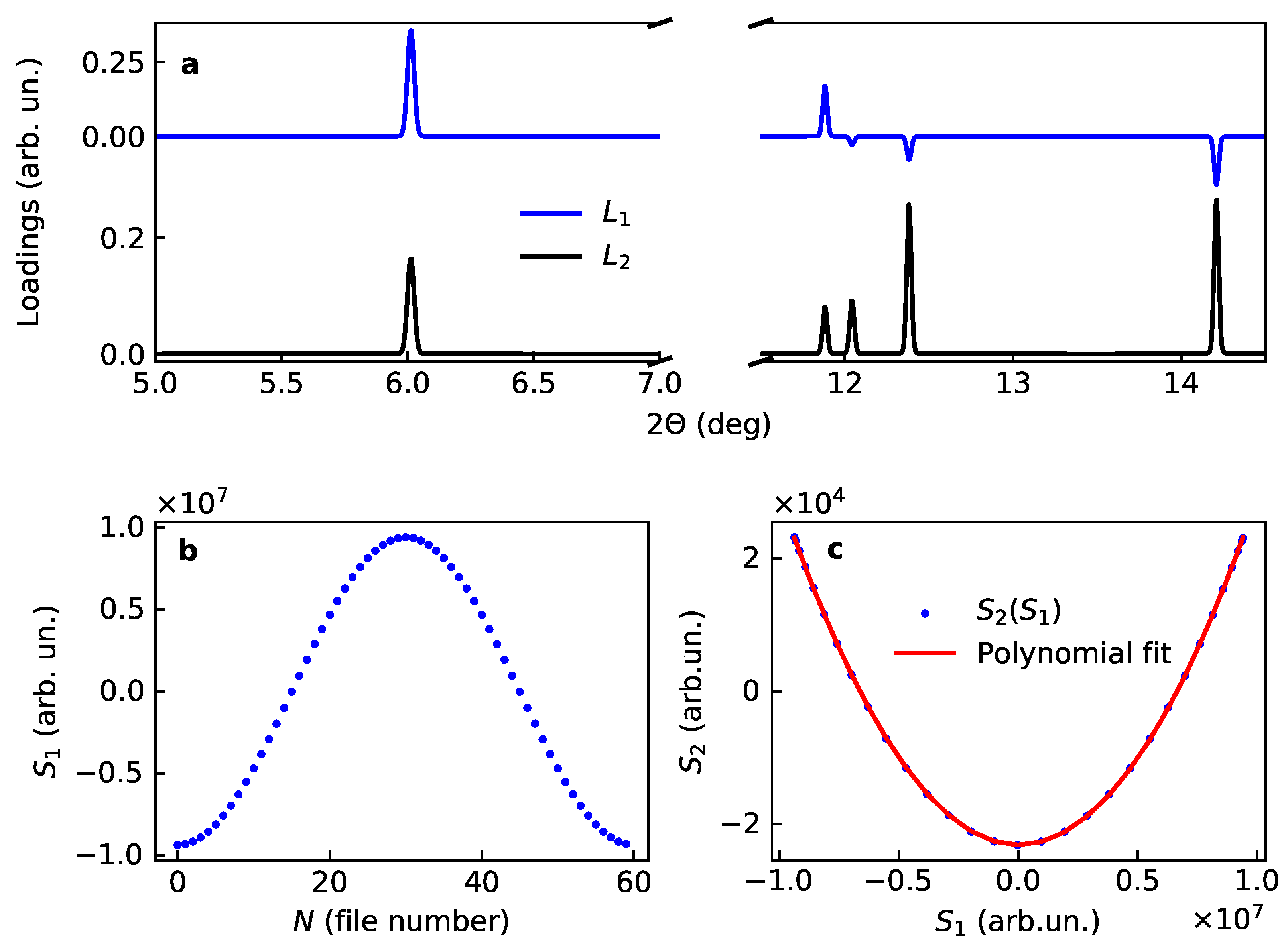
This result is in full agreement with the previously reported findings. Moreover, as it is shown in Figure 1, the first loading closely maps the cross term:
in accordance with Table 1. This case implies that both loadings are line patterns with a symmetric lineshape. The second loading consists from positive peaks of the active (varying) sublattice. The first loading is a sum of positive and negative peaks; their sign corresponds to sign of the product of structural amplitudes for the average structure and active substructure, i.e., it carries certain phase information (Figure 1).
3.1.2. Variation of Lattice Dimension
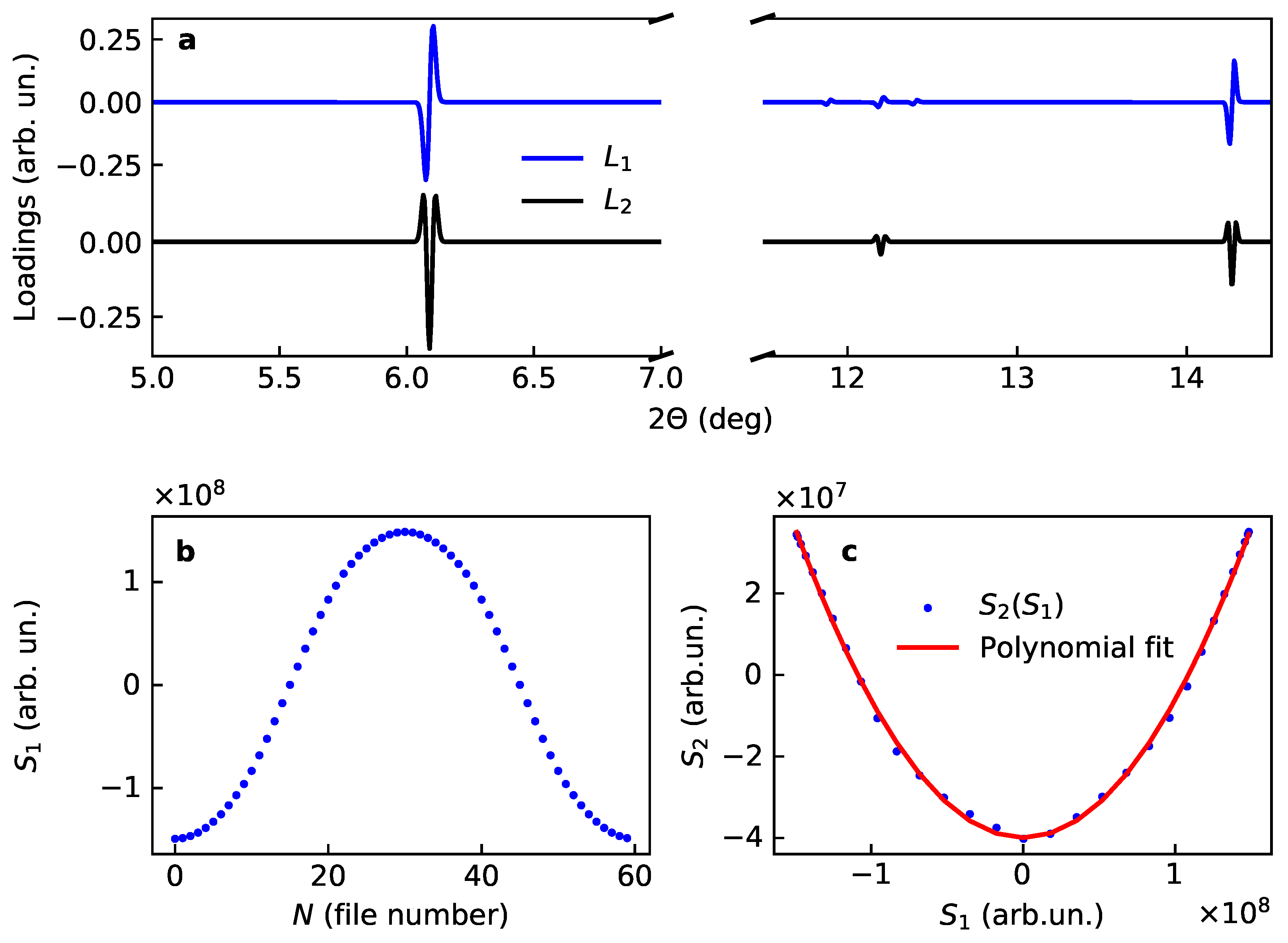
The case when only the line positions, , are changed has not been analyzed yet. According to Table 1 the following components are expected:
The analysis of the simulated data (Figure 2) agrees with what is expected from the Equation (13), namely:
- The first score is given by time dependence of the unit cell dimension;
- The second score is the square of the first score;
- The first loading is a diffractogram where every line is a first derivative of the profile function, for the considered symmetric profile of the initial data it implies an anti-symmetric line shape given by the first derivative;
- The second loading is a sum of lines whose shape is given by the second derivative of the initial profile, for the considered symmetric profile of the initial data it implies a symmetric line shape given by the second derivative.
Note, that according to Equation (13) the value and sign of the change of the line positions is encoded in the intensities of the loadings, while the positions of the intensities are given by the averaged values of the corresponding interplanar distances. Even with a limited number of terms taken into account with the Taylor expansion, the results of the PCA decomposition closely correspond to the expectations.
3.1.3. Variation of Lattice Dimension and Occupancy
When both the occupancy of Li position and the unit cell dimension c vary with time, it is natural to assume that their evolution functions are linearly related
The corresponding powder diffraction patterns are given by the following expression:
One therefore might expect that the PCA decomposition gives two scores, and , and two loadings, that may be differentiated by their profile functions. For the case when experimental information for the modelling is taken from [20], we found that the contributions from the unit cell variation largely dominate and the results are very similar to those derived for the cell variation only.
3.2. Kr Uptake by –Mg(BH)
Variation of Occupancy
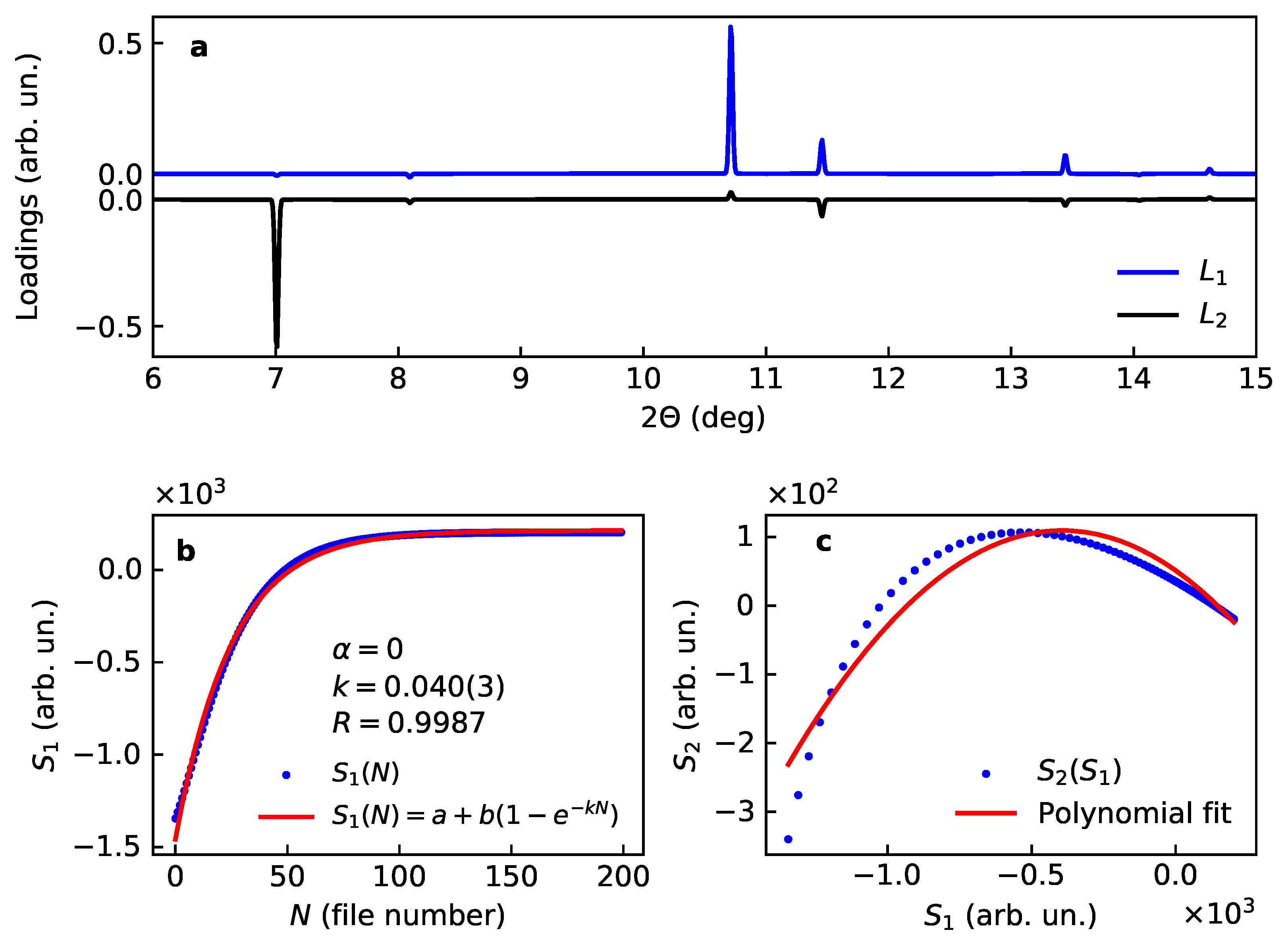
Here we return back to the case when only one occupancy is varied, and any change of the unit cell dimension or atomic coordinates are not entered in the simulation. For Kr uptake we have assumed that Kr occupancy is changing with the file number (playing the role of time) as
This case is taken as an example of the rotational ambiguity considered in the theory section. Indeed, the expectation is to see the output of PCA similar to Section 3.1.1; however, the result happens to be different, both in terms of loadings and scores (Figure 3).
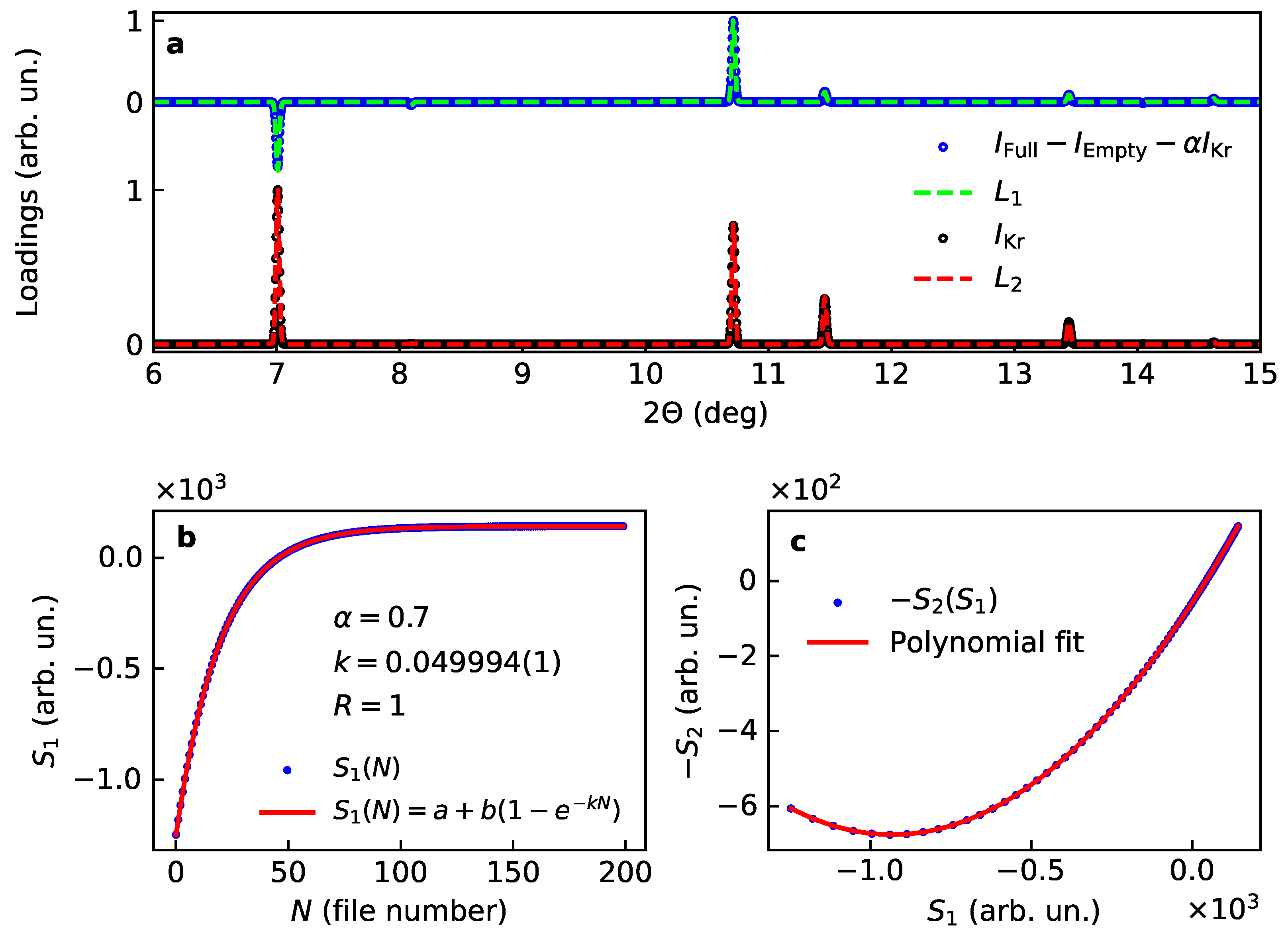
We therefore made a search for a rotational angle that provides the loadings and scores satisfying the following conditions:
- may consist both positive and negative peaks, while might be positive.
- might be proportional to the square of .
The result is shown on Figure 4 for the angle rad. There is a significant improvement of the scores, gives the same rate as the one used to calculate the data, and there is a perfect fit with a parabola for as a function of , however with a noticeable linear term. This linear term indicates that a fraction of the first component might be admixed with the second. The second loading nicely corresponds to the diffraction pattern calculated with only the Kr atoms. The first loading is essentially the cross term from Table 1. The cross term can be calculated based on structural information as follows. First, one calculates the diffraction patterns for the empty framework without Kr () and for Kr substructure without framework (). Since the diffraction intensity for the structure loaded with Kr reads
The cross-term can therefore be calculated by subtracting and from the pattern for the structure filled with Kr. In order to account for the linear term in the score correlation we had to introduce one adjustable mixing parameter a (see Figure 4a).
Therefore, all the scores and loadings receive a rational explanation and can be used to get information on the kinetics of Kr uptake from , on the structure of active Kr sublattice from , and even the crystallographic phase information stored in . However, two additional variables had to be introduced to come to this result: a rotation angle and a mixing parameter. Note, that for the considered case of single phase powder diffraction, the second score does not carry any unique information. By the very nature of diffraction phenomena the second score is proportional to the square of the first score and therefore serves for optimising the rotational correction. This exercise shows that, in spite of the rotational ambiguity, the physically meaningful components may be recovered from the PCA output provided the output is further refined with additional constraints.
4. PCA Analysis of Real Data for Mg(Bh) + Kr
The data we use for PCA are the same as used in [21]. A sequential Rietveld refinement of the data made a detailed analysis of kinetics barriers for Kr uptake by this porous solid possible [21]. A specific feature of these data is a time-dependent background that comes from Kr fluorescence. This background serves as an independent measure of the absorbed Kr and can be directly compared with the outputs of PCA.
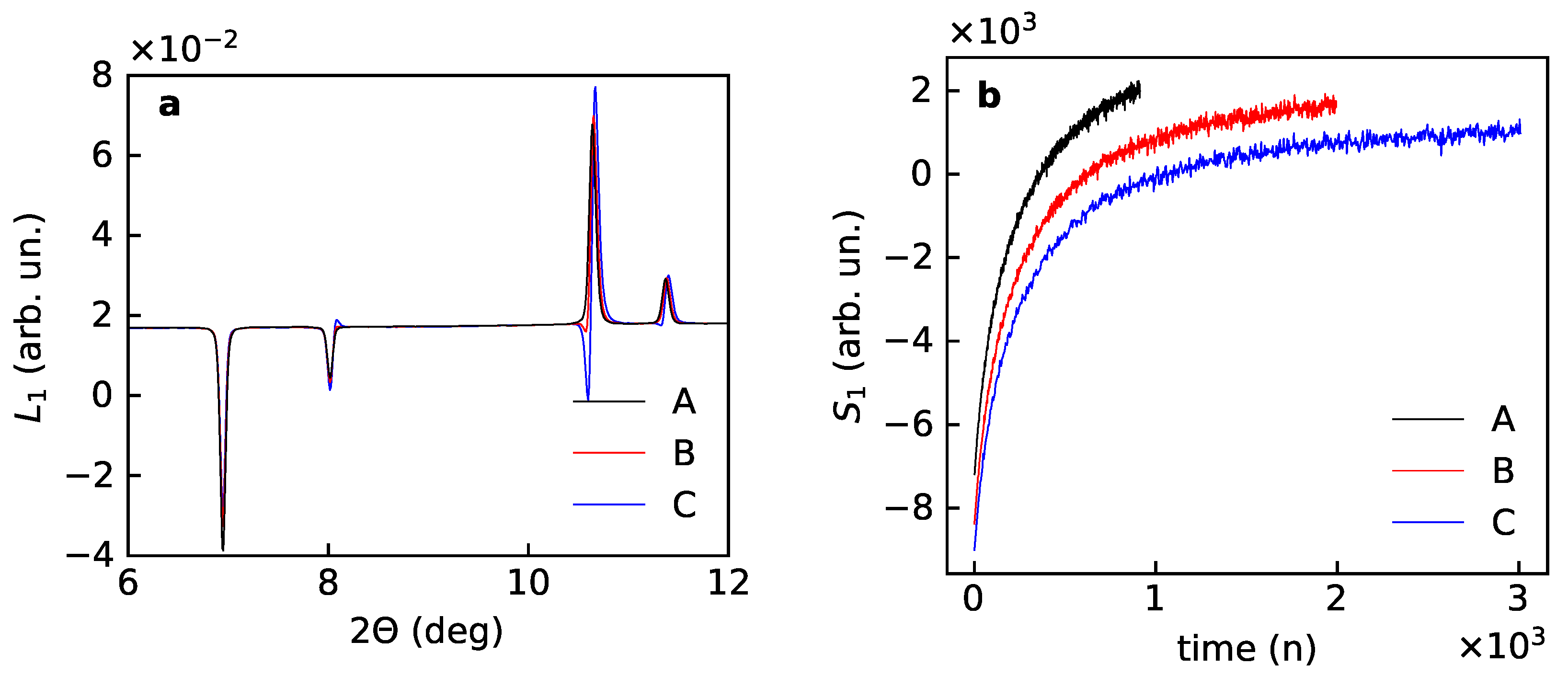
We use a dataset collected at 170 K with bar pressure of Kr, as a function of time after the “sample + gas” container was quickly inserted in the cold N stream. The data were recorded with 4 seconds time sampling. In agreement with kinetics analysis given in Ref. [21] we consider every pattern as a snapshot of the equilibrium state, an overview of this collection of powder patterns is given at Figure 5. The data were partitioned in three partial subsets, we took only first 1000 patterns of full data (subset A), than 1000 patterns with every second pattern (subset B), and finally 1000 patterns with every fourth pattern (subset C). We use this partitioning to examine how the PCA outputs from partial data correspond to each other and to the Kr fluorescence background.
The “blind” application of PCA gives results that are far from satisfactory, shown in Figure 6. The first scores can be overlapped with a constant shift with small but notable difference with the Kr background signal. The first loadings do not look the same for three subsets.
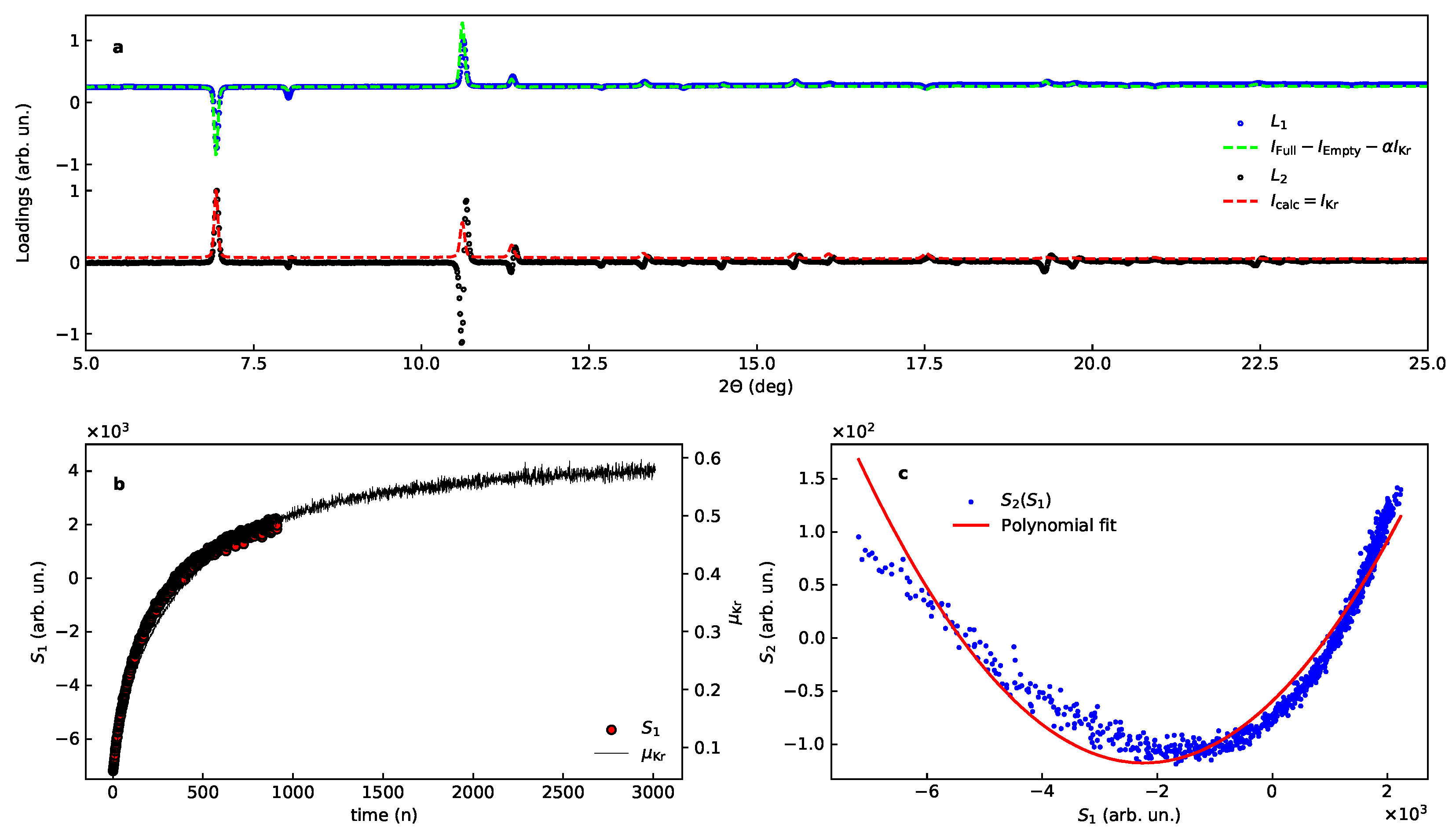
The PCA with the dataset A gives one dominating component that accounts for 99 percent of all changes, with loading and score shown in Figure 7 after a small manual rotational correction of rad. The expected evolution function and intensity distribution are given in Table 1 and in Equation (14). The comparison with intensity estimates are given for the loadings in Figure 7.
The match of the calculated loading with observed is satisfactory for , assuming one leading term (Equation (14), Table 1), namely:
similar to the model case considered above. For many lines have anti-symmetric line shapes indicating that the major contributions come from the following terms:
A comparison of the first contribution with the second loading is given in Figure 7 for the dataset A.
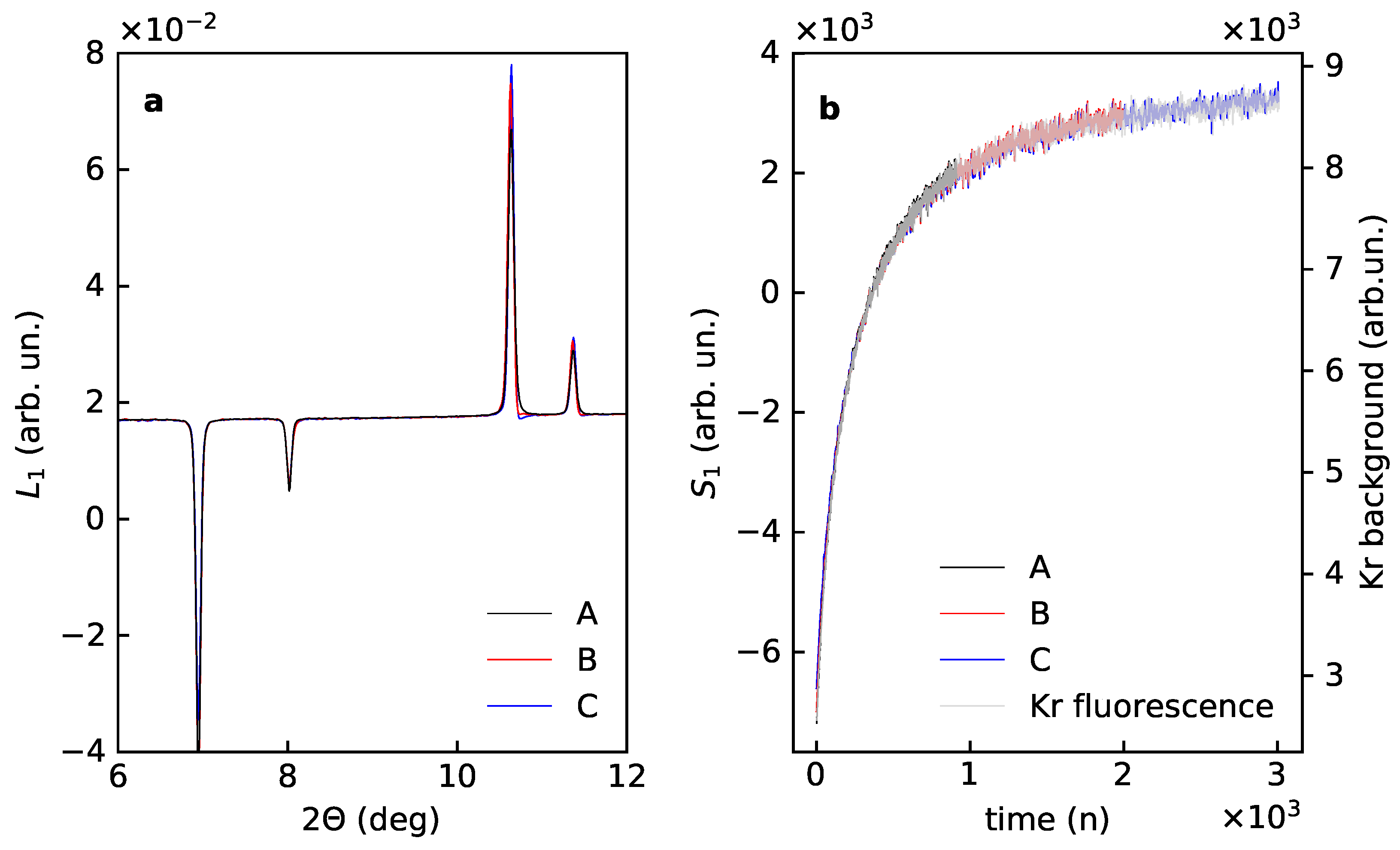
The PCA output for data subsets B and C correlates well with the results for the subset A after the rotational correction (Appendix B). After shifting with a constant all the first scores overlap and match the time dependence of the Kr fluorescence background (Figure 8). All first loadings are also looking similar, close inspection evidence a systematic shift in line positions and distortion of the shape. The shift reflects a change in the average unit cell dimension with time. The change in line shape indicates that for datasets covering longer experimental time higher order terms from Table 1 become significant. A similar effect is reflected in the second loadings, where one sees that the first term in Equation (18) goes down and the second term increases for datasets with longer time. This change in ratio of different diffraction contributions into the PCA components indicates a certain difference in time evolution for Kr occupancy and unit cell dimension: the unit cell size keeps changing when Kr occupancy is nearly saturated.
5. Conclusions
We have performed a theoretical analysis on how specific changes in time resolved diffraction data are represented into PCA output. The analysis enumerates terms that comes alone or as linear combinations into loadings and scores given by PCA. The above analysis is illustrated by applications of PCA to synthetic and real powder diffraction data. The immediate result shows that this method has an inherent danger when it is applied “blindly”, that is sometimes considered as an advantage. Namely loadings may have a complex structure being a sum of contributions mixing up the lattice and structural response. Leaving quantitative analysis of the loadings aside and focusing on solely on the, e.g., kinetic information extracted from the scores is not less dangerous. Rotational ambiguity makes certain linear combinations of diffraction contributions to be preferred components for PCA, resulting in inaccurate rates and activation energies when applied blindly. The first practical recommendation stemming from the theoretical analysis is to find a rotation correction that makes as close as possible to a square of . Successful applications of this recommendation were exemplified with both simulated and real data. We have also shown that the loadings can be rationalized in terms of contributions with different profile functions. The decomposition on contributions is trivial for powder diffraction if there is no change in the unit cell dimension. This makes PCA an interesting tool for single crystal applications where diffraction intensities can be collected independently from unit cell changes [19]. The information stored in loadings may be used to analyse active (responsive, evolving) substructure from the second loading, or to retrieve partial phase information from the first loading that is defined by the cross-product of structure factors. For powder diffraction additional information is contained in the line shapes. Thus, for an optimal rotational correction the line shapes of low angle reflections for first loading are predominantly symmetric functions of Bragg angle, while for the second loading that may be a sum of both, symmetric and anti-symmetric profiles.
The number of applications of PCA for the fast analysis of big diffraction data will certainly grow. It is one of the efficient data tools that are highly requested especially for very productive large scale experimental facilities. However, a successful use of PCA necessarily implies that the results are carefully analyzed and a further manual rotational correction is applied. If the PCA output is used blindly, the outputs have to be taken with a grain of salt, as we have shown here they almost certainly contain no physically meaningful result.
The other possible option is to use Multivariate curve resolution with alternating least squares (MCR–ALS), see Ref. [8] as an example. This method, being based on PCA, allows one to constrain the output. For a diffraction probe of structural processes, the constraints have to be set accounting for the diffraction components listed in Table 1. Potentially MCR–ALS, as well as post-PCA corrections, like OCCR [17], with proper constraints may be used for targeting individual diffraction contributions. The possible constrains might be based on the shape of corresponding profile functions, but their exact formulation and quantitative analysis need more theoretical efforts and model calculations.
In spite of the difficulties and complications listed above, the interpretation of the PCA applied to single phase powder diffraction is entirely possible with all contributions enumerated in Table 1. The present report provides one more step towards the rational use of PCA and similar multivariate tools to diffraction data. The next steps in the development and understanding may include quantitative analysis of the loadings, and development of the software tools for on-line analysis of data from in situ experiments.
Author Contributions
Conceptualization, D.C.; methodology, D.C.; software, V.D.; validation, W.v.B.; formal analysis, D.C.; data curation I.D., V.D. and W.v.B.; writing–original draft preparation, D.C. and V.D.; visualization, V.D.; supervision, W.v.B.; project administration, W.v.B. All authors have read and agreed to the published version of the manuscript.
Funding
This research received no external funding.
Conflicts of Interest
The authors declare no conflict of interest.
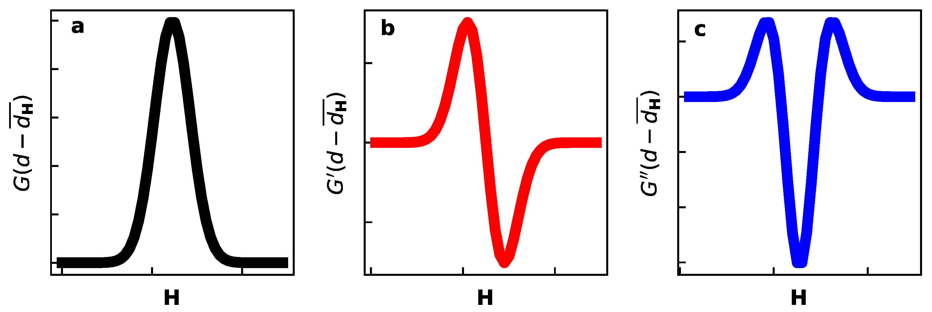
Appendix A
The profile functions for diffraction components listed in Table 1 are given by corresponding derivatives of the initial profile. Initial line shape is defined, as usual, by a convolution of the resolution function of diffractometer and the scattering function of sample. Here we take as an example a Gaussian profile,
The derivatives are
The graphical representation of the above profile functions are shown in Figure A1.
Figure A1.
Profile functions for diffraction components from Table 1: (a), (b), and (c).
Figure A1.
Profile functions for diffraction components from Table 1: (a), (b), and (c).

The loadings given by PCA are sums of contributions with these profiles, and can therefore be decomposed into components for a subsequent structural analysis.
The major contributions mapping component with the same evolution function (Table 1) are:
Therefore, the corresponding pattern has predominantly symmetric line shape G at small , there is an increase of the second anti-symmetric term with . The same trend is generally expected for the second pattern , the details depend of the susceptibilities and .
If the only varied parameter is occupancy of a single crystallographic site, then the structural susceptibility is simply a structural factor for the given sub-lattice.
This susceptibility becomes more complex and anisotropic if we assume that occupancy variation is associated with the change of atomic position, for example like with . For this case the susceptibility reads
Lattice susceptibility for a cubic structure with varied unit cell dimension a is simply
This susceptibility increases with Bragg angle and therefore the anti-symmetric terms in Equation (A3) are more pronounced at the high angles.
Appendix B
The rotational correction Equation (10) implies the following transformations Equation (9):
where and denote loadings and scores of the PCA output, and are loadings and scores after rotational correction with parameter . In preset work the parameter has been optimised by hand with the following criteria:
- as a function of fits with second order polynomial with best R-factor
- gives a pattern of positive or negative symmetric peaks at least at low-angle part of the pattern.
- and for different data subsets are as close to each other as possible.
The values of rotation parameter used for calculations plotted in Figure 8, are summarized in Table A1.

Table A1.
Rotation correction parameter used for Mg(BH)Kr datasets.
| Subset | |
|---|---|
| A | 0.02 |
| B | 0.095 |
| C | 0.14 |
References
- Guccione, P.; Palin, L.; Belviso, B.D.; Milanesio, M.; Caliandro, R. Principal component analysis for automatic extraction of solid-state kinetics from combined in situ experiments. Phys. Chem. Chem. Phys. PCCP 2018, 20, 19560–19571. [Google Scholar] [CrossRef] [PubMed]
- Massart, D.; Vandeginste, B.; Buydens, L.; De Jong, S.; Lewi, P.; Smeyers-Verbeke, J. Chapter 17 Principal components. In Handbook of Chemometrics and Qualimetrics: Part A; Data Handling in Science and Technology; Elsevier: Amsterdam, The Netherlands, 1998; Volume 20, pp. 519–556. [Google Scholar] [CrossRef]
- Abdi, H.; Williams, L.J. Principal component analysis. WIREs Comput. Stat. 2010, 2, 433–459. [Google Scholar] [CrossRef]
- Mitsui, T.; Okuyama, S.; Fujimura, Y. Determination of the Blend Composition Ratio of Cocaine to Sodium Hydrogencarbonate by X-Ray Diffraction Using Multivariate Analysis. Anal. Sci. 1991, 7, 941–945. [Google Scholar] [CrossRef] [Green Version]
- Hida, M.; Sato, H.; Sugawara, H.; Mitsui, T. Classification of counterfeit coins using multivariate analysis with X-ray diffraction and X-ray fluorescence methods. Forensic Sci. Int. 2001, 115, 129–134. [Google Scholar] [CrossRef]
- Jette, O.; Kurt, N.; Kenny, S. Using X-ray powder diffraction and principal component analysis to determine structural properties for bulk samples of multiwall carbon nanotubes. Z. Kristallogr. 2007, 222, 186. [Google Scholar] [CrossRef]
- O’Flynn, D.; Reid, C.B.; Christodoulou, C.; Wilson, M.D.; Veale, M.C.; Seller, P.; Hills, D.; Desai, H.; Wong, B.; Speller, R. Explosive detection using pixellated X-ray diffraction (PixD). J. Instrum. 2013, 8, P03007. [Google Scholar] [CrossRef]
- Rodriguez, M.A.; Keenan, M.R.; Nagasubramanian, G. in situ X-ray diffraction analysis of (CFx)n batteries: Signal extraction by multivariate analysis. J. Appl. Crystallogr. 2007, 40, 1097–1104. [Google Scholar] [CrossRef]
- Norrman, M.; Ståhl, K.; Schluckebier, G.; Al-Karadaghi, S. Characterization of insulin microcrystals using powder diffraction and multivariate data analysis. J. Appl. Crystallogr. 2006, 39, 391–400. [Google Scholar] [CrossRef] [Green Version]
- Caliandro, R.; Altamura, D.; Belviso, B.D.; Rizzo, A.; Masi, S.; Giannini, C. Investigating temperature-induced structural changes of lead halide perovskites by in situ X-ray powder diffraction. J. Appl. Crystallogr. 2019, 52, 1104–1118. [Google Scholar] [CrossRef]
- Chernyshov, D.; van Beek, W.; Emerich, H.; Milanesio, M.; Urakawa, A.; Viterbo, D.; Palin, L.; Caliandro, R. Kinematic diffraction on a structure with periodically varying scattering function. Acta Crystallogr. Sect. A 2011, 67, 327–335. [Google Scholar] [CrossRef] [PubMed]
- Caliandro, R.; Chernyshov, D.; Emerich, H.; Milanesio, M.; Palin, L.; Urakawa, A.; Van Beek, W.; Viterbo, D. Patterson selectivity by modulation-enhanced diffraction. J. Appl. Crystallogr. 2012, 45, 458–470. [Google Scholar] [CrossRef]
- Van Beek, W.; Emerich, H.; Urakawa, A.; Palin, L.; Milanesio, M.; Caliandro, R.; Viterbo, D.; Chernyshov, D. Untangling diffraction intensity: Modulation enhanced diffraction on ZrO2 powder. J. Appl. Crystallogr. 2012, 45, 738–747. [Google Scholar] [CrossRef]
- Chernyshov, D.; Dyadkin, V.; Van Beek, W.; Urakawa, A. Frequency analysis for modulation-enhanced powder diffraction. Acta Crystallogr. Sect. A 2016, 72, 500–506. [Google Scholar] [CrossRef] [PubMed]
- Palin, L.; Caliandro, R.; Viterbo, D.; Milanesio, M. Chemical selectivity in structure determination by the time dependent analysis of in situ XRPD data: A clear view of Xe thermal behavior inside a MFI zeolite. Phys. Chem. Chem. Phys. 2015, 17, 17480–17493. [Google Scholar] [CrossRef] [PubMed]
- Harman, H. Modern Factor Analysis, 3rd ed.; The University of Chicago Press: Chicago, IL, USA, 1976. [Google Scholar]
- Caliandro, R.; Guccione, P.; Nico, G.; Tutuncu, G.; Hanson, J.C. Tailored multivariate analysis for modulated enhanced diffraction. J. Appl. Crystallogr. 2015, 48, 1679–1691. [Google Scholar] [CrossRef]
- Guccione, P.; Palin, L.; Milanesio, M.; Belviso, B.D.; Caliandro, R. Improved multivariate analysis for fast and selective monitoring of structural dynamics by in situ X-ray powder diffraction. Phys. Chem. Chem. Phys. 2018, 20, 2175–2187. [Google Scholar] [CrossRef] [PubMed]
- Conterosito, E.; Palin, L.; Caliandro, R.; van Beek, W.; Chernyshov, D.; Milanesio, M. CO2 adsorption in Y zeolite: A structural and dynamic view by a novel principal-component-analysis-assisted in situ single-crystal X-ray diffraction experiment. Acta Crystallogr. Sect. A 2019, 75, 214–222. [Google Scholar] [CrossRef] [PubMed]
- Laubach, S.; Laubach, S.; Schmidt, P.C.; Ensling, D.; Schmid, S.; Jaegermann, W.; Thißen, A.; Nikolowski, K.; Ehrenberg, H. Changes in the crystal and electronic structure of LiCoO2 and LiNiO2 upon Li intercalation and de-intercalation. Phys. Chem. Chem. Phys. 2009, 11, 3278–3289. [Google Scholar] [CrossRef] [PubMed]
- Dovgaliuk, I.; Senkovska, I.; Xiao, L.; Dyadkin, V.; Filinchuk, Y.; Chernyshov, D. Kinetic Barriers and Microscopic Mechanism of Gas Adsorption by Sub-Second X-Ray Diffraction: Case for Kr in Nanoporous γ-Mg(BH4)2. Angew. Chem. 2020. Submitted. [Google Scholar]
- Caliandro, R.; Belviso, D.B. RootProf: Software for multivariate analysis of unidimensional profiles. J. Appl. Crystallogr. 2014, 47, 1087–1096. [Google Scholar] [CrossRef]
Figure 1.
Loadings and scores for two main components for the model case of variation of the occupancy in LiCoO: (a) loadings and , (b) first score and (c) correlation plot for the scores, together with the polinomial fit.
Figure 1.
Loadings and scores for two main components for the model case of variation of the occupancy in LiCoO: (a) loadings and , (b) first score and (c) correlation plot for the scores, together with the polinomial fit.

Figure 2.
Loadings and scores for two main components for the model case of variation of lattice dimension in LiCoO: (a) loadings and , (b) first score and (c) correlation plot for the scores, together with the polinomial fit.
Figure 2.
Loadings and scores for two main components for the model case of variation of lattice dimension in LiCoO: (a) loadings and , (b) first score and (c) correlation plot for the scores, together with the polinomial fit.

Figure 3.
Loadings (a) and scores (b,c) for two main components for the model case of Kr uptake by the porous –Mg(BH). (b) shows the first score with the fit for the expected kinetics, note the difference between the refined rate () and the model value (). (c) shows the correlation between the scores and where the line stays for the best fit of a second-order polynomial function.

Figure 4.
Loadings (a) and scores (b,c) for two main components for the model case of Kr uptake by the porous –Mg(BH) after rotation corrections. The first score is shown togther with a fit (b), note the perfect agreement between the fitted and the model rates (). The correlation between scores and together with the best fit with a second-order polynomial function is shown in (c).

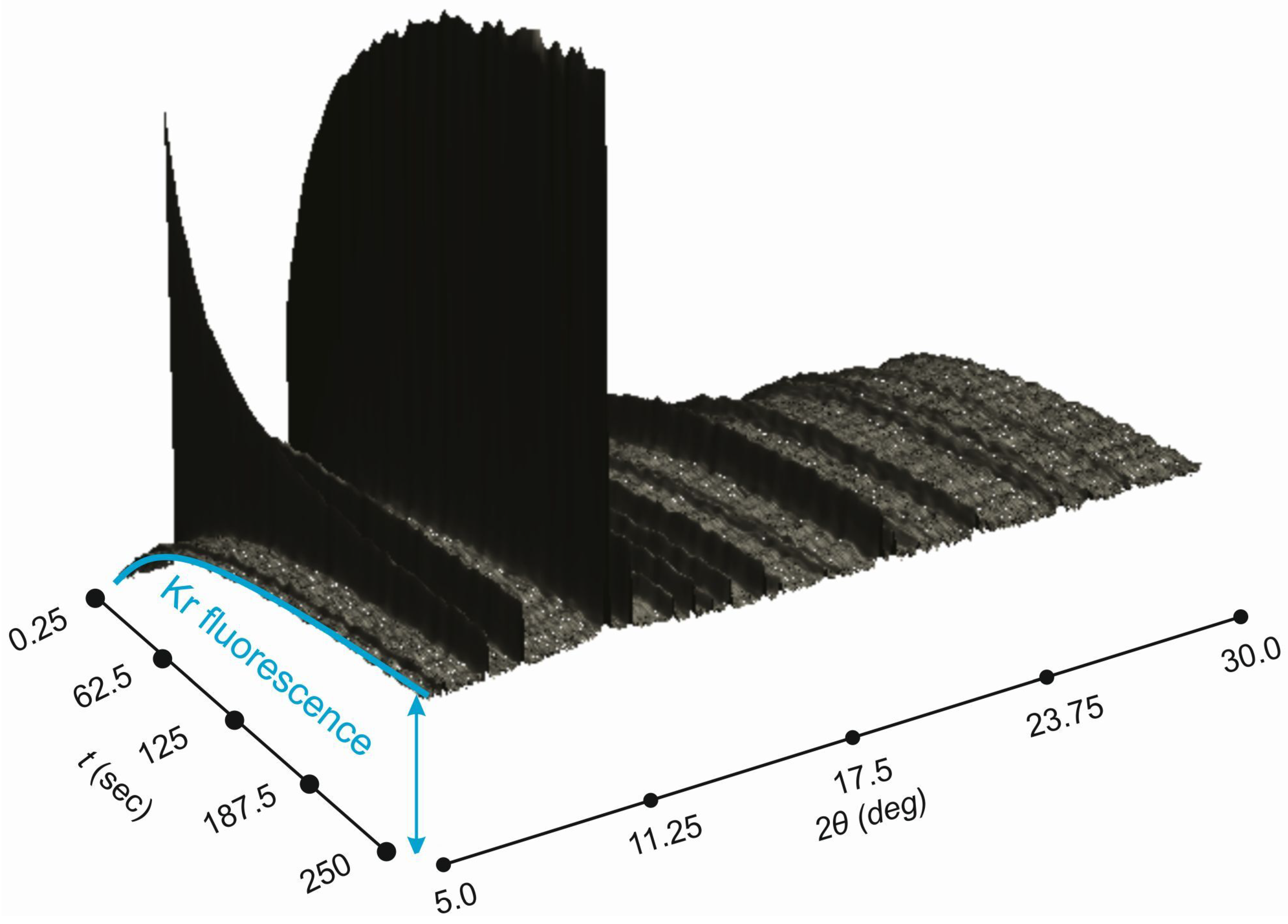
Figure 5.
Powder diffraction data collected as a function of time during Kr uptake by –Mg(BH) at 170 K. Note Kr fluorescence background that gives additional measure of Kr in the irradiated volume.
Figure 5.
Powder diffraction data collected as a function of time during Kr uptake by –Mg(BH) at 170 K. Note Kr fluorescence background that gives additional measure of Kr in the irradiated volume.

Figure 6.
First loadings (a) and scores (b) after PCA for the experimental data for Kr uptake by the porous magnesium borohydrate –Mg(BH) for subsets A (first 1000 powder patterns), B (1000 patterns with every second pattern), C (1000 patterns with every fourth pattern).
Figure 6.
First loadings (a) and scores (b) after PCA for the experimental data for Kr uptake by the porous magnesium borohydrate –Mg(BH) for subsets A (first 1000 powder patterns), B (1000 patterns with every second pattern), C (1000 patterns with every fourth pattern).

Figure 7.
PCA of the experimental data, subset A, for Kr uptake by –Mg(BH) after the rotational correction (see text). (a) Loadings, corrected for the rotation, bottom shows and overlay of the second loading (black circles) together with the diffraction pattern from the Kr sublattice alone (red line). (b) shows the first score with together with Kr occupancy. (c) shows the correlation between the scores with line for a best fit with a second order polynomial function.

Figure 8.
First loadings (a) and scores (b) corrected for the rotation for the experimental data for Kr uptake by the porous magnesium borohydrate –Mg(BH) for the subsets A (first 1000 powder patterns), B (1000 patterns with every second pattern), C (1000 patterns with every fourth pattern).
Figure 8.
First loadings (a) and scores (b) corrected for the rotation for the experimental data for Kr uptake by the porous magnesium borohydrate –Mg(BH) for the subsets A (first 1000 powder patterns), B (1000 patterns with every second pattern), C (1000 patterns with every fourth pattern).

Table 1.
Time evolution functions and intensity distributions for components in Equation (7).
Table 1.
Time evolution functions and intensity distributions for components in Equation (7).
| n | ||
|---|---|---|
| 1 | ||
| 2 | ||
| 3 | ||
| 4 | ||
| 5 | ||
| 6 | ||
| 7 | 2 | |
| 8 |
© 2020 by the authors. Licensee MDPI, Basel, Switzerland. This article is an open access article distributed under the terms and conditions of the Creative Commons Attribution (CC BY) license (http://creativecommons.org/licenses/by/4.0/).
Share and Cite
MDPI and ACS Style
Chernyshov, D.; Dovgaliuk, I.; Dyadkin, V.; van Beek, W. Principal Component Analysis (PCA) for Powder Diffraction Data: Towards Unblinded Applications. Crystals 2020, 10, 581. https://0-doi-org.brum.beds.ac.uk/10.3390/cryst10070581
AMA Style
Chernyshov D, Dovgaliuk I, Dyadkin V, van Beek W. Principal Component Analysis (PCA) for Powder Diffraction Data: Towards Unblinded Applications. Crystals. 2020; 10(7):581. https://0-doi-org.brum.beds.ac.uk/10.3390/cryst10070581
Chicago/Turabian StyleChernyshov, Dmitry, Iurii Dovgaliuk, Vadim Dyadkin, and Wouter van Beek. 2020. "Principal Component Analysis (PCA) for Powder Diffraction Data: Towards Unblinded Applications" Crystals 10, no. 7: 581. https://0-doi-org.brum.beds.ac.uk/10.3390/cryst10070581
Note that from the first issue of 2016, this journal uses article numbers instead of page numbers. See further details here.